x ray methods

9.1

SECTION 9X-RAY METHODS

9.1 PRODUCTION OF X-RAYS AND X-RAY SPECTRA 9.2

9.2 INSTRUMENTATION 9.3

9.2.1 X-Ray Tubes 9.3

Table 9.1 Wavelengths of X-Ray Emission Spectra in Angstroms 9.4

Table 9.2 Wavelengths (in Angstroms) of Absorption Edges 9.6

Table 9.3 Critical X-Ray Absorption Energies in keV 9.8

Table 9.4 X-Ray Emission Energies in keV 9.10

Figure 9.1 Geometry of a Plane-Crystal X-Ray Fluorescence Spectrometer 9.12

9.2.2 Collimators and Filters 9.12

9.2.3 Analyzing Crystals 9.12

Table 9.5 � Filters for Common Target Elements 9.13

Table 9.6 Analyzing Crystals for X-Ray Spectroscopy 9.13

9.3 DETECTORS 9.14

9.3.1 Proportional Counters 9.14

9.3.2 Scintillation Counters 9.14

9.3.3 Lithium-Drifted Semiconductor Detectors 9.14

9.3.4 Comparison of X-Ray Detectors 9.15

9.4 PULSE-HEIGHT DISCRIMINATION 9.15

9.5 X-RAY ABSORPTION METHODS 9.15

9.5.1 Principle 9.15

9.5.2 Radiography 9.16

9.6 X-RAY FLUORESCENCE METHOD 9.16


Table 9.7 Mass Absorption Coefficients for K�1

Lines and W L�1

Line 9.17

9.6.2 Instrumentation 9.19

9.6.3 Sample Handling 9.19

9.6.4 Matrix Effects 9.19

9.7 ENERGY-DISPERSIVE X-RAY SPECTROMETRY 9.20

9.8 ELECTRON-PROBE MICROANALYSIS 9.20

9.9 ELECTRON SPECTROSCOPY FOR CHEMICAL APPLICATIONS (ESCA) 9.20


9.9.2 Chemical Shifts 9.21

9.9.3 ESCA Instrumentation 9.21

9.9.4 Uses 9.21

9.10 AUGER EMISSION SPECTROSCOPY (AES) 9.21

9.11 X-RAY DIFFRACTION 9.22


Table 9.8 Interplanar Spacings for K�1

Radiation, d versus 2� 9.23

9.11.2 Powder Diffraction 9.24

9.11.3 Polymer Characterization 9.24

9.11.4 Single-Crystal Structure Determination 9.25

Bibliography 9.25

Downloaded from Digital Engineering Library @ McGraw-Hill (www.digitalengineeringlibrary.com)Copyright © 2004 The McGraw-Hill Companies. All rights reserved.

Any use is subject to the Terms of Use as given at the website.

Source: DEAN’S ANALYTICAL CHEMISTRY HANDBOOK

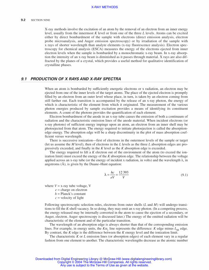
X-ray methods involve the excitation of an atom by the removal of an electron from an inner energylevel, usually from the innermost K level or from one of the three L levels. Atoms can be excitedeither by direct bombardment of the sample with electrons (direct emission analysis, electronprobe microanalysis, and Auger emission spectroscopy) or by irradiation of the sample with x rays of shorter wavelength than analyte elements (x-ray fluorescence analysis). Electron spec-troscopy for chemical analysis (ESCA) measures the energy of the electrons ejected from innerelectron levels when the sample is bombarded by a monochromatic x-ray beam. In x-ray absorp-tion the intensity of an x-ray beam is diminished as it passes through material. X rays are also dif-fracted by the planes of a crystal, which provides a useful method for qualitative identification ofcrystalline phases.

9.1 PRODUCTION OF X RAYS AND X-RAY SPECTRA

When an atom is bombarded by sufficiently energetic electrons or x radiation, an electron may beejected from one of the inner levels of the target atoms. The place of the ejected electron is promptlyfilled by an electron from an outer level whose place, in turn, is taken by an electron coming fromstill farther out. Each transition is accompanied by the release of an x-ray photon, the energy ofwhich is characteristic of the element from which it originated. The measurement of the variousphoton energies produced by sample excitation provides a means of identifying its constituentelements. A count of the photons provides the quantification of each element.

Electron bombardment of the anode in an x-ray tube causes the emission of both a continuum ofradiation and the characteristic emission lines of the anode material. When incident electrons (orx-ray photons) of sufficient energy impinge upon an atom, an electron from an inner shell may bephotoejected from that atom. The energy required to initiate photoejection is called the absorption-edge energy. The absorption edge will be a sharp discontinuity in the plot of mass absorption coef-ficient versus wavelength.

There is successive ionization—first of electrons in the outermost levels of the sample or target(let us assume the M level), then of electrons in the L levels as the three L absorption edges are pro-gressively exceeded, and finally in the K level as the K absorption edge is exceeded.

The energy required to lift a K electron out of the environment of the atom (to exceed the ion-ization limit) must exceed the energy of the K absorption edge. The relationship between the voltageapplied across an x-ray tube (or the energy of incident x radiation, in volts) and the wavelength λ, inangstroms (Å), is given by the Duane–Hunt equation:

(9.1)

where V = x-ray tube voltage, Ve = charge on electronh = Planck’s constantc = velocity of light

Following spectroscopic selection rules, electrons from outer shells (L and M) will undergo transi-tions to fill the K-shell vacancy. In so doing, they may emit an x-ray photon. (In a competing process,the energy released may be internally converted in the atom to cause the ejection of a secondary, orAuger, electron. Auger spectroscopy is discussed later.) The energy of the emitted radiation will becharacteristic of the element and of the particular transition.

The wavelength of an absorption edge is always shorter than that of the corresponding emissionlines. For example, in energy units, the Ka1 line represents the difference: K edge minus LIII edge.By contrast, the K edge is the difference between the K energy level and the ionization limit.

The characteristic K or L emission lines (or absorption edges) of each element vary in a regularfashion from one element to another. The characteristic wavelengths decrease as the atomic number

λ = =hc

eV V

12 393

9.2 SECTION NINE



X-RAY METHODS

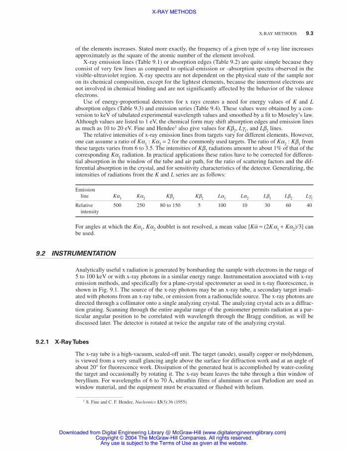
of the elements increases. Stated more exactly, the frequency of a given type of x-ray line increasesapproximately as the square of the atomic number of the element involved.

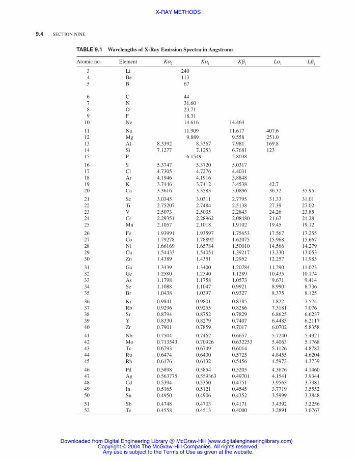
X-ray emission lines (Table 9.1) or absorption edges (Table 9.2) are quite simple because theyconsist of very few lines as compared to optical-emission or -absorption spectra observed in thevisible-ultraviolet region. X-ray spectra are not dependent on the physical state of the sample noron its chemical composition, except for the lightest elements, because the innermost electrons arenot involved in chemical binding and are not significantly affected by the behavior of the valenceelectrons.

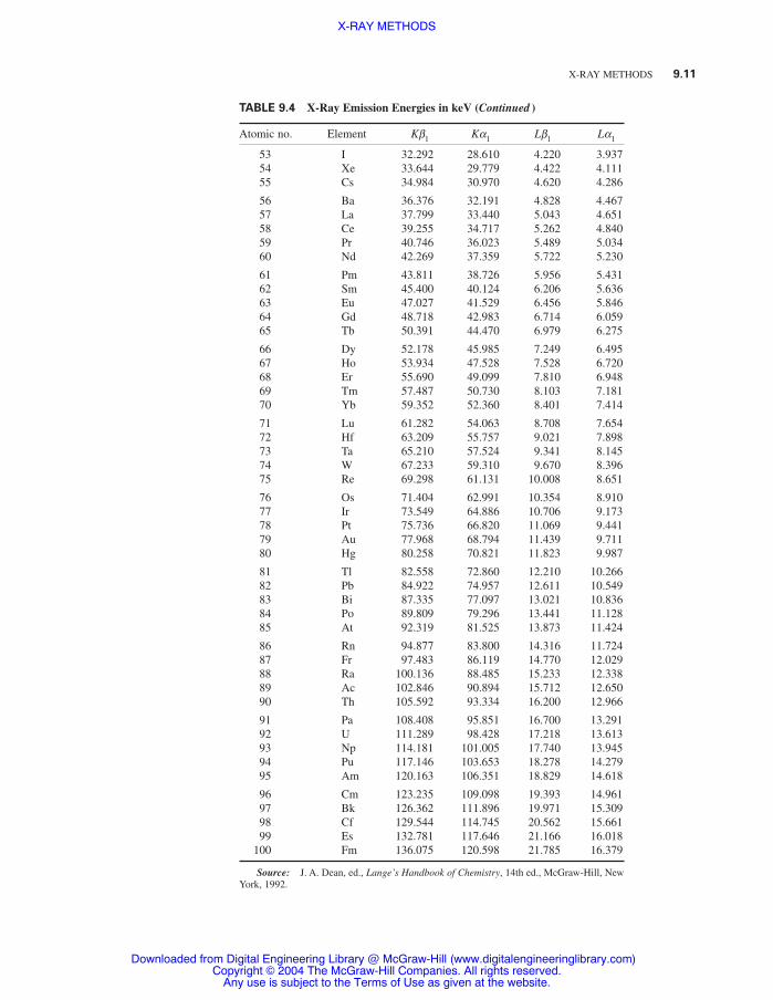
Use of energy-proportional detectors for x rays creates a need for energy values of K and Labsorption edges (Table 9.3) and emission series (Table 9.4). These values were obtained by a con-version to keV of tabulated experimental wavelength values and smoothed by a fit to Moseley’s law.Although values are listed to 1 eV, the chemical form may shift absorption edges and emission linesas much as 10 to 20 eV. Fine and Hendee1 also give values for Kb2, Lg1, and Lb2 lines.

The relative intensities of x-ray emission lines from targets vary for different elements. However,one can assume a ratio of Ka1 : Ka2 = 2 for the commonly used targets. The ratio of Ka2 : Kb1 fromthese targets varies from 6 to 3.5. The intensities of Kb2 radiations amount to about 1% of that of thecorresponding Ka1 radiation. In practical applications these ratios have to be corrected for differen-tial absorption in the window of the tube and air path, for the ratio of scattering factors and the dif-ferential absorption in the crystal, and for sensitivity characteristics of the detector. Generalizing, theintensities of radiations from the K and L series are as follows:

Emissionline Ka1 Ka2 Kb1 Kb2 La1 La2 Lb1 Lb2 Lg1

Relative 500 250 80 to 150 5 100 10 30 60 40intensity

For angles at which the Ka1, Ka2 doublet is not resolved, a mean value [K −a = (2Ka1 + Ka2)/3] canbe used.

9.2 INSTRUMENTATION

Analytically useful x radiation is generated by bombarding the sample with electrons in the range of5 to 100 keV or with x-ray photons in a similar energy range. Instrumentation associated with x-rayemission methods, and specifically for a plane-crystal spectrometer as used in x-ray fluorescence, isshown in Fig. 9.1. The source of the x-ray photons may be an x-ray tube, a secondary target irradi-ated with photons from an x-ray tube, or emission from a radionuclide source. The x-ray photons aredirected through a collimator onto a single analyzing crystal. The analyzing crystal acts as a diffrac-tion grating. Scanning through the entire angular range of the goniometer permits radiation at a par-ticular angular position to be correlated with wavelength through the Bragg condition, as will bediscussed later. The detector is rotated at twice the angular rate of the analyzing crystal.

9.2.1 X-Ray Tubes

The x-ray tube is a high-vacuum, sealed-off unit. The target (anode), usually copper or molybdenum,is viewed from a very small glancing angle above the surface for diffraction work and at an angle ofabout 20° for fluorescence work. Dissipation of the generated heat is accomplished by water-coolingthe target and occasionally by rotating it. The x-ray beam leaves the tube through a thin window ofberyllium. For wavelengths of 6 to 70 Å, ultrathin films of aluminum or cast Parlodion are used aswindow material, and the equipment must be evacuated or flushed with helium.

X-RAY METHODS 9.3

1 S. Fine and C. F. Hendee, Nucleonics 13(3):36 (1955).



X-RAY METHODS

9.4 SECTION NINE

TABLE 9.1 Wavelengths of X-Ray Emission Spectra in Angstroms

Atomic no. Element Ka2 Ka1 Kb1 La1 Lb1

3 Li 2404 Be 1135 B 67

6 C 447 N 31.608 O 23.719 F 18.31

10 Ne 14.616 14.464

11 Na 11.909 11.617 407.612 Mg 9.889 9.558 251.013 Al 8.3392 8.3367 7.981 169.814 Si 7.1277 7.1253 6.7681 12315 P 6.1549 5.8038

16 S 5.3747 5.3720 5.031717 Cl 4.7305 4.7276 4.403118 Ar 4.1946 4.1916 3.884819 K 3.7446 3.7412 3.4538 42.720 Ca 3.3616 3.3583 3.0896 36.32 35.95

21 Sc 3.0345 3.0311 2.7795 31.33 31.0122 Ti 2.75207 2.7484 2.5138 27.39 27.0223 V 2.5073 2.5035 2.2843 24.26 23.8524 Cr 2.29351 2.28962 2.08480 21.67 21.2825 Mn 2.1057 2.1018 1.9102 19.45 19.12

26 Fe 1.93991 1.93597 1.75653 17.567 17.25527 Co 1.79278 1.78892 1.62075 15.968 15.66728 Ni 1.66169 1.65784 1.50010 14.566 14.27929 Cu 1.54433 1.54051 1.39217 13.330 13.05330 Zn 1.4389 1.4351 1.2952 12.257 11.985

31 Ga 1.3439 1.3400 1.20784 11.290 11.02332 Ge 1.2580 1.2540 1.1289 10.435 10.17433 As 1.1798 1.1758 1.0573 9.671 9.41434 Se 1.1088 1.1047 0.9921 8.990 8.73635 Br 1.0438 1.0397 0.9327 8.375 8.125

36 Kr 0.9841 0.9801 0.8785 7.822 7.57437 Rb 0.9296 0.9255 0.8286 7.3181 7.07638 Sr 0.8794 0.8752 0.7829 6.8625 6.623739 Y 0.8330 0.8279 0.7407 6.4485 6.211740 Zr 0.7901 0.7859 0.7017 6.0702 5.8358

41 Nb 0.7504 0.7462 0.6657 5.7240 5.492142 Mo 0.713543 0.70926 0.632253 5.4063 5.176843 Tc 0.6793 0.6749 0.6014 5.1126 4.878244 Ru 0.6474 0.6430 0.5725 4.8455 4.620445 Rh 0.6176 0.6132 0.5456 4.5973 4.3739

46 Pd 0.5898 0.5854 0.5205 4.3676 4.146047 Ag 0.563775 0.559363 0.49701 4.1541 3.9344 48 Cd 0.5394 0.5350 0.4751 3.9563 3.738149 In 0.5165 0.5121 0.4545 3.7719 3.555250 Sn 0.4950 0.4906 0.4352 3.5999 3.3848

51 Sb 0.4748 0.4703 0.4171 3.4392 3.225652 Te 0.4558 0.4513 0.4000 3.2891 3.0767



X-RAY METHODS

X-RAY METHODS 9.5

TABLE 9.1 Wavelengths of X-Ray Emission Spectra in Angstroms (Continued)

Atomic no. Element Ka2 Ka1 Kb1 La1 Lb1

53 I 0.4378 0.4333 0.3839 3.1485 2.937354 Xe 0.4204 0.4160 0.3685 3.016 2.80755 Cs 0.4048 0.4003 0.3543 2.9016 2.8920

56 Ba 0.3896 0.3851 0.3408 2.7752 2.567457 La 0.3753 0.3707 0.3280 2.6651 2.458358 Ce 0.3617 0.3571 0.3158 2.5612 2.355859 Pr 0.3487 0.3441 0.3042 2.4627 2.258460 Nd 0.3565 0.3318 0.2933 2.3701 2.1666

61 Pm 0.3249 0.3207 0.2821 2.282 2.079662 Sm 0.3137 0.3190 0.2731 2.1994 1.997663 Eu 0.3133 0.2985 0.2636 2.1206 1.920264 Gd 0.2932 0.2884 0.2544 2.0460 1.846265 Tb 0.2834 0.2788 0.2460 1.9755 1.7763

66 Dy 0.2743 0.2696 0.2376 1.9088 1.710067 Ho 0.2655 0.2608 0.2302 1.8447 1.648868 Er 0.2572 0.2525 0.2226 1.7843 1.587369 Tm 0.2491 0.2444 0.2153 1.7263 1.529970 Yb 0.2415 0.2368 0.2088 1.6719 1.4756

71 Lu 0.2341 0.2293 0.2021 1.6194 1.423572 Hf 0.2270 0.2222 0.1955 1.5696 1.374073 Ta 0.2203 0.2155 0.1901 1.5219 1.327074 W 0.213813 0.208992 0.184363 1.4764 1.281875 Re 0.2076 0.2028 0.1789 1.4329 1.2385

76 Os 0.2016 0.1968 0.1736 1.3911 1.197277 Ir 0.1959 0.1910 0.1685 1.3513 1.157878 Pt 0.1904 0.1855 0.1637 1.3130 1.119879 Au 0.1851 0.1802 0.1590 1.2764 1.083680 Hg 0.1799 0.1750 0.1544 1.2411 1.0486

81 Tl 0.1750 0.1701 0.1501 1.2074 1.015282 Pb 0.1703 0.1654 0.1460 1.1750 0.982283 Bi 0.1657 0.1608 0.1419 1.1439 0.952084 Po 0.1608 0.1559 0.1382 1.1138 0.922285 At 0.1570 0.1521 0.1343 1.0850 0.8936

86 Rn 0.1529 0.1479 0.1307 1.0572 0.865987 Fr 0.1489 0.1440 0.1272 1.030 0.84088 Ra 0.1450 0.1401 0.1237 1.0047 0.813789 Ac 0.1414 0.1364 0.1205 0.9799 0.789090 Th 0.1378 0.1328 0.1174 0.9560 0.7652

91 Pa 0.1344 0.1294 0.1143 0.9328 0.742292 U 0.1310 0.1259 0.1114 0.9105 0.720093 Np 0.1278 0.1226 0.1085 0.8893 0.698494 Pu 0.1246 0.1195 0.1058 0.8682 0.677795 Am 0.1215 0.1165 0.1031 0.8481 0.6576

96 Cm 0.1186 0.1135 0.1005 0.8287 0.638897 Bk 0.1157 0.1107 0.0980 0.8098 0.620398 Cf 0.1130 0.1079 0.0956 0.7917 0.602399 Es 0.1103 0.1052 0.0933 0.7740 0.5850

100 Fm 0.1077 0.1026 0.0910 0.7570 0.5682

Source: J. A. Dean, ed., Lange’s Handbook of Chemistry, 14th ed., McGraw-Hill, New York, 1992.



X-RAY METHODS

9.6 SECTION NINE

TABLE 9.2 Wavelengths (in Angstroms) of Absorption Edges

Atomic no. Element K LI LII LIII

3 Li 226.54 Be 110.685 B 66.289

6 C 43.687 N 30.998 O 23.329 F 17.913

10 Ne 14.183

11 Na 11.478 40012 Mg 9.512 197.4 247.9213 Al 7.951 142.5 17014 Si 6.745 105.1 126.4815 P 5.787 81.0 96.84

16 S 5.018 64.23 76.0517 Cl 4.397 52.08 61.37 62.9318 Ar 3.871 43.19 50.39 50.6019 K 3.436 36.35 42.02 42.1720 Ca 3.070 31.07 35.20 35.49

21 Sc 2.757 26.83 30.16 30.5322 Ti 2.497 23.39 26.83 27.3723 V 2.269 20.52 23.70 24.2624 Cr 2.07012 16.7 17.9 20.725 Mn 1.896 16.27 18.90 19.40

26 Fe 1.74334 14.60 17.17 17.5327 Co 1.60811 13.34 15.53 15.9328 Ni 1.48802 12.27 14.13 14.5829 Cu 1.38043 11.27 13.01 13.2930 Zn 1.283 10.33 11.86 12.13

31 Ga 1.195 9.54 10.61 11.1532 Ge 1.116 8.73 9.97 10.2333 As 1.044 8.108 9.124 9.36734 Se 0.9800 7.505 8.417 8.64635 Br 0.9199 6.925 7.752 7.989

36 Kr 0.8655 6.456 7.165 7.39537 Rb 0.8155 5.997 6.643 6.86338 Sr 0.7697 5.582 6.172 6.38739 Y 0.7276 5.233 5.756 5.96240 Zr 0.6888 4.867 5.378 5.583

41 Nb 0.6529 4.581 5.025 5.22342 Mo 0.61977 4.299 4.719 4.91243 Tc 0.5888 4.064 4.427 4.62944 Ru 0.5605 3.841 4.179 4.36945 Rh 0.5338 3.626 3.942 4.130

46 Pd 0.5092 3.428 3.724 3.90847 Ag 0.48582 3.254 3.514 3.69848 Cd 0.4641 3.084 3.326 3.50449 In 0.4439 2.926 3.147 3.32450 Sn 0.4247 2.778 2.982 3.156

51 Sb 0.4066 2.639 2.830 3.00052 Te 0.3897 2.510 2.687 2.855



X-RAY METHODS

X-RAY METHODS 9.7

TABLE 9.2 Wavelengths (in Angstroms) of Absorption Edges (Continued)


53 I 0.3738 2.390 2.553 2.71954 Xe 0.3585 2.274 2.429 2.59255 Cs 0.3447 2.167 2.314 2.474

56 Ba 0.3314 2.068 2.204 2.36357 La 0.3184 1.973 2.103 2.25858 Ce 0.3065 1.891 2.009 2.16459 Pr 0.2952 1.811 1.924 2.07760 Nd 0.2845 1.735 1.843 1.995

61 Pm 0.2743 1.668 1.766 1.91862 Sm 0.2646 1.598 1.702 1.84563 Eu 0.2555 1.536 1.626 1.77564 Gd 0.2468 1.477 1.561 1.70965 Tb 0.2384 1.421 1.501 1.649

66 Dy 0.2305 1.365 1.438 1.57967 Ho 0.2229 1.319 1.390 1.53568 Er 0.2157 1.269 1.339 1.48369 Tm 0.2089 1.222 1.288 1.43370 Yb 0.2022 1.181 1.243 1.386

71 Lu 0.1958 1.140 1.198 1.34172 Hf 0.1898 1.099 1.154 1.29773 Ta 0.1839 1.061 1.113 1.25574 W 0.17837 1.025 1.074 1.21575 Re 0.1731 0.9901 1.036 1.177

76 Os 0.1678 0.9557 1.001 1.14077 Ir 0.1629 0.9243 0.9670 1.10678 Pt 0.1582 0.8914 0.9348 1.07279 Au 0.1534 0.8638 0.9028 1.04080 Hg 0.1492 0.8353 0.8779 1.009

81 Tl 0.1447 0.8079 0.8436 0.979382 Pb 0.1408 0.7815 0.8155 0.950383 Bi 0.1371 0.7565 0.7891 0.923484 Po 0.1332 0.7322 0.7638 0.897085 At 0.1295 0.7092 0.7387 0.8720

86 Rn 0.1260 0.6868 0.7153 0.847987 Fr 0.1225 0.6654 0.6929 0.824888 Ra 0.1192 0.6446 0.6711 0.802789 Ac 0.1161 0.6248 0.6500 0.781390 Th 0.1129 0.6061 0.6301 0.7606

91 Pa 0.1101 0.5875 0.6106 0.741192 U 0.1068 0.5697 0.5919 0.723393 Np 0.1045 0.5531 0.5742 0.704294 Pu 0.1018 0.5366 0.5571 0.686795 Am 0.0992 0.5208 0.5404 0.6700

96 Cm 0.0967 0.5060 0.5246 0.653297 Bk 0.0943 0.4913 0.5093 0.637598 Cf 0.0920 0.4771 0.4945 0.622399 Es 0.0897 0.4636 0.4801 0.6076

100 Fm 0.0875 0.4506 0.4665 0.5935




X-RAY METHODS

9.8 SECTION NINE

TABLE 9.3 Critical X-Ray Absorption Energies in keV


1 H 0.01362 He 0.02463 Li 0.05474 Be 0.1125 B 0.187

6 C 0.2847 N 0.4008 O 0.5329 F 0.692

10 Ne 0.874 0.048 0.022

11 Na 1.08 0.055 0.03412 Mg 1.30 0.0628 0.050213 Al 1.559 0.0870 0.072014 Si 1.838 0.118 0.097715 P 2.142 0.153 0.128

16 S 2.469 0.193 0.163 0.16217 Cl 2.822 0.238 0.202 0.20118 Ar 3.200 0.287 0.246 0.24419 K 3.606 0.341 0.295 0.29220 Ca 4.038 0.399 0.350 0.346

21 Sc 4.496 0.462 0.411 0.40722 Ti 4.966 0.530 0.462 0.45623 V 5.467 0.604 0.523 0.51524 Cr 5.988 0.679 0.584 0.57425 Mn 6.542 0.762 0.656 0.644

26 Fe 7.113 0.849 0.722 0.70927 Co 7.713 0.929 0.798 0.78328 Ni 8.337 1.02 0.877 0.85829 Cu 8.982 1.10 0.954 0.93530 Zn 9.662 1.20 1.05 1.02

31 Ga 10.39 1.30 1.17 1.1432 Ge 11.10 1.42 1.24 1.2133 As 11.87 1.529 1.358 1.3234 Se 12.65 1.66 1.472 1.43135 Br 13.48 1.791 1.599 1.552

36 Kr 14.32 1.92 1.729 1.67437 Rb 15.197 2.064 1.863 1.80338 Sr 16.101 2.212 2.004 1.93739 Y 17.053 2.387 2.171 2.09640 Zr 17.998 2.533 2.308 2.224

41 Nb 18.986 2.700 2.467 2.37242 Mo 20.003 2.869 2.630 2.52543 Tc 21.050 3.045 2.796 2.68044 Ru 22.117 3.227 2.968 2.83945 Rh 23.210 3.404 3.139 2.995

46 Pd 24.356 3.614 3.338 3.18147 Ag 25.535 3.828 3.547 3.37548 Cd 26.712 4.019 3.731 3.54149 In 27.929 4.226 3.929 3.73250 Sn 29.182 4.445 4.139 3.911



X-RAY METHODS

X-RAY METHODS 9.9

TABLE 9.3 Critical X-Ray Absorption Energies in keV (Continued )


51 Sb 30.497 4.708 4.391 4.13752 Te 31.817 4.953 4.621 4.34753 I 33.164 5.187 4.855 4.55954 Xe 34.551 5.448 5.103 4.78355 Cs 35.974 5.706 5.360 5.014

56 Ba 37.432 5.995 5.629 5.25057 La 38.923 6.264 5.902 5.49058 Ce 40.43 6.556 6.169 5.72859 Pr 41.99 6.837 6.446 5.96860 Nd 43.57 7.134 6.728 6.215

61 Pm 45.19 7.431 7.022 6.46262 Sm 46.85 7.742 7.316 6.72063 Eu 48.51 8.059 7.624 6.98464 Gd 50.23 8.383 7.942 7.25165 Tb 52.00 8.713 8.258 7.520

66 Dy 53.77 9.053 8.587 7.79567 Ho 55.61 9.395 8.918 8.07468 Er 57.47 9.754 9.270 8.36269 Tm 59.38 10.12 9.622 8.65670 Yb 61.31 10.49 9.985 8.949

71 Lu 63.32 10.87 10.35 9.24872 Hf 65.37 11.28 10.75 9.56773 Ta 67.46 11.68 11.14 9.88374 W 69.51 12.09 11.54 10.2075 Re 71.67 12.52 11.96 10.53

76 Os 73.87 12.97 12.38 10.8677 Ir 76.11 13.41 12.82 11.2178 Pt 78.35 13.865 13.26 11.5579 Au 80.67 14.351 13.731 11.9280 Hg 83.08 14.838 14.205 12.278

81 Tl 85.52 15.344 14.695 12.6582 Pb 87.95 15.861 15.200 13.0383 Bi 90.54 16.386 15.709 13.4284 Po 93.16 16.925 16.233 13.8185 At 95.73 17.481 16.777 14.21

86 Rn 98.45 18.054 17.331 14.6187 Fa 101.1 18.628 17.893 15.0288 Ra 103.9 19.228 18.473 15.4489 Ac 107.7 19.829 19.071 15.8690 Th 109.8 20.452 19.673 16.278

91 Pa 112.4 21.096 20.295 16.72092 U 115.0 21.757 20.944 17.16393 Np 118.2 22.411 21.585 17.60694 Pu 121.2 23.117 22.250 18.06295 Am 124.3 23.795 22.935 18.524

96 Cm 127.2 24.502 23.629 18.99297 Bk 131.3 25.231 24.344 19.46698 Cf 133.6 26.010 25.070 19.95499 Es 138.1 26.729 25.824 20.422

100 Fm 141.5 27.503 26.584 20.912

Source: J. A. Dean, ed., Lange’s Handbook of Chemistry, 14th ed., McGraw-Hill, NewYork, 1992.



X-RAY METHODS

9.10 SECTION NINE

TABLE 9.4 X-Ray Emission Energies in keV

Atomic no. Element Kb1 Ka1 Lb1 La1

3 Li 0.0524 Be 0.1105 B 0.185

6 C 0.2827 N 0.3928 O 0.5239 F 0.677

10 Ne 0.851

11 Na 1.067 1.04112 Mg 1.297 1.25413 Al 1.553 1.48714 Si 1.832 1.74015 P 2.136 2.015

16 S 2.464 2.30817 Cl 2.815 2.62218 Ar 3.192 2.95719 K 3.589 3.31320 Ca 4.012 3.691 0.344 0.341

21 Sc 4.460 4.090 0.399 0.39522 Ti 4.931 4.510 0.458 0.45223 V 5.427 4.952 0.519 0.51224 Cr 5.946 5.414 0.581 0.57125 Mn 6.490 5.898 0.647 0.636

26 Fe 7.057 6.403 0.717 0.70427 Co 7.649 6.930 0.790 0.77528 Ni 8.264 7.477 0.866 0.84929 Cu 8.904 8.047 0.948 0.92830 Zn 9.571 8.638 1.032 1.009

31 Ga 10.263 9.251 1.122 1.09632 Ge 10.981 9.885 1.216 1.18633 As 11.725 10.543 1.317 1.28234 Se 12.495 11.221 1.419 1.37935 Br 13.290 11.923 1.526 1.480

36 Kr 14.112 12.649 1.638 1.58737 Rb 14.960 13.394 1.752 1.69438 Sr 15.834 14.164 1.872 1.80639 Y 16.736 14.957 1.996 1.92240 Zr 17.666 15.774 2.124 2.042

41 Nb 18.621 16.614 2.257 2.16642 Mo 19.607 17.478 2.395 2.29343 Tc 20.612 18.370 2.538 2.42444 Ru 21.655 19.278 2.683 2.55845 Rh 22.721 20.214 2.834 2.696

46 Pd 23.816 21.175 2.990 2.83847 Ag 24.942 22.162 3.151 2.98448 Cd 26.093 23.172 3.316 3.13349 In 27.274 24.207 3.487 3.28750 Sn 28.483 25.270 3.662 3.444

51 Sb 29.723 26.357 3.843 3.60552 Te 30.993 27.471 4.029 3.769



X-RAY METHODS

X-RAY METHODS 9.11

TABLE 9.4 X-Ray Emission Energies in keV (Continued )

Atomic no. Element Kb1 Ka1 Lb1 La1

53 I 32.292 28.610 4.220 3.93754 Xe 33.644 29.779 4.422 4.11155 Cs 34.984 30.970 4.620 4.286

56 Ba 36.376 32.191 4.828 4.46757 La 37.799 33.440 5.043 4.65158 Ce 39.255 34.717 5.262 4.84059 Pr 40.746 36.023 5.489 5.03460 Nd 42.269 37.359 5.722 5.230

61 Pm 43.811 38.726 5.956 5.43162 Sm 45.400 40.124 6.206 5.63663 Eu 47.027 41.529 6.456 5.84664 Gd 48.718 42.983 6.714 6.05965 Tb 50.391 44.470 6.979 6.275

66 Dy 52.178 45.985 7.249 6.49567 Ho 53.934 47.528 7.528 6.72068 Er 55.690 49.099 7.810 6.94869 Tm 57.487 50.730 8.103 7.18170 Yb 59.352 52.360 8.401 7.414

71 Lu 61.282 54.063 8.708 7.65472 Hf 63.209 55.757 9.021 7.89873 Ta 65.210 57.524 9.341 8.14574 W 67.233 59.310 9.670 8.39675 Re 69.298 61.131 10.008 8.651

76 Os 71.404 62.991 10.354 8.91077 Ir 73.549 64.886 10.706 9.17378 Pt 75.736 66.820 11.069 9.44179 Au 77.968 68.794 11.439 9.71180 Hg 80.258 70.821 11.823 9.987

81 Tl 82.558 72.860 12.210 10.26682 Pb 84.922 74.957 12.611 10.54983 Bi 87.335 77.097 13.021 10.83684 Po 89.809 79.296 13.441 11.12885 At 92.319 81.525 13.873 11.424

86 Rn 94.877 83.800 14.316 11.72487 Fr 97.483 86.119 14.770 12.02988 Ra 100.136 88.485 15.233 12.33889 Ac 102.846 90.894 15.712 12.65090 Th 105.592 93.334 16.200 12.966

91 Pa 108.408 95.851 16.700 13.29192 U 111.289 98.428 17.218 13.61393 Np 114.181 101.005 17.740 13.94594 Pu 117.146 103.653 18.278 14.27995 Am 120.163 106.351 18.829 14.618

96 Cm 123.235 109.098 19.393 14.96197 Bk 126.362 111.896 19.971 15.30998 Cf 129.544 114.745 20.562 15.66199 Es 132.781 117.646 21.166 16.018

100 Fm 136.075 120.598 21.785 16.379

Source: J. A. Dean, ed., Lange’s Handbook of Chemistry, 14th ed., McGraw-Hill, NewYork, 1992.



X-RAY METHODS

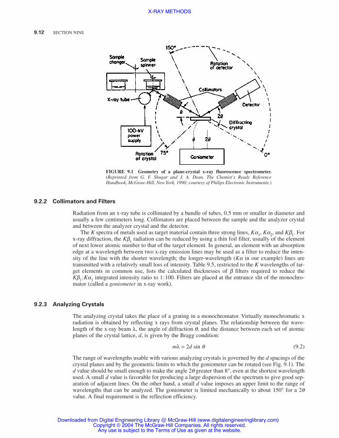
9.2.2 Collimators and Filters

Radiation from an x-ray tube is collimated by a bundle of tubes, 0.5 mm or smaller in diameter andusually a few centimeters long. Collimators are placed between the sample and the analyzer crystaland between the analyzer crystal and the detector.

The K spectra of metals used as target material contain three strong lines, Ka1, Ka2, and Kb1. Forx-ray diffraction, the Kb1 radiation can be reduced by using a thin foil filter, usually of the elementof next lower atomic number to that of the target element. In general, an element with an absorptionedge at a wavelength between two x-ray emission lines may be used as a filter to reduce the inten-sity of the line with the shorter wavelength; the longer-wavelength (Ka in our example) lines aretransmitted with a relatively small loss of intensity. Table 9.5, restricted to the K wavelengths of tar-get elements in common use, lists the calculated thicknesses of b filters required to reduce theKb1:Ka1 integrated intensity ratio to 1:100. Filters are placed at the entrance slit of the monochro-mator (called a goniometer in x-ray work).

9.2.3 Analyzing Crystals

The analyzing crystal takes the place of a grating in a monochromator. Virtually monochromatic xradiation is obtained by reflecting x rays from crystal planes. The relationship between the wave-length of the x-ray beam λ, the angle of diffraction q, and the distance between each set of atomicplanes of the crystal lattice, d, is given by the Bragg condition:

mλ = 2d sin q (9.2)

The range of wavelengths usable with various analyzing crystals is governed by the d spacings of thecrystal planes and by the geometric limits to which the goniometer can be rotated (see Fig. 9.1). Thed value should be small enough to make the angle 2q greater than 8°, even at the shortest wavelengthused. A small d value is favorable for producing a large dispersion of the spectrum to give good sep-aration of adjacent lines. On the other hand, a small d value imposes an upper limit to the range ofwavelengths that can be analyzed. The goniometer is limited mechanically to about 150° for a 2qvalue. A final requirement is the reflection efficiency.

9.12 SECTION NINE

FIGURE 9.1 Geometry of a plane-crystal x-ray fluorescence spectrometer.(Reprinted from G. F. Shugar and J. A. Dean, The Chemist’s Ready ReferenceHandbook, McGraw-Hill, New York, 1990; courtesy of Philips Electronic Instruments.)



X-RAY METHODS

Lithium fluoride is the optimum crystal for all wavelengths less than 3 Å. Pentaerythritol and potas-sium hydrogen phthalate are the crystals of choice for wavelengths from 3 to 20 Å. The long-wave-length analyzers are prepared by dipping an optical flat into the film of the metal fatty acid about 50times to produce a layer of 180 molecules in thickness. Table 9.6 gives a list of crystals commonly used.

X-RAY METHODS 9.13

TABLE 9.5 � Filters for Common Target Elements

Kb1 Ka1 = 1/100

Target Excitation Thickness, % Losselement K −a, Å voltage, keV Absorber mm g/cm2 Ka1

Ag 0.560834 25.52 Pd 0.062 0.074 60Mo 0.71069 20.00 Zr 0.081 0.053 57Cu 1.54178 8.981 Ni 0.015 0.013 45Ni 1.65912 8.331 Co 0.013 0.011 42Co 1.79021 7.709 Fe 0.012 0.009 39Fe 1.93728 7.111 Mn 0.011 0.008 38

MnO2 0.026 0.013 45Cr 2.29092 5.989 V 0.011 0.007 37

V2O5 0.036 0.012 48

Lb1 La1 = 1/100

Target Thickness, % Losselement La1 Absorber mm g/cm2 La1

W 1.4763 10.200 Cu 0.035 77


TABLE 9.6 Analyzing Crystals for X-Ray Spectroscopy

Reflecting 2d Spacing,Crystal plane Å Reflectivity

Quartz 5052�

1.624 LowAluminum 111 2.338 HighTopaz 303 2.712 MediumQuartz 202

�3 2.750 Low

Lithium fluoride 220 2.848 HighSilicon 111 3.135 HighQuartz 112 3.636 MediumLithium fluoride 200 4.028 HighSodium chloride 200 5.639 HighCalcium fluoride 111 6.32 HighQuartz 101

�1 6.686 High

Quartz 101�

0 8.50 MediumPentaerythritol (PET) 002 8.742 HighEthylenediamine tartrate (EDT) 020 8.808 MediumAmmonium dihydrogen phosphate (ADP) 110 10.648 LowGypsum 020 15.185 MediumMica 002 19.92 LowPotassium hydrogen phthalate (KAP) 101

�1 26.4 Medium

Lead palmitate 45.6Strontium behenate 61.3Lead stearate 100.4 Medium




X-RAY METHODS

9.3 DETECTORS

9.3.1 Proportional Counters

A proportional counter consists of a central wire anode surrounded by a cylindrical cathode. The twoelectrodes are enclosed in a gastight envelope typically filled to a pressure of 80 torr of argon plus20 torr of methane of ethanol (or 0.08 torr of chlorine). Radiation enters a thin window of mica,about 2 to 3 mg ⋅cm−2 thick. For work at very long wavelengths, typical window materials are 1-mmaluminum screen dipped in Formvar (usable for sodium and magnesium x rays) and 1-mm castFormvar or collodion films for oxygen, nitrogen, and boron x rays.

Each ionizing particle that enters the active volume of the counter collides with the filling gas toproduce an ion pair (argon cation plus an electron). Under the influence of a potential gradient of300 to 600 V applied across the electrodes, the initial electron soon acquires sufficient velocity toproduce a new pair of ions upon collision with another atom of argon. This gives rise to an avalancheof electrons traveling toward the central anode. The output pulse is proportional to the number of pri-mary pairs produced by the original ionizing particle.

The positive ions, if allowed to reach the cathode, would produce photons that would initiate afresh discharge. Because the methane, ethanol, or halogen gas molecules have a lower ionizationpotential than argon, after a few collisions the ions moving toward the cathode consist of only theselower-energy particle that are unable to produce photons. When the organic filling-gas ions are dis-charged at the cathode, they decompose into various molecular fragments, and eventually thequenching gas is exhausted. Counter life is limited to about 1010 counts. Because chlorine atomsmerely recombine, a halogen-quenched counter has a life in excess of 1013 counts.

The dead time, the time during which the counter will not respond to an entrant ionizing particle,is about 250 ns. Count rates up to 200 000 counts per second are possible; the upper limit is imposedby the associated electronic circuitry. About 30 eV is required for the production of an ion pair inthis detector.

9.3.2 Scintillation Counters

Certain substances (called scintillators, phosphors, or fluors) will emit a pulse of visible light or near-ultraviolet radiation when they are subjected to x radiation. The light is observed by a photomulti-plier tube (with light-amplification stages); the combination is called a scintillation counter. For xradiation a sodium iodide crystal doped with 1% thallium(I) is the best scintillator. When such radi-ation interacts with a NaI(Tl) crystal, iodine atoms are excited. Upon their return to the ground state,the reemitted ultraviolet radiation pulse is promptly absorbed by the thallium atom and, in turn,reemitted as fluorescent light at 410 nm (near the optimum wavelength response of a blue-sensitivephotomultiplier tube). The crystal is sealed within an enclosure of aluminum foil that protects thecrystal from atmospheric moisture and also serves as an internal reflector.

Dead time is 250 ns. Response is proportional to the energy of the x radiation; 500 eV is requiredto produce a photoelectron. The scintillation counter is usable throughout the important x-ray region,0.3 to 2.4 Å, and possibly up to 4 Å.

9.3.3 Lithium-Drifted Semiconductor Detectors

The lithium-drifted germanium detector consists of a virtually windowless (Ge–Li) crystal, a vacuumcryostat maintained by cryosorption pumping, a liquid-nitrogen Dewar, and a preamplifier. Use ofan electrically cooled detector (Peltier effect) eliminates the need for liquid nitrogen and allows thespectrometer to operate in any position. The solid-state Ge(Li) and Si(Li) detectors can be consid-ered as a layered structure in which a lithium-diffused active region separates a p-type entry sidefrom an n-type side. Detectors are fabricated by drifting lithium ions (a donor) into and through p-typegermanium or silicon until only a layer of p-type material remains. All acceptors within the bulk

9.14 SECTION NINE



X-RAY METHODS

material are compensated and this high-resistivity (or intrinsic) region becomes the radiation-sensi-tive region. Under reversed bias of approximately 800 to 1000 V, the active region serves as an insu-lator with an electric field gradient throughout its volume. When x radiation enters the intrinsicregion, photoionization occurs with an electron–hole pair created for each 3.8 eV of photon energyfor Si(Li) and 2.65 eV of photon energy for Ge(Li). The charge produced is rapidly collected underthe influence of the bias voltage. The detector must be maintained at 77 K at all times (unlessextremely pure germanium crystals, a recent development, are used). The charge collected each timean x-ray photon enters the detector is converted into a digital value representing the photon energy,which is interpreted as a memory address by a computer.

Silicon semiconductor detectors are preferred for x rays longer than 0.3 Å. For shorter wave-lengths, Ge detectors are necessary since Si cannot absorb the x rays effectively because the avail-able crystals are not deep enough. The response time is about 10 ns.

9.3.4 Comparison of X-Ray Detectors

For a given amount of energy absorbed, about 10 times as many electron–hole pairs are formed insolid-state Ge(Li) or Si(Li) detectors as the number of ion pairs in a gas proportional counter, andabout 170 times as many electron–hole pairs as photoelectrons in NaI(Tl) scintillation counters.Since the relative resolution of a detector is proportional to the square root of the signal, the resolu-tion of the Ge(Li) detector is about a factor of 13 better than the NaI(Tl) detector and 3 times betterthan a gas proportional counter.

9.4 PULSE-HEIGHT DISCRIMINATION

The measurement of pulse height provides the analyst with a tool for energy discrimination. Themethod is applicable whenever the amplitude of the pulse from an x-ray detector is proportional tothe energy dissipation in the detector. All three types of detectors described meet this requirement.

To operate a pulse-height amplifier, the amplifier is adjusted to produce voltage output pluses ofsuitable magnitude. The pluses are then sorted into groups according to their pulse heights. The base-line discriminator is set to pass only those pulses above a certain amplitude. Finally, the second dis-criminator (variously called the window width, the channel width, or the acceptance slit) is adjustedto reject all pulses above the sum of the baseline discriminator and the acceptance slit. Only thepluses within the confines of these two discriminator settings pass on to the counting stages. A Si(Li)or Ge(Li) detector, because of its narrow pulse-amplitude discrimination, can discriminate (resolve)between elements one or two atomic numbers apart. The pulse-height analyzer serves, in effect, as asecondary monochromator. This process permits the accumulation of an emission spectrum and itssubsequent display on a video screen.

An auxiliary electronic circuit, called the pulse pile-up rejection circuit, prevents charge collec-tion from multiple photons that enter in rapid succession.

9.5 X-RAY ABSORPTION METHODS

9.5.1 Principle

Although complex experimental equipment is required, measurement in x-ray absorption methods isstraightforward. Radiation traversing a layer of substance is diminished in intensity by a constantfraction per centimeter thickness x of material. The emergent radiant power P, in terms of incidentradiant power P0, is given by

P = P0 exp(−mx) (9.3)

X-RAY METHODS 9.15



X-RAY METHODS

9.16 SECTION NINE

which defines the total linear absorption coefficient m. Since the reduction of intensity is deter-mined by the quantity of matter traversed by the primary beam, the absorber thickness is bestexpressed on a mass basis, in g ⋅ cm2. The mass absorption coefficient m /r, expressed in unitscm2 ⋅g, where r is the density of the material, is approximately independent of the physical stateof the material and, to a good approximation, is additive with respect to the elements composinga substance.

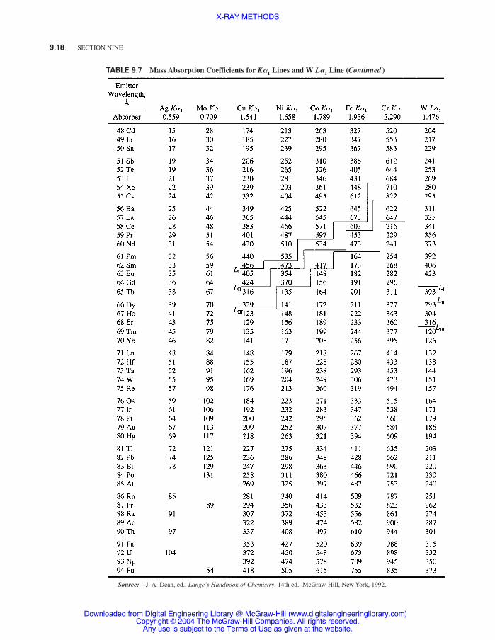
Table 9.7 contains values of m /r for the common target elements employed in x-ray work. A moreextensive set of mass absorption coefficients for K, L, and M emission lines within the wavelengthrange from 0.7 to 12 Å is contained in Ref. 2.

In x-ray absorption work the specimen is irradiated with two or more monochromatic x rayswhile the incident (P0) and transmitted (P) radiant energies are monitored. Because only one elementhas changed its mass absorption coefficient at an absorption edge, this relationship pertains:

(9.4)

where the term in parentheses represents the difference in mass absorption coefficient at the edgediscontinuity, W is the weight fraction of the element, and the product rx is the mass thickness of thesample in grams per square centimeter. There is no matrix effect, which gives the absorption methodan advantage over x-ray fluorescence analysis in some cases.

In contrast to absorption measurements in other portions of the electromagnetic spectrum,only a single attenuation measurement is made on each side of the edge because spectrometersthat provide a continuously variable wavelength of x radiation are not commercially available.Instead, two x-ray emission lines are used for each edge. Primary excitation from an x-ray tubestrikes a target. For example, a crystal of SrCO3 would provide the Sr Ka1 line and a crystal ofRbCl would provide the Rb Ka1 line. The Sr line lies on the short-wavelength side of the Br Kedge and the Rb line on the long-wavelength side of the edge. After suitable standards have beenrun to calibrate the equipment, bromine can be determined in various materials such as dibro-moethane in gasolines.

For the light elements whose valence electrons may be involved in x-ray absorption, the exactposition of the absorption edge (fine structure) can give the oxidation state of the atom in question.

9.5.2 Radiography

The gross structure of various types of specimens may be examined by absorption techniques usingrelatively simple equipment. The microradiographic camera fits as an inset in the collimating systemof commercial x-ray equipment. Photographic film with an extremely fine grain makes magnifica-tion up to 200 times possible. Sample thicknesses vary from a few hundredths to a few tenths of amillimeter; only a few seconds of exposure are necessary.

9.6 X-RAY FLUORESCENCE METHOD

9.6.1 Principle

When a sample is bombarded by a beam of x radiation that contains wavelengths shorter than theabsorption edge of the spectral lines desired, characteristic secondary fluorescent x-ray spectra areemitted. The atom is in a highly excited state after such photoelectric absorption. An electronjumps from a higher to the lower shell to fill that vacancy emitting an x-ray photon. These x-rays

2 30

. log ( )P

PW x= ′′ − ′m m r

2 K. F. J. Heinrich, in T. D. McKinley, K. F. J. Heinrich, and D. B. Wittry, eds., The Electron Microprobe, Wiley, New York,1966, pp. 351–377.



X-RAY METHODS

X-RAY METHODS 9.17

TABLE 9.7 Mass Absorption Coefficients for K�1 Lines and W L�1 Line

(Continued)



X-RAY METHODS

9.18 SECTION NINE

TABLE 9.7 Mass Absorption Coefficients for K�1 Lines and W L�1 Line (Continued )




X-RAY METHODS

are characteristic of an element as the energy or wavelength is different for each element. Besides x rays, electron bombardment is used in the scanning electron microscope and the electron micro-probe. Certain radionuclides are x-ray emitters and can be used as excitation sources, particularly inportable equipment.

The x-ray fluorescence method rivals the accuracy of wet chemical techniques in the analysis ofmajor constituents. However, for trace analyses, it is difficult to detect an element present in less thanone part in 10 000. In absolute terms the limit is about 10 ng. The method is attractive for elementsthat lack reliable wet chemical methods and for the analysis of nonmetallic specimens. X-ray fluo-rescence is one of the few techniques that offers the possibility of quantitative determinations withabout 5% to 10% relative error without the use of a suite of standards. X-ray fluorescence methodallows direct analysis of an element in solid substances.

9.6.2 Instrumentation

The general arrangement for exciting, dispersing, and detecting fluorescent radiation with a plane-crystal spectrometer is shown in Fig. 9.1. The sample is irradiated with an unfiltered beam of pri-mary x rays. A portion of the fluorescence x radiation is collimated by the entrance slit of thegoniometer and directed onto the surface of the analyzing crystal. The radiations reflected accordingto the Bragg condition [Eq. (9.2)] pass through the exit collimator to the detector.

For elements of atomic number less than 21, a vacuum of 0.1 torr is needed or the system mustbe flushed with helium. Below magnesium (atomic number 12) the transmission becomes seriouslyattenuated.

9.6.3 Sample Handling

Samples are best handled as liquids if they can be conveniently dissolved. Sample depth should beat least 5 mm so that the sample will appear infinitely thick to the primary x-ray beam. If possible,solvents that do not contain heavy atoms should be used. Water and nitric acid are superior tohydrochloric or sulfuric acid. Powders are best converted into a solid solution by fusion withlithium borate (both light elements). Powders can also be pressed into a wafer but should be heavilydiluted with a material that has a low absorption, such as powdered starch, lithium carbonate, lamp-black, or gum arabic to avoid matrix effects (as done by a borax fusion).

9.6.4 Matrix Effects

Matrix effects arise from the interaction of elements in the sample to affect the x-ray emission inten-sity in a nonlinear manner. They are often negligible when thin samples, which may be collected ona filter, mesh, or membrane, are used for analyses. The most practical way to correct for matrixeffects is to use the internal standard technique. Even so, this technique is only valid if the matrixelements affect the reference line and analytical line in exactly the same way. The following list pre-sents the potential problems:

1. If a disturbing element has an absorption edge between the comparison lines, preferential absorp-tion of the line on the short-wavelength side of the edge will occur.

2. If fluorescence from a matrix line lies between the absorption edges of the analytical and refer-ence elements, selective enhancement results for the element whose absorption edge lies at thelonger wavelength.

3. Line intensity can be enhanced if a matrix element absorbs primary radiation and then, by fluo-rescence, emits radiation that in turn is absorbed by a sample element and causes that latter to flu-oresce more strongly.

X-RAY METHODS 9.19



X-RAY METHODS

9.7 ENERGY-DISPERSIVE X-RAY SPECTROMETRY

Energy-dispersive x-ray spectrometry differs from x-ray fluorescence in that x rays emitted from ele-ments in the sample are observed by a solid-state detector and pulse-height analyzer without usinga crystal analyzer and collimators with their attendant energy losses. Equipment is very compact.Computer-based multichannel analyzers are then used to acquire a spectrum of counts versus energyand to perform data analysis. As this information is being collated, it can be simultaneously dis-played as a spectrum on a video screen. Computer-generated emission lines can be superimposed onthe spectrum displayed. Often elements can be identified by the line positions alone. When overlapof the emission lines from one or more elements may be possible, one should use the relative inten-sities of the lines as well as their positions to confirm the elemental identification. Detection limitsin bulk material are typically a few parts per million.

Energy-dispersive x-ray spectrometry offers the advantage of being a simultaneous multielementmethod for samples with elements separated by one or two atomic numbers. Quantitative determi-nations can range from the use of simple intensity–concentration standard working curves to com-puter programs that convert intensity to concentration. Emission lines that have no spectral overlapcan be measured from a spectrum using software to perform integration of the net peak intensityabove the background for the peak of interest. Cases in which peak overlap is of concern requirespectrum-fitting techniques from a library of reference spectra. Care must be taken to maintain theaccuracy of the energy calibration of the instrumentation.

Primary x-ray tubes are operated at low power and can be air-cooled. The tube anode material is usu-ally Rh, Ag, or Mo. A filter wheel, typically fitted with six filters, is located between the tube and the sam-ple. The x-ray tube can also be focused on secondary targets to produce specific fluorescent x-ray lines.

Portable instruments are designed around x rays emitted from a radionuclide source. A variety ofisotopes is needed to provide radiation over the energy range needed.

Unfortunately, the resolution of an energy-dispersion instrument is as much as 50 times less thanthe wavelength-dispersion spectrometer using a crystal analyzer. For precise quantitative measure-ments, wavelength dispersion followed by energy-dispersive detectors and pulse-height analyzersmust be used to get sufficient resolution.

9.8 ELECTRON-PROBE MICROANALYSIS

When materials are bombarded by a high-energy electron beam, as in an electron microscope, x-rayfluorescence radiation is produced. By incorporating an x-ray fluorescence spectrometer directly intothe instrument, it is possible to obtain the same sort of elemental data as obtained by normal x-rayfluorescence directly on the area viewed or scanned by the electron beam. It is possible to obtain quali-tative and quantitative elemental data from a volume of 0.1 mm3 for elements of atomic number 5 (boron)and higher. When the electron beam is scanned across the sample, a point-by-point spatial distributionof elements across the surface (or area) of the sample is produced. Excitation is restricted to thin surfacelayers because the electron beam penetrates to a depth of only 1 or 2 mm into the specimen.

The electron optical system consists of an electron gun followed by two electromagnetic focus-ing lenses to form the electron-beam probe. The specimen is mounted as the target inside the high-vacuum column of the instrument. If not conductive, the surface of the specimen must be treated witha coating to make its surface conductive in order to avoid the problems of specimen charging withelectron bombardment.

9.9 ELECTRON SPECTROSCOPY FOR CHEMICAL APPLICATIONS (ESCA)

Electron spectroscopy for chemical applications, or x-ray photoelectron spectroscopy (XPS), is a nonde-structive spectroscopic tool for studying the surfaces of solids. Any solid material can be studied and allelements (except hydrogen) can be detected by this technique, usually at 0.1 atomic percent abundance.

9.20 SECTION NINE



X-RAY METHODS

9.9.1 Principle

When a specimen is exposed to a flux of x-ray photons of known energy, all electrons whose bind-ing energies Eb are less than the energy of the exciting x rays are ejected. The kinetic energies Ekinof these photoelectrons are then measured by an energy analyzer in a high-resolution electron spec-trometer. For a free molecule or atom, conservation of energy requires that

Eb = hn − Ekin − f (9.5)

where hn is the energy of the exciting radiation and f is the spectrometer work function, a constantfor a given analyzer. The binding energy is indicative of a specific element and a particular structuralfeature of electron distribution.

9.9.2 Chemical Shifts

The binding energies of core electrons are affected by the valence electrons and therefore by thechemical environment of the atom. Chemical shifts, as they are called, are observed for every ele-ment except hydrogen and helium. Applicability to carbon, nitrogen, and oxygen makes ESCA animportant structural tool for organic materials. In general, the ESCA chemical shifts lie in the range0 to 1500 eV; peak widths vary from 1 to 3 eV. To make assignments, one must refer to a catalog ofelement reference spectra or to correlation charts.

9.9.3 ESCA Instrumentation

Instrumentation for ESCA involves (1) a source of soft x rays, usually Mg Ka1,2 and Al Ka1,2,(2) a device that collects the emitted electrons, counts them, and carefully measures their kineticenergy (an energy analyzer), and (3) a vacuum system capable of providing an operating pres-sure of about 5 × 10−6 torr. Samples must be low-pressure solids or liquids condensed onto acryogenic probe. The two alternative sources are needed to distinguish ESCA peaks from Augerpeaks. When a different x-ray source is used, the ESCA peaks shift in kinetic energy but thekinetic energies of Auger peaks remain constant and appear at the same energy position in thespectrum.

One type of ESCA spectrometer places the x-ray anode, a spherically bent crystal disperser, andthe sample on a Rowland circle. In the energy analyzer an electrostatic field sorts the electrons bytheir kinetic energies and focuses them at the detector. A continuous channel electron multipliercounts the electrons at each step as the electrostatic field is increased in a series of small steps. A plotof the counting rate as a function of the focusing field gives the spectrum.

9.9.4 Uses

The intensity of a photoelectron line is proportional not only to the photoelectric cross section of aparticular element but also to the number of atoms of that particular element present in the sample.Analyses of mixtures are often accurate to ±2%.

Because of the unique ability of ESCA to study surfaces, the technique is used to study hetero-geneous catalysts, polymers and polymer adhesion problems, and materials such as metals, alloys,and semiconductors. The probe depth is 1 to 2 nm.

9.10 AUGER EMISSION SPECTROSCOPY (AES)

Once an atom is ionized, it must relax by emitting either an x-ray photon or an electron. The latteris the nonradiative Auger process that nature chooses in most instances, and, increasingly so, for ele-ments of atomic number less than 30. A combination unit involves an electron gun centered with an

X-RAY METHODS 9.21



X-RAY METHODS

energy analyzer unit. The electron gun is focused on the sample; the detector is at the opposite endof the energy analyzer.

A KLL Auger transition involves these processes: A K electron undergoes the initial ionization.An L-level electron moves in to fill the K-level vacancy and, at the same time, gives up the energyof that transition to another L-level electron. The latter becomes the ejected Auger electron. Theenergy of the ejected electron is a function only of the atomic energy levels involved in the Augertransition and is thus characteristic of the atom from which it came. Most elements have more thanone intense Auger peak; LMM and MNN are other transitions. A recording of the spectrum of ener-gies of Auger electrons released from any surface is compared with the known spectra of pure ele-ments. Typically the sampling depth is about 2 nm.

Shifts from one element to the next are about 25 eV; peak positions can be measured to an accu-racy of ±1 eV. Spectra of all the elements lie between 50 and 1000 eV. Both qualitative and quanti-tative analyses of the elements in the immediate surface atomic layers are possible with Augeremission spectroscopy. When combined with a controlled removal of surface layers by ion sputter-ing, AES provides the means to solve some very important problems involving surfaces.

9.11 X-RAY DIFFRACTION

9.11.1 Principle

When a beam of monochromatic x radiation is directed at a crystalline material, one observes reflectionor diffraction of the x rays at various angles with respect to the primary beam. The relationship betweenthe wavelength of the x radiation, the angle of diffraction, and the distance between each set of atomicplanes of the crystal lattice is given by the Bragg condition [Eq. (9.2)]. From the Bragg condition onecan calculate the interplanar distances of the crystalline material. The interplanar spacings depend solelyon the geometry of the crystal’s unit cell while the intensities of the diffracted x rays depend on the typeof atoms in the crystal and the location of the atoms in the fundamental repetitive unit, the unit cell.

From the rearranged Bragg equation

(9.6)

the two factors within the parentheses control the choice of x radiation. Because the parentheticalterm cannot exceed unity, the use of long-wavelength radiation limits the number of reflections thatare observed, whereas short-wavelength radiation tends to crowd individual reflections very closetogether. Furthermore, radiation just shorter in wavelength than the absorption edge of an element inthe specimen should be avoided because the resulting fluorescent radiation increases the back-ground. For these reasons, a multiwindow x-ray tube with anodes of Ag, Mo, W, and Cu is used.

Diffractometer alignment procedures require the use of a well-prepared polycrystalline specimen. Twostandard samples found to be suitable are silicon and a-quartz (including Novaculite). The 2q values ofseveral of the most intense reflections for these materials are listed in Table 9.8. To convert to d for aver-age K −a values or to d for Ka2, multiply the tabulated d value (Table 9.8) for Ka1 by the factor given below:

Element K −a (average) Ka2

W 1.007 69 1.023 07Ag 1.002 63 1.007 89Mo 1.002 02 1.006 04Cu 1.000 82 1.002 48Ni 1.000 77 1.002 32Co 1.000 77 1.002 16Fe 1.000 67 1.002 04Cr 1.000 57 1.001 70

q =

−sin 1

2

λd

9.22 SECTION NINE



X-RAY METHODS

9.23

TA

BLE

9.8

Inte

rpla

nar

Spac

ings

for

K�

1R

adia

tion

,dve

rsus

2�

a-Q

uart

z (i

nclu

ding

nov

acul

ite)

hkl

100

101

110

102

200

112

202

211

203

301

d, Å

4.26

03.

343

2.45

82.

282

2.12

81.

817

1.67

21.

541

1.37

51.

372

WKa 1

: 2q

2.81

3.58

4.87

5.25

5.63

6.59

7.17

7.78

8.72

8.74

Ag

Ka 1

: 2q

7.53

9.60

13.0

714

.08

15.1

017

.71

19.2

620

.91

23.4

723

.52

Mo

Ka 1

: 2q

9.55

12.1

816

.59

17.8

819

.19

22.5

124

.49

26.6

129

.89

29.9

6C

uKa 1

: 2q

20.8

326

.64

36.5

239

.45

42.4

450

.16

54.8

659

.98

68.1

468

.31

Ni

Ka 1

: 2q

22.4

428

.71

39.4

242

.60

45.8

554

.28

59.4

465

.08

74.1

574

.34

Co

Ka 1

: 2q

24.2

431

.04

42.6

846

.15

49.7

158

.98

64.6

870

.96

81.1

681

.38

FeKa 1

: 2q

26.2

733

.66

46.3

850

.20

54.1

164

.38

70.7

577

.83

89.5

089

.74

Cr

Ka 1

: 2q

31.1

840

.05

55.5

260

.22

65.0

978

.11

86.4

295

.96

112.

7311

3.11

Silic

on

hkl

111

220

311

400

331

422

511.

333

440

531

620

d, Å

3.13

531.

9199

71.

6373

61.

3576

301.

2458

41.

1085

1.04

510.

0959

986

0.91

7922

0.85

8637

WKa 1

: 2q

3.82

6.24

7.32

8.83

9.62

10.8

211

.48

12.5

013

.07

13.9

8A

gKa 1

: 2q

10.2

416

.75

19.6

723

.78

25.9

529

.23

31.0

433

.88

35.4

838

.02

Mo

Ka 1

: 2q

12.9

921

.29

25.0

230

.28

33.0

837

.32

39.6

743

.36

45.4

548

.79

Cu

Ka 1

: 2q

28.4

447

.30

56.1

269

.13

76.3

888

.03

94.9

610

6.71

114.

1012

7.55

Ni

Ka 1

: 2q

30.6

651

.16

60.8

375

.26

83.4

296

.80

104.

9611

9.42

129.

1214

9.76

Co

Ka 1

: 2q

33.1

555

.53

66.2

282

.42

91.7

710

7.59

117.

7113

7.42

154.

04Fe

Ka 1

: 2q

35.9

760

.55

72.4

890

.96

101.

9712

1.67

135.

70C

rKa 1

: 2q

42.8

373

.21

88.7

211

4.97

133.

53

Sour

ce:

Tabl

es o

f In

terp

lana

r Sp

acin

gs d

vs.

Diff

ract

ion

Ang

le 2q

for

Sele

cted

Tar

gets

, Pic

ker

Nuc

lear

, Whi

te P

lain

s, N

Y, 1

966.



X-RAY METHODS

The applications of x-ray diffraction can be conveniently considered under three main headings:powder diffraction, polymer characterization, and single-crystal structure studies. In addition thereare many specialized uses.

9.11.2 Powder Diffraction

In the powder method, the sample is a large collection of very small crystals, randomly oriented. Apolycrystalline aggregate is formed into a cylinder whose diameter is smaller than the diameter ofthe incident x-ray beam. The diffraction pattern in a series of nonuniformly spaced cones (as inter-cepted on the photographic film) whose spacings are determined by the prominent planes of thecrystallites.

Metal samples may be machined to a cylindrical configuration, plastic materials can often beextruded through suitable dies, and all other samples are best ground to a fine powder (200 to 300mesh) and shaped into thin rods after mixing with collodion binder or simply tamped into a uniformglass capillary. Liquids must be converted into crystalline derivatives.

The x-ray pattern of a pure crystalline substance can be considered as a “fingerprint” with eachcrystalline material having, within limits, a unique diffraction pattern. The ASTM has published thepowder diffraction patterns of some 50 000 compounds. An identification of an unknown compoundis made by comparing the interplanar spacings of the powder pattern of a sample to the compoundsin the ASTM file. The d value for the most intense line of the unknown is looked up first in the file.In a single compound, the d values of the next two most intense lines are matched against the filevalues. After a suitable match for one component is obtained, all the lines of the identified compo-nent are omitted from further consideration. The intensities of the remaining lines are rescaled bysetting the strongest intensity equal to 100 and repeating the entire procedure. If x-ray fluorescencedata are also added, the comparison is even more definitive. A systematic search, either manual orby computer, usually leads to an identification within an hour. Mixtures of up to nine compounds canoften be completely identified. The minimum limit of detection is about 1% to 2% of a single phase.

In addition to identifying the compounds in a powder, the diffraction pattern can also be used todetermine the degree of crystalline disorder, crystalline size, texture, and other parameters associatedwith the state of the crystalline materials. Differentiation among various oxides such as MnO,Mn2O3, MnO2, and Mn3O4, or between materials present in such mixtures as NaCl + KBr or KCl +NaBr, is easily accomplished by x-ray diffraction. Identification of various hydrates, such asNa2CO3 ⋅H2O and Na2CO3 ⋅10H2O, is another application.

9.11.3 Polymer Characterization

The following information can be obtained from wide-angle and small-angle x-ray studies of poly-mers:

1. Degree of crystallinity

2. Crystallite size

3. Degree and type of preferred orientation

4. Polymorphism

5. Microdiffraction patterns

6. Information concerning the macrolattice of the crystallites

Fibers and partially oriented samples show spotty diffraction patterns rather than uniform cones;the more oriented the specimen, the spottier the pattern. The degree of crystallinity and crystallitesize can be measured in powders, films, and fibers. This determination usually takes a few hours.The degree of orientation in uniaxially oriented materials, such as fibers, can also be determined in

9.24 SECTION NINE



X-RAY METHODS

a few hours. If the orientation is other than uniaxial, the type of orientation and an approximate deter-mination of the degree of orientation require similar times.

Polymorphism, the phenomenon in which a chemical compound can exist in more than one crys-talline form, is often exhibited by polymers. From a study of the diffraction pattern, the presence ofpolymorphism can be ascertained and the approximate percentages of the polymorphs presentdetermined. Such a study usually requires 1 to 2 days.

Micro x-ray diffraction can be used to identify inclusions in polymers and other materials. It canalso be used to study the relationship of the skin of fibers to their interiors in regard to crystallinity,crystallite size, and orientation. Areas as small as 25 mm2 can be studied. One limitation is that thespecimen must be transparent to the x-ray beam. For most materials, a thickness up to 1 mm can betolerated. Studies require 1 to 2 days.

Small-angle x-ray scattering is used to obtain information about the macrolattice, which can bedefined as a periodic array of matter in space that is greater than 5.0 nm in size. In many polymersthe chains fold back on themselves, forming crystallites. This leads to crystalline and amorphousdomains ranging in size from less than 10 nm to almost 100 nm. Small-angle scattering studies areused to determine the size, distribution, and orientation of these domains.

9.11.4 Single-Crystal Structure Determination

Three-dimensional molecular structures can be determined using single-crystal x-ray diffraction pro-cedures. The structures of molecules of considerable complexity (up to about 100 atoms) can becompletely elucidated. In addition to the chemical structure, a crystal determination reveals the con-figuration and conformation of the molecule in the solid state.

The crystal, less than 1 mm in size, is affixed to a thin glass capillary (with shellac) that in turnis fastened to a brass pin that is mounted in the x-ray diffraction unit. In the rotating-crystal method,monochromatic x radiation is incident on the crystal that is rotated about one of its axes. Thereflected beams lie as spots on the surface of cones that are coaxial with the rotation axis.

Bibliography

Bertin, E. P., Principles and Practice of X-Ray Spectrometric Analysis, 2d ed., Plenum, New York, 1978.Jenkins, R., R. W. Gould, and D. Gedcke, Quantitative X-Ray Spectrometry, Dekker, New York, 1981.Tertian, R., and F. Claisse, Principles of Quantitative X-Ray Fluorescence Analysis, Heyden, London, 1982.Thompson, M., M. D. Baker, A. Christie, and J. F. Tyson, “Auger Emission Spectroscopy,” in Vol. 74 ofChemical Analysis, Wiley, New York, 1985.

X-RAY METHODS 9.25



X-RAY METHODS

x ray methods

Science

xray methods

monochromatic xray beam

electron spectroscopy

xray absorp tion

ejected electron

inner electron levels

electronprobe microanalysis

electron probe microanalysis