Xiaoyun ZhangAssociate Professor

School of Mechanical Engineering,

Shanghai Jiaotong University,

909 Mechanical Building,

800 Dong Chuan Road,

Shanghai 200240, China

e-mail: general_zhang@sjtu.edu.cn

Zhen HuResearch Assistant

e-mail: zh4hd@mst.edu

Xiaoping Du1

Associate Professor

e-mail: dux@mst.edu

Department of Mechanical

and Aerospace Engineering,

Missouri University of Science and Technology,

290D Toomey Hall,

400 West 13th Street,

Rolla, MO 65409-0500

Probabilistic Inverse Simulationand Its Application in VehicleAccident ReconstructionInverse simulation is an inverse process of direct simulation. It determines unknowninput variables of the direct simulation for a given set of simulation output variables.Uncertainties usually exist, making it difficult to solve inverse simulation problems. Theobjective of this research is to account for uncertainties in inverse simulation in orderto produce high confidence in simulation results. The major approach is the use of themaximum probability density function (PDF), which determines not only unknown deter-ministic input variables but also the realizations of random input variables. Both typesof variables are solved on the condition that the joint probability density of all the ran-dom variables is maximum. The proposed methodology is applied to a traffic accidentreconstruction problem where the simulation output (accident consequences) is knownand the simulation input (velocities of the vehicle at the beginning of crash) is sought.[DOI: 10.1115/1.4025296]

Keywords: inverse simulation, maximum probability, accident reconstruction,optimization

1 Introduction

Inverse simulation is an inverse process of direct simulation.During this process, computer simulations are used in an inverseway. A set of unknown model input variables are found given aset of known model output variables.

Inverse simulation has been applied in many engineering areas.For instance, it is extensively used and becomes a current researchfocus in the area of inverse dynamic analysis, such as determiningthe forces or torques so as to produce desired motions [1,2], findingappropriate joint parameters for robots [3], and determining tor-ques and powers for desired human movements [4–7]. The applica-tions in aerospace engineering have also been reported, such asdynamic inversion [8], flight control [9,10], optimization of heli-copter slalom maneuver [11], and other applications [12–14].

Even though inverse simulations are intensively used forinverse dynamic analysis, they are not limited to dynamic analy-sis. Traffic accident reconstruction, which is the focus of thiswork, is another area to which inverse simulations are applied. Itis different from the traditional inverse dynamics where the num-ber of to-be-determined input variables, which enforce a dynami-cal system to complete the specified output, is generally equal tothe number of dynamic equations. For the accident reconstructioninverse simulation, the number of unknowns may be differentfrom that of simulation equations. Some of the input variables,such as the coefficient of friction, are not known exactly. Thesevariables together with the totally unknown input variables, suchas the pre-impact velocity, are determined by optimization so thatthe direct simulation result is close to observations. Details aboutthe inverse simulation of traffic accident reconstruction are dis-cussed in Sec. 2.

Figure 1 shows a general simulation model. The vectors ofinput and output variables are x and y, respectively. x and y maybe time independent or time dependent. The simulation modelgðxÞ maps x into y and is given by

y ¼ gðxÞ (1)

ory1 ¼ g1ðxÞy2 ¼ g2ðxÞ� � �ym ¼ gmðxÞ

8>>>><>>>>:

(2)

where y ¼ ðy1;…; ymÞT, and gð�Þ ¼ ðg1ð�Þ;…gmð�ÞÞT. We callthese equations the direct simulation equations.

For inverse simulation, the output variables y are known, andpart of the input variables are to be determined. We use xunkn forthose to-be-determined variables. Some input variables areprecisely known, and we denote them by xkn.

As many uncertainties are presented in the direct process ofsimulation [15–17], we also encounter uncertainties in inversesimulation. The uncertainties may be associated with simulationparameters that are related to the stochastic physical nature, manu-facturing imprecision, random operating conditions, and measure-ment errors. As a result, we may not know some of the inputvariables precisely, and we treat them as random variables. Thoserandom variables are denoted by xrand. Model structure uncer-tainty also exists due to simplifications, assumptions, ignorance,and lack of information within the model. When we solve for theunknown input variables through inverse simulation, the modelstructure uncertainty should also be considered.

Then, the input variables x are

x ¼ ðxunkn; xrand; xknÞT (3)

wherexunkn ¼ ðxunkn; 1;…; xunkn;nunkn

ÞT with a size of nunkn,

xrand ¼ ðxrand;1; …; xrand; nrandÞT with a size of nrand.

Since the precisely known variables xkn are not important inour discussions, we omit them in the simulation models. Then, themodels are rewritten as

y ¼ gðxÞ ¼ gðxunkn; xrandÞ (4)

1Corresponding author.Contributed by the Design Automation Committee of ASME for publication in

the JOURNAL OF MECHANICAL DESIGN. Manuscript received March 25, 2013; finalmanuscript received August 19, 2013; published online September 19, 2013. Assoc.Editor: David Gorsich.

Journal of Mechanical Design DECEMBER 2013, Vol. 135 / 121006-1Copyright VC 2013 by ASME

Downloaded From: http://mechanicaldesign.asmedigitalcollection.asme.org/ on 09/23/2013 Terms of Use: http://asme.org/terms

The general task of inverse simulation is to find unknown inputvariables xunkn given output variables y and joint probabilitydensity distribution of random input variables xrand.

We then take traffic accident reconstruction as an example tofurther explain inverse simulation and its input variables xunkn andxrand. From the accident scene, we may obtain useful information,such as the victim rest position, for which we can run vehicle col-lision simulation repeatedly until the simulated human rest posi-tion matches the observed value. The human rest position servesas one of the output variables in y. On the other hand, the inputvariables may include the pre-impact velocity of the vehicle, thedistance between the pedestrian and vehicle, and the coefficient offriction. If the pre-impact velocity and the distance between thepedestrian and vehicle are what should be revealed from theinverse simulation, then they belongs to unknown input variablesxunkn. The coefficient of friction may also be unknown. If we havesufficient statistical data, we know its probability density before-hand. It can be treated as a random input variable, and then itbelongs to xrand. If it is difficult or impossible to measure the coef-ficient of friction at the accident scene, its realization can besolved during the inverse simulation. Therefore, for an accidentthat has occurred, the random variables xrand could be observed ormeasured; in other words, their realizations exist. These realiza-tions of xrand are also to-be-determined unknowns.

Due to the involvement of random variables, the traditionalinverse simulation method may not be effective anymore. In thiswork, we develop a new inverse simulation method that can deter-mine both the unknown deterministic input variables and the real-izations of unknown random input variables. The requirement ofthe method is that we know the direct simulation output variablesand the prior distributions of the random input variables.

Vehicle accident reconstruction is an important application areaof inverse simulation, and we give a brief introduction to vehicleaccident reconstruction in Sec. 2. We then present the proposedmethod in Sec. 3 followed by an illustration example in Sec. 4. Themethod is applied in the reconstruction of a vehicle–pedestrianaccident in Sec. 5. Conclusions and future work are discussed inSec. 6.

2 Vehicle Traffic Accident Reconstruction

The whole process of a vehicle accident can be divided intothree phases:

(1) Postimpact: It is the starting point of the reconstruction.The model is developed with the information obtained fromthe accident scene.

(2) Impact: It identifies the responses of the involved vehicle,including the impact speed, impact direction, impact loca-tion, and so on.

(3) Pre-impact. It identifies the speed and trajectory of the vehi-cle [18].

For traffic accident reconstruction, the key issues are the investi-gation and analysis of the causes and consequences of vehicle colli-sion. More specifically, a collision analysis is performed to identifycontributions of major factors to the collision. These factors includethe role of the drivers, vehicles, road conditions, and environment.

Traffic accident reconstruction is an inverse process of directsimulation because it reconstructs the pre-accident events giventhe accident consequences. Several computer programs have beendeveloped for the reconstruction of vehicle accidents based on theinformation of the accident scene. The commonly used accident

scene information include vehicle or human rest position, roadmarks, damages and marks of vehicle or other road infrastruc-tures, and human injuries [19]. The most typical accident recon-struction software is PC-CRASH. As the software is combined with amomentum-based collision model, the accidents can be recon-structed from the point of reaction to the end position for allinvolved cars simultaneously.

The major objective of accident reconstruction is to identify thepre-impact velocity and trajectory at the moment of accident.Elastic–plastic deformation of the vehicle and the injury of thehuman body are the important information in the vehicle crashaccidents. The computer simulation models available for the acci-dent reconstruction, however, seldom consider the deformationand the injury. With the development of simulation technology,the deformation can be fully analyzed based on the finite elementmethod or the multibody dynamics methods. The deformationanalysis plays a vital role in the reconstruction of vehicle crashaccidents. In this work, the MADYMO (mathematical dynamicmodel) is employed to study the vehicle-pedestrian impact acci-dent. MADYMO employs the multibody dynamics and injury bio-mechanics for accident simulation. It is applicable to many kindsof transportations, such as cars, motorcycles and bicycles [20]. Ituses numerical algorithms to predict the motion of systems withbodies connected by kinematic joints. It is convenient to use thedatabase of human body models developed by TNO (NetherlandsOrganization for Applied Science Research) and EEVC (Euro-pean Experimental Vehicles Committee), including the Hybrid IIIdummy and pedestrian models in this software.

As many uncertainties present in the process of direct simula-tions [16,17,21], we also face uncertainties in inverse simulations.The uncertainties may come from simulation parameters, such asthe random road conditions. They can also come from the modelstructure uncertainties in the vehicle crash simulation models dueto simplifications, assumptions, ignorance, and lack of informa-tion. For example, there are many sources of uncertainty in trafficaccident reconstruction as reported in Refs. [22,23]. The majorobjective of this work is to develop a probabilistic inverse simula-tion methodology and then use it to deal with the uncertainties inthe vehicle accident inverse simulation.

3 Inverse Simulation With Maximum Probability

Density

In this section, we present the proposed methodology forinverse simulation under uncertainty. As discussed previously, thetask is to find the unknown input variables xunkn given the outputvariables y and the joint probability density function of randominput variables xrand.

During the inverse simulation process, we need to solve thedirect simulation equations in Eq. (2), and the equations with theinput variables we defined in Sec. 1 are rewritten below

y1 ¼ g1ðxunkn; xrandÞy2 ¼ g2ðxunkn; xrandÞ� � �ym ¼ gmðxunkn; xrandÞ

8>><>>: (5)

For a special case where the dimension of y is equal to that ofxunkn, the number of equations are equal to the number ofunknown variables. Then, there may be a unique solution to xrand

given a specific set of values of y. In this case, xunkn can beobtained with a reliability approach [24]. In this work, we discussgeneral problems where the number of unknowns is greater thanthe number of simulation equations.

The distributions of random input variables xrand are usuallyobtained from statistical data, engineering judgment, and priorsimilar simulation applications. As discussed in Sec. 1, however,for a specific event under simulation, the random input variablesxrand actually become deterministic, meaning that their values are

Fig. 1 A simulation model

121006-2 / Vol. 135, DECEMBER 2013 Transactions of the ASME

Downloaded From: http://mechanicaldesign.asmedigitalcollection.asme.org/ on 09/23/2013 Terms of Use: http://asme.org/terms

no longer random. Instead, their values are fixed but maybeunknown. For example, in a vehicle accident simulation, the coef-ficient of friction lf between the tires of the vehicle and groundmight be an input random variable. When we build the simulationmodel for vehicle collision, we can treat lf as a random variablebecause we know there is uncertainty associate with lf whose dis-tribution may be known in advance. However, for a specific acci-dent, a unique true value of lf exists even though we may notknow it unless we measure it. For a specific accident event, thetrue value of lf is a realization of the random variable lf . For thisreason, the total number of unknowns in the inverse simulation isthe sum of the numbers of xunkn and xrand, or nunkn þ nrand. If thenumber of output variables ny < nunkn þ nrand, we will have aninfinite number of solutions.

To solve this problem, we need to use the prior probabilistic in-formation about the random input variables xrand, which can inturn impose conditions in addition to the direct simulation equa-tions. This may allow us to generate a unique solution. Supposethe solution to the inverse simulation is x�, the strategy we pro-pose is to produce the highest probability density for the randominput variables xrand at x�. In other words, we select a solutionamong the infinite number of solutions so that the probabilitydensity of xrand is maximum.

The new method has a number of advantages. First, it uses allthe information available. It does not simply treat xrand as unre-lated unknowns; instead, the probabilistic information of xrand isfully used, and the correlation of the elements in xrand is also con-sidered through the joint probability density of xrand and the directsimulation equations. Second, the maximum joint probability den-sity is achieved, resulting in the highest confidence in the inversesimulation result. Third, a unique solution may be obtained. Aswill be discussed next, the last advantage of the new method isthat the inverse simulation and probabilistic analysis can be inte-grated by an optimization framework, which results in an easynumerical implementation.

Let the joint PDF of xrand be f ðxrandÞ. For a special case whereall the random variables in xrand are independent, f ðxrandÞ is givenby

f ðxrandÞ ¼Ynrand

i¼1

fiðxrand;iÞ (6)

where fið�Þ is the PDF of xrand;i.Our task now is to find the unknown variables

x ¼ ðxTunkn; x

TrandÞ

Tthat maximize f ðxrandÞ subject to the constraints

given by the direct simulation equations. We therefore establishthe following optimization model:

maxðxunkn ;xrandÞ

f ðxrandÞ

subject to

y ¼ gðxunkn; xrandÞ

8>><>>: (7)

This model guarantees that all the direct simulation equationsare satisfied while the joint probability density is maximized. Theoptimization model can be solved numerically. During the itera-tive numerical process, the direct simulation y ¼ gðxunkn; xrandÞ iscalled repeatedly.

In many applications, the modeling errors of simulation modelsy ¼ gðxunkn; xrandÞ are inevitable. The discrepancy between themodel predictions y and the reality that the model reflects is themodel error or model structure uncertainty. It is a difficult task toestimate the model error, and quantifying the model error is anon-going research topic. For instance, Chen et al. [25] proposed amodel validation approach via uncertainty propagation and datatransformation. In their method, the number of physical tests ateach design setting is reduced to one by shifting the evaluationeffort to probabilistic simulations. Liu et al. [26] investigated theadvantages and disadvantages of various model validation metrics

and then provided guidelines for choosing appropriate validationmetrics in engineering applications. To assess and improve thepredictive capability of computational models, Youn et al. [27]developed a hierarchical framework for statistical model calibra-tion. An optimization technique is integrated with the eigenvectordimension reduction method in their approach, which maximizesthe likelihood function in determining the unknown modelvariables. Many other efforts for quantifying model error underuncertainties can be found in Refs. [25,26,28–33].

The proposed inverse simulation model can also accommodatemodel structure uncertainty, which may be treated with a proba-bilistic or nonprobabilistic method. Model structure uncertainty isan on-going research topic, and no mature methodologies ofmodel structure uncertainty are available. In this work, we con-sider model structure uncertainty in a nonprobabilistic way whereintervals are used to describe model structure uncertainty. Specifi-cally, we express the model structure uncertainty as an interval;the discrepancy between simulation result and the reality that issimulated is assumed within the interval. In fact, many simulationsoftware vendors also provide simple bounds of the potentialsimulation errors.

After accommodating the model structure error in an intervalformat, we modify the above inverse simulation model as follows:

maxðxunkn;xrandÞ

f ðxrandÞ

subject to

ð1� e1Þy1 � g1ðxunkn; xrandÞ � ð1þ e1Þy1

ð1� e2Þy2 � g2ðxunkn; xrandÞ � ð1þ e2Þy2

� � �ð1� emÞym � gmðxunkn; xrandÞ � ð1þ emÞym

8>>>>>>>>>>><>>>>>>>>>>>:

(8)

where ei is the relative error of simulation output yi. If the modelstructure error is neglected, we set the model error e ¼ 0. Theabove model is then reduced to the model in Eq. (7). It should benoted that the solution to Eq. (8) may not be the true values for agiven accident. We have the highest confident, however, on thesolution because it produces the highest likelihood or probabilitydensity from optimization.

Next we discuss an important special case where all the randominput variables are independently and normally distributed. Thisspecial case is important because the non-Gaussian and dependentrandom variables can be transformed into independently standardnormal variables [34–36].

Let the mean and standard deviation of xrand;i be li and ri,respectively. The PDF of xrand;i is

fiðxrand;iÞ ¼1

2riexp � 1

2

xrand;i � li

ri

� �2" #

(9)

The joint PDF of xrand is then given by

f ðxrandÞ ¼Ynrand

i¼1

1

2riexp � 1

2

xrand;i � li

ri

� �2" #

(10)

We transform xrand;i into a standard normal variable ui by

xrand;i ¼ li þ riui (11)

or

xrand ¼ lþ ruT (12)

where l ¼ ðl1;…; lnrandÞT and r ¼ ðr1;…; rnrand

ÞT.

Journal of Mechanical Design DECEMBER 2013, Vol. 135 / 121006-3

Downloaded From: http://mechanicaldesign.asmedigitalcollection.asme.org/ on 09/23/2013 Terms of Use: http://asme.org/terms

The PDF of ui is

/ðuiÞ ¼1

2exp � 1

2u2

i

� �(13)

which yields the joint PDF of u as follows:

/ðuÞ ¼ 1

2exp � 1

2

Xnrand

i¼1

u2i

!(14)

Maximizing the joint PDF /ðuÞ ¼ 12

exp � 12

Pnrand

i¼1 u2i

� �is equiv-

alent to minimizingPnrand

i¼1 u2i or to minimizing

Qnrand

i¼1xrand;i�li

ri

� �2

.

Then, for this special case, the inverse simulation model becomes

minðxunkn;uÞ

Xnrand

i¼1

u2i

subject to

ð1� e1Þy1 � g1ðxunkn; lþ ruTÞ � ð1þ e1Þy1

ð1� e2Þy2 � g2ðxunkn; lþ ruTÞ � ð1þ e2Þy2

� � �ð1� emÞym � gmðxunkn;lþ ruTÞ � ð1þ emÞym

8>>>>>>>>>>>>><>>>>>>>>>>>>>:

(15)

Let the solution be u�, and the realizations of xrand are then

x�rand ¼ lþ rðu�ÞT (16)

For a general problem involving non-normally and dependentlydistributed random variables, the transformation from xrand to u isalso possible. For example, we can use the Rosenblatt Transfor-mation for this task [37]. After the transformation, the model inEq. (17) is still applicable for general inverse simulations.

With the involvement of optimization, the proposed inversesimulation is more computationally intensive than the direct simu-lation. The latter is repeatedly called during the optimization. Thenumber of direct simulations is equal to the number of constraintfunction calls required by the inverse simulation optimization.

4 A Simple Example

Now we provide a simple example to illustrate how to imple-ment the proposed methodology. Suppose the direct simulationequations are

y1 ¼ g1ðxunkn; xrandÞ ¼ xunknþ xrand;1 þ xrand;2

y2 ¼ g2ðxunkn; xrandÞ ¼ xunknþ 2xrand;1 þ 3xrand;2

�(17)

As indicated in Eq. (17), there are two output variables, oneunknown deterministic input variable, and two random input vari-ables. We assume that the two random variables are independent.The two output variables and distributions of the two randominput variables are given in Table 1.

For this simple problem, we do not consider the model structureuncertainty. Using Eq. (15), we obtain the inverse simulationmodel as

minðxunkn ;u1 ;u2Þ

u21 þ u2

2

subject to

g1ðxunkn;l1 þ r1u1;l2 þ r2u2Þ ¼ y1

g2ðxunkn;l1 þ r1u1;l2 þ r2u2Þ ¼ y2

8>>>>><>>>>>:

(18)

Since the direct simulation equations or the constraint functionsin this example are linear, we can easily obtain an analytical solu-tion without using any numerical procedure. The two constraintfunctions are

xunknþ ðl1 þ r1u1Þ þ ðl2 þ r2u2Þ ¼ y1

xunknþ 2ðl1 þ r1u1Þ þ 3ðl2 þ r2u2Þ ¼ y2

((19)

Plugging the information in Table 1 into the two equations, weobtain

xunknþ 0:5ðu1 þ u2Þ ¼ �1

xunknþ u1 þ 1:5u2 ¼ 0

((20)

Eliminating xunkn

yields

u1 þ 2u2 ¼ 2 (21)

or

u1 ¼ 2� 2u2 (22)

Then, the inverse simulation model becomes

min u21 þ u2

2

� �¼ min ð2� 2u2Þ2 þ u2

2

h i(23)

Let W ¼ ð2� 2u2Þ2 þ u22, and from

dW

du2

¼ 2ð2� 2u2Þð�2Þ þ 2u2 ¼ 0 (24)

we have u�2 ¼ 0:8, which results in u�1 ¼ 2� 2u�2 ¼ 0:4 andxunkn ¼ �1:6. Given the simulation output y1 ¼ 1 and y2 ¼ 5,with the highest probability density, we obtain the unknown inputvariable xunkn ¼ �1:6, as well as the realizations of the two ran-dom input variables in the transformed space u�1 ¼ 0:4 andu�2 ¼ 0:8. The latter two variables produce the highest probabilitydensity on the condition that all the direct simulation equationsare satisfied. Figure 2 shows that the joint probability density ofu1 and u2 in the transformed space, as well as the two direct simu-lation equations. The figure clearly indicates that at u�1 ¼ 0:4 andu�2 ¼ 0:8 the joint probability density reaches its maximum.

The realizations of the random variables in the original spaceare

x�rand;1 ¼ l1 þ r1u�1 ¼ 1þ 0:5u�1 ¼ 1:2 (25)

and

x�rand;2 ¼ l2 þ r2u�2 ¼ 1þ 0:5u�2 ¼ 1:4 (26)

Through this simple example, we demonstrated the key conceptof the proposed inverse simulation method and its implementa-tion. No numerical algorithm was used to solve the optimizationproblem. However, in real engineering applications, the directsimulation equations are much more complicated. As will beshown in the vehicle accident reconstruction example, a numericalalgorithm is necessary for solving the inverse simulationoptimization.

Table 1 Output variables and distributions of random inputvariables

Variable y1 y2 xrand;1 xrand;2

Distribution Type Deterministic Deterministic Normal NormalMean 1 5 1 1Standard Deviation 0 0 0.5 0.5

121006-4 / Vol. 135, DECEMBER 2013 Transactions of the ASME

Downloaded From: http://mechanicaldesign.asmedigitalcollection.asme.org/ on 09/23/2013 Terms of Use: http://asme.org/terms

5 Application in Vehicle Traffic Accident

Reconstruction

In this section, we apply the proposed inverse simulationmethod in vehicle traffic accident reconstruction.

5.1 Problem Statement. The case was documented in theaccident database at the Traffic Police Brigade of Shanghai Mu-nicipal Public Security Bureau. The case collected containsdetailed information regarding the vehicle, victim and environ-ment involved in the accident.

The accident occurred on a street in Shanghai, China, in Sep-tember 2009. A female pedestrian was struck by a car when shewas walking across the street. The pedestrian sustained commin-uted fracture to both of her tibia and fibula.

According to the vehicle inspection and forensic reports, thefront of the car hit the pedestrian on her left side. The deformationof the vehicle was found at the bumper and the windscreen, asshown in Figs. 3 and 4, respectively. The first collision point wasidentified with the tire marks on the road. The victim fell on theroad with the pedestrian’s head toward east and feet toward west.The rest position of the pedestrian was estimated based on theblood marks on the road.

5.2 Direct Crash Simulation. To reconstruct the car-to-pe-destrian collision in an accurate and efficient way, we used multi-body dynamics simulation. The vehicle is simplified as amultirigid body composed of the bumper, front lights, autobody,

windscreen, and wheels. The body movement and rotation weremodeled as free hinges. The shape and mass of the vehicle modelwas built with the information from the aforementioned officialdocuments.

A MADAYMO dummy model by TNO (Netherlands Organiza-tion for Applied Science Research) was adopted as the pedestrianmodel for simulation. The model was scaled and its mass distribu-tion was adjusted so that the simulated pedestrian would be as re-alistic as possible. Figure 5 shows the 3D simulation model of theaccident scene.

The simulation parameters are indicated in Fig. 6. The positionparameter of the pedestrian is d, which is the distance between thepedestrian’s mass center and the vehicle midline. v is the pre-impact velocity of the vehicle. According to the statement of thedriver, the pedestrian was noticed when she was very close to thecar. Due to the high speed, the driver applied the brake gently andsteered to the right side. He jammed the brake immediately afterthe pedestrian was hit. The brake was not released until the carstopped. The laboratory experiment revealed that the braking timeof the car was 0.99 s, meaning that it took 0.99 s for the brake tobe effective.

The known input variables include the mass of the car and thatof the pedestrian, and the movement direction of the car. Theunknown input variables are the pre-impact velocity of the car v.The lateral distance between the pedestrian’s mass center and thevehicle midline d is estimated according to the accident scene. Toaccount for the errors in the estimation, it is assumed to be a ran-dom input variable. The coefficient of kinetic friction lk is also

Fig. 3 Bumper damage

Fig. 4 Windscreen damage

Fig. 5 3D simulation of the accident

Fig. 2 Joint PDF of u1 and u2

Journal of Mechanical Design DECEMBER 2013, Vol. 135 / 121006-5

Downloaded From: http://mechanicaldesign.asmedigitalcollection.asme.org/ on 09/23/2013 Terms of Use: http://asme.org/terms

treated as a random input variable. Then, we have xunkn ¼ v, andxrand ¼ ðd;lkÞT . The outputs of the simulation include the restposition coordinates of the pedestrian ðsx; syÞ, and thereforey ¼ ðsx; syÞT . From the measurements at the accident scene, wehave y ¼ ðsx; syÞT ¼ ð9:59; 17:02ÞT m.

For the multibody simulation, two constraints should be met toensure that the results are reasonable for a real collision accident.The first constraint is that the input variables are restricted inspecified ranges. The other constraint is the simulation resultsshould be consistent with those from field investigation. Forexample, the rest point of the pedestrian, the injury of human, andthe deformation of the autobody. It only took only 3.2 s for thecollision accident to happen. Each simulation of the accident,however, cost about 40–50 min. Figure 7 shows one example ofthe simulated accident in the form of animation.

5.3 Construction of Surrogate Models. As discussed in theSubsection 5.2, the direct simulation of the vehicle crash accidentis very time consuming. Directly using the crash simulation iscostly for the inverse simulation of the accident reconstruction.To this end, building surrogate models for the direct simulateequations is necessary. A surrogate model is an approximation tothe original simulation model. If a surrogate model is carefullyconstructed, good accuracy can be maintained with much higherefficiency. Surrogate models are intensively used in engineeringapplications. Since surrogate models are explicit and computa-tionally cheaper, they make inverse simulation under uncertaintymuch more efficient.

The surrogate models of sx and sy (output) are functions ofinput variables, including the vehicle speed v, the distance d,and the coefficient of kinetic friction lk. With our experience invehicle accident simulation, we bounded the speed v on theinterval of [40, 100] km/h and treated d and lk as normally dis-tributed random variables. The input variables are summarizedin Table 2.

As d and lk are presented as random variables and v is boundedin an interval, we used the polynomial chaos expansion (PCE)[38,39] method to construct the surrogate models. In the PCEmethod, we expanded v using the Legendre polynomial bases andd and lk using the Hermit polynomial bases. The surrogate mod-els were constructed by the following procedures:

• Generate samples for v, d, and lk using the Hammersley sam-pling [40] method.

• Perform vehicle accident simulations at the sampling pointsof v, d, and lk and obtain sx and sy.

• Compute the coefficients of the surrogate models using thepoint collocation method.

• Construct the surrogate models with coefficient obtained.

Table 3 presents the samples and simulation results for the traf-fic accident reconstruction problem.

The constructed surrogate models for sx and sy are given by

sx ¼ g1ðv; d; lkÞ ¼X19

k¼0

vxkCkðnÞ

¼X3

i¼0

X3�i

j¼0

X3�i�j

k¼0

vxði;j;kÞLiðn1ÞHjðn2ÞHkðn3Þ (27)

sy ¼ g2ðv; d; lkÞ ¼X19

k¼0

vykCkðnÞ

¼X3

i¼0

X3�i

j¼0

X3�i�j

k¼0

vyði;j;kÞLiðn1ÞHjðn2ÞHkðn3Þ (28)

n1 ¼d � ld

rd; n2 ¼

lk � ll

rl(29)

and

n3 ¼2v� vL � vU

vU � vL(30)

where

Hið�Þ, where i ¼ 0; 1; 2; 3, is the ith order Hermit polynomialbasis

Lið�Þ, where i ¼ 0; 1; 2; 3, is the ith order Legendre polynomialbasis

vL ¼ 40 km/h and vU ¼ 100 km/h are the lower and upperbounds of the vehicle speed, respectively

Fig. 7 Vehicle accident simulation

Fig. 6 Simulation parameters

121006-6 / Vol. 135, DECEMBER 2013 Transactions of the ASME

Downloaded From: http://mechanicaldesign.asmedigitalcollection.asme.org/ on 09/23/2013 Terms of Use: http://asme.org/terms

The coefficients of the surrogate models are given as follows:

vxð0;0;0Þ ¼ 10:597; vx

ð0;0;1Þ ¼ �5:699; vxð0;0;2Þ ¼ �1:686; vx

ð0;0;3Þ ¼ �1:089; vxð0;1;0Þ ¼ �6:870;

vxð0;1;1Þ ¼ �2:903; vx

ð0;1;2Þ ¼ �2:465; vxð0;2;0Þ ¼ �3:070; vx

ð0;2;1Þ ¼ 1:069; vxð0;3;0Þ ¼ �1:969;

vxð1;0;0Þ ¼ �12:483; vx

ð1;0;1Þ ¼ 6:029; vxð1;0;2Þ ¼ 2:681; vx

ð1;1;0Þ ¼ �0:584; vxð1;1;1Þ ¼ 3:805;

vxð1;2;0Þ ¼ 3:371; vx

ð2;0;0Þ ¼ 0:402; vxð2;0;1Þ ¼ �3:365; vx

ð2;1;0Þ ¼ �1:726; vxð3;0;0Þ ¼ 0:130

(31)

and

vyð0;0;0Þ ¼ 12:201; vy

ð0;0;1Þ ¼ �0:068; vyð0;0;2Þ ¼ 0:357; vy

ð0;0;3Þ ¼ �0:447; vyð0;1;0Þ ¼ 2:614;

vyð0;1;1Þ ¼ 0:210; vy

ð0;1;2Þ ¼ 2:270; vyð0;2;0Þ ¼ 0:075; vy

ð0;2;1Þ ¼ �0:378; vyð0;3;0Þ ¼ 0:077;

vyð1;0;0Þ ¼ �2:861; vy

ð1;0;1Þ ¼ 1:221; vyð1;0;2Þ ¼ 0:511; vy

ð1;1;0Þ ¼ �3:350; vyð1;1;1Þ ¼ 3:499;

vyð1;2;0Þ ¼ �4:077; vy

ð2;0;0Þ ¼ �1:491; vyð2;0;1Þ ¼ 1:153; vy

ð2;1;0Þ ¼ �0:177; vyð3;0;0Þ ¼ 0:598

(32)

5.4 Inverse Simulation. Applying the proposed inverse sim-ulation model in Eq. (15), we obtained the following model forthe traffic accident reconstruction:

Minv;u1 ;u2

X2

i¼1

u2i

Subject to

n1 ¼ u1;n2 ¼ u2

n3 ¼2v� vL� vU

vU � vL

s�xð1� exÞ �X3

i¼0

X3�i

j¼0

X3�i�j

k¼0

vxði;j;kÞLiðn1ÞHjðn2ÞHkðn3Þ � s�xð1þ exÞ

s�yð1� eyÞ �X3

i¼0

X3�i

j¼0

X3�i�j

k¼0

vyði;j;kÞLiðn1ÞHjðn2ÞHkðn3Þ � s�yð1þ eyÞ

8>>>>>>>>>>>>>>>>>>><>>>>>>>>>>>>>>>>>>>:

(33)

where u1 and u2 are realizations of standard normal variablesassociated with the random input variables d and lk, and ex and ex

represent the relative model errors. With our experience in vehicleaccident simulation, as well as the error of the surrogate models,we set ex ¼ ey ¼ 5% ¼ 0:05. The direct simulation output varia-bles were measured from the accident scene, and they werey ¼ ðsx; syÞT ¼ ð9:59; 17:02ÞT m.

Solving Eq. (33), we obtained the results v� ¼ 68:98 km/h,d� ¼ 0:59 m, and l�k ¼ 0:8054 with the highest probability den-sity. The predicted vehicle velocity right before collision wastherefore 68.98 km/h. This prediction is close to the observed ve-locity from the video record. The observed velocity was estimatedover an interval of [67, 69] km/h. The result indicates the feasibil-ity of the proposed method in identifying unknown variables ininverse simulation under uncertainty.

After obtaining the results, v�, d�, and l�, we conducted furtherinvestigations. Inputting v�, d�, and l� into the direct accidentsimulation model, we gained better understanding about the

relationship between the injury of the pedestrian and the deforma-tion of the vehicle body as shown in Fig. 8.

The data of the pedestrian’s injury can be obtained by the nu-merical method. The acceleration curve of the pedestrian’s head isplotted in Fig. 9. It indicates that the head has been struck at least

Table 3 Samples and simulation results

d (m) v(km/h) lk (sx, sy) (m)

1 0.3900 100.000 0.6569 (43.80, 7.68)2 0.2651 98.000 0.7431 (27.96, 10.96)3 0.5049 96.000 0.5779 (37.46, 15.31)4 0.1599 94.000 0.6860 (21.85, 11.32)5 0.4637 92.000 0.7765 (15.56, 12.46)6 0.3363 90.000 0.6235 (25.39, 9.13)7 0.6601 88.000 0.7140 (15.50, 19.47)8 0.1132 86.000 0.8221 (19.91, 10.99)9 0.4315 84.000 0.5214 (33.42, 16.29)10 0.3022 82.000 0.6669 (23.29, 11.54)11 0.5274 80.000 0.7535 (13.03, 12.99)12 0.2226 78.000 0.5956 (17.51, 10.95)13 0.4878 76.000 0.6954 (21.63, 14.68)14 0.4185 74.000 0.7986 (13.65, 12.94)15 0.7168 72.000 0.6354 (5.75, 15.96)16 0.0275 70.000 0.7234 (16.17, 11.17)17 0.4257 68.000 0.8446 (7.90, 14.63)18 0.2842 66.000 0.5554 (11.00, 9.97)19 0.5553 64.000 0.6766 (10.92, 11.90)20 0.1980 62.000 0.7646 (8.05, 11.55)21 0.4905 60.000 0.6104 (7.74, 11.55)22 0.4026 58.000 0.7046 (9.24, 11.89)23 0.6636 56.000 0.8044 (�3.18, 14.59)24 0.1364 54.000 0.6465 (3.22, 11.46)25 0.4874 52.000 0.7331 (1.25, 12.68)26 0.3195 50.000 0.8786 (0.45, 11.67)27 0.6020 48.000 0.4754 (�1.81, 15.07)28 0.2847 46.000 0.6603 (2.24, 10.49)29 0.5158 44.000 0.7465 (0.10, 11.34)30 0.3843 42.000 0.5842 (2.94, 9.96)

Table 2 Parameters and variables of the traffic accident reconstruction problem

Variable Sx (m) Sy (m) v (km/h) d (m) lk

Distribution Type Deterministic Deterministic Deterministic Normal NormalMean 9.59 17.02 [40, 100] 0.4 0.7Standard Deviation 0 0 0 0.2 0.1

Journal of Mechanical Design DECEMBER 2013, Vol. 135 / 121006-7

Downloaded From: http://mechanicaldesign.asmedigitalcollection.asme.org/ on 09/23/2013 Terms of Use: http://asme.org/terms

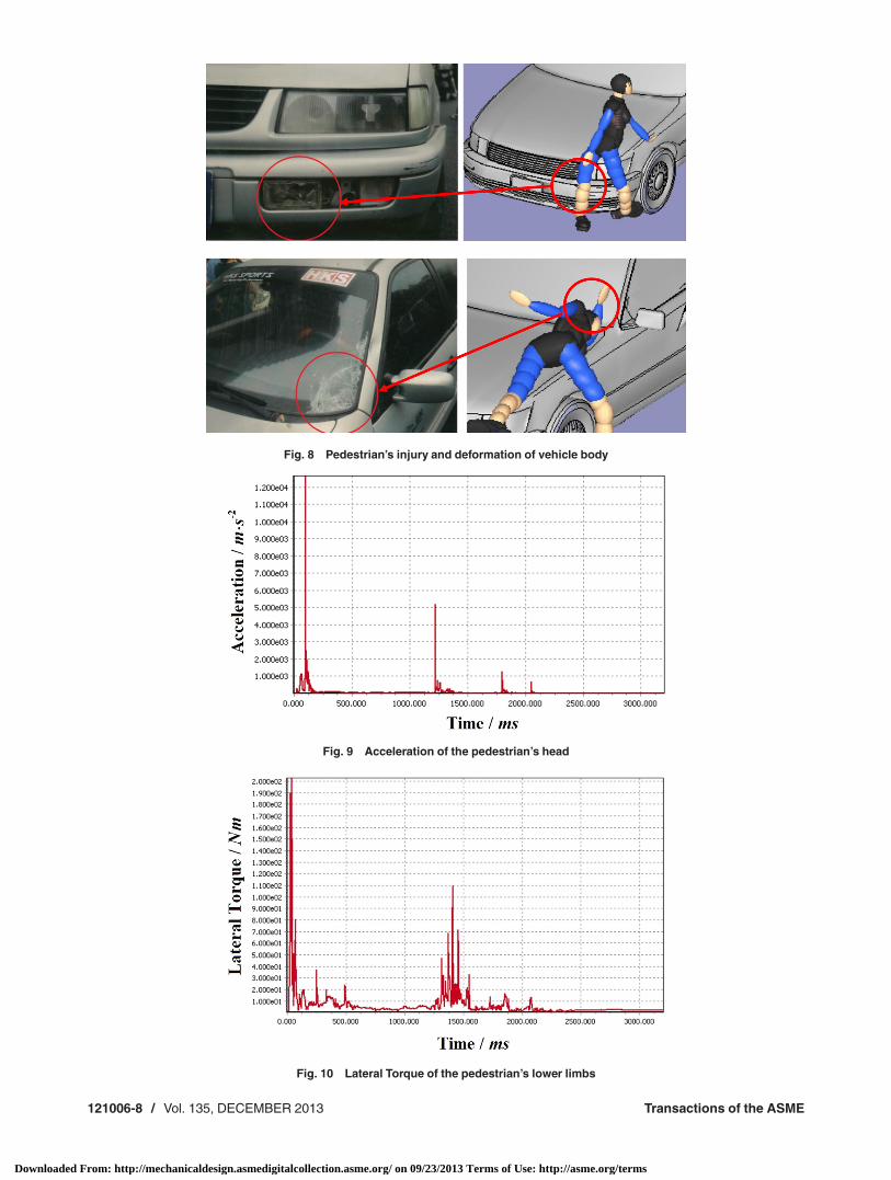
Fig. 8 Pedestrian’s injury and deformation of vehicle body

Fig. 10 Lateral Torque of the pedestrian’s lower limbs

Fig. 9 Acceleration of the pedestrian’s head

121006-8 / Vol. 135, DECEMBER 2013 Transactions of the ASME

Downloaded From: http://mechanicaldesign.asmedigitalcollection.asme.org/ on 09/23/2013 Terms of Use: http://asme.org/terms

4 times, the first two strikes being the most severe. The head hitthe windscreen and then the ground at two specific moments. Inaddition to the two fatal injuries on the head, we also investigatedthe other two injuries, which were not severe. Simulation resultssuggested that the tibia and fibula fractures were caused by thestrike at the very beginning when the pedestrian was hit by thebumper. The lateral torque curve of the pedestrian’s lower limbsis plotted in Fig. 10. This is also compatible with the forensicexamination.

6 Conclusions

Uncertainties exist in both parameters and model structures inalmost all the inverse simulations. Considering uncertainties ininverse simulation will increase the confidence of the inverse sim-ulation results. This work employs the maximum probability den-sity function to predict unknown model input variables, as well asthe realizations of random input variables whose prior joint proba-bility density functions are known, given that the simulation out-put variables are observed. The proposed probabilistic inversesimulation method is implemented by an optimization processwhere the joint probability density of the random input variablesis maximized while the constraints of the direct simulation equa-tions are maintained. The application of the proposed method in avehicle accident reconstruction indicates the effectiveness of themethod.

Using optimization to maximize the probability density, theproposed method can produce a unique solution to an inverse sim-ulation problem. The solution may not contain the true values fora given vehicle accident, and there might be multiple solutionsthat realize the given vehicle accident (or a given set of simulationoutput variables). But we have the highest confidence on the solu-tion from the proposed method because it produces the highestprobability density. To obtain multiple solutions, we may resort toan alternative method that uses conditional probabilities. Forexample, for the coefficient of friction in the application of thiswork, we could identify its probability density on conditional ofthe observed accident consequences, and we could also obtain itsconditional mean, variance, and other characteristics. This waywe will be able to obtain a family of solutions to a given set ofsimulation results. Our future work will test this alternativemethod and compare it with the present method.

Acknowledgement

We gratefully acknowledge the Institute of Forensic Science ofthe Ministry of the Justice of China and the Traffic Police Brigadeof Shanghai Municipal Public Security Bureau for collecting thereal-world data. The first author would like to acknowledge thesupport from the China Scholarship Council for his stay at theMissouri University of Science and Technology as a VisitingScholar and the support from the National Natural Science Foun-dation of China under Grant Nos. 50705058 and 60970049. Thelast two authors would like to thank the support from the NationalScience Foundation through Grant No. CMMI 1234855 and theIntelligent Systems Center (ISC) at the Missouri University ofScience and Technology.

References[1] Pontonnier, C., and Dumont, G., 2009, “Inverse Dynamics Method Using Opti-

mization Techniques for the Estimation of Muscles Forces Involved in theElbow Motion,” Int. J. Interact. Des. Manuf., 3(4), pp. 227–236.

[2] Tsai, M. S., and Yuan, W. H., 2010, “Inverse Dynamics Analysis for a 3-PrsParallel Mechanism Based on a Special Decomposition of the Reaction Forces,”Mech. Mach. Theory, 45(11), pp. 1491–1508.

[3] Paul, R. P., 1981, Robot Manipulators: Mathematics, Programming, and Con-trol: The Computer Control of Robot Manipulators, The MIT Press, ArtificialIntelligence Series, Cambridge, MA.

[4] Happee, R., 1994, “Inverse Dynamic Optimization Including Muscular Dynam-ics, a New Simulation Method Applied to Goal Directed Movements,” J. Bio-mech., 27(7), pp. 953–960.

[5] Blajer, W., and Czaplicki, A., 2001, “Modeling and Inverse Simulation of Som-ersaults on the Trampoline,” J. Biomech., 34(12), pp. 1619–1629.

[6] Crolet, J. M., Aoubiza, B., and Meunier, A., 1993, “Compact Bone:Numerical Simulation of Mechanical Characteristics,” J. Biomech., 26(6), pp.677–687.

[7] Blajer, W., Dziewiecki, K., and Mazur, Z., 2007, “Multibody Modeling ofHuman Body for the Inverse Dynamics Analysis of Sagittal Plane Movements,”Multibody Syst. Dyn., 18(2), pp. 217–232.

[8] Lu, L., 2007, “Inverse Modelling and Inverse Simulation for System Engineer-ing and Control Applications,” Ph.D. thesis, Faculty of Engineering, Universityof Glasgow, Scotland, UK.

[9] Murray-Smith, D. J., 2011, “Feedback Methods for Inverse Simulation ofDynamic Models for Engineering Systems Applications,” Math. Comput. Mod-ell. Dyn. Syst., 17(5), pp. 515–541.

[10] Blajer W., G. J., Krawczyk M., 2001, “Prediction of the Dynamic Characteris-tics and Control of Aircraft in Prescribed Trajectory Flight,” J. Theor. Appl.Mech., 39(1), pp. 79–103.

[11] Celi, R., 2000, “Optimization-Based Inverse Simulation of a Helicopter SlalomManeuver,” J. Guid. Control Dyn., 23(2), pp. 289–297.

[12] €Ostr€om, J., 2007, Enhanced Inverse Flight Simulation for a Fatigue Life Man-agement System, Hilton Head, SC, Vol. 1, pp. 60–68.

[13] Doyle, S. A., and Thomson, D. G., 2000, “Modification of a Helicopter InverseSimulation to Include an Enhanced Rotor Model,” J. Aircr., 37(3), pp. 536–538.

[14] De Divitiis, N., 1999, “Inverse Simulation of Aeroassisted Orbit Plane Changeof a Spacecraft,” J. Spacecr. Rockets, 36(6), pp. 882–889.

[15] Gu, X., Renaud, J. E., Batill, S. M., Brach, R. M., Budhiraja, A. S., 2000,“Worst Case Propagated Uncertainty of Multidisciplinary Systems in RobustDesign Optimization” Struct. Multidiscip. Optim., 20(3), pp. 190–213.

[16] Chen, W., Jin, R., and Sudjianto, A., 2005, “Analytical Variance-Based GlobalSensitivity Analysis in Simulation-Based Design under Uncertainty,” Trans.ASME J. Mech. Des., 127(5), pp. 875–886.

[17] Oberkampf, W. L., Deland, S. M., Rutherford, B. M., Diegert, K. V., and Alvin,K. F., 2002, “Error and Uncertainty in Modeling and Simulation,” Reliab. Eng.Syst. Saf., 75(3), pp. 333–357.

[18] Zhang, X. Y., Jin, X. L., Qi, W. G., and Guo, Y. Z., 2008, “Vehicle Crash Acci-dent Reconstruction Based on the Analysis 3D Deformation of the Auto-Body,”Adv. Eng. Software, 39(6), pp. 459–465.

[19] Xianghai, C., Xianlong, J., Xiaoyun, Z., and Xinyi, H., 2011, “The Applicationfor Skull Injury in Vehicle-Pedestrian Accident,” Int. J. Crashworthiness, 16(1),pp. 11–24.

[20] Lei, G., Xian-Long, J., Xiao-Yun, Z., Jie, S., Yi-Jiu, C., and Jian-Guo, C., 2008,“Study of Injuries Combining Computer Simulation in Motorcycle-Car Colli-sion Accidents,” Forensic Sci. Int., 177(2–3), pp. 90–96.

[21] Kokkolaras, M., Mourelatos, Z. P., and Papalambros, P. Y., 2006, “DesignOptimization of Hierarchically Decomposed Multilevel Systems underUncertainty,” ASME J. Mech. Des., 128(2), pp. 503–508.

[22] Zou, T., Cai, M., Du, R., and Liu, J., “Analyzing the Uncertainty of SimulationResults in Accident Reconstruction with Response Surface Methodology,” For-ensic Sci. Int., 216, pp. 49–60.

[23] Wach, W., and Unarski, J., 2007, “Uncertainty of Calculation Results in Vehi-cle Collision Analysis,” Forensic Sci. Int., 167(2–3), pp. 181–188.

[24] Du, X., 2012, “A Reliability Approach to Inverse Simulation underUncertainty,” The ASME 2012 International Design Engineering TechnicalConferences (IDETC) and Computers and Information in Engineering Confer-ence (CIE), ASME, Chicago.

[25] Chen, W., Baghdasaryan, L., Buranathiti, T., and Cao, J., 2004, “Model Valida-tion Via Uncertainty Propagation and Data Transformations,” AIAA J., 42(7),pp. 1406–1415.

[26] Liu, Y., Chen, W., Arendt, P., and Huang, H. Z., 2011, “Toward a Better Under-standing of Model Validation Metrics,” ASME J. Mech. Des., 133(7), p.071005.

[27] Youn, B. D., Jung, B. C., Xi, Z., Kim, S. B., and Lee, W. R., 2011, “A Hierarch-ical Framework for Statistical Model Calibration in Engineering Product Devel-opment,” Comput. Methods Appl. Mech. Eng., 200(13–16), pp. 1421–1431.

[28] Chen, W., Xiong, Y., Tsui, K. L., and Wang, S., 2008, “A Design-Driven Vali-dation Approach Using Bayesian Prediction Models,” Trans. ASME J. Mech.Des., 130(2), p. 021101.

[29] Chen, W., Yin, X., Lee, S., and Liu, W. K., 2010, “A Multiscale Design Meth-odology for Hierarchical Systems With Random Field Uncertainty,” Trans.ASME J. Mech. Des., 132(4), pp. 0410061–04100611.

[30] Drignei, D., Mourelatos, Z., Kokkolaras, M., Li, J., and Koscik, G., 2011, “AVariable-Size Local Domain Approach to Computer Model Validation inDesign Optimization,” SAE Int. J. Mater. Manuf., 4(1), pp. 421–429.

[31] Ferson, S., and Oberkampf, W. L., 2009, “Validation of Imprecise ProbabilityModels,” Int. J. Reliab. Saf., 3(1–3), pp. 3–22.

[32] Ferson, S., Oberkampf, W. L., and Ginzburg, L., 2008, “Model Validation andPredictive Capability for the Thermal Challenge Problem,” Comput. MethodsAppl. Mech. Eng., 197(29–32), pp. 2408–2430.

[33] Xiong, Y., Chen, W., and Tsui, K. L., 2008, “A New Variable-Fidelity Optimi-zation Framework Based on Model Fusion and Objective-Oriented SequentialSampling,” ASME J. Mech. Des., 130(11), pp. 1114011–1114019.

[34] Xi, Z., Youn, B. D., and Hu, C., 2010, “Random Field Characterization Consid-ering Statistical Dependence for Probability Analysis and Design,” ASMEJ. Mech. Des., 132(10), p. 101008

Journal of Mechanical Design DECEMBER 2013, Vol. 135 / 121006-9

Downloaded From: http://mechanicaldesign.asmedigitalcollection.asme.org/ on 09/23/2013 Terms of Use: http://asme.org/terms

[35] Goda, K., 2010, “Statistical Modeling of Joint Probability Distribution UsingCopula: Application to Peak and Permanent Displacement Seismic Demands,”Struct. Saf., 32(2), pp. 112–123.

[36] Noh, Y., Choi, K. K., and Du, L., 2009, “Reliability-Based Design Optimizationof Problems with Correlated Input Variables Using a Gaussian Copula,” Struct.Multidiscip. Optim., 38(1), pp. 1–16.

[37] Choi, S. K., Grandhi, R. V., and Canfield, R. A., 2007, Reliability-Based Struc-tural Design, Springer, New York.

[38] Eldred, M. S., and Burkardt, J., 2009, “Comparison of Non-Intrusive PolynomialChaos and Stochastic Collocation Methods for Uncertainty Quantification,”

47th AIAA Aerospace Sciences Meeting including The New Horizons Forum andAerospace Exposition, Orlando, FL, January 2009, Paper No. 2009-0976.

[39] Sudret, B., 2008, “Global Sensitivity Analysis Using Polynomial ChaosExpansions,” Reliab. Eng. Syst. Saf., 93(7), pp. 964–979.

[40] Chen, W., Tsui, K.-L., Allen, J. K., and Mistree, F., 1995, “Integration ofthe Response Surface Methodology With the Compromise DecisionSupport Problem in Developing a General Robust Design Procedure,”Proceedings of the 1995 ASME Design Engineering Technical Conference,September 17–20, Boston, MA, ASME, Des. Eng. Div. 82(1), 485–492(1995).

121006-10 / Vol. 135, DECEMBER 2013 Transactions of the ASME

Downloaded From: http://mechanicaldesign.asmedigitalcollection.asme.org/ on 09/23/2013 Terms of Use: http://asme.org/terms