xiv conference for young researchers
TRANSCRIPT

13-15. APRIL 2016, PLEVEN, BULGARIA
ISS
N 2
535-0
196 (
Pri
nt)
, IS
SN
2535-0
20X
(O
nline)
YE
AR
4, V
OLU
ME
1(4
)
XIV CONFERENCE FOR YOUNG RESEARCHERS
10-13.03.2021, BOROVETS, BULGARIA
XVIII INTERNATIONAL SCIENTIFIC CONGRESS
MACHINES. MATERIALS TECHNOLOGIES.
SCIENTIFIC TECHNICAL UNIONOF MECHANICAL ENGINEERING
BULGARIA

XVIII INTERNATIONAL SCIENTIFIC CONGRESS
MACHINES. TECHNOLOGIES. MATERIALS.
XIV INTERNATIONAL CONFERENCE
FOR YOUNG RESEARCHERS
TTEECCHHNNIICCAALL SSCCIIEENNCCEESS..
IINNDDUUSSTTRRIIAALL MMAANNAAGGEEMMEENNTT 10 – 13.03.2021 BOROVETS, BULGARIA
INTERNATIONAL EDITORIAL BOARD CHAIRMAN:
Prof. Dr. Econ. Cyril Angelov (Bulgaria)
MEMBERS: Anatoly Magidenko, Prof. (Latvia)
Dzhavit Kuramshin, Assoc. Prof. (Russia)
Elizabeta Hristovska, Prof. (North Macedonia)
Emil Trifonov, Assoc. Prof. (Bulgaria)
Emilia Abadjieva, Assoc. Prof. (Japan)
Irena Macherinskine, Prof. (Lithuania)
Ivan Dimitrov, Prof. (Bulgaria)
Ivan Kuric, Prof. (Slovakia)
Konstantins Didenko, Prof. (Latvia)
Laura Bakalli, Prof. (Romania)
Loretta Parashkevova, Prof. (Bulgaria)
Lyubomir Dimitrov, Prof. (Bulgaria)
Maryna Chaikovska, Assoc. Prof. (Ukraine)
Matilda Alexandrova, Prof. (Bulgaria)
Nikolay Dolgov, Assoc. Prof. (Ukraine)
Nikolay Hinov, Prof. (Bulgaria)
Pancho Tomov, Prof. (Bulgaria)
Rima Tamosiunine, Prof. (Lithuania)
Sergei Voytko, Prof. (Ukraine)
Sergey Lezhnev, Assoc. Prof. (Kazakhstan)
Valeriy Sorokin, Assoc. Prof. (Belarus)
Vedran Mrzljak, Assoc. Prof. (Croatia)
Yvonne Novak-Marchinchin, Prof. (Slovakia)
PUBLISHER:
THE SCIENTIFIC TECHNICAL UNION
OF MECHANICAL ENGINEERING “INDUSTRY 4.0”
ISSN 2535-0196 (Print), ISSN 2535-020X (Online)
Year IV Volume 1(4) MARCH 2021

C O N T E N T S
Energy and exergy losses analysis of back-pressure steam turbine from CHP plant Mrzljak Vedran, Prpić-Oršić Jasna, Poljak Igor, Lorencin Ivan ..................................................................................... 3
Recycle rechargeable lithium - ion batteries Stela Todorova, Mladen Proykov .................................................................................................................................... 7
Мathematical analysis of an electrical circuit Stela Todorova, Mladen Proykov .................................................................................................................................... 9
The use of encapsulated sodium ferrate in wastewater treatment in the production of animal feed Altynbayeva Gulnara, Kadnikova Olga ......................................................................................................................... 11
Generation of test sequences with a given switching activity Mikalai Shauchenka ...................................................................................................................................................... 14
Investigation of solders surface tension in temperature range from melting point up to 673К Plamen V. Petkov, Dimitar Lyutov, Hristo Iliev ........................................................................................................... 18
Open innovation – potential, constraints and prospects Borislava Galabova ........................................................................................................................................................ 22
Application of different color systems to determine the visual characteristics of beer Христина Андреева, Владимира Ганчовска, Радослава Габрова ............................................................................ 26
Application of computer vision to determine the size and distribution of additives in cakes Христина Андреева, Владимира Ганчовска .............................................................................................................. 29

Energy and exergy losses analysis of back-pressure steam turbine from chp plant
Mrzljak Vedran1, Prpić-Oršić Jasna1, Poljak Igor2, PhD. Lorencin Ivan1 1Faculty of Engineering, University of Rijeka, Vukovarska 58, 51000 Rijeka, Croatia
2Department of maritime sciences, University of Zadar, Mihovila Pavlinovića 1, 23000 Zadar, Croatia
E-mail: [email protected], [email protected], [email protected], [email protected]
Abstract: In this paper is analyzed back-pressure steam turbine which operates in CHP (Combined Heat and Power) plant from the aspect of
energy and exergy losses. Produced turbine power, used for electricity generator drive equals 62548.77 kW, while the turbine mechanical loss is 1934.50 kW. Exergy analysis of the turbine shows that cumulative exergy loss is composed of two losses - mechanical loss and steam
exergy loss. Steam exergy loss is additional loss which takes into account the state of the ambient in which turbine operates (unlike energy analysis which is independent of the ambient state). Change in the ambient temperature resulted with a change in turbine exergy efficiency
and exergy loss. Ambient temperature change for 10 °C resulted with change in turbine exergy efficiency for less than 0.5 % on average,
while the change in the turbine exergy loss (for the same temperature change) equals 266.21 kW on average.KEYWORDS: BACK-PRESSURE STEAM TURBINE, ENERGY LOSS, EXERGY LOSS, CHP PLANT
1. Introduction
Steam turbines are nowadays the basic power producers whichdrive electricity generators and produce electric power [1, 2]. The
majority of such steam turbines (for electricity generator drive) are condensation type, which mean that steam after expansion through
the turbine has pressure lower than atmospheric pressure – such steam is delivered to a steam condenser (or more of them) [3, 4].
Some steam turbines which operate in steam power plants are also used for electricity generators drive, but are of back-pressure
type (steam after expansion in the turbine has pressure above the
atmospheric pressure and is used for heating of any heat consumer [5]). Such steam turbine is analyzed in this paper.
Based on measured steam operating parameters from the literature [6] it is performed energy and exergy analysis of back-
pressure steam turbine. Energy analysis involved mechanical loss which occurs in the turbine cylinder. It is investigated energy and
exergy flow streams throughout analyzed steam turbine and it is compared energy and exergy losses. Cumulative exergy loss of the
analyzed turbine contains additional steam loss which cannot be
obtained through energy analysis of the same turbine. The variation of the ambient temperature is also performed – to investigate
turbine operating parameters, exergy loss and exergy efficiency at different ambient conditions.
2. Description of the analyzed back-pressure steam
turbine from CHP plant
Back-pressure steam turbine which operates in CHP plant [6] is analyzed in this paper from the energy and exergy aspect. General
operating scheme of the analyzed turbine is presented in Fig. 1. Produced power from the analyzed steam turbine is used for
electricity generator drive. In the energy analysis, mechanical loss which occurs into the turbine is taken into account. In this case,
steam turbine drive electricity generator directly (without the gearbox usage). If the steam turbine drives any other power
consumer through the gearbox, than the mechanical loss of the
gearbox also must be taken into account when calculating power amount distributed to power consumer.
Complete energy and exergy analysis of back-pressure steam turbine is based on three turbine operating points presented in Fig 1.
– the first operating point is turbine inlet, the second is steamextraction and last third operating point is turbine outlet. As the
exergy analysis of any component in the steam power plant isdependable on the conditions of the ambient (the ambient
temperature and pressure) [7, 8] this analysis also includes variation
of the ambient temperature in order to obtain turbine exergy lossand exergy efficiency at different ambient conditions.
Fig. 1. Scheme and operating points of the analyzed back-pressure
steam turbine from CHP plant
3. Equations for energy and exergy analysis
3.1. General equations
For any analyzed control volume or a system in which mass flow rate leakage does not occur is valid a following mass flow rate
balance [9]:
OUTIN mm , (1)
where: IN = inlet (input), OUT = outlet (output), m = fluid mass
flow rate (kg/s). The first law of thermodynamics gives a definition
of energy analysis [10], which is completely independent of the
ambient conditions in which analyzed control volume or a system operates [11]. Basic energy balance for a control volume or a
system in steady state while disregarding potential and kinetic energy, according to [12, 13] is:
PhmQhm OUTOUTININ , (2)
where: h = fluid specific enthalpy (kJ/kg), Q = heat transfer
(kW), P = produced power (kW). Energy power of any fluid flow (n), according to [14] is defined as:
nnnEN, hmE , (3)
where: nEN,E = energy power of fluid flow (kW), n = index for
observed operating point (fluid flow). Unlike energy analysis, exergy analysis of control volume or a system is defined by the
second law of thermodynamics [15]. Exergy analysis is based on
the ambient conditions in which control volume or a system operates [16]. The main exergy balance equation, according to [17,
18] can be written as:
DEX,OUTOUTheatININ EPmXm , (4)
where: DEX,E
= exergy destruction = exergy loss (kW). In Eq. 4,
heatX is the exergy transfer by heat (kW) at the temperature T (K)
which is defined, according to [19, 20] as:
TECHNICAL SCIENCES. INDUSTRIAL MANAGEMENT. 2021
3

QT
TX )1( 0
heat , (5)
where: 0 = index of the ambient condition. The last undefined
parameter from Eq. 4 is specific exergy of the fluid stream ( ),
which definition can be found in [21]:
)()( 000 ssThh , (6)
where: s = fluid specific entropy (kJ/kg·K). Similar to energypower of fluid flow, exergy power of any fluid flow (n) can be
defined by following equation [22]:
nnnEX, mE , (7)
where: nEX,E = exergy power of fluid flow (kW). For any control
volume or a system, general definition of exergy efficiency (EX ),
according to [23] is:
inputExergy
outputExergyEX . (8)
3.2. Energy and exergy analysis of back-pressure steam
turbine from CHP plant
All the equations for the energy and exergy analysis of back-pressure steam turbine from CHP plant in this section will be based
on turbine operating points from Fig. 1.
3.2.1. Energy analysis
Turbine power, without taking into account the mechanical loss,
is calculated from steam expansion throughout the turbine as:
)()()( 3221211T hhmmhhmP , (9)
where: TP = turbine power without mechanical loss (kW).
Turbine real power, with taking into account the mechanical loss is:
MECHTMECH3221211RE )()()( PhhmmhhmP , (10)
where: REP = turbine real developed power with mechanical loss
(kW), MECH = turbine mechanical efficiency (%). In the analysis
is assumed that mechanical efficiency of the observed back-pressure steam turbine is equal to 97 %. From Eq. 9 and Eq. 10, analyzed
turbine mechanical loss is:
)1( MECHTMECHTTRETMECH PPPPPP , (11)
where: MECHP = turbine mechanical loss (kW). Energy power of
fluid (steam) flow in each operating point of the analyzed turbine (Fig. 1) is calculated by using Eq. 3.
3.2.2. Exergy analysis
Cumulative exergy loss (cumulative exergy destruction) of the analyzed turbine is:
MECHTEX,3EX,2EX,1REEX,3EX,2EX,1CUMD,EX, PPEEEPEEEE ,
(12)
where: CUMD,EX,E = turbine cumulative exergy loss (kW).
Cumulative exergy loss of the turbine (CUMD,EX,E ) can be divided
on two different losses - the first is a steam exergy loss (steamD,EX,E )
and the second is mechanical loss (MECHP ) defined by Eq. 11.
Therefore, steam exergy loss is:
TEX,3EX,2EX,1steamD,EX, PEEEE , (13)
where: steamD,EX,E = steam exergy loss (kW). Analyzed back-
pressure steam turbine exergy efficiency is:
EX,3EX,2EX,1
MECHT
EX,3EX,2EX,1
REEX
EEE
P
EEE
P
. (14)
Exergy power of fluid (steam) flow in each operating point of the analyzed turbine (Fig. 1) is calculated by using Eq. 7.
4. Steam operating parameters of the analyzed back-
pressure turbine
Steam operating parameters (pressure, temperature and mass flow
rate) in each operating point of the analyzed back-pressure turbine
(Fig. 1) were found in [6] and presented in Table 1. In all operating points steam is superheated.
Table 1. Steam operating parameters in each operating point of
analyzed back-pressure turbine [6]
Operating point*
Pressure (bar)
Temperature (°C)
Mass flow rate (kg/s)
1 84.0 500.0 103.7
2 11.0 232.5 15.6
3 3.5 147.0 88.1
* Operating points refer to Fig. 1.
To perform complete energy and exergy analysis along with
calculation of losses, steam operating parameters from Table 1 is
used for calculation of specific enthalpy, specific entropy and specific exergy again in each operating point of the observed
turbine. Those operating parameters were calculated by using NIST-REFPROP 9.0 software [24] and presented in Table 2.
Table 2. Steam specific enthalpy, specific entropy and specific
exergy in each operating point of analyzed turbine
Operating point*
Specific enthalpy
(kJ/kg)
Specific entropy
(kJ/kg·K)
Specific exergy
(kJ/kg)
1 3394.7 6.70 1401.80
2 2899.8 6.80 876.91
3 2750.4 6.99 672.54
* Operating points refer to Fig. 1.
Steam specific exergies in Table 2 are calculated for the base ambient state which is in this paper selected as: the ambient
pressure = 1 bar, the ambient temperature = 25 °C = 298 K.
5. The results of performed analysis and discussion
5.1. Back-pressure steam turbine energy and exergy losses at
the base ambient state
In Fig. 2 are presented energy flow streams throughout the analyzed steam turbine (steam energy streams at turbine inlet, outlet
and at turbine extraction). While neglecting steam mass flow rates lost on the turbine front and rear gland seals, cumulative produced
power of the analyzed turbine (power without taking into account the mechanical loss) is equal to the steam energy flow stream at the
turbine inlet lowered for steam energy flow streams at turbine outlet
and at turbine extraction. A power which will be used for any power consumer drive (in
this case electricity generator drive) is lower (in comparison with power without taking into account the mechanical loss) for
mechanical loss into the analyzed turbine. The calculation of this power is ensured with Eq. 10 (power with taking into account the
mechanical loss). According to steam operating parameters of the analyzed back-pressure turbine (Table 1 and Table 2), mechanical
loss is equal to 1934.50 kW, while power for the electricity
generator drive will be equal to 62548.77 kW, Fig. 2. It should be noted that if the power consumer is driven by the analyzed turbine
indirectly (by using gearbox) mechanical power delivered to such power consumer should be additionally lowered for mechanical loss
in the gearbox.
TECHNICAL SCIENCES. INDUSTRIAL MANAGEMENT. 2021
4

Fig. 2. Energy flow streams of the analyzed back-pressure steam
turbine
Exergy flow streams and exergy loss throughout the analyzed
back-pressure turbine at the base ambient state are presented in Fig. 3. First of all, it should be noted that steam exergy streams (at
turbine inlet, outlet and at turbine extraction) are much lower when
compared to the same steam energy streams (Fig. 2). Analyzed turbine power produced, mechanical loss and power
used for electricity generator drive are the same as in energy analysis (Fig. 2). As the exergy analysis takes into account the
conditions of the ambient in which turbine operates, a cumulative turbine exergy loss which amount 9887.32 kW can be divided in
two parts – the first is mechanical loss and the second is a steam exergy loss which is for the analyzed turbine equal to 7952.82 kW,
Fig. 3. Like in energy analysis, in the turbine exergy analysis are
also neglected steam mass flow rates lost through front and rear gland seals.
The analyzed back-pressure steam turbine is a good example that exergy analysis (in comparison with energy analysis) involves
additional loss related to the ambient conditions.
Fig. 3. Exergy flow streams of the analyzed back-pressure steam
turbine (the base ambient state)
5.2. Back-pressure steam turbine exergy loss during the
ambient temperature change
The analyzed back-pressure steam turbine has three operating
points – the first is turbine inlet, the second is turbine extraction and the third is turbine outlet, Fig. 1. Exergy flow streams (steam exergy
streams) in each turbine operating point, during the change in the ambient temperature are presented in Fig. 4. From Fig. 4 can clearly
be seen that the change in ambient temperature significantly influenced steam exergy streams of the analyzed turbine – increase
in the ambient temperature decreases each steam exergy stream in
all operating points. The ambient temperature in which analyzed turbine operates is
varied from 5 °C to 55 °C. In such ambient temperature range, steam exergy stream at the turbine inlet decreases the most during
the ambient temperature increase, for 32499.58 kW (from 158806.18 kW at the ambient temperature of 5 °C to 126306.6 kW
at the ambient temperature of 55 °C), while the lowest decrease in
the steam exergy stream during the ambient temperature increase can be observed for steam extraction (Operating point 2), Fig. 4.
Fig. 4. Exergy flow streams (steam exergy streams) in each
operating point of the analyzed back-pressure turbine during the ambient temperature change (according to Fig. 1)
Decrease in all analyzed turbine steam exergy streams during the increase in the ambient temperature resulted with an increase in
turbine cumulative exergy loss (from 9362.71 kW at the ambient temperature of 5 °C to 10693.75 kW at the ambient temperature of
55 °C), Fig. 5. It should be noted that in cumulative turbine exergy loss, mechanical loss remains the same at all observed ambient
temperatures, while steam exergy loss notably increases during the
increase in the ambient temperature. An increase in the ambient temperature simultaneously increases
analyzed turbine cumulative exergy loss and decreases turbine exergy efficiency, from 86.98 % at 5 °C to 85.40 % at 55 °C. It can
be concluded that an increase in the ambient temperature for 10 °C reduces analyzed back-pressure turbine exergy efficiency for less
than 0.5 % on average, so the analyzed turbine exergy efficiency is
not significantly influenced by the ambient temperature change. However, the ambient temperature change notably influenced
analyzed turbine cumulative exergy loss which increase for 266.21 kW on average for every increase in the ambient temperature in step
of 10 °C.
Fig. 5. Cumulative exergy loss and exergy efficiency of analyzed
steam turbine during the ambient temperature change
Further research and possible optimization of the observed steam turbine will be performed by the application of many artificial
intelligence methods and processes already developed and
implemented by our research team [25-30].
6. ConclusionsIn this paper is presented energy and exergy losses analysis of
back-pressure steam turbine from a CHP plant. Energy analysis
takes into account only mechanical loss (energy flows lost through front and rear gland seals are neglected). Exergy analysis is
performed for the selected base ambient state and then the ambient temperature is varied in order to obtain the change in turbine exergy
efficiency and loss. The major conclusions of this analysis are: - Analyzed back-pressure steam turbine, for the known steam
operating parameters and mechanical efficiency equal to 97 %, hasmechanical loss equal to 1934.50 kW and produced 62548.77 kW
of power used for electricity generator drive. Energy analysis of this
(and any other steam turbine) is always the same - it did not dependon the ambient conditions in which turbine operates.
TECHNICAL SCIENCES. INDUSTRIAL MANAGEMENT. 2021
5

- Exergy analysis shows that cumulative exergy loss of the analyzedturbine is composed of the sum of two losses - mechanical loss and
steam exergy loss. Therefore, exergy analysis takes into accountadditional loss related to the state of the ambient in which steam
turbine operates.- An increase in the ambient temperature resulted with a decrease in
all steam exergy streams of the analyzed turbine. The most notable
change in steam exergy streams during the ambient temperaturechange is observed for the steam stream at the turbine inlet.
- An increase in the ambient temperature reduces turbine exergyefficiency (and vice versa) but the change is small. Notable change
during the ambient temperature change is observed in the turbineexergy loss. An increase in the ambient temperature for 10 °C
resulted with an average decrease of analyzed turbine exergyefficiency for less than 0.5 % and simultaneously with an average
increase of turbine exergy loss for 266.21 kW.
7. AcknowledgmentThis research has been supported by the Croatian Science
Foundation under the project IP-2018-01-3739, CEEPUS network CIII-HR-0108, European Regional Development Fund under the
grant KK.01.1.1.01.0009 (DATACROSS), project CEKOM under the grant KK.01.2.2.03.0004, CEI project “COVIDAi” (305.6019-
20), University of Rijeka scientific grant uniri-tehnic-18-275-1447 and University of Rijeka scientific grant uniri-tehnic-18-18-1146.
8. References[1] Wilding, P. R., Murray, N. R., & Memmott, M. J. (2020). The
use of multi-objective optimization to improve the design process of nuclear power plant systems. Annals of Nuclear Energy, 137,107079. (doi:10.1016/j.anucene.2019.107079)
[2] Lorencin, I., Anđelić, N., Mrzljak, V., & Car, Z. (2019). Genetic Algorithm Approach to Design of Multi-Layer Perceptron for Combined Cycle Power Plant Electrical Power Output
Estimation. Energies, 12(22), 4352. (doi:10.3390/en12224352) [3] Pattanayak, L., Padhi, B. N., & Kodamasingh, B. (2019). Thermal
performance assessment of steam surface condenser. Case
Studies in Thermal Engineering, 14, 100484. (doi:10.1016/j.csite.2019.100484)
[4] Škopac, L., Medica-Viola, V., & Mrzljak, V. (2020). SelectionMaps of Explicit Colebrook Approximations according toCalculation Time and Precision. Heat Transfer Engineering,
1-15. (doi:10.1080/01457632.2020.1744248) [5] Kostyuk, A., & Frolov, V. (Eds.). (1988). Steam and gas
turbines. Mir Pub..
[6] Holmberg, H., Tuomaala, M., Haikonen, T., & Ahtila, P. (2012). Allocation of fuel costs and CO2-emissions to heat and power in an industrial CHP plant: Case integrated pulp and paper mill.
Appl. En., 93, 614-623.(doi: 10.1016/j.apenergy.2011.11.040) [7] Zueco, J., López-Asensio, D., Fernández, F. J., & López-
González, L. M. (2020). Exergy analysis of a steam-turbine power plant using thermocombustion. Appl. Therm. Eng., 180,115812. (doi: 10.1016/j.applthermaleng.2020.115812)
[8] Baressi Šegota, S., Lorencin, I., Anđelić, N., Mrzljak, V., & Car, Z. (2020). Improvement of Marine Steam Turbine ConventionalExergy Analysis by Neural Network Application. Journal of
Marine Sci. and Eng., 8(11), 884. (doi:10.3390/jmse8110884) [9] Lorencin, I., Anđelić, N., Mrzljak, V., & Car, Z. (2019). Exergy
analysis of marine steam turbine labyrinth (gland) seals.
Pomorstvo, 33(1), 76-83. (doi:10.31217/p.33.1.8) [10]Kanoğlu, M., Çengel, Y. A. & Dincer, I. (2012). Efficiency
Evaluation of Energy Systems. Springer.(doi:10.1007/978-1-4614-2242-6)
[11]Medica-Viola, V., Baressi Šegota, S., Mrzljak, V., & Štifanić, D.
(2020). Comparison of conventional and heat balance based energy analyses of steam turbine. Pomorstvo, 34(1), 74-85. (doi:10.31217/p.34.1.9)
[12]Ahmadi, G. R., & Toghraie, D. (2016). Energy and exergy analysis of Montazeri steam power plant in Iran. Renewable and Sust. Energy Rev., 56, 454-463. (doi:10.1016/j.rser.2015.11.074)
[13]Mrzljak, V., & Poljak, I. (2019). Energy Analysis of Main Propulsion Steam Turbine from Conventional LNG Carrier at
Three Different Loads. NAŠE MORE, 66(1), 10-18. (doi:10.17818/NM/2019/1.2)
[14]Aljundi, I. H. (2009). Energy and exergy analysis of a steam power plant in Jordan. Applied Thermal Eng., 29(2-3), 324-328. (doi:10.1016/j.applthermaleng.2008.02.029)
[15]Szargut, J. (2005). Exergy method: technical and ecological applications (Vol. 18). WIT press.
[16]Medica-Viola, V., Mrzljak, V., Anđelić, N., & Jelić, M. (2020).
Analysis of Low-Power Steam Turbine With One Extraction for Marine Applications. NAŠE MORE, 67(2), 87-95.
(doi:10.17818/NM/2020/2.1) [17]Baldi, F., Ahlgren, F., Nguyen, T. V., Thern, M., & Andersson,
K. (2018). Energy and exergy analysis of a cruise ship. Energies,
11(10), 2508. (doi:10.3390/en11102508) [18]Mrzljak, V., Blecich, P., Anđelić, N., & Lorencin, I. (2019).
Energy and Exergy Analyses of Forced Draft Fan for Marine
Steam Propulsion System during Load Change. Journal ofMarine Sci. and Eng., 7(11), 381. (doi:10.3390/jmse7110381)
[19]Koroglu, T., & Sogut, O. S. (2018). Conventional and advanced
exergy analyses of a marine steam power plant. Energy, 163, 392-403. (doi:10.1016/j.energy.2018.08.119)
[20]Mrzljak, V., Poljak, I., & Prpić-Oršić, J. (2019). Exergy analysis of the main propulsion steam turbine from marine propulsion plant. Brodogradnja, 70(1), 59-77. (doi:10.21278/brod70105)
[21]Tan, H., Shan, S., Nie, Y., & Zhao, Q. (2018). A new boil-off gas re-liquefaction system for LNG carriers based on dual mixed refrigerant cycle. Cryogenics, 92, 84-92.
(doi:10.1016/j.cryogenics.2018.04.009) [22]Mrzljak, V., Senčić, T., & Ţarković, B. (2018). Turbogenerator
steam turbine variation in developed power: Analysis of exergy
efficiency and exergy destruction change. Modelling andSimulation in Engineering, 2018. (doi:10.1155/2018/2945325)
[23]Mrzljak, V., Poljak, I., & Medica-Viola, V. (2017). Dual fuelconsumption and efficiency of marine steam generators for the propulsion of LNG carrier. Applied Thermal Engineering, 119,
331-346. (doi:10.1016/j.applthermaleng.2017.03.078) [24]Lemmon, E. W., Huber, M. L., & McLinden, M. O. (2010). NIST
Standard Reference Database 23, Reference Fluid
Thermodynamic and Transport Properties (REFPROP), version 9.0, National Institute of Standards and Technology. R1234yf.fld file dated December, 22, 2010.
[25]Baressi Šegota, S., Lorencin, I., Ohkura, K., & Car, Z. (2019).On the Traveling Salesman Problem in Nautical Environments:
an Evolutionary Computing Approach to Optimization of Tourist Route Paths in Medulin, Croatia. Pomorski zbornik, 57(1), 71-87. (doi:10.18048/2019.57.05)
[26]Lorencin, I., Anđelić, N., Mrzljak, V., & Car, Z. (2019). Marine Objects Recognition Using Convolutional Neural Networks.NAŠE MORE, 66(3), 112-119. (doi:10.17818/NM/2019/3.3)
[27]Car, Z., Baressi Šegota, S., Anđelić, N., Lorencin, I., & Mrzljak, V. (2020). Modeling the Spread of COVID-19 Infection Using aMultilayer Perceptron. Computational and Mathematical
Methods in Medicine, 2020. (doi:10.1155/2020/5714714) [28]Lorencin, I., Anđelić, N., Mrzljak, V., & Car, Z. (2019).
Multilayer Perceptron approach to Condition-Based Maintenance of Marine CODLAG Propulsion System Components. Pomorstvo, 33(2), 181-190.
(doi:10.31217/p.33.2.8) [29]Baressi Šegota, S., Lorencin, I., Musulin, J., Štifanić, D., & Car,
Z. (2020). Frigate Speed Estimation Using CODLAG Propulsion
System Parameters and Multilayer Perceptron. NAŠE MORE, 67(2), 117-125. (doi:10.17818/NM/2020/2.4)
[30]Lorencin, I., Anđelić, N., Šegota, S. B., Musulin, J., Štifanić, D.,
Mrzljak, V., ... & Car, Z. Edge Detector-Based Hybrid Artificial Neural Network Models for Urinary Bladder Cancer Diagnosis.
In Enabling AI Applications in Data Science (pp. 225-245). Springer, Cham.
TECHNICAL SCIENCES. INDUSTRIAL MANAGEMENT. 2021
6

Recycle rechargeable lithium - ion batteries
Stela Todorova, Mladen Proykov
University “Prof. d-r Asen Zlatarov”, “Prof. Yakimov” bul, 8010 Burgas,, Bulgaria
Abstract: Milliards of dollars are set aside for preserving the life on planet Earth and help climate change. Unfortunately, the advances in
technology are incapable to help us sort out this vital problem, because the more advanced the technology nowadays is, more irresponsible
we become in taking care about consequences after the expiration date of it. It is not only the plastic pollution of ocean of our planet that
stops the formation of oxygen but also the irresponsible disposal of lithium-ion rechargeable batteries for smartphones, tablets, computers,
electric smart devices and vehicles that are no longer in use, create ionizing radiation and form a radioactive background that affects living
and non-living organisms inhabiting our planet. So, when the technology cannot help us, then perhaps the pure science would come to the
rescue of preserving ourselves. There are laboratory researches about recycling lithium-ion batteries and here where we are – we are going
to implement mathematics, algorithms, indexed arrays(vectors) for describing the benefit of manufacturing the recycling of lithium-ion
batteries.
Keywords: RECYCLING, BATTERY, ELECTRIC CAR, ELECTRICITY
1. Introduction
Bodies in nature are divided into three groups or categories:
1) Radioactive (RA) forms, which contain positive and negative
electricity, forming atomic bombardment, which, hitting the ether,
gives constant waves;
2) Forms that contain only positive electricity;
3) Forms that contain only negative electricity.
Based on categories 1), 2) and 3), Louis Turenne created
detectors for each one of 3 groups:
1. Normal radioactive detector;
2. Detector (minus) - (negative);
3. Detector (plus) - (positive);
Using these three detectors and applying his theory of wave
propagation, he was able to find out that all radioactive forms emit
constant waves and that the forms of the second and third groups,
placed under certain conditions, also emit waves, but they are not
constant, which he called pendulum /static/ waves.
Also, engineer Louis Turenne was able to graphically trace the
spectra of these static waves, when it is impossible to study the
spectrum of constant waves, which are excessively short, node to
node and practically represent continuous straight lines. [1]
Tesla and other scientists speculated that electric and magnetic
forces were actually streams of ether that is fixed in matter.
Materials are somehow "polarized" by "rubbing" as the ether passes
through them. Most substances maintain the flow indefinitely
because it does not make them work. It is enough for matter to
simply remain polarized in order to conduct the flow of the ether.
[2]
According to these theories it is possible to conclude:
Conclusion N 1: All radioactive bodies emit constant waves -
Wave that results from impacts on the ether, with a uniform
frequency, and as a result of mechanical, electrical, magnetic,
atomic or other bombardment. These waves are also known by the
radio as carriers.
Conclusion N 2: All other forms emit static waves, which the
detectors will encounter in the form of spheres or ellipsoids, which
are usually 4 groups, one after the other and are repeated in the 4
perpendicular directions in which the constant carrier wave
propagates. The wavelength of each group is L and consists of 4
ellipsoids. For the 4 groups in the direction of the carrier wave will
be L, 2L, 3L, 4L. The four concentric spheres or ellipses have wave
heights h, 2h, 3h, 4h, respectively. An abbreviated image of a static
wave can be represented by knowing the direction of the (+) or (-)
wave and the value of the first h and L.
Louis Turenne draws the following conclusion after many
experiments: mechanical or atomic shock waves follow the same
laws and create the same constant waves as those of mechanical
waves created by a metronome, whose length increases as the
frequency of shocks per minute decreases. Louis Turenne draws
another important conclusion that the waves that are measured
appear to be harmonic to the waves measured in μ.
On the other hand, in physics, the wavelengths of colors in μ are
set, as well as their frequencies in billions of kilocycles, the
wavelengths of which are given in Table 1. [1]
Table 1. Measuring scales. [1]
Measuring scales Value 1 Value 2 Value 3 Value 4
Colours Red Yellow Green Blue
Length in μ 0.64 0.56 0.52 0.48
Frequency in
billions of
kilocycles
380
520
580
640
2. Lithium-ion battery and principle of operation
Nowadays, the lithium-ion battery is one of the most popular
types of batteries in portable electronic devices - electric cars,
laptops, smartphones, tablets and other portable devices. The three
main functional components of a lithium-ion battery are the anode,
cathode and electrolyte, for the manufacture of which different
materials can be used. The most popular material for the anode is
graphite. [3]
Fig. 1 shows a three-dimensional image of the grid of the
cathode, where the atoms of the chemical elements are represented
as vertices of a polyhedron - 3-Dimensional figure, which are used
to make it, and the covalent bonds that exist between the chemical
elements are represented as sides of the polyhedron.
Fig. 1 Three-dimensional image of the grid of the cathode.
Therefore, we can present a fixed graphical structure of the
vertices of a single component of the cathode in one of the three
planes – x-z plane of a 3-dimensional coordinate system, which is
illustrated in Table 2. The presence of atoms of chemical elements
involved in the construction of grid of cathode are marked with '1'
and their absence with '0'.
Table 2. A single component of the cathode in one of the three
planes – x-z plane of a 3-dimensional coordinate system.
Plane x1 x2 x3 x4
z1 0 1 1 0
z2 1 0 0 1
z3 0 1 1 0
TECHNICAL SCIENCES. INDUSTRIAL MANAGEMENT. 2021
7

3. Conditions and prerequisites for the transition
of ions of a lithium-ion battery
A lithium-ion battery (popularly known as Li-ion) is a type of
rechargeable battery in which lithium ions move between the two
electrodes. When charged, the ions move in the direction from the
positive to the negative electrode, and when discharged - from the
negative to the positive electrode. [3] It is possible to determine the
time – t needed for one ion or multiple set of ions from positive
electrode to reach the negative electrode or vice versa. In this way, a
complete timing diagram for charging and discharging a lithium-ion
battery can be recreated. In Fig. 2 is illustrated functional scheme of
lithium-ion battery.
Fig. 2 Three-dimensional image of the grid of the cathode.[3]
4. Lithium-ion battery recycling with fungi
The idea of recharging lithium-ion battery is to decompose the
components of grid structure of the Cathode by organic acids that
some fungi can produce. There are researches that microbes or
fungi can produce organic acids that may help leach out valuable
metals [4]. Scientists give ideas about how to remove cobalt and
lithium from the acid produced by fungi or microbes. [5]
The first step for recharging lithium-ion batteries is construction
of facility where Lithium rechargeable batteries will be stored and
will be recharged and recycled by organic acids produced by fungi.
As a result of recycling of Lithium rechargeable batteries, there we
will have an environment without radioactive waste.
When we have the facilities, then we can collect Lithium
batteries and transport them to the facilities.
Table 3 presents the atomic wavelengths of some fungi.
Table 3. Atomic wavelengths of some fungi. [1]
Name of funji h
Amanita muscaria 13
Amanite phalloïde 13
Amanita citrina 13
Amanita pantherina 13
Amanita verna 13
Amanita jacksonii 62
Thick amanita 50-55
Cortinarius 50-55
Dandruff 50-55
Porcini Yellow 50-55
Chanterelle Orange 50-55
5. Conclusion
As a result, the height - h and the length L of radiation of static
waves can be determined for each living and non-living being.
Engineer Louis Turenne also makes a detailed table with values of
height - h and length L of radioactive waves that different fungi
emit in nature and if the upper limit of waves emitted by a lithium-
ion battery coincides with the lower limit of radioactive wave
emitted by a sponge and vice versa, resonance will occur and it
would be possible to recycle radioactive waste in the form of
unused batteries. At a time when the air is polluted by increased
carbon emissions and as a result of the replacement of cars internal
combustion engine with electric cars, it will lead to production of
many batteries for electric cars, which at some point in the future
will need to be recycled - a problem which Elon Musk should think
about.
6. References
1. Luis Turenne, Scientific Physical Radiesthesia (Radio
Disintegration) in Eleven Books (1998).
2. Gerry Vassilatos, Lost Science (2004).
3. Wikipedia, Литиевойонна батерия, Available:
https://en.wikipedia.org/wiki/Lithium-ion_battery.
4. Mitch Jacoby, Chemical & Engineering News, Can Hungry
Fungi Recycle Lithium Batteries?, Available:
https://www.scientificamerican.com/article/can-hungry-fungi-
recycle-lithium-batteries/.
5. Fungi recycle rechargeable lithium - ion batteries, Available:
https://www.innovationtoronto.com/2016/08/fungi-recycle-
rechargeable-lithium-ion-batteries/.
TECHNICAL SCIENCES. INDUSTRIAL MANAGEMENT. 2021
8

Мathematical analysis of an electrical circuit
Stela Todorova, Mladen Proykov
University “Prof. d-r Asen Zlatarov”, 1 “Prof. Yakimov” bul, 8010 Burgas,, Bulgaria [email protected]
Abstract: There are some research about mathematical analysis of electrical circuits. In time when the scientists are in a deep search of
invention new alternative ways for producing renewable energy, mathematic postulates and analysis can help optimize the construction of
electrical circuits and prevent lost of energy. By themselves, the electrical schemas that represent Electrical circuits are a combination of interconnected electronical elements (components). According to the characteristics of the elements of Electrical schemas they are divided
into the following groups: Passive and Active, Linear and Nonlinear, Bipolar and Multipolar. In our research we are going to switch from high to low power and vice versa, so we are going to us the abilities of diodes that switch from on to off state. The different values of low and
high power of the electrical circuit will be represented programmatically with a cross-platform application - Arduino Integrated
Development Environment and programmable language C++. KEYWORDS: ELECTRICITY, PROGRAMMING, ELECTRICAL CIRCUIT
1. Introduction
According to the definition, the electrical network is a combination of elements of interconnected circuits. The network
may or may not provide a closed path to the flow of electricity. But an electrical circuit can be a combination of one or more networks
that gives a closed path to the electric current. This means that when
one or more networks are connected to each other to complete one or more current paths, an electrical circuit is formed.
An electrical circuit consists of the following topological
elements: node, branch and contour. A node is a point where two or more circuit topological elements are connected together. Node is a
point of connection in the circuit. When a structural element of the circuit is connected to the circuit, it is connected through its two
terminals to be part of a closed path. When a structural element
exists between two nodes, the path from one node to another through this element is called a chain branch. If it starts from one
node and after passing through a set of nodes returns to the same initial node without crossing two of the intermediate nodes, it
travels through one node contour of the circuit. [2]
2. Representation of electrical circuit with Arduino Uno and Breadboard
We are going to analyze an electrical circuit programmatically
with the microcontroller development board Arduino Uno and Breadboard that is shown in Fig. 1.
Fig. 1 Breadboard.
Breadboard is a patch panel with pins which will play the role of nodes of the electrical circuit and where it will be possible
connecting structure elements and components, which will create
branches. The structure elements that we are going to use in our electrical scheme, that is are shown in Figure 2 are: resistors, Tilt
switch and LED diodes, which purpose is to assure one direction flow of electricity from one input node to end node through one
contour. [1]
It is possible to make a table and represents each pin of Breadboard as a member of two - dimensional array, which first
dimension is formed by the ordered set of a, b, c, d and second dimension includes the integer numbers from 1 to 30.
Fig. 2 Electrical scheme.
As Microsoft Excel name each cell of its tables, we are going to
name the pins as a combination of the elements of the first dimension and second dimension that is illustrated in Table 1. [1]
Table 1. A table that represents each pin of Breadboard as a
member of two - dimensional array.
a b c d e
1 a1 b1 c1 d1 e1
2 a2 b2 c2 d2 e2
3 a3 b3 c3 d3 e3
4 a4 b4 c4 d4 e4
5 a5 b5 c5 d5 e5
6 a6 b6 c6 d6 e6
7 a7 b7 c7 d7 e7
8 a8 b8 c8 d8 e8
9 a9 b9 c9 d9 e9
10 a10 b10 c10 d10 e10
11 a11 b11 c11 d11 e11
12 a12 b12 c12 d12 e12
13 a13 b13 c13 d13 e13
14 a14 b14 c14 d14 e14
15 a15 b15 c15 d15 e15
16 a16 b16 c16 d16 e16
17 a17 b17 c17 d17 e17
18 a18 b18 c18 d18 e18
19 a19 b19 c19 d19 e19
20 a20 b20 c20 d20 e20
21 a21 b21 c21 d21 e21
22 a22 b22 c22 d22 e22
23 a23 b23 c23 d23 e23
24 a24 b24 c24 d24 e24
TECHNICAL SCIENCES. INDUSTRIAL MANAGEMENT. 2021
9

25 a25 b25 c25 d25 e25
26 a26 b26 c26 d26 e26
27 a27 b27 c27 d27 e27
28 a28 b28 c28 d28 e28
29 a29 b29 c29 d29 e29
30 a30 b30 c30 d30 e30
Moreover, it is possible to form another table, that is shown in
Table 2 which values will be the Volts digital pins 2, ~ 3, 4, ~ 5, ~ 6, 7 and 8 of Arduino Uno that connects with each pin of
Breadboard, according to the names and rules of the two -
dimensional array that we illustrated in Table 1. [1]
Table 2. A table which values are the Volts of digital pins 2, ~ 3, 4, ~ 5, ~ 6, 7 and 8 of Arduino Uno that connects with each pin of
Breadboard.
a b c d e
1 0 0 0 0 0
2 0 0 0 0 0
3 0 0 0 0 0
4 0 0 0 0 0
5 0 0 0 0 0
6 0 0 8 0 0
7 0 0 0 0 0
8 0 0 0 0 0
9 7 0 0 0 0
10 0 0 0 0 0
11 ~6 0 0 0 0
12 0 0 0 0 0
13 0 0 0 0 0
14 0 0 0 0 0
15 0 0 0 0 0
16 0 0 0 0 0
17 ~5 0 0 0 0
18 0 0 0 0 0
19 0 0 0 0 0
20 0 0 0 0 0
21 4 0 0 0 0
22 0 0 0 0 0
23 0 0 0 0 0
24 0 0 0 0 0
25 ~3 0 0 0 0
26 0 0 0 0 0
27 0 0 0 0 0
28 0 0 0 0 0
29 2 0 0 0 0
30 0 0 0 0 0
The digital pins of Arduino Uno, that is illustrated in Fig. 3,
define the output voltage level of the pins of the Breadboard. Also, the digital pins of Arduino Uno and the pins of the Breadboard
forms a separate contour which activation depends entirely programmatically through the functions: digitalWrite(pin, value)
and digital Read (pin). [1]
Fig. 3 Arduino Uno.[5]
The Volt of digital pin 8 of Arduino Uno is the OUTPUT point of the circuit and the other 6 a the INPUT points of the circuit. [1]
3. Analysis of electrical circuit with Arduino Uno
and Breadboard
The digital pins of Arduino Uno define the input and output voltage level of the pins of the Breadboard. Also, the digital pins of
Arduino Uno and the pins of the Breadboard forms a separate contour which activation depends entirely programmatically
through the functions: digital Write (pin, value) and digital Read
(pin). According to this it will be possible to be created a dashboard time - table and the activation of each contour will be illustrated
with “1” and the lack of voltage with “0”. It can be named as A dashboard time - table of activating contours, that is shown in Table
3, which will be switched on in a time span of 600 000ms that each digital pin of Arduino Uno will be set programmatically. [1]
Table 3. A dashboard time - table of activating contours.
2 3 4 5 6 7
10 min 1 0 0 0 0 0
20 min 1 1 0 0 0 0
30 min 1 1 1 0 0 0
40 min 1 1 1 1 0 0
50 min 1 1 1 1 1 0
60 min 1 1 1 1 1 1
5. Conclusion
With programmable dashboard time - table it will be possible
electricity suppliers to monitor the current consumption of their subscribers, and in addition if it is implemented a controller with a
combination with a trigger will provide less voltage to a household,
which at some time point in the day does not consume full capacity of electrical appliances. With the software program it will be
possible to change the input and output nodes and not only change the active contours, but also to control the flow of current in one or
another circuit, which if implemented in the electricity network, it will reduce unnecessary energy consumption and unnecessary
maintenance of resources to supply electricity that is not used and
consumed. This would reduce the use of natural resources as such as the vital factor for life - water that is used by thermal power
plants and the cost of electricity supply to both suppliers and consumers of electricity.
6. References
1. Scott Fitzgerald, Michael Shiloh, Arduino Projects Book,
(2015) 2. Riverglennapt, Nodes, branches and loops of a circuit,
Available: https://riverglennapts.com/bg/circuit-and-network/172-nodes-branches-and-loops-of-a-circuit.html
3. Svetlin Nakov, Fundamentals of Computer Programming with
C++, Available: https://introprogramming.info/english-intro-csharp-book/
4. Boris Estatiev, Basic Laws in Electrical Circuits Available: https://www.uni-ruse.bg/disciplines/TE/
5. ARDUINO UNO REV3, Available: Arduino Uno Rev3 | Arduino Official Store
TECHNICAL SCIENCES. INDUSTRIAL MANAGEMENT. 2021
10

The use of encapsulated sodium ferrate in wastewater treatment in the production of
animal feed
Altynbayeva Gulnara1, Kadnikova Olga2
Rudny Industrial Institute, 50 Let Oktyabrya Str. 38, Rudny, 111500, Republic of Kazakhstan (1, 2)
Email: [email protected], [email protected]
Abstract: The article presents the results of studies devoted to the use of ferrate in wastewater treatment in the production of animal feed. A
method of wastewater treatment from various substances is proposed using the example of phenol. The possibility of obtaining of
encapsulated sodium ferrate based on hexane, ethylcellulose and paraffin was revealed; its stability in air and in an alkalin e solution was established. It has been proven that the reuse of industrial wastewater is a determining direction in preserving the health of animals and
birds and the ecological cleanliness of the environment in general. Keywords: WASTE WATER PURIFICATION METHOD, CAPSULATED SODIUM FERRATE BASED ON HEXANE, ALKALINE
SOLUTIONS, ELECTROCHEMICAL GENERATION OF FERRATE IONS
1. Introduction
With the rapid growth of the world's population and the rapid
development of industry, the problem of drinking water (i.e., free from pollutants and sludge) has arisen. The main sources of water
supply are the central source or water intake from rivers and wells, where the main wastewater discharge is carried out by local
industrial enterprises. Industrial wastewater is contaminated with products of
processing raw materials, as well as various impurities of substances
used in technological processes. The production of finished feed produces wastewater with a high organic content. They pose a
significant risk if they enter water bodies without pretreatment, since they may contain: particles of organic materials (e.g. grain, proteins,
food); medical supplements; detergents; solvents and oils used in the operation of equipment; oils, fats and molasses from mixed foods.
The discharge of wastewater into water bodies leads to their pollution, which, even if the requirements for maximum permissible
concentrations are met, causes irreversible changes in the water
body [1]. Water from water bodies is used not only for the life of the local population, but also for the needs of feed production, including
for conditioning grain with steam during the granulation process; adding water to the mixture to increase the moisture content of the
feed to the level required for granulation; preparation of a starter culture for processing a feed mixture, etc.
Since the water used for the preparation of feed must be
suitable in terms of its qualities, the problem of water purification is urgent.
Wastewater generated during washing, surface water runoff and steam condensation in feed production, as well as in
technological operations of other industrial enterprises, is a complex mixture of insoluble mineral and organic contaminants,
true and colloidal solutions. Such mixtures may even include fibers, particles of lubricants, dyes, synthetic surfactants, finishing agents,
reagents, and other insoluble impurities. Wastewater has a pH value
in the range of 6 ... 12 and may differ in pronounced coloration. Unevenly flowing effluents from production are not discharged
directly into city-wide treatment facilities, but are preliminarily purified [2].
For the complete treatment of wastewater from enterprises, biological methods are used. However, biological wastewater
treatment in most cases is hampered by their high hydration alkalinity and lack of biogenic elements. Therefore, biological
treatment, as a rule, should be preceded by preliminary mechanical
or chemical treatment of effluents. Currently, electro-chemical wastewater treatment is gaining
popularity, but it, like reagent treatment, does not completely remove surfactants [3]. A high degree of wastewater treatment from
surfactants and other contaminants is achieved using the ion exchange and hyperfiltration method, i.e. filtration of waste water
under pressure through semi-permeable membranes. In this case, the
treated wastewater is returned to production, which leads to water savings.
2. Results and discussion
The analysis of scientific, technical and patent literature showed
that the number of publications devoted to the use of ferrates for water purification is increasing every year. Many foreign companies
are interested in ferrate technology. Foreign practice shows that the purification of industrial effluents requires the involvement of
expensive technologies and equipment, which leads to additional
significant investments. However, enterprises in Kazakhstan do not have sufficient funds to equip production with new environmentally
friendly equipment [4]. In the scientific literature, the issues of effective wastewater
treatment are devoted to the anodic dissolution of iron silicides in an alkaline electrolyte [5].
Analysis of the features of anodic dissolution of iron in alkaline
electrolytes in the work of Shein A.B., Rakityanskaya I.L., Lomaeva S.F. [6] shows that the anodic process at the potentials of the initial
section of the polarization curve cannot be identified only with the dissolution of the metal in the active state. The maximum current i
depends on the potential sweep rate, and there is no maximum at all on the stationary curve.
The possibility of Fe(OH)2 formation also follows from an analysis of the E-pH diagram for the Fe-H2O system. In the initial
part of the polarization curve, one can expect the simultaneous
oxidation of iron by reactions:
Fe + 2H2O = HFeO2– + 3H+ + 2e−
Fe + 2H2O = Fe(OH)2 + 2H+ + 2e−
Fe(OH)2 hydroxide forms a passivating film and partially dissolves in the electrolyte with the formation of γ - FeOOH and
Fe(OH)4 −. Subsequently, in the section where the current is
independent of the potential on the surface of the iron electrode, according to the studies by Shein A.B. [7], there are 3 oxide phases:
a passivating film γ - FeOOH, loose Fe3O4 and a film γ - Fe2O3, covering magnetite.
According to the results of the work of Freire L. [8], the anodic process of iron dissolution proceeds according to the following
scheme:
Fe + OH− → Fe(OH) ads + e− (1.1)
Fe(OH) ads → Fe(OH)* ads + e− (1.2)
Fe(OH)* ads + OH− → HFeO2− + H+ + e (1.3)
Fe(OH) ads + OH− → FeOOH + H+ + 2e− (1.4)
HFeO2− +H2O → Fe(OH)2 + OH− (1.5)
Iron goes into solution according to equation (1.3) in alkaline
solutions, the concentration of which is ≤ 5N. In more concentrated and hot solutions, the FeO2
2− ion is formed. The course of the
process according to equation (1.4) leads to the passivation of the metal. The speed of the first anodic process is limited by the stage.
The second anodic process occurs at more positive potentials in the following stages:
TECHNICAL SCIENCES. INDUSTRIAL MANAGEMENT. 2021
11

Fe(OH)2s.s. +OH− → HFeO2− (s-n) + H2O (1.6)
HFeO2− (s-n) → HFeO2
−(ads) (1.7)
HFeO2−(ads) + OH− → H2FeO3
−(ads) + e− (1.8)
HFeO2−(ads) → HFeO2(ads) + e− (1.9)
HFeO2(ads) + OH− → H2FeO3−(ads) (1.10)
H2FeO3−(ads) → H2FeO3
− (s-n) (1.11)
H2FeO3− (s-n) + H2O →Fe(OH)3(s.s.) + OH− (1.12)
These processes are carried out with low overvoltage. The rate
of the process is limited by the diffusion of iron ions in concentrated
solutions (> 2N), and in more dilute solutions, perhaps, one should take into account the slow diffusion through solid oxides.
During the course of the second anodic process, spontaneous processes of dehydration and crystallization of Fe(OH)3 still take
place, as a result of which the potential of the electrode shifts to the negative side and the process also begins, without significant
overvoltage.
Fe(OH)2 + OH− → δ-FeOOH + H2O +e− (1.13)
In a number of works by Freire L. it is shown that such an anodic process is also possible [8]:
2Fe +OH− →Fe2O42- +4H2O+6e−, (1.14)
which runs at 200C and alkali concentrations up to 4N. During this
process, a black precipitate forms on the electrode, which is γ -
Fe2O3:
Fe2O42- + 4H2O → γ – Fe2O3 + 2OH−(1.15)
An active iron electrode in alkaline solutions can be passivated relative to the above processes due to the formation of FeOOH, δ -
FeOOH and γ -Fe2O3. Passivation of an iron electrode in alkaline
solutions occurs if trivalent oxides or oxide hydrates are formed on the surface.
Recently, the following structure of the passivating layer on iron in neutral and alkaline Massot L. solutions has been proposed.
[nine]: Fe | Fe3O4 | γ – Fe2O3 | Fe(OH)3, electrolyte
However, the formula Fe(OH)3 is often considered unfounded.
In alkaline media, hydrated FeOOH is offered instead of Fe(OH)3.
It should be noted that the composition of individual layers may be non-stoichiometric and there is no sharp transition between them.
The first peak of active dissolution on the CVA curve of the Fe electrode practically degenerates already in the 2nd cycle, which
indicates a deep passivation of the electrode. With a decrease in the anodic polarization on the CVA curve in the 1st cycle, peaks are
observed (at more negative values of the potential than the peaks in the section of the forward stroke curve). The latter indicates the
possibility of reduction of the formed oxide films.
A clearly pronounced anodic peak is also observed on the CV curve of FeSi, which disappears already in the second cycle. The
peak potential is close to that for Fe; however, the current density of this peak is 3.3 A/m2, that is, it is much lower than that for Fe (ia =
14 A/m2). As the anodic polarization of FeSi decreases, a weak cathodic peak appears in the CV curve.
An even greater decrease in the anodic peak currents occurs for
higher silicides with a decrease in the content of Fe atoms (FeSi2 and FeSi2-Si) in them.
So, in the case of FeSi2, the value of i a, max is ~ 0.3 A/m2, andfor FeSi2 - Siia, max = 0.45 A/m2. A certain increase in ia, max for
FeSi2-Si compared to FeSi2 can be associated with an increase in the heterogeneity of the eutectic alloy surface and an intensification of
the anodic process along the phase boundaries.
To clarify the role of silicon in the process of anodic dissolution of iron silicides, anodic CV curves were taken on pure silicon in 0.1-
5.0 N NaOH. It is known that, in contrast to acidic electrolytes, where silicon is stably passivated due to the formation of a stable
passive film consisting of SiO2, in alkaline media it is quite well soluble by the reaction:
Si + 2KOH + H2O → K2SiO4 + 2H2 (1.16)
Silicon has a high affinity for oxygen. Its surface in air is always covered with an oxide film, the thickness of which reaches 30Å
under normal conditions. The study of the mechanism of coupled electrochemical reactions in potassium hydroxide solutions in the
work of Nikolić-Bujanović, L., Čekerevac, M., Vojinović-Miloradov, M., Jokić, A. Simičić, M. [10] showed that for p- and n-
types of silicon, the rate of self-dissolution is practically the same,
that is, the process does not depend on the type of conductivity of silicon. At the anodic sites, the silicon dissolution reaction occurs
with the formation of SiO2, and at the cathode sites, the process of hydrogen evolution occurs.
The results presented in this work make it possible to make an assumption about the mechanism of anodic dissolution of iron
silicides in an alkaline electrolyte.
Thus, the above experimental data show that the mechanisms of anodic dissolution of iron silicides in acidic and alkaline electrolytes
are different. In acidic electrolytes, as it was established earlier, selective dissolution of iron from the sublattice in silicide occurs,
while silicon remains on the electrode surface and, being oxidized, forms a silicon dioxide (SiO2) film. Since SiO2 is characterized by
high stability in acidic fluoride-free environments, iron silicides are also slightly soluble in acidic electrolytes.
In alkaline electrolytes, despite the increased activity of silicon
(its increased solubility), the rate of the anodic process is determined by the formation of protective films of iron oxides and hydroxides,
which passivate the surface and make iron silicides sufficiently stable in alkalis. One should not forget about the high strength of the
Fe - Si bond, which also determines the resistance of silicides. The results of electrochemical studies carried out on iron and
iron silicides reveal the general regularities of their anodic behavior
in alkaline media. These include: the presence of an anodic dissolution peak, which is most pronounced in the first cycle, an
increase in the peak current and a shift in the peak potential to a more positive side with an increase in the potential sweep rate, a
decrease in anode currents with a decrease in the pH of an alkaline electrolyte. These regularities do not appear for the Si-electrode, the
dissolution rate of which increases in more concentrated alkaline solutions.
In Kazakhstan, there is enough secondary iron-containing raw
materials, including scrap metal, from which anodes for the production of ferrates can be made at low cost. In addition to the
mention in the scientific literature on the use of electrodes made of pressed steel chips [11] and galvanized wire in order to increase the
true surface of the anode, to date, detailed studies on the use of VS in the technology of obtaining ferrates by electrochemical method
have not been carried out. Obviously, such studies are relevant, since a variety of waste, in addition to iron, can contain other
metals, for example, zinc, tin, etc., widely used for anticorrosion
protection, which, in parallel with Fe, can participate in chemical and electrochemical transformations and have a certain effect on
basic electrode processes. A promising method of water purification is the use of ferrates
(VI) of alkali metals, which have a multifunctional effect. Ferrates(VI) are one of the most powerful known oxidants (in an acidic
medium the potential of FeO42- an ion is higher than the potential of
ozone) and is capable of decomposing many toxic chemicals to low-toxic products (oxidizing effect), as well as causing the death of
microorganisms (disinfecting effect). The product of thedecomposition of the ferrates themselves in solution is iron
hydroxide, that is, a low-toxic product. In addition, iron hydroxide isreleased in the form of colloidal aggregates with a very developed
surface, which effectively adsorb heavy metal ions, suspension
TECHNICAL SCIENCES. INDUSTRIAL MANAGEMENT. 2021
12

particles and organic residues, providing additional water purification by coagulation of pollutants (coagulating action).
One of the most promising, but at the same time poorly studied, is the electrochemical method for producing alkali metal ferrates.
3. Conclusion
The conducted literature review showed that the problem of
water purification by electrochemically generated ferrate ions is complex, and a number of problems must be solved for a successful
choice of purification conditions [12]. First, the material of the soluble anode must be selected. The composition of the anode,
namely, the content of silicon and carbon in it, pays great attention
to the current efficiency of ferrate ions. It is necessary to select the conditions under which the reaction of oxygen evolution during the
anodic polarization of the electrode would proceed at a minimum rate in order to avoid a significant decrease in the current efficiency
of ferrate ions. Large problems in the electrochemical generation of ferrate ions
are caused by the anode passivation in an alkaline medium. In 10-20
minutes after the start of electrolysis, the yield of ferrate ions drops sharply due to the formation of a passivating film on the anode
surface. In this case, the dissolution of the steel anode deteriorates sharply, and almost all the current goes to the side reaction of
oxygen evolution. The development of measures that reduce the degree of anode passivation during electrolysis in an alkaline
electrolyte is not an easy task. It can be solved by careful selection of the electrode material, as well as its preliminary polarization (pre-
polarization).
Ferrates (VI) are one of the most powerful known oxidizing agents of alkali metals (in an acidic medium, the potential of FeO42
- ion is higher than the potential of ozone), and is the largest amongthe currently used compounds and is capable of decomposing many
toxic chemicals to low-toxic products (oxidizing effect ), and alsocause the death of microorganisms (disinfecting effect). The product
of the decomposition of the ferrates themselves in solution is ironhydroxide, that is, it is possible to obtain a low-toxic product. In
addition, iron hydroxide is released in the form of colloidal
aggregates with a very developed surface, which effectively adsorbheavy metal ions, suspension particles and organic residues, provide
additional water purification by coagulation of pollutants(coagulating action). Sources of drinking water supply disinfected
with sodium ferrate by the example of phenol are non-toxic.Ferrates (VI) of alkali metals can replace widely used oxidizing
agents (pyrolusite, bleach), the use of which leads to secondary
contamination of solutions with manganese and chlorine compounds. The use of ferrates will eliminate secondary
contamination of the treated solutions. In connection with the above, the development of a wastewater
treatment technology, as a result of obtaining encapsulated sodium ferrate based on hexane, ethylcellulose and paraffin, will be of great
importance not only for feed production, but also for all industrial enterprises. Treatment of reused industrial wastewater will reduce
its discharge into water bodies, improve its sanitary condition, and
also contribute to the natural circulation of water in nature.
4. Used literature
1 Egorov Yu.A., Nikolsky V.S., Suzdaleva A.A. Environmental
monitoring in the regions of the Republic of Kazakhstan // Engineering ecology. - 2011. - No. 1. - P.10-15.
2 Kadnikova, Olga; Altynbayeva, Gulnara; Aidarkhanov, Arman; and others. Potential analysis of implementation of developed
technology for processing of sewing and knitting fabrics:
International Scientific/ Environmental and Climate Technologies. Riga, LATVIA Energy Procedia. – 2017. – Т. 128.: P. 411-417.
3 Golitsyn A.N. Fundamentals of Industrial Ecology. - M., 2002. - 45 p.
4 Kadnikova, O., Altynbayeva, G., Kuzmin, S., Toretayev, M., Khabdullina, Z. Ecological Feasibility of Applying Technology in
Recycling Garment and Knitwear Production / Environmental and Climate Technologies, 2019, 23(2), p. 291–309
5 Environmental information technologies: Textbook / Ed. Grinina
A.S. - Kaluga: State Unitary Enterprise "Oblizdat", 2009. - 177 p. 6 Shein A. B., Rakityanskaya I. L., Lomaeva S. F. Anodic
dissolution of iron silicides in alkaline electrolyte // Protection of Metals. – 2007. – Т. 43. – №. 1. – P. 54-58.
7 Shein A. B. Effect of the metal component on anodic dissolvability of iron, cobalt, and nickel silicides // Protection of
Metals. – 2001. – Т. 37. – №. 3. – P. 281-284. 8 Freire L. et al. Electrochemical and analytical investigation of
passive films formed on stainless steels in alkaline media // Cement
and Concrete Composites. – 2012. – Т. 34. – №. 9. – P. 1075-1081. 9 Massot L. et al. Silicon recovery from silicon–iron alloys by
electrorefining in molten fluorides // ElectrochimicaActa. – 2013. – Т. 96. – P. 97-102.
10 Nikolić-Bujanović, L., Čekerevac, M., Vojinović-Miloradov, M., Jokić, A. Simičić, M., A comparative study of iron-containing
anodes and their influence on electrochemical synthesis of ferrate
(VI) // Journal of Industrial and Engineering Chemistry. – 2012. – Т. 18. – №. 6. – P. 1931-1936.
11 Rekus I.G., Shorina O.S. Fundamentals of ecology of rationalnature management. Tutorial. - M.: Publishing house of MGUP,
2001. –146 p. 12 Kadnikova, O., Altynbayeva, G., Kuzmin, S., Aidarkhanov, A.,
Shaldykova, B. Recycling of production waste as a way to improveenvironmental conditions/ Energy Procedia, 2018, 147, p. 402–408
TECHNICAL SCIENCES. INDUSTRIAL MANAGEMENT. 2021
13

Generation of test sequences with a given switching activity Mikalai Shauchenka
Weird Science Club, Lichtenbergschule Darmstadt
Ludwigshöhstraße 105, 64285 Darmstadt, Germany
Abstract: The Proposed study is based on the universal method of quasi-random Sobol sequences generation, efficiently used for address test
sequence formation. As the mathematical model, a modification of the economical method of Antonov and Saleev is used. The main idea of
the suggested approach is the use of generating matrixes with not necessarily the maximum rank for the procedure of generating test
patterns. The proposed approach allows the generation of significantly more different sequences with different switching activities of the
individual bits as well as the sequences itself. Mathematical expressions are obtained that make it possible to estimate the limiting values of
the switching activity, both of the test sequence itself and the individual bits. Examples of the application of the proposed methods are
considered.
Keywords: COMPUTER SYSTEM TESTING, ADDRESS TEST SEQUENCES, SWITCHING ACTIVITY, MULTIPLE TESTING, MODIFIED
SOBOL SEQUENCES
1. Introduction
The testing of modern computing systems such as embedded
systems, systems on a chip, and nets on a chip is important and is in
demand at the present time [1, 2, 3]. There are numerous
approaches and new solutions aimed to increase efficiency of
modern computer system testing. Among them the deterministic
tests play a crucial role, such as the counting sequences, Gray
sequences, anti-Gray sequences, sequences with maximal Hamming
distance, and many others [4, 5]. Such sequences are usually
periodic and are often called enumeration sequences, de Bruijn
sequences, or sequences of maximum length [5]. There are many
kinds of maximum length sequences. Each of these test sequences is
described by its unique algorithm that suggests a specific
implementation and has characteristics that are common with the
other sequences. As the general characteristic of a test sequence, the
most commonly used one is the so-called switching activity, which
affects the switching activity of the tested computer systems [48].
Address sequences as subset of periodic tests have been
investigated within the framework of the memory built-in self-
testing [913], and multi-run memory testing [1416]. The main
feature of this kind sequence is that it consists of the entire set of
binary vectors including all possible 2m binary combinations, where
m is the address length in bit. The task of generating the desired
address sequence can therefore be regarded as the generation of m-
dimensional binary vectors in binary space.
There is no doubt that the efficiency of the test is a major design
issue. To achieve higher efficiency, a characteristic like the
switching activity very often plays the crucial role. At the same
time, the restriction on the set of the patterns (which is always 2m)
in address sequences may reduce the efficiency of the memory test
procedures. To overcome this tradeoff the new approach as the
extension of the idea of address sequences generation for a general
case of the test sequences with specified values of switching
activities is proposed and analyzed in this paper. The motivation for
this work is to design an efficient test sequence generator, which
allows to generate significantly more different sequences with
different switching activities of the individual bits of an address and
of the whole sequence itself.
2. Mathematical Model
To significantly reduce hardware overhead needed to generate
many different address sequences, a mathematical model of a
universal generator was considered and investigated [15]. An
address sequence is an ordered sequence of m-bit binary vectors
A(n) = am–1(n) am–2(n)am–3(n) … a1(n)a0(n), ai(n){0, 1}, i{0, 1, 2,
…, m – 1} and n{0, 1, 2, …, 2m – 1} where the vectors take all
possible values {0, 1, 2, ..., 2m – 1} exactly once. As the basis of this
model, a modified method of Sobol sequence generation is used [11,
16, 18]. According to this model, the nth element A(n) = am–1(n)am–
2(n)am–3(n) … a1(n)a0(n), of the Sobol sequence is formed in
accordance with the following recurrence relation
,1,0,12,0,)1()( minvnAnA m
i
(1)
in which only one modified direction number vi =
βm1(i)βm2(i)βm3(i) … β1(i)β0(i), i{0, 1, 2, ..., m –1} is added to
the previous element A(n –1) of the Sobol sequence [15]. The value
of the index i of the direction number vi that is used in expression
(1) as a term depends on the so-called switching sequence Tm–1 of
the reflected Gray code [15, 18]. For example, for m = 4, the
switching sequence has the form T3 = 0, 1, 0, 2, 0, 1, 0, 3, 0, 1, 0, 2,
0, 1, 0, which represents the sequence of indices i{0, 1, 2, 3} that
are used for the generation of the sequence A(n) =
a3(n)a2(n)a1(n)a0(n) for m = 4 according to (1). Using an arbitrary
initial value A(0){0, 1, 2, ..., 2m – 1}, the recurrence relation (1)
allows to obtain all other 2m – 1 values of A(n) [15, 18]. This
mathematical model was generalized for the case of sequences that
are related to not only the set of quasi-random test sets [18]. In a
general case, any binary square matrix of dimension m × m can be
used as a generating matrix V consisting of direction numbers vi, i
{0, 1, 2, ..., m – 1}
,
)1(...)1()1()1(
...............
)2(...)2()2()2(
)1(...)1()1()1(
)0(...)0()0()0(
0321
0321
0321
0321
mβmβmβmβ
ββββ
ββββ
ββββ
V
mmm
mmm
mmm
mmm
(2)
constructed from m linearly independent binary vectors vi =
βm1(i)βm2(i)βm3(i) … β1(i)β0(i), 1,0 mi . Linear independence
is a necessary condition to generate all entries of the address
sequence. In this case the matrix (2) has the maximal rank.
To evaluate the properties of modified Sobol sequences A(n) =
am–1(n)am–2(n)am–3(n) … a1(n)a0(n) when used as a test sequence, the
metric F(aj), j{0, 1, 2, ..., m 1}, which determines the number of
switches (changes) of the jth digit aj of the sequence A(n) has been
proposed and analyzed in [15]. This metric F(aj) is called switching
activity [6, 8, 18] and determines the total number of switches of the
jth digit of the test patterns A(n) when all 2m patterns are generated.
TECHNICAL SCIENCES. INDUSTRIAL MANAGEMENT. 2021
14

3. Proposed method
As was shown earlier [11, 15–16, 18], the use of generating
matrices (2) of maximum rank allows to generate a wide range of
sequences having a maximum length of 2m. Such sequences were
often called address sequence because they are composed from the
whole set of non-repeating binary m-bit patterns. The requirement
of maximizing the rank of the generating matrix V allows to obtain
all 2m binary combinations in the generated sequence A(n) (1),
however, they impose several restrictions on the properties of such
sequences [18].
The proposed solution is based on the extension of the
mathematical model (1) in terms of generating matrix V, which in
this case does not have to have the maximal rank. This modification
will allow to generate a wider spectrum of test sequences with a
desired switching activity than the known solutions [15, 18]. As the
examples of such an approach, Table 1 contains some sequences
A(n) obtained according to (1) with multiple generating matrixes V
for m = 4 with the ranks less than 4.
The first (V1) is the trivial solution to generate the sequence
A(n) with the maximum switching activity Fav(A) = 4, which equals
m for general case. It should be mentioned that the sequence A(n)
consists from two patterns, namely arbitrary A(0) and its negation,
as presented in Table 1, where A(0) = 0 1 0 0 and )0(A = 1 0 1 1.
The rank of the matrix V1 equals to 1, matrix V2 has rank 1, and
matrix V3 has rank 3. In all these cases the test sequence A(n) is a
periodic sequence with the period being less than 2m = 24. At the
same time the matrix V4 with rank 2 used in (1) for test sequence
generation provides the output sequence with the maximum period
of 24 but does not include all possible 4-bit binary combinations.
A brief analysis of the examples presented in Table 1, allows to
make conclude that in a case of a random matrix V with an arbitrary
rank there are different types of test sequences A(n) generated by
equation (1). The type of test sequences called address sequence in
a case of maximal rank matrix V, have been thoroughly investigated
in [11, 1516, 18]. Therefore, further analysis will be focused on
the general case of the sequences A(n) obtained by (1) using any
generating matrix V regardless of its rank.
First, let us to formulate the property of the sequences A(n)
generated based on relation (1) using a random generating matrix V
(2).
The switching activity F(aj), for the jth j{0, 1, 2, ..., m 1}
digit aj of the sequence A(n) = am–1(n) am–2(n)am–3(n) … a1(n)a0(n)
generated according to (1) takes values in the range from 0 to 2m
1. The value of this switching activity F(aj) = 0 for the jth bit of the
A(n) generated according to (1) is provided by the jth all zero
column in the generating matrix V, as it was shown in Table 1 (see
V4 and V5). Maximal switching activity F(aj) = 2m 1 for the jth bit
of the A(n) corresponds to all ones within jth column in matrix V as
it is for the cases of V1 and V5, shown in Table 1.
The switching activity F(A) of the sequence A(n), takes the
minimum value F(A) = 0 in the case of an all zero generating matrix
V. The maximum value of the switching activity F(A) = m×(2m 1)
is achieved with the all ones matrix V (see V1 in Table 1). The
ranges of values of average switching activity values Fav(A) and
Fav(aj) are presented below (3).
.)12/()(max)(max
;0)12/()(min)(min
;1)12/()(max)(max
;0)12/()(min)(min
mAFAF
AFAF
aFaF
aFaF
m
av
m
av
m
jjav
m
jjav
(3)
A wide range of possible values of switching activity (3), as
well as the absence of many restrictions on their mutual relationship
allows us to generate a significantly larger number of test sequences
with specified values of switching activities.
4. Maximal Length Test Sequences
As the test sequence A(n) = am–1(n)am–2(n)am–2(n) … a1(n)a0(n),
where ai(n){0, 1}, i{0, 1, 2, …, m – 1}, and n{0, 1, 2, …, 2m –
1}, m-dimensional binary vectors in binary space were considered
[18]. The generation of the specified test sequence has been
regarded as the generation of m-dimensional binary vectors in
binary space. The set of linearly independent vectors vi* =
βm1*(i)βm2
*(i)βm3*(i) … β1
*(i)β0*(i), i{0, 1, 2, ..., m – 1},
generates the m-dimensional binary vectors A(n) through all their
possible linear combinations [19, 20]:
).(...)()()()( 11221100
* nbvnbvnbvnbvnA mm
(4)
B(n) = bm–1(n)bm–2(n)bm–3(n) … b1(n)b0(n); bi(n){0, 1}, i{0,
1, 2, …, m – 1} is any binary vector set consisting of all possible 2m
binary combinations. Then the vector space A*(n) formed according
to (4) is of dimension m and consists of all 2m vectors, and that is
why vectors A*(n) can be used as an address sequence [18]. For
further investigations, the set of vectors B(n) is regarded as the
Linear sequence or simply the binary Up-counter sequence.
Application of the Gray code sequence in (4) was the
productive idea for recursive generation of the quasi-random Sobol
sequences according to (1) [21]. Relation between the output
sequence A*(n) and A(n) generated based on linear sequence (4) and
Gray sequence (1) can be described in terms of corresponding
generation matrixes V* and V.
For this sequences A*(n) and A(n) the next statement is true.
Statement 1. Sequence A*(n) generated as m-dimensional
binary vectors according to (4) based on any generating m by m
matrix V* can also be obtained from the recursive relation (1) (A(n)
= A*(n)) with matrix V obtained from (7), and vice versa.
V V1 V2 V3 V4 V5
)3(β)3(β)3(β)3(β
)2(β)2(β)2(β)2(β
)1(β)1(β)1(β)1(β
)0(β)0(β)0(β)0(β
0123
0123
0123
0123
1111
1111
1111
1111
0000
0000
0000
1111
1111
1111
0001
0100
1010
1001
0000
0000
0011
0110
0011
0110
A(0) 0 1 0 0 0 0 0 0 0 0 0 0 0 0 0 0 0 0 0 0
A(1) = A(0) v0 1 0 1 1 1 1 1 1 0 0 1 0 0 0 0 0 0 1 1 0
A(2) = A(1) v1 0 1 0 0 1 1 1 1 1 0 1 0 0 0 0 0 1 0 1 0
A(3) = A(2) v0 1 0 1 1 0 0 0 0 1 0 0 0 0 0 0 0 1 1 0 0
A(4) = A(3) v2 0 1 0 0 0 0 0 0 0 1 1 1 1 0 0 1 1 0 1 0
A(5) = A(4) v0 1 0 1 1 1 1 1 1 0 1 0 1 1 0 0 1 1 1 0 0
A(6) = A(5) v1 0 1 0 0 1 1 1 1 1 1 0 1 1 0 0 1 0 0 0 0
A(7) = A(6) v0 1 0 1 1 0 0 0 0 1 1 1 1 1 0 0 1 0 1 1 0
A(8) = A(7) v3 0 1 0 0 0 0 0 0 0 0 0 0 1 1 0 0 1 0 1 0
A(9) = A(8) v0 1 0 1 1 1 1 1 1 0 0 1 0 1 1 0 0 1 1 0 0
A(10) = A(9) v1 0 1 0 0 1 1 1 1 1 0 1 0 1 1 0 0 0 0 0 0
A(11) = A(10) v0 1 0 1 1 0 0 0 0 1 0 0 0 1 1 0 0 0 1 1 0
A(12) = A(11) v2 0 1 0 0 0 0 0 0 0 1 1 1 0 1 0 1 0 0 0 0
A(13) = A(12) v0 1 0 1 1 1 1 1 1 0 1 0 1 0 1 0 1 0 1 1 0
A(14) = A(13) v1 0 1 0 0 1 1 1 1 1 1 0 1 0 1 0 1 1 0 1 0
A(15) = A(14) v0 1 0 1 1 0 0 0 0 1 1 1 1 0 1 0 1 1 1 0 0
TECHNICAL SCIENCES. INDUSTRIAL MANAGEMENT. 2021
15

.......
*;
...
...
......
12
23
21
10
0
*
1
*
2
*
2
*
1
*
0
*
1
*
2
*
1
*
0
*
2
*
2
*
1
*
0
*
2
*
1
*
0
*
1
*
0
*
0
1
2
2
1
0
mm
mm
m
m
m
m
m
m
vv
vv
vv
vv
v
v
v
v
v
v
V
vvvv
vvvv
vvv
vv
v
v
v
v
v
v
V
(5)
For example, corresponding matrix V5* for the matrix V5, shown
in Table 1 has the form
,
0101
0101
0101
0110
*
5 V
and it is obvious that the sequence A*(n) (4) generated based on
V5* is identical to the sequence A(n) (1) generated according to V5.
Statement 1 allows to make the conclusion that the resulting
sequence A(n) obtained from the recursive relation (1) is the linear
combination of the binary sequences bi(n){0,1}, i{0, 1, 2, …, m
1} representing the counter sequence B(n). The sequence bi(n) has
period equals to 2i+1, that is why the period of A*(n) will be equal to
the maximal period when linear sum (4) includes bm1(n), what
follows from next statement [19].
Statement 2. The sum A*(n) (4) of the periodic binary counting
sequences bi(n){0, 1}, i{0, 1, 2, …, m 1} has the period 2j+1,
where j is the maximal index of the nonzero values of vi*.
Based on the last statement, it is easy to obtain a condition for
the formation of a sequence A(n) with the maximal period which
consists in the fulfillment of the inequality vm2 ≠ vm1. This
inequality follows from the following affirmation. According to
statement the maximal length sequence A*(n) will be obtained in a
case when .0*
1 mv Then to get the sequence A(n) = A*(n) the next
condition should be accomplished vm2 vm1 ≠ 0 (see (5)).
Table 1 contains two examples of A(n) with the maximal period
24 for the case of two generating matrixes V4 and V5, due to for both
matrixes v2 ≠ v3. There are three matrixes V1, V2 and V3 in Table 1
with v2 = v3, which correspond to the sequences with a period less
than 24.
5. Generation of Test Sequences with Specified
Switching Activities
Considering the wide range of applications of test sequences
with specified values of switching activities A(n) [510, 18], the
problems of finding a generator for such sequences can be
formulated as follows:
Find the generating matrix V (2), which provides the required
values of Fav(A) and Fav(ai) of the sequence A(n) = am–1(n)am–
2(n)am–3(n) … a1(n)a0(n), ai(n){0, 1}, i{0, 1, 2, …, m – 1} and
n{0, 1, 2, …, 2m – 1}, where the desired values Fav(A) and Fav(ai)
do not exceed their bounds (3).
There are three cases of this design problem. The first case is
the test sequence with a desired Fav(A) and the second is specified
Fav(ai) for k ≤ m digits a1, a2, a3, …, ak, i{0, 1, 2, …, m −
1} ki ,1 , of the sequence A(n). The third case is the union of the
first two.
Let´s show the solutions for all those three types of problems
using the algorithm of partition of a positive integer number F(A) =
(2m 1)×Fav(A), that is the basis for matrix V construction as it was
shown in [18].
Algorithm for partitioning an integer into terms:
Input data: An integer F(A) belonging to the range from 0 to
m×(2m 1); The terms should belong to the set of in integer values
2i, where i{0, 1, 2, ..., m – 1} to obtain a partition of the integer
F(A).
1. Initially, the sum of all terms 2i is formed, which is equal to
the maximum m-bit binary number 2m1.
2. The division operation F(A) by 2m 1 is performed. The
resulting quotient q determines the minimum amount of use of each
of the terms 2i in the partition of the integer F(A). If the remainder r
of the division operation is zero, the quotient q is the number of
uses of each of the terms 2i in the partition F(A), and at this step the
partition algorithm ends. Otherwise, the next step is performed.
3. The remainder 0 < r < 2m1 from the division operation
performed in the previous step is represented in the binary code r =
bm1×2m1 + bm2×2m2 + bm3×2m3 + ... + b0×20, bi{0, 1}.
4. The partition of the integer F(A) into terms 2i is constructed,
where i{0, 1, 2, ..., m 1}, each of the terms is included in the
partition q + bm1i times. The quantity q + bm1i determines the
value of the Hamming weight w(vi) of the binary vector vi =
βm1(i)βm2(i)βm3(i) … β1(i)β0(i), which is the result of applying this
algorithm.
Problem 1. Find the generating matrix V for the sequence A(n)
for a given value of m and the desired value of Fav(A).
The solution of the problem 1 will be as follows: obtaining F(A)
= int[2m×Fav(A)]; partitioning the integer F(A) into terms [18];
obtaining the values of the row weights w(vi) of the desired
generating matrix V and finding the matrix with maximal rank
corresponding to the given values of m and w(vi). The matrix with
maximal rank is chosen from the matrix with the restriction that
vm1 ≠ vm, which guarantees the maximal length of the sequence
A(n). The maximal rank of the matrix V is the requirement to get
maximal number of binary combinations am–1(n)am–2(n)am–3(n) …
a1(n)a0(n) within A(n) [19].
Problem 2. For a given value m find the generating matrix V for
sequence A(n), in which specified Fav(aj) for k ≤ m digits a1, a2,
a3, …, ak , j{0, 1, 2, …, m − 1} kj ,1 , are determined.
Initially, as in the case of Problem 1, the average values
Fav(a1), Fav(a2), Fav(a3), …, Fav(ak) of switching activities are
represented as total values of the number of switching bits a1, a2,
a3, …, ak of A(n). These values F(a1), F(a2), F(a3), …, F(ak)
are determined according to the relation F(aj) = int [Fav(aj)×(2m −
1)]. Then, F(aj) is converted to an m-bit code represented in the
binary number system F(aj)(10) = F(aj)(2) = βj(0)×2m‒1 +
βj(1)×2m‒2+ βj(2)×2m‒3+ ... + βj(m−1)×20. The values of all k ≤ m
columns of the matrix V are calculated, which provides the
switching activities Fav(a1), Fav(a2), Fav(a3), …, Fav(ak). The
next step in solving Problem 2 is to randomly (equally likely and
independently) generate the remaining columns of the binary matrix
V. From the resulting matrixes, the matrix with the highest rank
must be selected.
Problem 3. For a given value m find the generating matrix V for
sequence A(n), in which specified Fav(aj) for k ≤ m digits a1, a2,
a3, …, ak , j{0, 1, 2, …, m−1} kj ,1 , are determined, and the
switching activity A(n) equals Fav(A).
The correct formulation of Problem 3 assumes that Fav(a1) +
Fav(a2) + Fav(a3) + … + Fav(ak) < Fav(A) m. At the initial stage,
the solution of Problem 3 repeats the solution to Problem 2. Next,
the steps of the procedure for solving Problem 1 are performed. The
difference is the partition on the terms have to be performed on the
TECHNICAL SCIENCES. INDUSTRIAL MANAGEMENT. 2021
16

integer F*(A) = int[Fav(A) × (2m 1)] int[Fav(a1) × (2m 1)]
int[Fav(a2) × (2m 1)] ... int[Fav(ak) × (2m 1)]. In addition,
when obtaining the row weights w(vi) of the desired generating
matrix V, it is necessary to consider the row weights of the
previously generated k columns.
The partition of the integer F*(A) into terms 2i is
constructed, where each term is included in the partition q + bm1i =
1 + 0 times. Since r = 0000, the terms 23, 22, 21 are included in the
partition of 15 only once. The value q + bm1i determines the
Hamming weight of the rows of the desired matrix V, consisting of
four rows and four columns, excluding the first and third columns.
Then, randomly generated values of six two-digit binary vectors
with Hamming weights equal to w(v0) = w(v1) = w(v2) = w(v3) = 1,
which will be determine the values of the remaining columns
(except the first and third) of the desired matrix. For the matrixes
thus obtained, the maximal of its rank is determined. One of the
possible solutions of this example may be the matrix V5, shown in
Table 1.
6. Conclusion
The use of a modified mathematical model for the Sobol
sequences generation has allowed to expand the capabilities of the
test sequence generator in terms of a significant increase in the
number of different types of such sequences. The paper describes a
method for constructing a test sequences with given values of
switching activity, of the test patterns and the activity of their bits.
The essence of the method consists in the synthesis of the required
generating matrix providing specified values of switching activity.
The limitations of the previously proposed and investigated
techniques associated with possible conflicting requirements for the
values of the weights of the rows of the matrix and their linear
independence are shown. The main idea that distinguishes the
results obtained in this article is the use of arbitrary matrices for
which the condition that ensures the maximum period of the test
sequence is fulfilled. Of the many matrices for which this condition
is satisfied, it is necessary to use matrices with a maximum rank. In
this case, not only the required values of the switching activity are
provided, but also a larger number of test patterns in the sequence.
Examples of the use of such sequences for the purpose of
constructing a test pattern generator are considered.
7. References
[1] M.L. Bushnell and V.D. Agrawal, New York: Kluwer
Academic Publishers, Essentials of Electronic Testing for Digital,
Memory & Mixed-Signal VLSI Circuits (2000).
[2] L.-T. Wang, C.-W. Wu and X. Wen, New York: Elsevier
Inc. VLSI Test Principles and Architectures: Design for Testability.
(2006).
[3] I. A. Grout, Springer-Verlag, Integrated Circuit Test
Engineering. Modern Techniques (2006).
[4] E.J. Marinissen, B. Prince, D. Keitel-Schulz and Y. Zorian,
Proc. of Design, Automation and Test in Europe Conference and
Exhibition, Munich, Germany, Challenges in Embedded Memory
Design and Test, pp. 722–727 (2005).
[5] V.N. Yarmolik, Bestprint, Kontrol’ I diagnostika
vuchislitel’nuh system (2019).
[6] I. Pomeranz, IEEE Trans. Comput., An Adjacent
Switching Activity Metric under Functional Broadside Tests,
vol. 62, № 4, pp. 404–410 (2013).
[7] P.A Girard, L. Guiller, C. Landrault, and S.
Pravossondovitch, Proc. Ninth Great Lakes Symposium on VLSI, A
test vector ordering technique for switching activity reduction
during test operation, pp. 24–27 (1999).
[8] S. Wang and S.K. Gupta, IEEE Trans. Comput.-Aided
Design of Integr. Circuits and Systems, An automatic test pattern
generator for minimizing switching activity during scan testing
activity, vol. 21, № 8, pp. 954–968 (2002).
[9] S. Saravanan, M. Hailu, G.M. Gouse, M. Lavanya, and R.
Vijaysai, Proc. of 6th EAI International Conference, ICAST, Bahir
Dar, Ethiopia, Design and Analysis of Low-Transition Address
Generator (2018).
[10] P.A. Pavani, G. Anitha, J. Bhavana, and J.P. Raj, Inter. J.
of Scien. & Eng. Research, Novel Architecture Design of Address
Generators for BIST Algorithms, vol. 7, № 2, pp. 1484–1488
(2016).
[11] V.N. Yarmolik, and S.V. Yarmolik, Autom. Control
Comput. Sci, Address sequences, pp. 207–213, vol. 48, № 4 (2014).
[13] B. Singh, S. Narang, and A. Khosla, IJCSI Int. J. Comput
Sci. Issues, Address Counter / Generators for Low Power Memory
BIST, vol. 8, Issue 4, № 1, pp. 561–567 (2011)
[14] I. Mrozek and V.N. Yarmolik, Journal of Electronic
Testing: Theory and Applications, Iterative Antirandom Testing,
vol. 9, № 3, pp. 251–266
[15] Yarmolik, V.N. and Yarmolik, S.V., Generating Modified
Sobol Sequences for Multiple Run March Memory Test, Autom.
Control Comput. Sci, vol. 47, № 5, pp. 242–247 (2013).
[16] V.N. Yarmolik, and S.V. Yarmolik, Autom. Control
Comput. Sci, Address sequences for multiple-run March tests of
random-access memory, vol. 40, № 5, pp. 42–49. (2006)
[17] A.J. Goor, H. Kukner, and S. Hamdioui, , Proc. of 2011 6th
Int. Conf. on Design & Tech. of Integrated Systems in Nanoscale
Era, Optimizing memory BIST Address Generator implementations,
pp. 572–576 (2011).
[18] V.N. Yarmolik, and M.A. Shauchenka, Informatics,
Generation of address sequences with a given switching activity
vol. 17, № 1, pp. 47–62 (2020).
[19] S. Boyd, Cambridge, UK: University Printing House,
Introduction to Applied Linear Algebra: Vectors, Matrices, and
Least Squares (2018).
[20] P. Ferreira, B. Jesus, J. Vieira, and A.J. Pinho, IEEE
Communic. Let., The Rank of Random Binary Matrices and
Distributed Storage Applications, vol. 17, № 1, pp. 151–154
(2013).
[21] I.A. Antonov, and V.M. Saleev, Zh. Vychisl. Matem. Mat.
Fiz, Economical method of LP sequences calculation, vol. 19, pp.
243–245 (1979).
TECHNICAL SCIENCES. INDUSTRIAL MANAGEMENT. 2021
17

Investigation of solders surface tension in temperature range from melting point up to 673К
Plamen V. Petkov *1
Dimitar Lyutov2, and Hristo Iliev
3
[email protected]*1 [email protected] h_iliev@phys,uni-sofia.bg3
Sofia University St Kliment Ohridski, 5 James Bourchier Blvd. 1164 Sofia, Bulgaria
Abstract Solders are fusible metal alloys, used in industry to create permanent bond between metal surfaces. In order to
achieve this, solders need to be heated above their melting point and used in liquid phase. Low melting temperature is
essential from technological point of view, as well as for soldered components safety. Typical solders have Lead (Pb) аs а
base component, having melting temperature of 600.6 K. Adding up to 60% of Tin (Sn) to the alloy, reduces melting
temperature down to 456-461 K in average. Since 2006, RoHS regulation enforce industrial use of Lead-Free solders,
typically having much higher melting temperature. However, Pb:Sn solders with up to 40% Sn still have their industrial
applications, usually used for soldering Cu and Zn coated pipes while the 60% Sn containing solders are used for soldering of
electrical cables.
The achieving of these goals requires knowledge of liquid phase surface tension. Because of the difficulties, related to such
measurement, the available data in literature are limited. The current report presents an equipment for measurement of the
surface tension, based on the Wilhelmy plate method as well as the applied measurement procedure. The Wilhelmy method has
relatively good stability. The contact angle also can be considered zero for the examined samples therefore correction
coefficients are not required for the measurement. The results from measurement of Pb:Sn in ratio 40:60 and also in ratio
60:40 show that the oxidation in excess of Pb lowers the surface tension while for the case with excess of Sn, the oxidation lead
to increase of the surface tension if compare with the surface tension obtained for the same solders but under non-oxidizing
conditions. This could be attributed to formation in excess of PbO and SnO on the liquid surface of the corresponding solder.
Keywords: TIN, LEАD, SOLDER, SURFACE TENSION, NUCLEAR REACTOR, OXIDIZING
1. Introduction
Solders are fusible metal alloys, used in industry to create
permanent bond between metal surfaces. In order to achieve this,
solders need to be heated above their melting point and used in
liquid phase. Low melting temperature is essential from
technological point of view, as well as for soldered components
safety, because this way is achieved significant temperature
difference from the critical temperature of the soldered components
Reports for the surface tension of liquid Pb:Sn mixture exists
for more than a century, since the beginning of their application as a
solder. The work by Bircumshaw, [1], Whites [2] and Kucharski et
al., [3] provide detailed study on the surface tensions. The studies
were further extended on wettability, by Gasior et all [4]. A
summary of the available data as well as their independent
verification is provided in [5, 6] under non-oxidation conditions.
The phase diagram of Pb:Sn system is established for long time [7],
but because of the importance of the topic, the studies on
solidification and liquation still continue and the newer studies are
ongoing, [8, 9] Obviously the accurate knowledge of phase diagram
represents importance for surface tension measurement.
Typical solders have Lead (Pb) as а base component, having
melting temperature of 600.6 K. Adding up to 60% of Tin (Sn) to
the alloy, reduces melting temperature down to 456-461 K in
average. Since 2006, RoHS regulation enforce industrial use of
Lead-free solders, typically having much higher melting
temperature. However, Pb:Sn solders with up to 40% Sn still have
their industrial applications, usually used for soldering Cu and Zn
coated pipes while the 60% Sn containing solders are used for
soldering of electrical cables.
More recent application of Pb contained liquid alloys became
important with the development of nuclear technology. Тhe most
popular оf these alloys is Pb:Bi eutectic mixture because of the low
melting temperature [10]. However, the potential of Pb:Sn alloys is
known and they are currently under consideration [11].
2. Theoretical background
Surface tension of liquid soldering alloys plays important role in
the process of soldering. It also has significant impact on the
thermal properties of the soldering process, including the cooling
stability. The lower surface tension facilitates the soldering process
and improves the property, called solderability. The appropriate
surface tension ranges within 400-700 mN/m, [12]. In different
proportion of their constituents, these alloys have found significant
applications in the industry and the determination of their surface
tension is important and challenging task. Thus, our interest is
focused on investigation of the binary Pb:Sn alloys, used in low
temperature soldering process.
Recent studies, reported in Ref. [5], provided an empirical
correlation between the constituent proportions, that allows us to
calculate the surface tension:
𝜎𝑖:𝑗 = 𝜎𝑃𝑏𝑋𝑃𝑏 + 𝜎𝑆𝑛𝑋𝑆𝑛 + 826.8 − 0.5526𝑇 𝑋𝑃𝑏2
+ −420.4 + 0.3270𝑇 𝑋𝑃𝑏3 (1)
Where 𝜎𝑃𝑏 = 497.5 − 0.1096 × 𝑇 is the surface tension of
pure Pb and 𝜎𝑆𝑛 = 5582.8 – 0.0834 × 𝑇 is correspondingly surface
tension of pure Sn. The values 𝑋𝑃𝑏 and 𝑋𝑆𝑛 indicated the
corresponding mass fractions. The temperature is provided as
independent variable in Kelvins.
The equation, provided by Butler, derived based on equilibria
between the bulk phase and surface monolayer becomes for Pb:Sn
system [13] as follows:
𝜎𝑚 ,𝑖:𝑗 = 𝜎𝑃𝑏 +𝑅𝑇
𝐴𝑃𝑏ln
1 − 𝑋𝑆𝑛𝑆
1 − 𝑋𝑆𝑛𝐵
+1
𝐴𝑃𝑏𝐺𝑃𝑏
𝑆 𝑇, 𝑋𝑆𝑛𝑆 − 𝐺𝑃𝑏
𝐵 𝑇, 𝑋𝑆𝑛𝐵
(1a)
or
𝜎𝑚 ,𝑖:𝑗 = 𝜎𝑆𝑛 +𝑅𝑇
𝐴𝑆𝑛ln
𝑋𝑆𝑛𝑆
𝑋𝑆𝑛𝑆
+1
𝐴𝑆𝑛𝐺𝑆𝑛
𝑆 𝑇, 𝑋𝑆𝑛𝑆 − 𝐺𝑆𝑛
𝐵 𝑇, 𝑋𝑆𝑛𝐵
(1b)
Where R is the gas constant [J/(mol.K)]; T is the temperature in
Kelvins; 𝜎𝑃𝑏 and 𝜎𝑆𝑛 are the corresponding surface tensions of pure
Pb and Sn; APb and ASn are the correspondingly for Pb and Sn the
partial molar surface area of a monolayer of Pb or Sn. It can be
obtained from 𝐴𝑖 = 𝐿𝑁1/3𝑉𝑖3. Here N is the Avogadro’s number, Vi
is the molar volume of the corresponding component. The
parameter L is assumed to be 1.091 for liquid metals with close
packed structure. The parameters 𝑋𝑆𝑛𝑆 and 𝑋𝑆𝑛
𝐵 are correspondingly
the molar fractions of the component, Sn at the liquid surface and
TECHNICAL SCIENCES. INDUSTRIAL MANAGEMENT. 2021
18
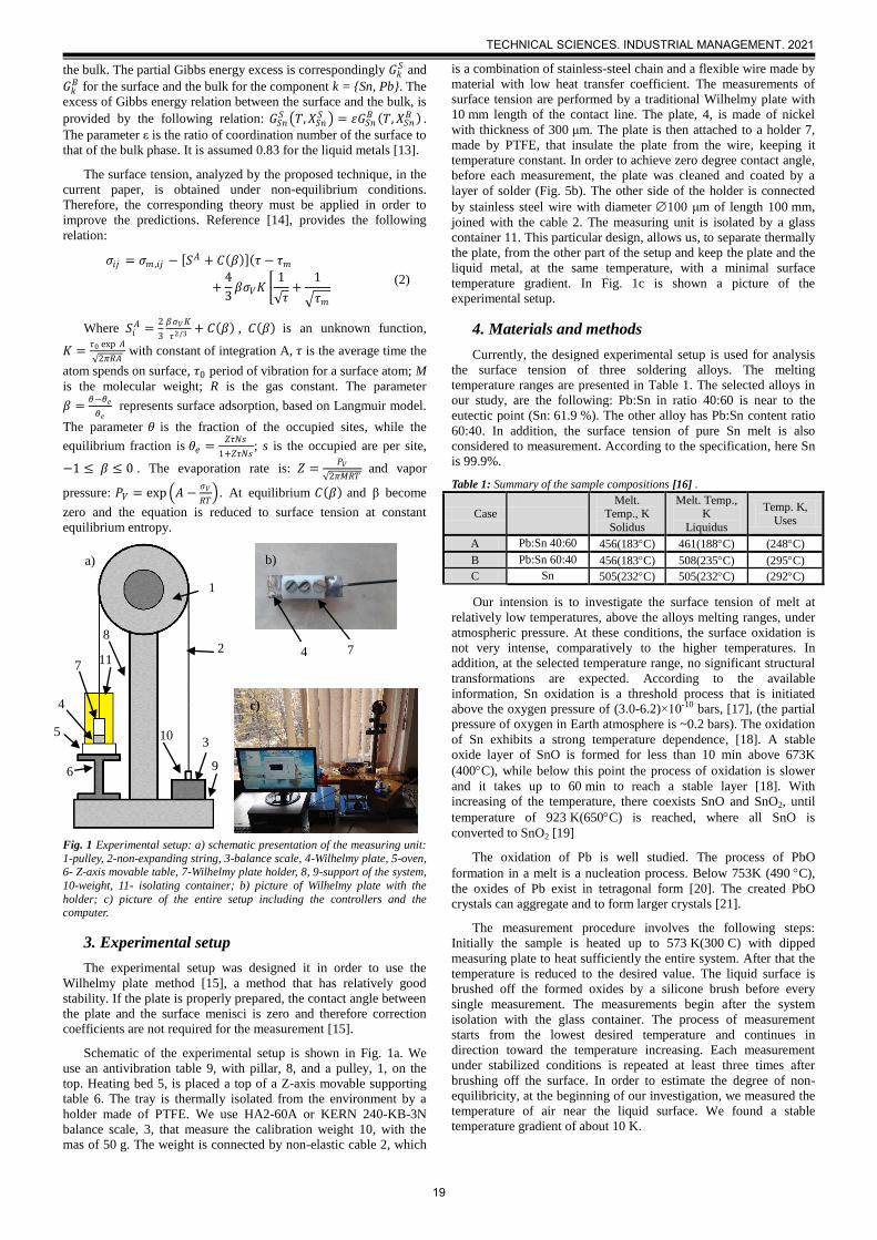
the bulk. The partial Gibbs energy excess is correspondingly 𝐺𝑘𝑆 and
𝐺𝑘𝐵 for the surface and the bulk for the component k = {Sn, Pb}. The
excess of Gibbs energy relation between the surface and the bulk, is
provided by the following relation: 𝐺𝑆𝑛𝑆 𝑇, 𝑋𝑆𝑛
𝑆 = 𝜀𝐺𝑆𝑛𝐵 𝑇, 𝑋𝑆𝑛
𝐵 .
The parameter ε is the ratio of coordination number of the surface to
that of the bulk phase. It is assumed 0.83 for the liquid metals [13].
The surface tension, analyzed by the proposed technique, in the
current paper, is obtained under non-equilibrium conditions.
Therefore, the corresponding theory must be applied in order to
improve the predictions. Reference [14], provides the following
relation:
𝜎𝑖𝑗 = 𝜎𝑚 ,𝑖𝑗 − 𝑆𝐴 + 𝐶 𝛽 𝜏 − 𝜏𝑚
+4
3𝛽𝜎𝑉𝐾
1
𝜏+
1
𝜏𝑚
(2)
Where 𝑆𝑖𝐴 =
2
3
𝛽𝜎𝑉𝐾
𝜏2/3+ 𝐶 𝛽 , 𝐶 𝛽 is an unknown function,
𝐾 =𝜏0 exp 𝐴
2𝜋𝑅𝐴 with constant of integration A, 𝜏 is the average time the
atom spends on surface, 𝜏0 period of vibration for a surface atom; M
is the molecular weight; R is the gas constant. The parameter
𝛽 =𝜃−𝜃𝑒
𝜃𝑒 represents surface adsorption, based on Langmuir model.
The parameter 𝜃 is the fraction of the occupied sites, while the
equilibrium fraction is 𝜃𝑒 =𝑍𝜏𝑁𝑠
1+𝑍𝜏𝑁𝑠; s is the occupied are per site,
−1 ≤ 𝛽 ≤ 0 . The evaporation rate is: 𝑍 =𝑃𝑉
2𝜋𝑀𝑅𝑇 and vapor
pressure: 𝑃𝑉 = exp 𝐴 −𝜎𝑉
𝑅𝑇 . At equilibrium 𝐶 𝛽 and β become
zero and the equation is reduced to surface tension at constant
equilibrium entropy.
Fig. 1 Experimental setup: a) schematic presentation of the measuring unit:
1-pulley, 2-non-expanding string, 3-balance scale, 4-Wilhelmy plate, 5-oven, 6- Z-axis movable table, 7-Wilhelmy plate holder, 8, 9-support of the system,
10-weight, 11- isolating container; b) picture of Wilhelmy plate with the
holder; c) picture of the entire setup including the controllers and the computer.
3. Experimental setup
The experimental setup was designed it in order to use the
Wilhelmy plate method [15], a method that has relatively good
stability. If the plate is properly prepared, the contact angle between
the plate and the surface menisci is zero and therefore correction
coefficients are not required for the measurement [15].
Schematic of the experimental setup is shown in Fig. 1a. We
use an antivibration table 9, with pillar, 8, and а pulley, 1, on the
top. Heating bed 5, is placed a top of a Z-axis movable supporting
table 6. The tray is thermally isolated from the environment by a
holder made of PTFE. We use HA2-60A or KERN 240-KB-3N
balance scale, 3, that measure the calibration weight 10, with the
mas of 50 g. The weight is connected by non-elastic cable 2, which
is a combination of stainless-steel chain and a flexible wire made by
material with low heat transfer coefficient. The measurements of
surface tension are performed by a traditional Wilhelmy plate with
10 mm length of the contact line. The plate, 4, is made of nickel
with thickness of 300 μm. The plate is then attached to a holder 7,
made by PTFE, that insulate the plate from the wire, keeping it
temperature constant. In order to achieve zero degree contact angle,
before each measurement, the plate was cleaned and coated by a
layer of solder (Fig. 5b). The other side of the holder is connected
by stainless steel wire with diameter 100 μm of length 100 mm,
joined with the cable 2. The measuring unit is isolated by a glass
container 11. This particular design, allows us, to separate thermally
the plate, from the other part of the setup and keep the plate and the
liquid metal, at the same temperature, with a minimal surface
temperature gradient. In Fig. 1c is shown a picture of the
experimental setup.
4. Materials and methods
Currently, the designed experimental setup is used for analysis
the surface tension of three soldering alloys. The melting
temperature ranges are presented in Table 1. The selected alloys in
our study, are the following: Pb:Sn in ratio 40:60 is near to the
eutectic point (Sn: 61.9 %). The other alloy has Pb:Sn content ratio
60:40. In addition, the surface tension of pure Sn melt is also
considered to measurement. According to the specification, here Sn
is 99.9%.
Table 1: Summary of the sample compositions [16] .
Case Melt.
Temp., K
Solidus
Melt. Temp., K
Liquidus
Temp. K,
Uses
A Pb:Sn 40:60 456(183C) 461(188C) (248C)
B Pb:Sn 60:40 456(183C) 508(235C) (295C)
C Sn 505(232C) 505(232C) (292C)
Our intension is to investigate the surface tension of melt at
relatively low temperatures, above the alloys melting ranges, under
atmospheric pressure. At these conditions, the surface oxidation is
not very intense, comparatively to the higher temperatures. In
addition, at the selected temperature range, no significant structural
transformations are expected. According to the available
information, Sn oxidation is a threshold process that is initiated
above the oxygen pressure of (3.0-6.2)×10-10 bars, [17], (the partial
pressure of oxygen in Earth atmosphere is ~0.2 bars). The oxidation
of Sn exhibits a strong temperature dependence, [18]. A stable
oxide layer of SnO is formed for less than 10 min above 673K
(400C), while below this point the process of oxidation is slower
and it takes up to 60 min to reach a stable layer [18]. With
increasing of the temperature, there coexists SnO and SnO2, until
temperature of 923 K(650C) is reached, where all SnO is
converted to SnO2 [19]
The oxidation of Pb is well studied. The process of PbO
formation in a melt is a nucleation process. Below 753K (490 C),
the oxides of Pb exist in tetragonal form [20]. The created PbO
crystals can aggregate and to form larger crystals [21].
The measurement procedure involves the following steps:
Initially the sample is heated up to 573 K(300 C) with dipped
measuring plate to heat sufficiently the entire system. After that the
temperature is reduced to the desired value. The liquid surface is
brushed off the formed oxides by a silicone brush before every
single measurement. The measurements begin after the system
isolation with the glass container. The process of measurement
starts from the lowest desired temperature and continues in
direction toward the temperature increasing. Each measurement
under stabilized conditions is repeated at least three times after
brushing off the surface. In order to estimate the degree of non-
equilibricity, at the beginning of our investigation, we measured the
temperature of air near the liquid surface. We found a stable
temperature gradient of about 10 K.
7
a)
c)
b)
7 4 11
2
1
4
5
6
3
8
9
10
TECHNICAL SCIENCES. INDUSTRIAL MANAGEMENT. 2021
19

The solidification of the analyzed specimens, after completion
of our set of measurements, is recorded by HDMI digital camera-
microscope with 3MP image sensor, resolution 102×1080, 1080P
with video recording speed 30fps. Its magnification range, by the
design, is 10x-220x.
5. Results and discussion
We performed measurement of the three alloys with declared
compositions in paragraph 4. The observed results, presented in Fig.
2, are quite interesting: Two cases provide very stable systematic
results: Pb:Sn in composition 40:60 and 60:40 (case A&B, Table 1).
The surface kinetics of Sn oxidation of the pure Sn liquid substance
did not allow proper measurements of surface tension with the
current configuration of our setup (case C, Table 1).
The results from our measurements showed that the surface
tension of Pb:Sn in ratio 40:60 is increased to values predicted by
Eq. (1) for pure Sn (compared to the data without oxidation, Fig. 1),
possibly because of formation of SnO. With increasing of the
temperature, the surface tension gradient is low. This result is
possibly because the oxidized Sn already dominates at the surface.
In the case with Pb:Sn ratio of 60:40, a formation PbO possibly
dominates at the surface, because at temperatures below 240C, Pb
partially separates. During the solidification, Pb is in excess (case B,
Table 1). On the surface it possibly reacts with atmospheric oxygen
and because of nucleation, formation of growing aggregates can
take place. In this case the surface tension is lowered to the
measured surface tension of pure Pb. A higher gradient with the
increasing of temperature is exhibit (comparing to the surface
tension at non-oxidizing conditions).
Fig. 2 Surface tension of Pb:Sn.
The performed experimental work allows to be analyzed the
non-equilibrium contribution to surface tension that comes from the
liquid surface oxidation. Based on the data, provided in Fig. 2 and
combination of Eq. (2ab) with Eq. (3), we can write [22]:
∆𝜎𝑖:𝑗 = 𝜎𝑖:𝑗 − 𝜎𝑚 ,𝑖:𝑗 (4)
Where 𝜎𝑖:𝑗 is the obtained theoretically surface tension from Eq.
(1) and 𝜎𝑚 ,𝑖:𝑗 is the measured value. Based on this we estimate
empirically the difference for Pb:Sn in ratio 40:60:
∆𝜎40:60 = 0.5249𝑇 − 380.68 (5a)
Correspondingly, for ratio Pb:Sn 60:40 is obtained:
∆𝜎60:40 = 0.0134𝑇 + 10.567 (5b)
In Eq. (5a) is shown that the adding surface energy rate because
of oxidation and non-equilibrium thermal conditions is much higher
in comparison to data in Eq. (5b). From the equations above is seen
that the mixture near the eutectic point (of Pb:Sn in 40:60) stabilizes
the surface tension as the added surface energy rate with increasing
of the temperature is very low. However, the measurements of pure
Sn (Table 1, C) surface tension indicated that the first several
minutes of Sn exposure on air, oxidation very actively takes place.
This is indicated visually by the changing of the color of surface to
yellow. Then, the formed oxide layer further stabilizes the surface
properties of the liquid melt and suppresses the further oxidizing of
Pb:Sn in ratio 40:60, contrary to the case 60:40, where is observed
stronger gradient of the surface tension decrease with the increasing
of the temperatures.
In order to understand better the processes, we recorded images
of the solidification process and presented them below. This is
helpful in providing a simple explanation of the obtained results.
The pictures in Figs 3-5 represent the solid alloys shortly after the
solidification of the investigated alloys, at the end of surface tension
measurement. The cooling was performed by turning off the heating
element and waiting the cooling of the samples to the ambient
temperatures, 293 K, (natural speed). We selected this approach to
cool the samples after several tests with controlled reduction of the
speed of cooling below the natural but no differences were observed
at the records of the surface solidification.
Figure 3 shows a picture of 60 % Sn and 40 % Pb sample
surface shortly after its solidification. The formed structure consists
from two constituent distinct phases: dark phase and crystalized
structure [23] [24]. The dark occupied relatively large zones consist
possibly from oxidized Pb, which remains on the surface. This
conclusion is based on the fact that after solidification of Sn (Fig. 5)
such dark phase formation is not observed.
Fig. 3 Solidified melt Pb:Sn in ratio40:60 (POK60).
Figure 4 represents the surface of cooled and solidified sample
of 40% Sn and 60% Pb near the melting point. It consists from two
solid phases. However, the mixture is formed in a very small scale,
and the phases are not distinguished on the picture. In our opinion,
oxidized Pb is dominating over the surface.
Fig. 4 Solidified melt Pb:Sn in ratio 60:40 ((POK40).
A picture of the solidified Sn is presented in Fig. 5. The
structure looks very much lamellar. The surface color of the
structure is nearly yellow at the solidification, which certainly
indicates that a thin layer of SnO is covering the surface upon the
oxidation.
y = -0.6019x + 871.24R² = 0.7864
y = -1.4281x + 1179.9R² = 0.926
300
350
400
450
500
550
600
650
460 480 500 520 540 560 580
Surf
ace
te
nsi
on
, mN
/m
Temperature, K
Sn
PbPb: 60%
Pb: 40%
MeasuredPb:Sn 60:40
MeasuredPb:Sn 40:60
Dark phase,
possibly PbO
TECHNICAL SCIENCES. INDUSTRIAL MANAGEMENT. 2021
20

For several minutes after exposure on air, just above the melting
point, the surface obtains this specific yellow color. At the
temperatures above 573 K, the color is changed to blue. This
surface color changing is attributed to the transformation of SnO to
SnO2 at higher temperatures.
Fig. 5 Solidified Sn melt.
6. Conclusions
Based on the performed studies of the surface tension, we
conclude that the proposed method of Wilhelmy plate is suitable for
measurement of liquid metal surfaces even under non-equilibrium
conditions. It is sensitive enough to be revealed the oxidation
surface properties. We detected strong surface kinetics in Pb
oxidation and the presence of oxidized Sn on the surface have the
opposite stabilization effect.
The presence of PbO on the surface is acting toward reduction
of surface tension in comparison with non-oxidized melt, while Sn
oxides modify the surface tension in opposite direction, in
comparison to the non-oxidized alloys. The significant Pb oxidation
decrease the surface tension to became nearly the same as the
surface tension of the pure Pb. The surface tension of the mixture
Pb:Sn 40:60 became nearly at the same range as the pure Sn (See
Fig. 2). The stabilization effects of oxidized Sn on the surface
tension should be investigated in future.
7. References
1. L. L. Bircumshaw, Phil. Mag, 17, 110, 181-191, (1934).
1. D. W. G. White, Metall. Trans. B, 2, 3067–3071, (1971).
2. M. Kucharski M, Arch. HUTN., 2, 22, 181-194, (1977).
3. K. Nogi, K. Oishi and K. Ogino, Mat. Trans., JIM, 20, 2, 137-
145, (1989).
4. W. Gasior, Z. Moser and J. Pstrus, J Phase Equilibria, 25, 1,
20-25, (2001).
5. I. Kaban, S. Mhiaoui, W. Hoyer and J.-G. Gasser, J. Phys.:
Condens. Matter, 17, 7867–7873, (2005).
6. E. A. Brandes and G. B. Brook, Smithells Metal Reference, 7-
th ed., Oxford: Butterworth–Heinmann, (1998).
7. Y. Xi, L.-J. Liu and Z.-H. Chen, Kovove Mater., 43, 432-439,
(2005).
8. Y. Kirshon, S. B. Shalom, M. Emuna, Y. Greenberg, J. Lee, G.
Makov and E. Yahel, MDPI materials, 12, 3999, (2019).
9. E. P. Loewen and A. T. Tokuhiro, J.of Nucl. Sci. and Technol,
40, 8, 614–627, (2003).
10. J. R. Weeks, Nucl. Eng. Des., 15, 363-72, (1971).
11. W. G. Gale and T. C. Totemeier, Eds., Soldering and Brasing,
in Smithells Metals Reference Book, 8-th ed., Academic Press,
34-1-34-22,.(2004),
12. J. A. V. Butler, Proc. Math. Phys. Eng. Sci., 348-375, (1932).
13. C. Maze and G. Burnet, Surf. Sci., 7, 411-418, (1977).
14. W. Contributors, Wilhelmy plate, Wikipedia, The Free
Encyclopedia, 19 December 2020. [Online]. Available:
https://en.wikipedia.org/w/index.php?title=Wilhelmy_plate&ol
did=989575010. (Accessed 2 February 2021).
15. An Avnet Company , https://www.farnell.com, 2019. [Online].
Available: http://www.farnell.com/datasheets/315929.pdf.
(Accessed 23 Jan. 2021).
16. A. Grigoriev, O. Shpurko, C. Steimer, P. S. Pershan, B. Ocko,
M. Deutsch, L. Binhua, M. Meron, T. Graber and J. Gebhardt,
Surf. Sci., 575, 3, 225-232, (2005).
17. E. Barreira, L. Pedrini, M. Boratto and L. Scalvi, Intl. J. of
Modern Phys. B, 34, 2050184-13p, (2020).
18. J. Geurfs, S. Rau, W. Richter and F. J. Schmiitte, Thin Solid
Films, 121, 3, 217-225, (1984).
19. T. E. Weyand , The oxidation kinetics of liquid lead and lead
alloys, University of Missouri--Rolla, (1970).
20. K. Gladinez, K. Rosseel, J. Lim,, A. Marino, G. Heynderickx
and A. Aerts, Phys. Chem. Chem. Phys., 19, 27593-27602,
(2017).
21. Y.-B. K. Kang, Calphad, 50, 23-31, (2015).
22. C. Basaran and R. Chandaroy, Appl. Math. Model., 22, 601-
627, (1998).
23. P. T. Vianco, S. N. Burchett, M. K. Neilsen, D. A. Rejent and
D. R. Frear, J. Elec. Materi., 28, 1290-1298, (1999).
TECHNICAL SCIENCES. INDUSTRIAL MANAGEMENT. 2021
21

Open innovation – potential, constraints and prospects
Borislava Galabova
University of Mining and Geology “St. Ivan Rilski”, Sofia, Bulgaria [email protected]
Abstract: In the last decades innovations are defined as main priority. Overtime they become an instrument for achieving economic growth
and social progress, increasing life standard and aiding in resolving difficult economic problems. The integration, globalization and
concurrence define the goal of business organizations to become more innovated, adaptive and flexible in order to never stop developing, gain concurrence advantages and preserve their market share. They always have to take into consideration the constant changing
conditions, the turbulent business environment and the increased consumer requirements for end products. In response of this necessity a new innovating model has been created and implanted, better known as open innovation. This relatively new modern concept show s
significant potential for developing and by doing this it finds a place in the business practice. By proving its effectiveness through achieving positive results, the open innovation is established as a successful and useful model for innovation, outlining different perspectives and new
routes for developing business organizations. Keywords:INNOVATION, OPEN INNOVATION, CLOSED INNOVATION, BUSINESS ORGANISATION, BUSINESS DEVELOPMENT,
ECONOMIC INNOVATION PERFORMANCE
1. Introduction
Over the past decade, innovation has been identified as one of
the main priorities. It is no coincidence that today they are accepted as a kind of vector of competitiveness and a logical path to the
creation of added value. Over the course of business history,
innovation has been established as a tool for achieving economic growth, increased living standards and social progress, helping to
solve complex economic and social problems. Increasing globalization, integration and competition justify the aspiration of
business organisations to be more innovative, open, adaptable and flexible in order to develop and protect their competitive advantages
and to stabilise their market positions. Moreover, they should continuously address the global challenges, the changing socio-
economic conditions, the turbulent environment and ever-increasing
consumer requirements. As a result, it becomes necessary to take into realization ideas that come not only from internal, but also from
external sources. It is the provision and accumulation of information from sources of different types and origins that plays a significant
role in increasing their innovation capacity, which predetermines future financial and economic performance. To this end, they must
constantly develop new or improved goods, services, business
models, technologies and know-how, be fully ready for innovation and be open to generate ideas. Some of them strive to be innovative
and "up-to-date" with the trends for creating, incorporating into and developing business ecosystems and platforms for open innovation
and shared resources and are oriented towards sharing the innovation process. Others focus on using their own ideas,
resources and research and development (R & D) potential. This closed and internally oriented innovation model delivers results
under certain conditions and remains up-to-date and applicable.
However, the turbulent economic development logically leads to the emergence of another open and rather externally oriented model,
which finds a place in business practice, and this makes it a subject of increased research interest.
2. Prerequisites and ways to solve the problem
The main problem is related to the discovery of the potentialand scope of open innovation, as well as to outlining the prospects
for the innovation process. The aim is to explore this potential for creating favourable conditions for the growth and development of
business organizations in the context of strong environmental
dynamics on national, European and international level. The subject of this research is open innovation - as a modern concept and model
for the conduct of the innovation process in business organisations.By comparative analysis and using a historical approach, a
comparison is made between open and closed innovations and brings out points of contact and fundamental differences. Based on
the use of analysis, summary, synthesis and analogy, some summaries of the scope, positive and possible negative aspects of
the open innovation model and its application from a business perspective are made. The emphasis is on the added value that the
model could provide. Various courses are sought for questions
about genesis, content and stages of the process and the potential of the open and closed innovation. Critical performance review and
analysis of good practices become the basis for identifying guidelines for the development of business organizations and
addressing serious issues, including ensuring competitiveness, added value, cost-effectiveness, growth and development.
3. Opportunities and potential of the open innovation
3.1. Open innovation: basics and conceptual framework
Historically, different theoretical views on innovation and
models for the innovation process have been discovered. On the basis of their comparison, several main types of innovation and
innovation process could be distinguished. The traditional innovation process is often described through a straight model in
which innovation is series of stages starting from R&D and ending with a product sold on the market [5]. But deeper analyses paint a
much more complex picture, it is difficult to argue that innovation is
going through a series of strictly defined, succesive stages [2]. Thus, compared to closed innovations, the non-traditional open
model of innovation process is not a linear process and is distinguished by different genesis, content and stages.
The concept of open innovation was first developed and
presented by Henry Chesbrouh in the early years of the 21st century. It rests on the perception that in a world flooded by
information, business organisations do not depend solely on their
own research and should not rely solely on it to achieve efficiency and competitiveness and to preserve and multiply their customers.
In order to be successful, they are forced to take advantage of a wider range of opportunities offered to them by external to the
organisation resources and ideas [4]. Open innovation has been proposed as an entirely new paradigm for managing innovation and
processes. According to this, the business organisations have
opportunities to combine internal and external ideas as well as internal and external paths to market to advance the development of
new technologies [4]. On this basis, the introduction and formalisation of the concept of open innovation aims in practice to
distinguish it from the closed innovation created in a traditional way. In the past, this type of innovation was meant by different
names, such as collective, partner, collaborative, modular and dispersed innovation. Since the beginning of the 21st century it has
become popular as an open innovation, which marks the beginning
of the construction of a comprehensive concept for this fundamentally different kind of innovation.
TECHNICAL SCIENCES. INDUSTRIAL MANAGEMENT. 2021
22

The concept of open innovation builds on the increased role of the external sources in the innovation process. Their growing role is
also accompanied by an expans ion of the organisation's R&D capacity, although this is not about internal capacity. There are
different ways of accessing and benefiting from external resources, making it possible to acquire, absorb and use knowledge, ideas and
concepts that are not a product of the activity of the business
organisation itself. In this way, it gets access to external creativity. The business organisation has the ability to use technology transfer,
shared resources, licensing, open source software and crowdsourcing, which are a field for the active flow of incoming
and outgoing information flow. By comparison, the traditional and widely used innovation model in the last century is most often
defined as closed because it concentrates and flows mainly within the organization. In order to be able to move smoothly from the
closed to the open innovation model and to take advantage of its
advantages and potential, business organisations must create, develop and establish an appropriate innovation climate by
monitoring, analysing and exploiting these opportunities fully under the right conditions. In this way, adaptation becomes key to
organisational competitiveness and business performance in the context of the set economic, social, political, legal, technological
and environmental variables.
The essence of the concept of open innovation is based on
overcoming and blurring organisational boundaries in order to generate ideas, develop and implement innovations. The
communication process is intensified between users, suppliers, researchers, partner and industry organizations, non-profit
organisations, even competitors whose behavior can be used as a barometer of the state, trends, attitudes and direction of business
development. Opening up and using an external perspective on the
process of generating ideas and turning them into innovations gives a new perspective and horizon to business organisations. The need
for constant change – as an iterative process, and its effective management become the basis for the imposition of open
innovation. On the other hand, the inability to have the organisational capacity to be large enough to ensure the progress of
innovation processes is a reason to increase the tendencies towards opening up business organisations and to look for new opportunities
for innovative development and management of change.
Prerequisites for the imposition of the new open model create globalisation, integration and increased mobility of workers, the
growth of the venture capital market and the increasing role and capacity of external suppliers. Business organisations face
significant changes related to and resulting from external environment factors, including the emergence and dissemination of
new technologies, accelerated technological transfer, major changes in economic, social, political, technical and cultural relations and
links, the transition from mass to individualised consumption,
increased competition along with cooperation and cooperation, shortening the life cycle of the product. The open innovation
approach is the new frontier to which we need to focus on the innovation process, but changes, both cultural, organisational and
institutional, which it implies should not be underestimated. The objective of its implementation is to reach stable market positions,
followed by business development and growth based on innovation
activity as a basic condition for increasing competitiveness.
Today low innovation activity and potential for innovation is a key feature, inherent both for the Bulgarian economy in its entirety
and for a significant part of the business organisations in particular. Their technological level lags behind that of competitors, which
outlines a vicious closed circle, leading to a further contraction of their innovation capacity and an impossibility of further growth and
development. These adverse circumstances are indicative and
relevant in the context of the need to "catch up" at the level of innovation and to align it with the other Member States of the
European Union. The long-term trend that has developed over the years does not allow for a significant improvement in the market
positions that Bulgaria has as a highly open economy, and has a negative impact on competitiveness. At the same time, the potential
for own research and development remains very limited compared to that of other economies. This raises a number of questions about
the real and potential opportunities for innovation that business organisations have and how much capacity they have and tend to
create and implement innovations in a more flexible way. Do their managers share the view that the openness of business organisations
is the key to achieving added value, efficiency and effectiveness?
Are they ready to transform, open their borders and work in broad collaboration with partners, building an open partner network?
Whether their answers are positive or negative, industrial structures continue to change and acquire a network form, which completely
changes the approaches to generating ideas, creating innovation and putting it into practice. Collaboration with external partners seems
to be particularly important with reference to social, organizational, and ethical issues in the context of innovation [3, 6]. In today’s
global society, firms recognise they have much to gain from
creating partnerships and engaging with the rest of the world [8, 9, 10]. A large number of practices fall within the scope of open
innovation and are instrumentalized through platforms [7]. Their use is becoming increasingly popular and preferred because it
allows the sharing of the innovation process, resources, ideas and solutions and the involvement of more participants.
3.2. Comparative analysis of the concepts of the closed and open innovation
Understanding the nature of open innovation requires
comparing it with the traditional closed version. The search for the common and the different between the two concepts is the basis for
analysis and evaluation of these different models.
The concept of closed innovation is based on the research and
development of the business organisation itself. In this case, the ideas and solutions to problems are generated and developed
without crossing its boundaries, which are poorly permeable. (Fig.1).
Research Development
Boundaries of the company
Research Market
projects
Fig.1 Paradigm of the closed innovation Cresbrough, H. (2003). Open innovation: The new imperative for
creating and profiting from technology. Boston, Harvard Business Press
As shown in Fig. 1, this type of innovation is a result of the
efforts mainly of a particular business organisation and are a logical
consequence of its investment and innovation activities. Innovation is therefore a function of its own research, financial and human
potential. In order for the business organisation to make the most of R&D, all phases of the innovation process are deployed and carried
out within its framework and on the basis of the use of internal resources, including human resources. If there is a need for further
expertise, external experts are rarely attracted. In general, the main
part of the R&D activity is carried out within the organisation by the internal experts involved in the generation and development of
innovative ideas. Thus, the model for innovating from the beginning of the idea to its practical implementation is rather centralized and
focused on the organization itself and its structures. In today's innovation context, significant organisational potential is needed in
all its aspects, making it difficult for innovation processes to take place and slowing down the receipt of expected results, whether
products, services, processes or business models. The researchers
on the subject agree with the view that this is also the largest deficit
TECHNICAL SCIENCES. INDUSTRIAL MANAGEMENT. 2021
23

of the closed innovation model. Focusing mainly on the internal capacity and viability of the business organisation to create both
novelty, utility and added value is equal to limited innovation opportunities that extend to the organisational capacity itself.
Despite this major disadvantage, the closed innovation model also has advantages. It continues to work well and show results in
certain circumstances and in certain areas of business. For a
concrete business organization advantages originate from the relative independence from the external environment, partners and
collaborators and their freedom to generate and formulate their own ideas and solutions to the problems without being strongly or
entirely dependent on external sources of ideas and resources needed to the innovation activities.
The shortcomings arise from the fact that the knowledge
generated is relatively incomplete and fragmented, as it is created
within the organisation’s boundaries and according to its capacity and resources, which are in any case limited. Regardless of its size
and internal potential, no organization by itself has sufficient financial, human, material, temporal and information resources to
solve the emerging complex theoretical and applied problems. Sharing resources and creating innovation based on cooperation are
an objective necessity if the business organisation strives to achieve results and be relevant to realities. Finding realistic, feasible and
effective solutions to such problems implies large-scale, long-term
and costly development and research that requires significant capacity, pooling of resources and strategic management. For these
reasons, closed innovation faces more and more barriers in its application and development. Problems seeking solutions are
complicated, and solving them without multilateral cooperation becomes difficult, even impossible, and greatly becomes more
expensive.
Research Development
New market
Boundaries of the company
Research Present market
projects
Fig. 2 Paradigm of the open innovation
Cresbrough, H. (2003). Open innovation: The new imperative for creating and profiting from technology. Boston, Harvard Business
Press
The concept of open innovation is based on opening up the business organisation to the external environment. As shown in Fig.
2, ideas, views and suggestions of various direct or indirect actors in the innovation process begin to pass through its boundaries. Open
innovation has been established in practice since the beginning of
the 21st century and is particularly relevant in today's conditions. Trends of increasing opening up to consumers and their direct or
indirect involvement in innovation generation process lead to their entry and enforcement into practice.
Open innovation is a result of diverse forms of exchange of
ideas, ready-made solutions for creating innovations and cooperation in their creation together with various external
organizations, including partner business organisations, universities,
research institutes, units and centers, public sector representatives, freelance experts, spin-off companies and consummers. In case of
open innovation both internal and external experts and collaborators are included. The organisation uses them to achieve certain results
leading to innovations or improvements of an existing product, service, business process or model. The range of participants in the
process should be wide in order to cover many ideas, solutions and proposals to overcome a specific challenge formulated as a
problem. The open innovation concept also includes the active
presentation of knowledge by the company in the form of the sale of rights to use its intellectual property [1]. The aim of this model is to
achieve innovation in the most active, flexible and decentralised way, innovation is gradually needed in practice, together with its
different practical modalities.
Over the past decade, the list of organisations from different
fields of activity using this approach in practice has become longer. This is no coincidence, as the assessment of organisational
resources and opportunities leads to a re-appreciation of the constraints of the closed innovation and the potential benefits of
opening, searching for and sharing resources and using them. The model aquires new reading and become even more actual in the
current contex related to the coronavirus pandemic (COVID-19), the crisis and recession, which are direct consequence of it.
Cooperation between business organisations from different fields of
activity becomes imperative and objectively justified in order to find solutions to the emerging problems and issues in all aspects of
the economy and society. Given the adaptive, accessible and flexible model, open innovation shows potential to expand the value
creation space. They can help build a positive image, defined by greater transparency and openness of the organization's activities.
3.3. Open innovation process
Chronologically the open innovation process goes through several main stages. First, it is predestined by the generation of a
realistic and feasible idea related to a need, which is an initial stage
for each innovation. A significant condition for starting is the existence of an unresolved problem for which there are objective
and actual prerequisites and possibilities to be resolved in perspective and so the need can be met. The innovation idea should
also be related to the achievement of a specific objective of the business organisation. It is defined by its potential and available
resources through which to develop and become a finished product on the market. Secondly, it follows a stage of development and
implementation of the idea, assessed as realistic, feasible and
consistent with the objectives and restrictive conditions arising from the characteristic of the internal and external environment. Third,
the process ends with the marketing idea, which has become a specific innovation product bearing the hallmarks of novelty, utility,
value and value.
The creation of open innovation is a systematically ongoing process that has different stages and participants in each of them. In
the first stage named conceptualization it is necessary to create
prerequisites for establishing an organizational climate suitable for creating an open innovation. Often the stage of generation of the
idea itself is most open and there is an opportunity to participate directly or indirectly a large number of participants. Within its
framework, important activities are carried out: research planning, targeting, ensuring innovation infrastructure, organization of the
team, allocation of roles, resources to carry out their activities and tasks and manage them. The first stage ends only when a
comprehensive concept has been built and a work plan has been
developed towards it. The conceptualisation phase should not be underestimated because it is the basis for moving to the next stages
and therefore affects their results and starting points. Unlike closed innovation, during the conceptualisation phase of open innovation,
it is necessary to plan and anticipate the normal flow of incoming and outgoing information flows from the point of view of business
organisations, as well as to clarify the overall vision, purpose and
way of achieving it. For this purpose, the necessary models and tools are developed, the competences are specified and the project is
prepared. For the development stage, as a starting point, the results achieved from the conceptualisation stage shall be used. The third
stage is the implementation. Within its framework, the system begins to "work" and the processes are carried out according to the
planned in the conceptualization stage and the prepared project in the development stage. In this final stage, the most active exchange
of information takes place between the business organization,
stakeholders and its partners in the innovation process. By
TECHNICAL SCIENCES. INDUSTRIAL MANAGEMENT. 2021
24

implementation of some guiding mechanisms, innovation activities allow to go beyond organisational boundaries and achieve process
efficiency. A significant difference between the closed and open model of innovation is found precisely in controlling the process at
different levels and the degree of control. Closed innovation has significant control, concession and centralisation of resources, little
interaction with the outside world and environment and
impermeable boundaries. Compared with them, open innovation has significantly weaker control, weak concentration and strong
decentralisation of resources, active interaction with the outside world and environment and permeable organisational boundaries. In
general, the process of innovation undergoes a principled transformation - from individual becomes collective and from a
straight becomes non-straight. It seeks a balance between cooperation on the one hand and competition on the other.
3.4. Challenges and constraints on open innovation and approaches to addressing them
Finding new partners and creating partner networks doesn't just bring positives. It also means more costs for the business
organization concerned. However, the creation of a partner network
and its expansion provides new opportunities for development and growth and revenue. In parallel, the new partners also provide
additional skills and competencies in the direction of shared resources and expand the prospects for the business organization. In
the current context, requiring all businesses to adapt to new realities and overcome the effects of the coronavirus pandemic (COVID-19),
finding partners is facilitated by focusing on a common problem. This way, organisations can navigate the search for more new
partners and types of partners. In this sense, the main challenges
and constraints to open innovation stem from the need to transform business organisations and their orientation towards an open and
multilateral innovation process, which also means a fundamentally new strategy for managing it. The lack of practice and experience in
building and developing a partner network can also be attributed to possible challenges, because starting from scratch will involve
additional costs and time to build it and the actual start of the innovation process. The issue of intellectual property and its
protection is also challenging in regard of the changes in strategy
and organisation needed in the transition to an open innovation model. Although these challenges and constraints are real. They can
be overcome or reduced if appropriate management strategies, methods and techniques are implemented in a timely and effective
manner.
4. Results and discussion
Opening up business organisations to the outside world and
transforming models from closed to open ones is a fact. Proving its effectiveness in recent years, open innovation is necessary as a
successful, useful and applicable innovation model, which is widely
embraced first in developed and then in developing countries. A prerequisite for its entry are the wide range, flexibility and
adaptability that the open model offers and which are necessary for the development of innovation activity in the face of significant
dynamics and increased competition. Invariably, the current conditions require radical changes in the strategies, orientation,
approaches and models of business organisations to the innovation process and their relations with consumers, partners and
competitors. The search for ideas for solutions to consumer
problems is no longer only a novelty, but is considered to be an objective necessity. Turning them into innovators is a key to the
success of those business organisations that strive to be innovative, seek new paths for growth and development and increase their
innovation capacity. The adoption of open innovation strategy, created on a broad and open basis, and its implementation give
business organisations certain advantages: an opportunity to achieve
greater added value and benefit for society and the individual consumer, greater consumer satisfaction and a more effective
innovation process. The interaction and exchange of ideas between many different participants gives a new look to the innovation
process and expands not only its boundaries, but also the desired end effects of the development and implementation of innovations.
The aim is to open new business opportunities and to increase the efficiency of the innovation process by reaching empty spaces and
proceeding to their research and utilization. The main direction for
development is the imposition of a strategy for opening the innovation process, if not fully, at least partially for certain areas of
activity, goods, services, processes and models in order to make the most of the opportunities of the external environment and the
potential of the concept of open innovation.
5. Conclusion
This analytical study is dedicated to the potential of the open
innovation to create favorable conditions for growth and development of business organisations in the context of strong
environmental dynamics at national, European and international level and to facilitate adaptation to economic, social, technological,
technical and political conditions. Different perspectives are sought
on the genesis, content and stages of the process and the potential and scope of open innovation compared to closed innovation. The
aim is to study the potential for creating favorable conditions for growth and development of business organisations, as well as to
identify the main challenges in the implementation of such open models. It is concluded that open innovation offers new business
horizons, increasing the efficiency of the innovation process,
reaching empty spaces and proceeding to their study and utilization. A key direction for business development is the imposition of a
strategy to open up the innovation process, if not entirely, at least in part, to certain areas of activity, goods, services, processes and
models in order to harness the opportunities coming from the external environment and to exploit the potential of the concept of
open innovation.
References
1. Бичурова, И. Класификация на иновациите. KNOWLEDGE –International Journal Vol. 30.1, March, 2019 / Bichurova, I.
Classification of innovations. KNOWLEDGE – InternationalJournal Vol. 30.1, March, 2019
2. Манолов, В.Исторически преглед на моделите за протичане
на иновационните процеси, e-Journal VFU, Issue 10-2017,https://ejournal.vfu.bg/bg/pdfs/VManolov_Statia_4_22.12.2016.pdf
/ Manolov, B. Istoricheski pregled na modelite za protichane nainovacionnite procesi, e-Journal VFU, Issue 10-2017,
https://ejournal.vfu.bg/bg/pdfs/VManolov_Statia_4_22.12.2016.pdf3. Arnold, M. The role of open innovation in strengthening
corporateresponsibility. International Journal of Sustainable
Economy, 3(3), 2011, p. 361–3794. Cresbrough, H. Open innovation: The new imperative for
creating and profiting from technology. Boston, Harvard BusinessPress, 2003
5. Coombs, R. et al. Economics and Technological Change.Rowman & Littlefield, 1987
6. Hossain, M. Open innovation: So far and a way forward. WorldJournal of Science Technology and Sustainable Development,
10(1), 2010, p. 30–41
7. Isckia, T. Ecosystemes d’affaires, stratégies de platform etinnovation ouverte: vers une approche integrée de la dynamique
d’innovation . Management & Avenir, 2011/6, № 46, p. 157-1768. Håkansson, H., & Snehota, I. No business is an island – The
network conceptof business strategy. Scandinavian Journal ofManagement, 5(3), 1989, p. 187–200
9. Huizingh, E. K. R. E. Open innovation: State of the art and future
perspective.Technovation, 31(1), 2011, p. 2–9 10. Stanko, M. A. et al. Under the wide umbrella of openinnovation.
Journal of Product Innovation Management, 34(4), 2017, p. 543–558
TECHNICAL SCIENCES. INDUSTRIAL MANAGEMENT. 2021
25

Приложение на различни цветови системи за определяне визуални характеристики
на бира
Application of different color systems to determine the visual characteristics of beer
Христина Андреева1,*, Владимира Ганчовска1, Радослава Габрова1
Университет по хранителни технологии Пловдив, бул. Марица 26, България1
Abstract: The main characteristics for assessing the appearance of beer and various possibilities for their determination are considered. The
possibility of detecting quality indicators using digital image processing is presented. The NI Vision Assistant software environment is used
and the features of its available color systems RGB, HSI, HSV and HSL are studied. The influence of the extraction of the different color
components on the precise separation of the considered indicators of beer is presented. From the obtained results it was found that some of
the grayscale images are similar and applicable for segmentation and determination of the required characteristics.
Keywords: COMPUTER VISION, BEER, NI VISION ASSISTANT, COLOR SYSTEM
1. Въведение
Бирата е едно от най-широко консумираните напитки по
света [1]. Основните съставки при производството на бира са:
вода; малцов ечемик, но може да се използват и пшеница, ръж,
царевица, ориз, овес, сорго, лимец; бирена мая, необходима за
ферментацията; хмел, който ароматизира, придава горчивина и
действа като природен консервант. При някои видове се
използват допълнителни съставки, като билки и плодове, за
добавяне на други аромати и вкус.
Всяка бира се отличава със специфични за марката външен
вид, аромат, вкус и текстура. Едно от първите неща, които
потребителите оценяват е външния вид, който се свързва с
показатели като цвят, бистрота и пяна на продукта. Пяната се
образува от появата, издигането и освобождаването на газови
мехурчета и се оценява се чрез нейната височина, стабилност
(дълготрайност) и структура (размер и разпеделение на
балончетата). Стабилността на пяната е важно качество на
бирата, тъй като пяната се явява ефективна повърхност за
обмен на газ и насочва ароматите към обонятелните сензори на
пиещите [2].
Редица учени са насочили своите разработки към
възможности за определяне на показатели качеството на бира
[3, 4, 5, 6, 7, 8].
В своя разработка James J. Hackbarth [3] предлага
проследяване на затихването на бирената пяна на шест марки
бира. За целта е използван прозрачен стъклен цилиндричен съд
с вместимост 400 ml. В продължение на 5 минути от
наливането на бирата са направени измервания на пяната. По
време на първата минута са правени замервания на всеки 15
секунди, а след това на всеки 30 секунди. Така получените
резултати са обработени и е установено, че първоначалното
спадане на пяната (30-45 сек.) не е с експоненциална
зависимост, докато данните след това време следват
експоненциално затихване.
Arnd Leike [4] предлага изчисляване на константата на
разпадане на бирена пяна за разграничаване на различни бири.
Проверена е последователността на теоретичните модели с
получените данни, направена е оценка на параметрите и
определяне на доверителните интервали.
Jasmina Lukinac и екип [8] предлагат замяната на
инструментално измерените показатели на бирата с
автоматична, обективна и бърза оценка, чрез приложение на
компютърно зрение.
В настоящата статия е разгледана възможността за цифрова
обработка на изображения, с цел извличане на показатели на
бирата. Изследвани са различни цветови пространства и
извличането на тяхна компонента върху ясното отделяне на
изследваните показатели – ниво на течността и ниво на
бирената пяна.
2. Материали и методи
С помощта на цифрова камера е заснет видеоклип с
продължителност 5 мин. от сипването на бира в цилиндрична
чаша с вместимост 330 ml. Направено е нарязване на кадри на
всеки 5 сек. Така получените изображения се използват за
автоматично определяне характеристики на бира като
количество на течната фаза и на пяната. За целта е необходимo
да се избере подходяща цветова система за работа и да се
направи извличане по някоя от нейните компоненти. За
обработката на изображения е избрано да се работи с NI Vision
Assistant. Наличните цветови системи за работа са RGB, HSI,
HSV и HSL.
RGB цветова система
Maxwell, Young и Helmholtz защитават трихроматичната
теория. Тя се основава на твърдението, че има три вида
фоторецептори, приблизително чувствителни към червената,
зелената и синята област на спектъра [9]. RGB цветовото
пространство използва комбинация от червена, зелена и синя
светлина с различна степен на яркост за получаване на всеки
цвят [10, 11, 12]. Смята се, че този цветови модел е най-близък
до човешкото възприятие, тъй като в човешкото око има
рецептори, които реагират точно на тези цветове. Ако трите
цвята се припокрият се получава бяло. По тази причина RGB
цветовия модел включва и точка на белия баланс и крива за
корекция на гамата [10]. Всяка една от трите компоненти заема
може да бъде със стйности в диапазона от 0 до 255. За удобство
е прието, че всички цветови стойности са нормализирани и
могат да се представят с единичен куб (фиг. 1) [13].
Фиг. 1 Графично представяне на RGB цветови модел
HSI цветова система
Цветовият модел HSI се описва чрез компонентите –
цветови тон, наситеност и интензивност (фигура 2) [14]:
• Hue – цветовият тон е чистия цвят на светлината. Това е
преобладаващия (доминантен) цвят, който виждаме. Измерва
се с разположението на цвета в цветовия кръг, от който се
вижда, че червеното се намира на 0 градуса, жълтото на 60,
TECHNICAL SCIENCES. INDUSTRIAL MANAGEMENT. 2021
26

зеленото на 120, циан на 180, синьото на 240 и магента на 300
градуса;
• Saturation – наситеността е силата и чистотата на цвета. Тя
представя количеството сиво в цвета и се променя от 0 (сиво)
до 1 (наситен цвят);
• Intensity – интензивността е параметър, определящ
осветеността или затъмнеността на цвета. Всички цветове от
цветния кръг имат максимална интензивност (100%)
независимо от тона. Намаляването на интензивността на цвета
означава неговото затъмняване. Тази координата е вертикална
(в интервала 0 до 100%). В резултат се получава цилиндър или
конус, ако се премахнат черните цветове. Образуват се серия
кръгове (сечения) с намаляваща яркост, от които най-долния
слой е черен.
Фиг. 2 Графично представяне на HSI цветови модел
HSV цветова система
Друг често използван цветови модел е HSB модела, който е
представен графично на фигура 3. Той е разновидност на
цветовия модел HSI и се описва чрез трите основни
характеристики на цвета:
• Hue (нюанс) – измерва се с положението на цвета в
цветовия кръг, задава се в градуси от 0 до 360. Най-често
нюанса се задава с името на цвета – червен, оранжев, зелен;
• Saturation (наситеност) – силата и чистотата на цвета.
Наситеността представя количеството сиво в цвета, измерва се
в процент от 0 (сиво) до 100 (наситен цвят). В стандартния
цветови кръг, наситеността нараства от центъра към краищата;
• Brightness (осветеност) – измерва се в проценти от 0
(черно) до 100 (бяло).
Този модел е познат и като HSV (Hue, Saturation, Value)
цветови модел, където цветовата компонента Value има същите
стойности и смисъл като компонентата Brightness [15].
Фиг. 3 Графично представяне на HSB цветови модел
HSL цветова система
Друга разновидност на HSI модела е HSL, който е
съкращение от Hue /цветови тон/, Saturation /наситеност/ и
Luminance /осветеност/. Осветеността определя количественото
участие на черната съставка в разглеждания цвят 0 до 100 [16].
На фигура 4 са представени графично HSL и HSV цветови
модели.
Фиг. 4 Графично представяне на HSL и HSV цветови модел
За преобразуване на изображението от цветно в полутоново
се използва извличане по една от компонентите в различни
цветови системи. На фигура 5 е представен пример за
преобразуване от цветно в полутоново изображение при RGB
цветова система [17]. В първата колона са представени
съответните изолирани цветови компоненти в естествени
цветове, а във втората са техните еквиваленти в сивата скала.
Полутоновото изображение се използва за разграничаване на
обектите на преден план от фона (сегментация).
Фиг.5 Преобразуване от цветно в полутоново изображение
3. Резултати и обсъждане
След получаването на цветни изображения е необходимо
тяхното преобразуване в полутоново. Изследвани са
различните цветови системи (RGB, HSL, HSV, HSI) и
влиянието от извличането на всеки един от компонентите
върху ясното оделяне на течната фаза и бирената пяна. От
получените резултати е установено, че част от полутоновите
изображения са незадоволителни и неприложими за измерване
на желаните показатели. На фигура 6 са представени резултати
от преобразуването на изображение от цветно в полутоново
при извличане на цветовите компоненти Hue и Saturation.
Фиг. 6 Полутонови изображения при извличане на компонентите H –HSL и S-HSL
TECHNICAL SCIENCES. INDUSTRIAL MANAGEMENT. 2021
27

При RGB цветовата система с извличането на
компонентите се получават полутонови изображения с много
близки резултати. При останалите цветови системи HSL, HSV
и HSI също се наблюдават сходни резултати, съответно за
компонентите: Luminance, Value и Intensity. Резултати от
извличането на Green компонента от RGB цветовото
пространство и Luminance от HSL са представени на фигура 7.
Фиг. 7 Полутонови изображения при извличане на компонентите
G –RGB и L-HSL
4. Заключение
С извличане на една от цветовите компоненти Red, Green
или Blue при RGB цветова система се получава полутоново
изображение със сходен резултат. Резултатите от
преобразуването на цветните изображения, чрез извличане на
компонентите Luminance, Value и Intensity съответно за HSL,
HSV и HSI цветова система, са сходни. Полутоновите
изображения, получени чрез изброените компоненти за
съответните цветови системи, са приложими за сегментиране и
отчитане на характеристиките течна фаза и бирена пяна.
5. Литература
[1] Arnold, J. P., Origin and History of Beer and Brewing: From
Prehistoric Times to the Beginning of Brewing Science and
Technology, BeerBooks.com, (2005)
[2] Bamforth C., I. Russell, G. Stewart. Beer: A Quality
Perspective (Handbook of Alcoholic Beverages) 1st Edition,
Series: Handbook of Alcoholic Beverages. Academic Press,
(2008)
[3] Hackbarth, J. J.,Multivariate analyses of beer foam stand,
Journal of the Institute of Brewing 112.1: 17-24, (2006)
[4] Leike, A., Demonstration of the exponential decay law using
beer froth, European Journal of Physics 23.1: 21, (2001)
[5] Viejo, C. G, et al., Development of a robotic pourer
constructed with ubiquitous materials, open hardware and
sensors to assess beer foam quality using computer vision and
pattern recognition algorithms: RoboBEER, Food Research
International 89: 504-513, (2016)
[6] Gonzalez Viejo, C., et al., Development of Artificial Neural
Network Models to Assess Beer Acceptability Based on
Sensory Properties Using a Robotic Pourer: A Comparative
Model Approach to Achieve an Artificial Intelligence System,
Beverages 5.2, (2019)
[7] Baxter, E. D., P. S. Hughes, Beer: Quality, safety and
nutritional aspects, Royal Society of Chemistry, (2001)
[8] Lukinac, J., et al., Computer Vision Method in Beer Quality
Evaluation — A Review, Beverages 5.2: 38, (2019)
[9] Heesen, R., The Young-(Helmholtz)-Maxwell Theory of Color
Vision, URL: http://philsci-archive.pitt.edu/id/eprint/11279
(accessed 28.02.2021 ) (2015)
[10] Pascale, D., A review of rgb color spaces... from xyy to
r’g’b’, Babel Color 18: 136-152, (2003)
[11] Gonzalez R., Digital Image Processing, Prentice-Hall, New
Jersey, ISBN:0-201-18075-8, (2002)
[12] Pratt W., Digital image processing: PIKS Inside, Third
Edition, Copyright John Wiley & Sons, Inc., ISBNs:0-471-
37407-5 (Hardback); 0-471-22132-5 (Electronic) (2001)
[13] Ren J., Yuli Shen and lei Guo, A Novel Image Retrieval based
on Representative Colors, Palmerston North, November (2003)
[14] Chien Ch., Din Chang Tseng, Color image enhancement with
exact HSI color model, International Journal of Innovative
Computing Information and Control, ICIC International©,
ISSN 1349-4198, pp. 6691-6710, (2011)
[15] Dongqing L., HSV Color Space, Encyclopedia of
Microfluidics and Nanofluidics. Springer, Boston, MA.
https://doi.org/10.1007/978-0-387-48998-8_656, (2008)
[16] Hue vs Color, http://thelandofcolor.com/hue-vs-color/,
(достъпно на 28.02.2021 г.)
[17] Shahriar Y., Introduction in Image Processing Matlab
Toolbox,
https://www.slideshare.net/ShahriarYazdipour/introduction-in-
image-processing-matlab-toolbox (достъпно на 28.02.2021 г.)
TECHNICAL SCIENCES. INDUSTRIAL MANAGEMENT. 2021
28

Приложение на компютърно зрение за определяне на големина и разпределение на
добавки в кексчета
Application of computer vision to determine the size and distribution of additives in cakes
Христина Андреева1,*, Владимира Ганчовска1
Университет по хранителни технологии Пловдив, бул. Марица 26, България1
Abstract: This article discusses a computer method for determining the size and distribution of additives (pieces of chocolate) in cupcakes.
Images of the previously cut cupcakes are taken with a digital camera. An algorithm and program are developed for the processing of the
obtained images in the NI Vision Builder and NI Vision Assistant environments. The percentage of additives on the cut surface of cupcakes is
determined. The coefficient of non-uniformity is calculated and a threshold is chosen against which the samples can be divided into two
categories – with uniform and with uneven distribution of additives. The proposed computer image processing can be applied to other dough
products for quantitative and objective assessment of the uniformity of distribution of additives in them.
Keywords: COMPUTER VISION, ADDITIVES, CAKES, NI VISION BUILDER, NI VISION ASSISTANT
1. Въведение
Кексчетата са сладки печени тестени продукти, които се
състоят от сложна смес от взаимодействащи съставки, основно
захар и променливо количество на мазнини, брашно, яйца и
бакпулвер, които имат типична пореста структура и голям
обем. Потребителите изискват структурата им да е мека,
гъбеста и нежна [1].
За определяне качеството на продукта се използват
инструментални методи, които описват текстурата на печените
изделия [2]. Тези методи са разрушаващи и субективни. За по-
обективно определяне на качеството се използват съвременни
компютърни методи за анализ на изображения [3, 4, 5].
Тяхното приложение е за оценяване на външни характеристики
на кексчета като цвят и обем [6, 7]. Използват се също и за
оценяване на разрезната повърхност като дебелина на кората и
степен на шупливост [8, 9].
Редица учени използват компютърното зрение като метод
за оценка на външният вид на кексчета [6, 7, 8, 9].
Анализът на изображения е използван за определяне срок
на годност на тестени изделия [6]. Oscar Grillo и екип предлагат
измерване на разликите в сивите, червените, зелените и сините
стойности между началото и края на времето за съхранение.
Използвани са изображения и хистограмите на съответните
цветови компоненти.
В [9] е предложен анализ на изображения на надлъжен и
напречен разрез на кексчета за оценка влиянието на
количеството полидекстроза и сукралоза (PD-SC), заместващи
захарозата (50% PD-SC и 100% PD-SC) върху тяхната
шупливост.
В настоящата статия са представени алгоритъм и програма,
които откриват количеството шоколадови парченца върху
разрезната повърхност на кексчета. Предложен е метод за
оценка равномерността на разпределение на добавките.
2. Материали и методи
За експерименталната работа са използвани кексчета с
добавени парченца шоколад, закупени от търговската мрежа. С
помощта на цифров фотоапарат OLYMPUS PEN Mini E-PM1 са
заснети разрязаните наполовина кексчета. С помощта на статив
е осигурено еднакво работно разстояние между камерата и
разрезната повърхност на пробите. Изображенията с
резолюция 4032x3024 са съхранени в .JPG формат. За
измерване на количеството добавки (парченца шоколад) в
кексчетата и тяхното разпределение по разрезната повърхност
е създадена програма в програмни среди NI Vision Builder и NI
Vision Assistant. Програмата следва алгоритъм представен на
фигура 1.
Фиг. 1 Блок-схема на алгоритъма за обработка на изображения
След зареждане на първичното изображение е направено
пространствено калибриране с цел преминаване към реални
мерни единици (mm).
Създадена е подпрограма за бинаризиране и отделяне на
разрезната повърхност на кексчето от фона. Използвана е
морфологичната операция „запълване на дупки“ за
пренебрегване на шуплите и добавките в кексчето. За
пренебрегване на смущения като отблясъци и малки трохи в
областта на фона е приложена морфологичната операция
„премахване на малки обекти“. Резултат от подпрограмата,
представен на фигура 2, е бяло изображение на разрезната
повърхност върху черен фон.
Фиг. 2 Резултат от преобразуването на изображението от цветно в
черно-бяло
С помощта на функционални инструменти за измерване във
Vision Builder са определени най-левият, най-десният, най-
горният и най-долният пиксел от разрезната повърхност на
кексчето. Спрямо тези граници е дефинирана областта на
интерес и в центъра ѝ е позиционирана правоъгълна
Зареждане на изображение
Пространствено калибриране
Подпрограма за отделяне на разрезната
повърхност от фона
Дефиниране на разрезната
повърхност като област на интерес
Позициониране на координатна система
Определяне на броя пиксели от разрезната повърхност
Дефиниране на 4 равни области на
интерес
Определяне на брой пиксели от разрезната
повърхност за всяка област
Подпрограма за отделяне на добавки
на преден план
Определяне броя пиксели на
добавките за всяка област
Съхраняване на резултати
TECHNICAL SCIENCES. INDUSTRIAL MANAGEMENT. 2021
29

координатна система. Определен е броят на белите пиксели от
изображението. Спрямо координатната система са дефинирани
четири еднакви области на интерес. Тяхната последователност
е представена на фигура 3. За всяка от четирите области на
интерес е определен броят на пикселите с бял цвят.
Фиг. 3 Дефиниране на четири зони на интерес
За отделянето на добавките на преден план е създадена
подпрограма, която зарежда отново входното цветно
изображение. Избран е праг за бинаризиране, който оцветява в
бял цвят добавките и част шуплите в кексчето. С цел
отстраняване на част от шуплите е използвана
морфологичната операция „премахване на малки обекти“.
Резултат от подпрограмата е представен на фигура 4.
Фиг. 4 Резултат от отделянето на добавки на преден план
Определени са броят на пикселите с бял цвят само за
добавките в кексчето, както за цялата разрезна повърхност,
така и за дефинираните четири области. За целта е използван
критерият обектите да са с размер по-голям от 10 mm2.
Критерият е съобразен с реалните размери на парченцата
шоколад. Резултат от откриването на добавки в една от
дефинираните четири области на интерес за една проба е
представена на фигура 5.
Фиг. 5 Откриване на добавки в област на интерес
На фигура 6 е представен крайният резултат от програмата.
Върху началното цветно изображение са визуализирани
дефинираните четири области на интерес и откритите в тях
добавки.
Фиг. 6 Краен резултат от програмата
Избрано е във файл с разширение .csv да се съхранят
следните данни измерени в програмата:
• Площ на цялата разрезна повърхност в брой пиксели;
• Площ на разрезната повърхност за всяка от четирите
области на интерес в брой пиксели;
• Брой на откритите добавки в цялата разрезна повърхност;
• Площ на откритите добавки в цялата разрезна повърхност
в брой пиксели;
• Брой на откритите добавки във всяка от четирите области
на интерес;
• Площ на откритите добавки във всяка от четирите области
на интерес в брой пиксели.
За определяне на процента добавки от разрезната
повърхност на кексчета е използвана формула (1).
КД =ПД
ПРП∗ 100,% (1)
където КД – коефициент на добавки; ПД – площ на добавки;
ПРП – площ на разрезната повърхност.
3. Резултати и обсъждане
Изчислен е коефициентът на добавките за цялата разрезна
повърхност на всяка проба. Резултатът е представен в таблица
1.
Таблица 1: Коефициент на добавките за всяка проба
Проба Брой на
добавките КД
1 9 5,14%
2 9 6,89%
3 9 6,88%
4 9 10,51%
5 10 13,70%
6 9 5,07%
Изчислен е коефициентът на добавките за четирите области
на интерес за всяка проба и резултата е представен на фигура
7.
Фиг. 7 Коефициент на добавки във всяка област на интерес
От диаграмата можем да направим извода, че проби с
номера 1, 2, 3 и 6 имат малки разлики на КД в отделните
области на интерес. При проби 4 и 5 се забелязва съществено
различие на стойностите на КД в четирите области на интерес.
0
5
10
15
20
25
30
35
1 2 3 4 5 6
Кд
, %
Проба №
Област 1
Област 2
Област 3
Област 4
1 2
3 4
TECHNICAL SCIENCES. INDUSTRIAL MANAGEMENT. 2021
30

Стойностите на коефициента на добавките за четирите
области са сортирани и е въведен коефициент на
неравномерност КНР изчислен по формула 2.
КНР = КД𝑀𝐴𝑋 − КД𝑀𝐼𝑁 (2)
Тази количествена оценка ни дава възможност да направим
заключение относно равномерността на разпределение на
добавките по разрезната повърхност на кексчетата. В таблица 2
е представен изчисленият коефициент КНР за всяка проба.
От получените резултати за коефициент КНР можем да
направим заключението, че проба 5 е с най-неравномерно
разпределение на добавките, а проба 3 – най-равномерно.
Изображения на разрезната повърхност на двете проби (3 и 5)
като резултат от програмата са представени на фигура 8.
Таблица 2: Коефициент на неравномерност за всяка проба
Проба КДMAX КДMIN КНР
1 8.96 2.06 6.89
2 9.81 4.43 5.37
3 8.43 4.29 4.14
4 23.62 4.17 19.45
5 32.38 4.91 27.47
6 8.86 2.03 6.83
Фиг. 8 Резултат от програмата за проба 3 (ляво) и проба 5 (дясно)
4. Заключение
Със създадените алгоритъм и програма успешно са
определени количеството и разпределението на добавки
(шоколадови парченца) в кексчета. Използването на
компютърно зрение за оценка на разрезната повърхност дава
бърз и обективен резултат.
Предложените обработки могат да бъдат приложени към
изображения на други тестени изделия, както и за откриване и
разпределение на други добавки – ядки, локум, сушени
плодове и други.
От получените резултати за разглежданите проби кексчета
можем да твърдим, че тези с коефициент на неравномерност
КНР със стойност по-малка от 10% са с равномерно
разпределени добавки. Тази граница може да се различава и
трябва да бъде определяна в зависимост от тестения продукт и
количеството КД във всяка от разглежданите области. За по-
голяма точност при определяне равномерното разпределяне на
добавките може да се направи изследване и с повече области на
интерес.
5. Литература
[1] S. Ozturk, S. Mutlu, Chapter 8 - physicochemical
properties, modifications, and appli-cations of resistant
starches, Starches for Food Application (Maria Teresa
Pedrosa Silva Clericiand Marcio Schmiele, eds.),
Academic Press,pp. 297–332, (2019)
[2] S.M. Fiszman, T. Sanz, and A. Salvador, 13 - instrumental
assessment of the sensory quality of baked goods,
Instrumental Assessment of Food Sensory Quality (David
Kilcast, ed.), Woodhead Publishing Series in Food Science,
Technology and Nutrition, pp. 374–402, (2013)
[3] А. Босакова-Арденска, А. Данев, Л. Костадинова-
Георгиева, Приложение на компютърното зрение при
определяне качеството на сирене, Научни трудове СУБ
Пловдив, Серия В. Техника и технологии, том ХVII,
ISSN 1311-9419, pp 68-75, (2019)
[4] A. Bosakova-Ardenska, A. Danev, Tz. Gogova, White
bread porosity evaluation by image processing with
HisMedian algorithm, 8-th International Scientific
Conference “Engineering, Technologies and Systems”,
TechSys 2019, Journal Fundamental Sciences and
Applications, vol 25, Issue 1, Online ISSN 2603-459X,
(2019)
[5] Кръстева Ив., Компьютерные методы для определения
качества мясных продуктов в соответствии с их
характеристиками цвета, Научно-практической
конференции “Студенчество в науке - инновационный
потенциал будущего”, 474-476, (2013)
[6] O. Grillo, V. Rizzo, R. Saccone, B. Fallico, A. Mazzaglia,
G. Venora, G. Muratore, Use of image analysis to evaluate
the shelf life of bakery products, Food Research
International 62, 514–522, (2014)
[7] P. Bora, S. Ragaee, El-Sayed M. Abdel-Aal, Effect of
incorporation of goji berry by-product on biochemical,
physical and sensory properties of selected bakery products,
LWT 112, 108225, (2019)
[8] I. Sopotenska and V. Chonova, Image analysis of gluten
free muffins’ porosity, Scientific works of University of
food technologies, vol. 66 issue 1, pp. 43-48, (2019)
[9] S. Martnez-Cervera, T. Sanz, A. Salvador, and S.M.
Fiszman, Rheological, textural and sensorial properties of
low-sucrose muffins reformulated with
sucralose/polydextrose, LWT - Food Science and
Technology 45, no. 2, 213–220, (2012)
TECHNICAL SCIENCES. INDUSTRIAL MANAGEMENT. 2021
31