xl miner user guide
TRANSCRIPT

Version 12.5 For Use With Excel 2003-2013
Analytic Solver Platform
XLMiner
Data Mining User Guide

Copyright
Software copyright 1991-2013 by Frontline Systems, Inc.
User Guide copyright 2013 by Frontline Systems, Inc.
Analytic Solver Platform: Portions 1989 by Optimal Methods, Inc.; portions 2002 by Masakazu
Muramatsu. LP/QP Solver: Portions 2000-2010 by International Business Machines Corp. and others.
Neither the Software nor this User Guide may be copied, photocopied, reproduced, translated, or reduced to any
electronic medium or machine-readable form without the express written consent of Frontline Systems, Inc.,
except as permitted by the Software License agreement below.
Trademarks
Analytic Solver Platform, Risk Solver Platform, Premium Solver Platform, Premium Solver Pro, Risk Solver
Pro, Risk Solver Engine, Solver SDK Platform and Solver SDK Pro are trademarks of Frontline Systems, Inc.
Windows and Excel are trademarks of Microsoft Corp. Gurobi is a trademark of Gurobi Optimization, Inc.
KNITRO is a trademark of Ziena Optimization, Inc. MOSEK is a trademark of MOSEK ApS. OptQuest is a
trademark of OptTek Systems, Inc. XpressMP
is a trademark of FICO, Inc.
Acknowledgements
Thanks to Dan Fylstra and the Frontline Systems development team for a 20-year cumulative effort to build the
best possible optimization and simulation software for Microsoft Excel. Thanks to Frontline’s customers who
have built many thousands of successful applications, and have given us many suggestions for improvements.
Analytic Solver Platform and Risk Solver Platform has benefited from reviews, critiques, and suggestions from
several risk analysis experts:
• Sam Savage (Stanford Univ. and AnalyCorp Inc.) for Probability Management concepts including SIPs,
SLURPs, DISTs, and Certified Distributions.
• Sam Sugiyama (EC Risk USA & Europe LLC) for evaluation of advanced distributions, correlations, and
alternate parameters for continuous distributions.
• Savvakis C. Savvides for global bounds, censor bounds, base case values, the Normal Skewed distribution
and new risk measures.
How to Order
Contact Frontline Systems, Inc., P.O. Box 4288, Incline Village, NV 89450.
Tel (775) 831-0300 Fax (775) 831-0314 Email [email protected] Web http://www.solver.com

Frontline Solvers V12.5 User Guide Page 3
Table of Contents
Start Here: Data Mining Essentials in V12.5 13
Getting the Most from This User Guide .................................................................................. 13 Installing the Software ............................................................................................... 13 Upgrading from Earlier Versions .............................................................................. 13 Obtaining a License ................................................................................................... 13 Finding the Examples ................................................................................................ 13 Using Existing Models .............................................................................................. 13 Getting and Interpreting Results ................................................................................ 14
Software License and Limited Warranty ................................................................................. 14
Installation and Add-Ins 18
What You Need ....................................................................................................................... 18 Installing the Software ............................................................................................................. 18 Uninstalling the Software ........................................................................................................ 23 Activating and Deactivating the Software ............................................................................... 23
Excel 2013, Excel 2010 and 2007 ............................................................................. 23 Excel 2003 ................................................................................................................. 24
Using Help, Licensing and Product Subsets 26
Introduction ............................................................................................................................. 26 Working with Licenses in V12.5 ............................................................................................. 26
Using the License File Solver.lic ............................................................................... 26 License Codes and Internet Activation ...................................................................... 26
Running Subset Products in V12.5 .......................................................................................... 27 Using the Welcome Screen ...................................................................................................... 29 Using the XLMiner Help Text ................................................................................................. 29
Introduction to XLMiner 32
Introduction ............................................................................................................................. 32 Ribbon Overview ..................................................................................................................... 32 XLMiner Help Ribbon Icon ..................................................................................................... 33
Change Product ......................................................................................................... 33 License Code ............................................................................................................. 34 Examples ................................................................................................................... 36 Help Text ................................................................................................................... 38 Check for Updates ..................................................................................................... 39 About XLMiner ......................................................................................................... 39
Common Dialog Options ......................................................................................................... 40 Worksheet .................................................................................................................. 40 Data Range ................................................................................................................ 40 # Rows, # Columns ................................................................................................... 40 First row contains headers ......................................................................................... 41 Variables in the data source ....................................................................................... 41 Input variables ........................................................................................................... 41 Help ........................................................................................................................... 41 Reset .......................................................................................................................... 41 OK ............................................................................................................................. 41 Cancel ........................................................................................................................ 41

Frontline Solvers V12.5 User Guide Page 4
Help Window ............................................................................................................ 42 References ............................................................................................................................... 42
Sampling from a Worksheet or Database 43
Introduction ............................................................................................................................. 43 Sampling from a Worksheet .................................................................................................... 44
Example: Sampling from a Worksheet using Simple Random Sampling ................ 44 Example: Sampling from a Worksheet using Sampling with Replacement ............. 47 Example: Sampling from a Worksheet using Stratified Random Sampling ............. 48
Sample from Worksheet Options ............................................................................................. 53 Data Range ................................................................................................................ 54 First row contains headers ......................................................................................... 54 Variables .................................................................................................................... 54 Sample With replacement .......................................................................................... 55 Set Seed ..................................................................................................................... 55 Desired sample size ................................................................................................... 55 Simple random sampling ........................................................................................... 55 Stratified random sampling ....................................................................................... 55 Stratum Variable ........................................................................................................ 55 Proportionate to stratum size ..................................................................................... 55 Equal from each stratum ............................................................................................ 55 Equal from each stratum, #records = smallest stratum size ....................................... 56
Sampling from a Database ....................................................................................................... 56
Exploring Data using Charts 59
Introduction ............................................................................................................................. 59 Bar Chart ................................................................................................................... 59 Box Whisker Plot ...................................................................................................... 59 Histogram .................................................................................................................. 61 Line Chart .................................................................................................................. 61 Parallel Coordinates................................................................................................... 62 Scatterplot .................................................................................................................. 62 Scatterplot Matrix ...................................................................................................... 63 Variable Plot .............................................................................................................. 63
Bar Chart Example .................................................................................................................. 64 Box Whisker Plot Example ...................................................................................................... 69 Histogram Example ................................................................................................................. 74 Line Chart Example ................................................................................................................. 78 Parallel Coordinates Chart Example ........................................................................................ 81 ScatterPlot Example ................................................................................................................. 85 Scatterplot Matrix Plot Example .............................................................................................. 89 Variable Plot Example ............................................................................................................. 91 Common Chart Options ........................................................................................................... 93
Transforming Datasets with Missing or Invalid Data 97
Introduction ............................................................................................................................. 97 Missing Data Handling Examples ........................................................................................... 97 Options for Missing Data Handling ....................................................................................... 111
Missing Values are represented by this value .......................................................... 111 Overwrite existing worksheet .................................................................................. 112 Variable names in the first Row .............................................................................. 112 Variables .................................................................................................................. 112 How do you want to handle missing values for the selected variable(s)? ............... 112 Apply this option to selected variable(s) ................................................................. 112

Frontline Solvers V12.5 User Guide Page 5
Reset ........................................................................................................................ 112 OK ........................................................................................................................... 112
Binning Continuous Data 113
Introduction ........................................................................................................................... 113 Examples for Binning Continuous Data ................................................................................ 113 Options for Binning Continuous Data ................................................................................... 122
Variable names in the first row ................................................................................ 123 Name of the binned variable .................................................................................... 123 Show binning values in the output .......................................................................... 123 Name of binned variable ......................................................................................... 123 #bins for the variable ............................................................................................... 123 Equal count .............................................................................................................. 124 Equal interval .......................................................................................................... 124 Rank of the bin ........................................................................................................ 124 Mean of the bin ........................................................................................................ 124 Median of the bin .................................................................................................... 124 Mid Value ................................................................................................................ 124 Apply this option to the selected variable ................................................................ 124
Transforming Categorical Data 125
Introduction ........................................................................................................................... 125 Transforming Categorical Data Examples ............................................................................. 126 Options for Transforming Categorical Data .......................................................................... 132
Data Range .............................................................................................................. 133 First row contains headers ....................................................................................... 133 Variables .................................................................................................................. 133 Options .................................................................................................................... 133 Category Number .................................................................................................... 133
Principal Components Analysis 134
Introduction ........................................................................................................................... 134 Examples for Principal Components ..................................................................................... 136 Options for Principal Components Analysis .......................................................................... 142
Principal Components ............................................................................................. 142 Smallest #components explaining ........................................................................... 143 Method .................................................................................................................... 143 Show principal components score ........................................................................... 144
k-Means Clustering 145
Introduction ........................................................................................................................... 145 Examples for k-Means Clustering ......................................................................................... 145 k-Means Clustering Options .................................................................................................. 151
Clustering Method ................................................................................................... 152 Normalize input data ............................................................................................... 153 # Clusters ................................................................................................................. 153 # Iterations ............................................................................................................... 153 Options .................................................................................................................... 153 Show data summary ................................................................................................ 153 Show distances from each cluster center ................................................................. 153
Hierarchical Clustering 154

Frontline Solvers V12.5 User Guide Page 6
Introduction ........................................................................................................................... 154 Agglomerative methods ........................................................................................... 154 Single linkage clustering ......................................................................................... 155 Complete linkage clustering .................................................................................... 155 Average linkage clustering ...................................................................................... 156 Average group linkage ............................................................................................ 157 Ward's hierarchical clustering method .................................................................... 157
Examples of Hierarchical Clustering ..................................................................................... 158 Options for Hierarchical Clustering ....................................................................................... 166
Data Type ................................................................................................................ 167 Normalize input data ............................................................................................... 168 Similarity Measures ................................................................................................. 168 Clustering Method ................................................................................................... 168 Draw Dendrogram ................................................................................................... 168 Show cluster membership ........................................................................................ 168 # Clusters ................................................................................................................. 169
Exploring a Time Series Dataset 170
Introduction ........................................................................................................................... 170 Autocorrelation (ACF) ............................................................................................ 170 Partial Autocorrelation Function (PACF) ................................................................ 171 ARIMA .................................................................................................................... 171 Partitioning .............................................................................................................. 172
Examples for Time Series Analysis ....................................................................................... 172 Options for Exploring Time Series Datasets .......................................................................... 191
Time variable ........................................................................................................... 191 Variables in the partitioned data .............................................................................. 191 Specify Partitioning Options ................................................................................... 191 Specify Percentages for Partitioning ....................................................................... 191 Selected Variable ..................................................................................................... 192 Lags ......................................................................................................................... 192 Plot ACF chart ......................................................................................................... 192 Variables in the input data ....................................................................................... 193 Selected variable ...................................................................................................... 193 PACF Parameters for Training Data ....................................................................... 193 PACF Parameters for Validation Data .................................................................... 193 Time Variable .......................................................................................................... 194 Do not fit constant term ........................................................................................... 194 Fit seasonal model ................................................................................................... 194 Period ...................................................................................................................... 194 Nonseasonal Parameters .......................................................................................... 194 Seasonal Parameters ................................................................................................ 195 Maximum number of iterations ............................................................................... 195 Fitted Values and residuals ...................................................................................... 195 Variance-covariance matrix ..................................................................................... 195 Produce forecasts ..................................................................................................... 195 Report confidence intervals for forecasts ................................................................ 195
Smoothing Techniques 196
Introduction ........................................................................................................................... 196 Exponential smoothing ............................................................................................ 196 Moving Average Smoothing ................................................................................... 197 Double exponential smoothing ................................................................................ 197 Holt Winters' smoothing .......................................................................................... 197

Frontline Solvers V12.5 User Guide Page 7
Exponential Smoothing Example .......................................................................................... 198 Moving Average Smoothing Example ................................................................................... 204 Double Exponential Smoothing Example .............................................................................. 208 Holt Winters Smoothing Example ......................................................................................... 213 Common Smoothing Options ................................................................................................ 220
Common Options .................................................................................................... 220 First row contains headers ....................................................................................... 220 Variables in input data ............................................................................................. 220 Time Variable .......................................................................................................... 220 Selected Variable ..................................................................................................... 221 Output Options ........................................................................................................ 221
Exponential Smoothing Options ............................................................................................ 221 Optimize .................................................................................................................. 222 Level (Alpha) .......................................................................................................... 222
Moving Average Smoothing Options .................................................................................... 222 Interval .................................................................................................................... 222
Double Exponential Smoothing Options ............................................................................... 223 Optimize .................................................................................................................. 223 Level (Alpha) .......................................................................................................... 223 Trend (Beta) ............................................................................................................ 223
Holt Winter Smoothing Options ............................................................................................ 223 Parameters ............................................................................................................... 224 Level (Alpha) .......................................................................................................... 224 Trend (Beta) ............................................................................................................ 224 Seasonal (Gamma)................................................................................................... 224 Give Forecast ........................................................................................................... 224 Update Estimate Each Time .................................................................................... 225 #Forecasts ................................................................................................................ 225
Data Mining Partitioning 226
Introduction ........................................................................................................................... 226 Training Set ............................................................................................................. 226 Validation Set .......................................................................................................... 226 Test Set .................................................................................................................... 226 Partition with Oversampling .................................................................................... 227
Standard Partition Example ................................................................................................... 228 Partition with Oversampling Example ................................................................................... 230 Standard Partitioning Options ................................................................................................ 233
Use partition variable .............................................................................................. 233 Set Seed ................................................................................................................... 233 Pick up rows randomly ............................................................................................ 234 Automatic ................................................................................................................ 234 Specify percentages ................................................................................................. 234 Equal # records in training, validation and test set .................................................. 234
Partitioning with Oversampling Options ............................................................................... 234 Set seed .................................................................................................................... 235 Output variable ........................................................................................................ 235 #Classes ................................................................................................................... 235 Specify Success class .............................................................................................. 235 % of success in data set ........................................................................................... 236 Specify % success in training set ............................................................................. 236 Specify % validation data to be taken away as test data .......................................... 236
Discriminant Analysis Classification Method 237
Frontline Solvers V12.5 User Guide Page 8
Introduction ........................................................................................................................... 237 Discriminant Analysis Example ............................................................................................ 237 Discriminant Analysis Options .............................................................................................. 245
Variables in input data ............................................................................................. 246 Input variables ......................................................................................................... 246 Weight Variables ..................................................................................................... 246 Output variable ........................................................................................................ 246 #Classes ................................................................................................................... 246 Specify “Success” class (for Lift Chart) .................................................................. 246 Specify initial cutoff probability value for success ................................................. 246 According to relative occurrences in training data .................................................. 247 Use equal prior probabilities.................................................................................... 247 User specified prior probabilities ............................................................................ 247 Misclassification Costs of ........................................................................................ 247 Canonical variate loadings ...................................................................................... 248 Score training data ................................................................................................... 248 Score validation data ............................................................................................... 248 Score test data .......................................................................................................... 248 Canonical Scores ..................................................................................................... 249
Logistic Regression 250
Introduction ........................................................................................................................... 250 Logistic Regression Example ................................................................................................ 251 Logistic Regression Options .................................................................................................. 263
Variables in input data ............................................................................................. 264 Input variables ......................................................................................................... 264 Weight variable ....................................................................................................... 264 Output Variable ....................................................................................................... 264 # Classes .................................................................................................................. 264 Specify “Success” class (necessary) ........................................................................ 265 Specify initial Cutoff Probability value for success ................................................ 265 Force constant term to zero ..................................................................................... 265 Set confidence level for odds................................................................................... 265 Maximum # iterations.............................................................................................. 266 Initial marquardt overshoot factor ........................................................................... 266 Perform Collinearity diagnostics ............................................................................. 266 Number of collinearity components ........................................................................ 266 Perform best subset selection .................................................................................. 266 Maximum size of best subset................................................................................... 267 Number of best subsets ............................................................................................ 267 Selection Procedure ................................................................................................. 267 Covariance matrix of coefficients ............................................................................ 268 Residuals ................................................................................................................. 268 Score training data ................................................................................................... 268 Score validation data ............................................................................................... 268 Score test data .......................................................................................................... 268 Score new data ......................................................................................................... 269
k – Nearest Neighbors Classification Method 270
Introduction ........................................................................................................................... 270 k-Nearest Neighbors Classification Example ........................................................................ 270 k-Nearest Neighbors Options ................................................................................................. 276
Variables in input data ............................................................................................. 277 Input variables ......................................................................................................... 277

Frontline Solvers V12.5 User Guide Page 9
Weight variable ....................................................................................................... 277 Output variable ........................................................................................................ 277 Classes in the output variable .................................................................................. 277 Specify Success class (for Lift Charts) .................................................................... 277 Specify Initial Cutoff Probability value for success ................................................ 278 Normalize input data ............................................................................................... 278 Number of nearest neighbors (k) ............................................................................. 278 Scoring Option ........................................................................................................ 279 Score training data ................................................................................................... 279 Score validation data ............................................................................................... 279 Score test data .......................................................................................................... 279 Score new data ......................................................................................................... 279
Classification Tree Classification Method 280
Introduction ........................................................................................................................... 280 Pruning the tree ....................................................................................................... 281
Classification Tree Example .................................................................................................. 281 Classification Tree Options ................................................................................................... 292
Variables in input data ............................................................................................. 293 Input variables ......................................................................................................... 293 Weight variable ....................................................................................................... 293 Output variable ........................................................................................................ 293 # Classes .................................................................................................................. 293 Specify “Success” class (for Lift Chart) .................................................................. 293 Specify initial cutoff probability value for success ................................................. 294 Normlize input data ................................................................................................. 294 Minimum #records in a terminal node..................................................................... 294 Prune Tree ............................................................................................................... 294 Maximum # levels to be displayed .......................................................................... 295 Full tree (grown using training data) ....................................................................... 295 Best pruned tree (pruned using validation data) ...................................................... 295 Minimum error tree (pruned using validation data) ................................................. 295 Tree with specified number of decision nodes ........................................................ 295 Score training data ................................................................................................... 296 Score validation data ............................................................................................... 296 Score test data .......................................................................................................... 296 Score new data ......................................................................................................... 296
Naïve Bayes Classification Method 297
Introduction ........................................................................................................................... 297 Bayes Theorem ........................................................................................................ 297
Naïve Bayes Classification Example ..................................................................................... 298 Naïve Bayes Classification Method Options ......................................................................... 305
Variables in input data ............................................................................................. 305 Input variables ......................................................................................................... 305 Weight variable ....................................................................................................... 306 Output variable ........................................................................................................ 306 # Classes .................................................................................................................. 306 Specify “Success” class (for Lift Chart) .................................................................. 306 Specify initial cutoff probability value for success ................................................. 306 According to relative occurrences in training data .................................................. 306 Use equal prior probabilities.................................................................................... 307 User specified prior probabilities ............................................................................ 307 Score training data ................................................................................................... 307

Frontline Solvers V12.5 User Guide Page 10
Score validation data ............................................................................................... 307 Score test data .......................................................................................................... 307 Score new data ......................................................................................................... 307
Neural Networks Classification Method 308
Introduction ........................................................................................................................... 308 Training an Artificial Neural Network .................................................................... 309 The Iterative Learning Process ................................................................................ 309 Feedforward, Back-Propagation .............................................................................. 310 Structuring the Network .......................................................................................... 310
Automated Neural Network Classification Example ............................................................. 311 Manual Neural Network Classification Example .................................................................. 318 NNC with Output Variable Containing 2 Classes.................................................................. 322 Neural Network Classification Method Options .................................................................... 324
Variables in input data ............................................................................................. 325 Input variables ......................................................................................................... 325 Weight variable ....................................................................................................... 325 Output variable ........................................................................................................ 325 # Classes .................................................................................................................. 325 Specify “Success” class (for Lift Chart) .................................................................. 325 Specify initial cutoff probability value for success ................................................. 326 Normalize input data ............................................................................................... 326 Network Architecture .............................................................................................. 326 # Hidden Layers ...................................................................................................... 326 # Nodes .................................................................................................................... 327 # Epochs .................................................................................................................. 327 Step size for gradient descent .................................................................................. 327 Weight change momentum ...................................................................................... 327 Error tolerance ......................................................................................................... 327 Weight decay ........................................................................................................... 327 Cost Function .......................................................................................................... 327 Hidden Layer Sigmoid ............................................................................................ 327 Output Layer Sigmoid ............................................................................................. 328 Score training data ................................................................................................... 328 Score validation data ............................................................................................... 328 Score test data .......................................................................................................... 328 Score New Data ....................................................................................................... 329
Multiple Linear Regression Prediction Method 330
Introduction ........................................................................................................................... 330 Multiple Linear Regression Example .................................................................................... 330 Multiple Linear Regression Options ...................................................................................... 342
Variables in input data ............................................................................................. 343 Input variables ......................................................................................................... 343 Weight variable ....................................................................................................... 343 Output Variable ....................................................................................................... 343 Force constant to zero .............................................................................................. 344 Fitted values ............................................................................................................ 344 Anova table.............................................................................................................. 344 Standardized ............................................................................................................ 344 Unstandardized ........................................................................................................ 345 Variance – covariance matrix .................................................................................. 345 Score training data ................................................................................................... 345 Score validation data ............................................................................................... 345

Frontline Solvers V12.5 User Guide Page 11
Score test data .......................................................................................................... 345 Score New Data ....................................................................................................... 345 Studentized .............................................................................................................. 346 Deleted .................................................................................................................... 346 Select Cook's Distance ............................................................................................ 346 DF fits ...................................................................................................................... 346 Covariance Ratios .................................................................................................... 347 Hat matrix Diagonal ................................................................................................ 347 Perform Collinearity diagnostics ............................................................................. 347 Number of Collinearity Components ...................................................................... 347 Multicollinearity Criterion ....................................................................................... 347 Perform best subset selection .................................................................................. 348 Maximum size of best subset................................................................................... 348 Number of best subsets ............................................................................................ 348 Selection Procedure ................................................................................................. 348
k-Nearest Neighbors Prediction Method 349
Introduction ........................................................................................................................... 349 k-Nearest Neighbors Prediction Method Example ................................................................ 349 k-Nearest Neighbors Prediction Method Options .................................................................. 357
Variables in input data ............................................................................................. 358 Input variables ......................................................................................................... 358 Output Variable ....................................................................................................... 358 Normalize Input data ............................................................................................... 359 Number of Nearest Neighbors ................................................................................. 359 Scoring Option ........................................................................................................ 359 Score training data ................................................................................................... 359 Score validation data ............................................................................................... 360 Score test data .......................................................................................................... 360 Score New Data ....................................................................................................... 360
Regression Tree Prediction Method 361
Introduction ........................................................................................................................... 361 Methodology ........................................................................................................... 361 Pruning the tree ....................................................................................................... 361
Regression Tree Example ...................................................................................................... 362 Regression Tree Options ........................................................................................................ 371
Variables in input data ............................................................................................. 372 Input variables ......................................................................................................... 372 Weight Variable ...................................................................................................... 372 Output Variable ....................................................................................................... 372 Normalize input data ............................................................................................... 373 Maximum # splits for input variables ...................................................................... 373 Minimum #records in a terminal node..................................................................... 373 Scoring option ......................................................................................................... 373 Maximum #levels to be displayed ........................................................................... 374 Full tree (grown using training data) ....................................................................... 374 Pruned tree (pruned using validation data) .............................................................. 374 Minimum error tree (pruned using validation data) ................................................. 374 Score training data ................................................................................................... 375 Score validation data ............................................................................................... 375 Score Test Data ....................................................................................................... 375 Score new Data ........................................................................................................ 375

Frontline Solvers V12.5 User Guide Page 12
Neural Networks Prediction Method 376
Introduction ........................................................................................................................... 376 Training an Artificial Neural Network .................................................................... 377 The Iterative Learning Process ................................................................................ 377 Feedforward, Back-Propagation .............................................................................. 378 Structuring the Network .......................................................................................... 378
Neural Network Prediction Method Example ........................................................................ 379 Neural Network Prediction Method Options ......................................................................... 387
Variables in input data ............................................................................................. 387 Input variables ......................................................................................................... 387 Weight Variable ...................................................................................................... 387 Output Variable ....................................................................................................... 388 Normalize input data ............................................................................................... 388 # Hidden Layers ...................................................................................................... 388 # Nodes .................................................................................................................... 388 # Epochs .................................................................................................................. 388 Step size for gradient descent .................................................................................. 388 Weight change momentum ...................................................................................... 389 Error tolerance ......................................................................................................... 389 Weight decay ........................................................................................................... 389 Score training data ................................................................................................... 389 Score validation data ............................................................................................... 389 Score Test Data ....................................................................................................... 390 Score new Data ........................................................................................................ 390
Association Rules 391
Introduction ........................................................................................................................... 391 Association Rule Example ..................................................................................................... 392 Association Rule Options ...................................................................................................... 394
Input data format ..................................................................................................... 394 Minimum support (# transactions) .......................................................................... 394 Minimum confidence (%) ........................................................................................ 395
Scoring New Data 396
Introduction ........................................................................................................................... 396 Scoring to a Database ............................................................................................................ 396 Scoring on New Data ............................................................................................................. 405
Scoring Test Data 412
Introduction ........................................................................................................................... 412 Scoring Test Data Example ................................................................................................... 413 Scoring Test Data Options ..................................................................................................... 418
Data to be Scored .................................................................................................... 418 Stored Model ........................................................................................................... 418 Match by Name ....................................................................................................... 419 Match by Sequence.................................................................................................. 419 Manual Match .......................................................................................................... 419

Frontline Solvers V12.5 User Guide Page 13
Start Here: Data Mining Essentials in V12.5
Getting the Most from This User Guide
Installing the Software
Run the SolverSetup program to install the software – whether you are using
Analytic Solver Platform or XLMiner only. The chapter “Installation and Add-
Ins” covers installation step-by-step, and explains how to activate and deactivate
the Analytic Solver Platform and XLMiner Excel add-ins.
Upgrading from Earlier Versions
If you have our V12, V11.x, V10.x or V9.x Risk Solver Platform software
installed, Analytic Solver Platform will be installed into a new folder,
C:\Program Files\Frontline Systems\Analytic Solver Platform (recommended).
If you have V4.0 or V3.x XLMiner software installed, XLMiner V12.5 will
also be installed into C:\Program Files\Frontline Systems\Analytic Solver
Platform (recommended). We recommend uninstalling the earlier version. For
more information and other options, see “Installation and Add-Ins.”
Obtaining a License
Use Help – License Code on the XLMiner Ribbon. The license manager in
V12.5 allows users to obtain and activate a license over the Internet. V9.5 and
earlier license codes in your Solver.lic license file will be ignored in V12.5. See
the chapter “Using Help, Licensing and Product Subsets” for details.
Finding the Examples
Use Help – Examples on the XLMiner Ribbon to open example datasets. Some
of these examples are used and described in subsequent chapters.
Using Existing Models
Models created using XLMiner 4.0 and earlier can be used in V12.5 without any
required changes.

Frontline Solvers V12.5 User Guide Page 14
Getting and Interpreting Results
Learn how to interpret XLMiner’s result messages, error messages, reports and
charts using the Help file imbedded within the software. Simply go to Help –
Help Text on the XLMiner ribbon.
Software License and Limited Warranty
This SOFTWARE LICENSE (the "License") constitutes a legally binding agreement between Frontline
Systems, Inc. ("Frontline") and the person or organization ("Licensee") acquiring the right to use certain
computer program products offered by Frontline (the "Software"), in exchange for Licensee’s payment to
Frontline (the "Fees"). Licensee may designate the individual(s) who will use the Software from time to
time, in accordance with the terms of this License. Unless replaced by a separate written agreement signed
by an officer of Frontline, this License shall govern Licensee's use of the Software. BY
DOWNLOADING, ACCEPTING DELIVERY OF, INSTALLING, OR USING THE SOFTWARE,
LICENSEE AGREES TO BE BOUND BY ALL TERMS AND CONDITIONS OF THIS LICENSE.
1. LICENSE GRANT AND TERMS.
Grant of License: Subject to all the terms and conditions of this License, Frontline grants to Licensee a
non-exclusive, non-transferable except as provided below, right and license to Use the Software (as the
term "Use" is defined below) for the term as provided below, with the following restrictions:
Evaluation License: If and when offered by Frontline, on a one-time basis only, for a Limited Term
determined by Frontline in its sole discretion, Licensee may Use the Software on one computer (the "PC"),
and Frontline will provide Licensee with a license code enabling such Use. The Software must be stored
only on the PC. An Evaluation License may not be transferred to a different PC.
Standalone License: Upon Frontline’s receipt of payment from Licensee of the applicable Fee for a
single-Use license ("Standalone License"), Licensee may Use the Software for a Permanent Term on one
computer (the "PC"), and Frontline will provide Licensee with a license code enabling such Use. The
Software may be stored on one or more computers, servers or storage devices, but it may be used only on
the PC. If the PC fails in a manner such that Use is no longer possible, Frontline will provide Licensee
with a new license code, enabling Use on a repaired or replaced PC, at no charge. A Standalone License
may be transferred to a different PC while the first PC remains in operation only if (i) Licensee requests a
new license code from Frontline, (ii) Licensee certifies in writing that the Software will no longer be Used
on the first PC, and (iii) Licensee pays a license transfer fee, unless such fee is waived in writing by
Frontline in its sole discretion.
Flexible Use License: Upon Frontline’s receipt of payment from Licensee of the applicable Fee for a
multi-Use license ("Flexible Use License"), Licensee may Use the Software for a Permanent Term on a
group of several computers as provided in this section, and Frontline will provide Licensee with a license
code enabling such Use. The Software may be stored on one or more computers, servers or storage devices
interconnected by any networking technology that supports the TCP/IP protocol (a "Network"), copied into
the memory of, and Used on, any of the computers on the Network, provided that only one Use occurs at
any given time, for each Flexible Use License purchased by Licensee. Frontline will provide to Licensee
(under separate license) and Licensee must install and run License Server software ("LSS") on one of the
computers on the Network (the "LS"); other computers will temporarily obtain the right to Use the
Software from the LS. If the LS fails in a manner such that the LSS cannot be run, Frontline will provide
Licensee with a new license code, enabling Use on a repaired or replaced LS, at no charge. A Flexible Use
License may be transferred to a different LS while the first LS remains in operation only if (i) Licensee
requests a new license code from Frontline, (ii) Licensee certifies in writing that the LSS will no longer be
run on the first LS, and (iii) Licensee pays a license transfer fee, unless such fee is waived by Frontline in
its sole discretion.

Frontline Solvers V12.5 User Guide Page 15
"Use" of the Software means the use of any of its functions to define, analyze, solve (optimize, simulate,
etc.) and/or obtain results for a single user-defined model. Use with more than one model at the same time,
whether on one computer or multiple computers, requires more than one Standalone or Flexible Use
License. Use occurs only during the time that the computer’s processor is executing the Software; it does
not include time when the Software is loaded into memory without being executed. The minimum time
period for Use on any one computer shall be ten (10) minutes, but may be longer depending on the
Software function used and the size and complexity of the model.
Other License Restrictions: The Software includes license control features that may write encoded
information about the license type and term to the PC or LS hard disk; Licensee agrees that it will not
attempt to alter or circumvent such license control features. This License does not grant to Licensee the
right to make copies of the Software or otherwise enable use of the Software in any manner other than as
described above, by any persons or on any computers except as described above, or by any entity other than
Licensee. Licensee acknowledges that the Software and its structure, organization, and source code
constitute valuable Intellectual Property of Frontline and/or its suppliers and Licensee agrees that it shall
not, nor shall it permit, assist or encourage any third party to: (a) copy, modify adapt, alter, translate or
create derivative works from the Software; (b) merge the Software into any other software or use the
Software to develop any application or program having the same primary function as the Software; (c)
sublicense, distribute, sell, use for service bureau use, lease, rent, loan, or otherwise transfer the Software;
(d) "share" use of the Software with anyone else; (e) make the Software available over the Internet, a
company or institutional intranet, or any similar networking technology, except as explicitly provided in the
case of a Flexible Use License; (f) reverse compile, reverse engineer, decompile, disassemble, or otherwise
attempt to derive the source code for the Software; or (g) otherwise exercise any rights in or to the
Software, except as permitted in this Section.
U.S. Government: The Software is provided with RESTRICTED RIGHTS. Use, duplication, or
disclosure by the U.S. Government is subject to restrictions as set forth in subparagraph (c)(1)(ii) of the
Rights in Technical Data and Computer Software clause at DFARS 252.227-7013 or subparagraphs (c)(1)
and (2) of the Commercial Computer Software - Restricted Rights at 48 CFR 52.227-19, as applicable.
Contractor/manufacturer is Frontline Systems, Inc., P.O. Box 4288, Incline Village, NV 89450.
2. ANNUAL SUPPORT.
Limited warranty: If Licensee purchases an "Annual Support Contract" from Frontline, then Frontline
warrants, during the term of such Annual Support Contract ("Support Term"), that the Software covered by
the Annual Support Contract will perform substantially as described in the User Guide published by
Frontline in connection with the Software, as such may be amended from time to time, when it is properly
used as described in the User Guide, provided, however, that Frontline does not warrant that the Software
will be error-free in all circumstances. During the Support Term, Frontline shall make reasonable
commercial efforts to correct, or devise workarounds for, any Software errors (failures to perform as so
described) reported by Licensee, and to timely provide such corrections or workarounds to Licensee.
Disclaimer of Other Warranties: IF THE SOFTWARE IS COVERED BY AN ANNUAL SUPPORT
CONTRACT, THE LIMITED WARRANTY IN THIS SECTION 2 SHALL CONSTITUTE
FRONTLINE'S ENTIRE LIABILITY IN CONTRACT, TORT AND OTHERWISE, AND LICENSEE’S
EXCLUSIVE REMEDY UNDER THIS LIMITED WARRANTY. IF THE SOFTWARE IS NOT
COVERED BY A VALID ANNUAL SUPPORT CONTRACT, OR IF LICENSEE PERMITS THE
ANNUAL SUPPORT CONTRACT ASSOCIATED WITH THE SOFTWARE TO EXPIRE, THE
DISCLAIMERS SET FORTH IN SECTION 3 SHALL APPLY.
3. WARRANTY DISCLAIMER.
EXCEPT AS PROVIDED IN SECTION 2 ABOVE, THE SOFTWARE IS PROVIDED "AS IS" AND
"WHERE IS" WITHOUT WARRANTY OF ANY KIND; FRONTLINE AND, WITHOUT EXCEPTION,
ITS SUPPLIERS DISCLAIM ALL WARRANTIES, EITHER EXPRESS OR IMPLIED, INCLUDING

Frontline Solvers V12.5 User Guide Page 16
BUT NOT LIMITED TO ANY WARRANTIES OR CONDITIONS OF TITLE, NON-INFRINGEMENT,
MERCHANTABILITY OR FITNESS FOR A PARTICULAR PURPOSE, WITH RESPECT TO THE
SOFTWARE OR ANY WARRANTIES ARISING FROM COURSE OF DEALING OR COURSE OF
PERFORMANCE AND THE SAME ARE HEREBY EXPRESSLY DISCLAIMED TO THE MAXIMUM
EXTENT PERMITTED BY APPLICABLE LAW. WITHOUT LIMITING THE FOREGOING,
FRONTLINE DOES NOT REPRESENT, WARRANTY OR GUARANTEE THAT THE SOFTWARE
WILL BE ERROR-FREE, UNINTERRUPTED, SECURE, OR MEET LICENSEES’ EXPECTATIONS.
FRONTLINE DOES NOT MAKE ANY WARRANTY REGARDING THE SOFTWARE'S RESULTS OF
USE OR THAT FRONTLINE WILL CORRECT ALL ERRORS. THE LIMITED WARRANTY SET
FORTH IN SECTION 2 IS EXCLUSIVE AND FRONTLINE MAKES NO OTHER EXPRESS OR
IMPLIED WARRANTIES OR CONDITIONS WITH RESPECT TO THE SOFTWARE, ANNUAL
SUPPORT AND/OR OTHER SERVICES PROVIDED IN CONNECTION WITH THIS LICENSE,
INCLUDING, WITHOUT LIMITATION, ANY IMPLIED WARRANTIES OR CONDITIONS OF
MERCHANTABILITY, FITNESS FOR A PARTICULAR PURPOSE, TITLE AND
NONINFRINGEMENT.
4. LIMITATION OF LIABILITY.
IN NO EVENT SHALL FRONTLINE OR ITS SUPPLIERS HAVE ANY LIABILITY FOR ANY
DIRECT, INDIRECT, INCIDENTAL, SPECIAL, EXEMPLARY, OR CONSEQUENTIAL DAMAGES
(INCLUDING WITHOUT LIMITATION ANY LOST DATA, LOST PROFITS OR COSTS OF
PROCUREMENT OF SUBSTITUTE GOODS OR SERVICES), HOWEVER CAUSED AND UNDER
ANY THEORY OF LIABILITY, WHETHER IN CONTRACT, STRICT LIABILITY, OR TORT
(INCLUDING NEGLIGENCE OR OTHERWISE) ARISING IN ANY WAY OUT OF THE USE OF THE
SOFTWARE OR THE EXERCISE OF ANY RIGHTS GRANTED HEREUNDER, EVEN IF ADVISED
OF THE POSSIBILITY OF SUCH DAMAGES. BECAUSE SOME STATES DO NOT ALLOW THE
EXCLUSION OR LIMITATION OF LIABILITY FOR INCIDENTAL OR CONSEQUENTIAL
DAMAGES, THE ABOVE LIMITATION MAY NOT APPLY. NOTWITHSTANDING ANYTHING
HEREIN TO THE CONTRARY, IN NO EVENT SHALL FRONTLINE’S TOTAL CUMULATIVE
LIABILITY IN CONNECTION WITH THIS LICENSE, THE SOFTWARE, AND ANY SUPPORT
CONTRACTS PROVIDED BY FRONTLINE TO LICENSEE HEREUNDER, WHETHER IN
CONTRACT OR TORT OR OTHERWISE EXCEED THE PRICE OF ONE STANDALONE LICENSE.
LICENSEE ACKNOWLEDGES THAT THIS ARRANGEMENT REFLECTS THE ALLOCATION OF
RISK SET FORTH IN THIS LICENSE AND THAT FRONTLINE WOULD NOT ENTER INTO THIS
LICENSE WITHOUT THESE LIMITATIONS ON ITS LIABILITY. LICENSEE ACKNOWLEDGES
THAT THESE LIMITATIONS SHALL APPLY NOTWITHSTANDING ANY FAILURE OF
ESSENTIAL PURPOSE OF ANY LIMITED REMEDY.
REGARDLESS OF WHETHER LICENSEE PURCHASES AN ANNUAL SUPPORT CONTRACT
FROM FRONTLINE, LICENSEE UNDERSTANDS AND AGREES THAT ANY RESULTS
OBTAINED THROUGH LICENSEE'S USE OF THE SOFTWARE ARE ENTIRELY DEPENDENT ON
LICENSEE’S DESIGN AND IMPLEMENTATION OF ITS OWN OPTIMIZATION OR SIMULATION
MODEL, FOR WHICH LICENSEE IS ENTIRELY RESPONSIBLE, EVEN IF LICENSEE RECEIVED
ADVICE, REVIEW, OR ASSISTANCE ON MODELING FROM FRONTLINE.
5. TERM AND TERMINATION.
Term: The License shall become effective when Licensee first downloads, accepts delivery, installs or
uses the Software, and shall continue: (i) in the case of an Evaluation License, for a limited term (such as
15 days) determined from time to time by Frontline in its sole discretion ("Limited Term"), (ii) in the case
of Standalone License or Flexible Use License, for an unlimited term unless terminated for breach pursuant
to this Section ("Permanent Term").
Termination: Frontline may terminate this License if Licensee breaches any material provision of this
License and does not cure such breach (provided that such breach is capable of cure) within 30 days after
Frontline provides Licensee with written notice thereof.

Frontline Solvers V12.5 User Guide Page 17
6. GENERAL PROVISIONS.
Proprietary Rights: The Software is licensed, not sold. The Software and all existing and future
worldwide copyrights, trademarks, service marks, trade secrets, patents, patent applications, moral rights,
contract rights, and other proprietary and intellectual property rights therein ("Intellectual Property"), are
the exclusive property of Frontline and/or its licensors. All rights in and to the Software and Frontline’s
other Intellectual Property not expressly granted to Licensee in this License are reserved by Frontline. For
the Large-Scale LP/QP Solver only: Source code is available, as part of an open source project, for
portions of the Software; please contact Frontline for information if you want to obtain this source code.
Amendments: This License constitutes the complete and exclusive agreement between the parties relating
to the subject matter hereof. It supersedes all other proposals, understandings and all other agreements, oral
and written, between the parties relating to this subject matter, including any purchase order of Licensee,
any of its preprinted terms, or any terms and conditions attached to such purchase order.
Compliance with Laws: Licensee will not export or re-export the Software without all required United
States and foreign government licenses.
Assignment: This License may be assigned to any entity that succeeds by operation of law to Licensee or
that purchases all or substantially all of Licensee’s assets (the "Successor"), provided that Frontline is
notified of the transfer, and that Successor agrees to all terms and conditions of this License.
Governing Law: Any controversy, claim or dispute arising out of or relating to this License, shall be
governed by the laws of the State of Nevada, other than such laws, rules, regulations and case law that
would result in the application of the laws of a jurisdiction other than the State of Nevada.

Frontline Solvers V12.5 User Guide Page 18
Installation and Add-Ins
What You Need In order to install Analytic Solver Platform V12.5 software, you must have
first installed Microsoft Excel 2013, Excel 2010, Excel 2007, or Excel 2003
on Windows 8, Windows 7, Windows Vista, Windows XP or Windows
Server 2008.
Installing the Software To install Analytic Solver Platform to work with any 32-bit version of
Microsoft Excel, simply run the program SolverSetup.exe, which contains
all of the Solver program, Help, User Guide, and example datasets in
compressed form. To install Analytic Solver Platform to work with 64-bit
Excel 2010 or 2013, run SolverSetup64.exe.
Depending on your Windows security settings, you might be prompted with
a message “The publisher could not be verified. Are you sure you want
to run this software?” You may safely click Run in response to this
message. You’ll first see a dialog like the one below, while the files are
decompressed:
Next, you’ll briefly see the standard Windows Installer dialog. Then a
dialog box like the one shown below should appear:

Frontline Solvers V12.5 User Guide Page 19
Click Next to proceed. You will then be prompted for an installation
password, which Frontline Systems will provide via email to your registered
email address. Enter it into the Installation Password field in dialog box. In
addition, you have the option to enter a license activation code in that
related field. Note: the Setup program looks for a license file that may
already exist on your system and checks your license status. If you enter an
activation code (you must have Internet access for this to succeed), the
Setup program will display a dialog reporting whether your license was
successfully activated. But you don’t have to do this – just click Next.
Next, the Setup program will ask if you accept Frontline’s software license
agreement. You must click “I accept” and Next in order to be able to
proceed.

Frontline Solvers V12.5 User Guide Page 20
The Setup program then displays a dialog box like the one shown below,
where you can select or confirm the folder to which files will be copied
(normally C:\Program Files\Frontline Systems\Analytic Solver Platform, or
if you’re installing Analytic Solver Platform for 32-bit Excel on 64-bit
Windows, C:\Program Files (x86)\Frontline Systems\Analytic Solver
Platform). Click Next to proceed.
If you have an existing license, or you’ve just activated a license for full
Analytic Solver Platform, the Setup program will give you the option to run
the XLMiner software as a subset product – instead of the full Analytic
Solver Platform.

Frontline Solvers V12.5 User Guide Page 21
Click Next to proceed. You’ll see a dialog confirming that the preliminary
steps are complete, and the installation is ready to begin:
After you click Install, the Analytic Solver Platform files will be installed,
and the program file RSPAddin.xll will be registered as a COM add-in
(which may take some time). A progress dialog appears, as shown below;
be patient, since this process takes longer than it has in previous Solver
Platform releases.

Frontline Solvers V12.5 User Guide Page 22
When the installation is complete, you’ll see a dialog box like the one
below. Click Finish to exit the installation wizard.
Analytic Solver Platform, or a sub-set product if you chose to install a
different version of our solvers, is now installed. Simply click “Finish” and
Microsoft Excel will launch with a Welcome workbook containing
information to help you get started quickly.

Frontline Solvers V12.5 User Guide Page 23
Uninstalling the Software To uninstall Analytic Solver Platform, just run the SolverSetup program as
outlined above. You’ll be asked to confirm that you want to remove the
software.
You can also uninstall by choosing Control Panel from the Start menu,
and double-clicking the Programs and Features or Add/Remove
Programs applet. In the list box below “Currently installed programs,”
scroll down if necessary until you reach the line, “Frontline Excel Solvers
V12.5,” and click the Uninstall/Change or Add/Remove… button. Click
OK in the confirming dialog box to uninstall the software.
Activating and Deactivating the Software Analytic Solver Platform’s main program file RSPAddin.xll is a COM add-
in, an XLL add-in, and a COM server.
Excel 2013, Excel 2010 and 2007
In Excel 2013, 2010 and 2007, you can manage all types of add-ins from
one dialog, reached by clicking the File tab in Excel 2013 or 2010, or the
upper left corner button in Excel 2007, choosing Excel Options, then
choosing Add-Ins in the pane on the left, as shown below.
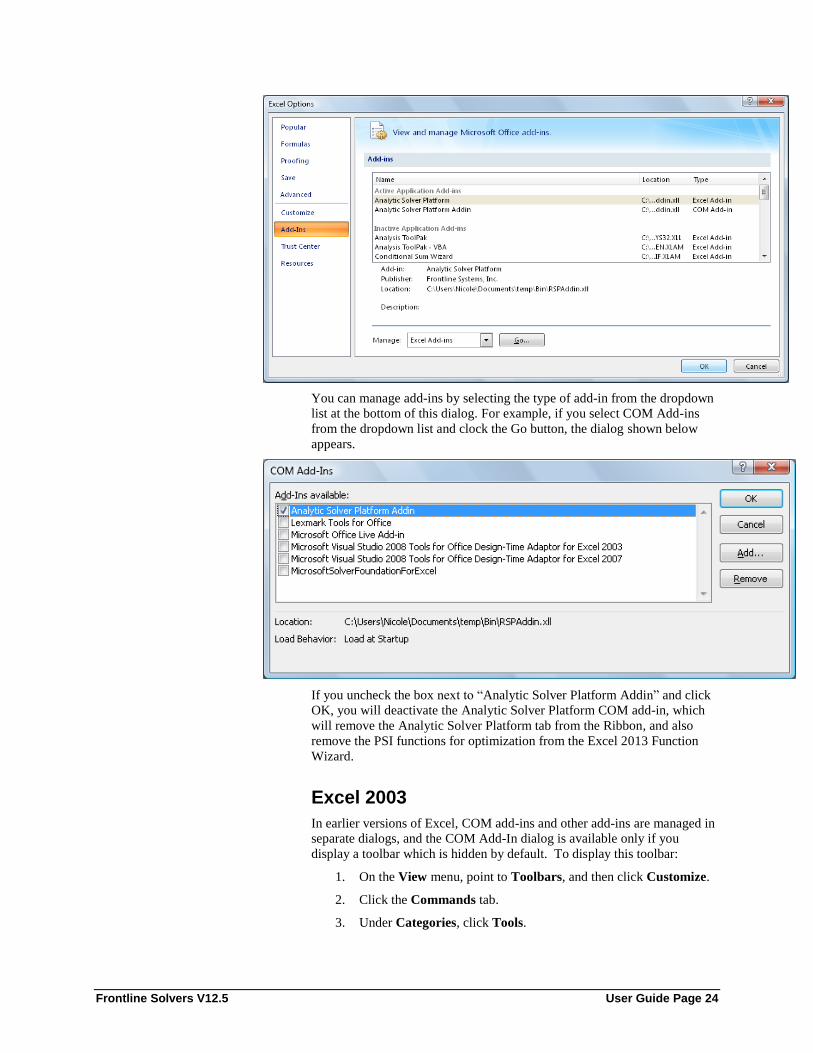
Frontline Solvers V12.5 User Guide Page 24
You can manage add-ins by selecting the type of add-in from the dropdown
list at the bottom of this dialog. For example, if you select COM Add-ins
from the dropdown list and clock the Go button, the dialog shown below
appears.
If you uncheck the box next to “Analytic Solver Platform Addin” and click
OK, you will deactivate the Analytic Solver Platform COM add-in, which
will remove the Analytic Solver Platform tab from the Ribbon, and also
remove the PSI functions for optimization from the Excel 2013 Function
Wizard.
Excel 2003
In earlier versions of Excel, COM add-ins and other add-ins are managed in
separate dialogs, and the COM Add-In dialog is available only if you
display a toolbar which is hidden by default. To display this toolbar:
1. On the View menu, point to Toolbars, and then click Customize.
2. Click the Commands tab.
3. Under Categories, click Tools.

Frontline Solvers V12.5 User Guide Page 25
4. Under Commands, click COM Add-Ins and drag your selection
to the toolbar.
Once you have done this, you can click COM Add-Ins on the toolbar to see
a list of the available add-ins in the COM Add-Ins dialog box, as shown
above.
If you uncheck the box next to “Analytic Solver Platform Addin” and click
OK, you will deactivate the Analytic Solver Platform COM add-in, which
will remove Analytic Solver Platform from the main menu bar, and also
remove the PSI functions for optimization from the Insert Function dialog.

Frontline Solvers V12.5 User Guide Page 26
Using Help, Licensing and Product Subsets
Introduction This chapter describes the ways Analytic Solver Platform V12.5 differs
from its predecessors in terms of overall operation, including registration,
licensing, use of product subsets, and use of the Startup Screen, online Help
and examples.
Working with Licenses in V12.5 A license is a grant of rights, from Frontline Systems to you, to use our
software in specified ways. Information about a license – for example, its
temporary vs. permanent status and its expiration date – is encoded in a
license code. The same binary files are used for Analytic Solver Platform
and XLMiner. The product features you see depend on the license code you
have.
Using the License File Solver.lic
Analytic Solver Platform V12.5 stores license codes in a text file named
Solver.lic. If upgrading from V12.0, no new license code will be required.
Old license codes for V11.x and earlier have no negative effect in V12.5;
they can appear in the Solver.lic file and will be ignored.
If you already have a Solver.lic file, SolverSetup adds license codes to this
file. If not, SolverSetup creates this file in a default location:
Excel 2013, 2010, 2007 or Vista: C:\ProgramData\Frontline Systems
XP: C:\Documents and Settings\All Users\Application Data\Frontline
Systems
In V12.5, V12, V11.x and V10.x, the SolverSetup program creates an
environment variable FRONTLIC whose value is the path to the Solver.lic
file. The old license manager in V9.x and earlier versions used the
environment variable LSERVRC.
License Codes and Internet Activation
You can enter a new license code at any time while you’re using Analytic
Solver Platform. To do this, choose Help – License Code from the
Analytic Solver Platform Ribbon. A dialog like the one below will appear.

Frontline Solvers V12.5 User Guide Page 27
You have two options to obtain and activate a license, using this dialog:
1. If you contact Frontline Systems at (775) 831-0300 or
[email protected], and give us the Lock Code shown in the middle of
the dialog (click the Email Lock Code button to do this quickly), we
can generate a license code for your PC, and email this to you. You
can then select and copy (Ctrl+C) the license code, and paste it
(Ctrl+V) into the lower edit box in this dialog.
2. Even easier, and available 24x7 if you have Internet access on this PC:
If you have a license Activation Code from Frontline Systems, you can
copy and paste it into the upper edit box in this dialog. When you
click OK, Analytic Solver Platform contacts Frontline’s license server
over the Internet, sends the Lock Code and receives your license code
automatically. You’ll see a message confirming the license activation,
or reporting any errors.
If you have questions, please contact Frontline Systems at (775) 831-0300
Running Subset Products in V12.5 New users often wish to download and evaluate our products for Excel. To
accommodate this, we make available downloads of the SolverSetup
program with a 15-day trial license, which gives users access to all of the
functionality and capacity of Analytic Solver Platform. But some users will
ultimately choose to purchase a license for a product that is a subset of
Analytic Solver Platform, such as XLMiner.
To help users confirm that a subset product will have the capabilities and
performance that they want, V12.5 has the ability to quickly switch
Analytic Solver Platform to operate as a subset product, without the need to
install a new license code. To do this, choose Help – Change Product on

Frontline Solvers V12.5 User Guide Page 28
the Analytic Solver Platform Ribbon. A dialog like the one below will
appear.
In this dialog, you can select the subset product you want, and click OK.
The change to a new product takes effect immediately: You’ll see the
subset product name instead of Analytic Solver Platform as a tab on the
Ribbon, and a subset of the Ribbon options
XLMiner
XLMiner includes only the data mining and predictive capabilities of
Analytic Solver Platform. No optimization or simulation capabilities are
included in the XLMiner subset.

Frontline Solvers V12.5 User Guide Page 29
Using the Welcome Screen
This screen appears automatically only when you click the Analytic Solver
Platform tab on the Ribbon in Excel 2013, 2010 or 2007, or use the
Analytic Solver Platform menu in Excel 2003 – and then only if you are
using a trial license. You can display the Welcome Screen manually by
choosing Help – Welcome Screen from the Analytic Solver Platform
Ribbon. You can control whether the screen appears automatically by
selecting or clearing the check box in the lower left corner, “Show this
dialog at first use.”
Using the XLMiner Help Text Click Help – Help Text on the XLMiner ribbon to open the Help text file.

Frontline Solvers V12.5 User Guide Page 30
This Help file contains significant information about the features and
capabilities of XLMiner – all at the tip of your fingertips. Each topic
covered includes an Introduction to the feature, an explanation of the
dialogs involved and an example using one of the example datasets. These
example datasets can be found on the XLMiner Ribbon under HELP –
Examples.

Frontline Solvers V12.5 User Guide Page 31

Frontline Solvers V12.5 User Guide Page 32
Introduction to XLMiner
Introduction
XLMiner™ is a comprehensive data mining add-in for Excel. Data mining
is a discovery-driven data analysis technology used for identifying patterns
and relationships in data sets. With overwhelming amounts of data now
available from transaction systems and external data sources, organizations
are presented with increasing opportunities to understand their data and gain
insights into it. Data mining is still an emerging field, and is a convergence
of fields like statistics, machine learning, and artificial intelligence.
Often, there may be more than one approach to a problem. XLMiner is a
tool belt to help you get started quickly offering a variety of methods to
analyze your data. It has extensive coverage of statistical and machine
learning techniques for classification, prediction, affinity analysis and data
exploration and reduction.
Ribbon Overview
To bring up the XLMiner ribbon, click XLMiner on the Excel ribbon.
The XLMiner ribbon is divided into 4 sections: Data Analysis, Time
Series, Data Mining, and Tools.
Data Analysis – This section includes four icons: Sample,
Explore, Transform, and Cluster. Click Sample to either sample
from the worksheet or a database. Click Explore to create and
manage charts. Click Transform to transform datasets with
missing date, perform binning, and to transform categorical data.
Click the Cluster Icon to perform cluster analysis.
Time Series – This section includes three icons: Partition,
ARIMA, and Smoothing and are used when analyzing a time
series.
Data Mining – This section includes four icons: Partition,
Classify, Predict, and Associate and are used to perform data
mining activities.
Tools – This section includes two icons: Score and Help. Click the
Score icon to score your test data. Click the Help icon to open

Frontline Solvers V12.5 User Guide Page 33
sample datasets, open the Help File, and check for updates. See
below for a complete discussion of the Help icon.
Click the XLMiner menu item in Excel 2003 to open the XLMiner menu.
This menu is arranged a bit differently than the Excel 2007 / 2010 / 2013
ribbon, but all features discussed in this guide can be used in Excel 2003.
Note: Menu items appear differently in Excel 2003 but all method dialogs
are identical to dialogs in later versions of Excel.
XLMiner Help Ribbon Icon To open XLMiner Help, simply click the Help icon on the XLMiner ribbon.
Here you will be able to change the product that you are using (Analytic
Solver Platform or a subset such as XLMiner), obtain your lock code and
enter your permanent license, open example datasets, search the online help
text, and check for updates.
Change Product Selecting Change Product on the XLMiner Help menu will bring up the
Change Product dialog shown below.

Frontline Solvers V12.5 User Guide Page 34
If you have a permanent license code for the Analytic Solver Platform, then
you can change to any subset and see that subset on the Ribbon. For
example, if XLMiner is selected, only XLMiner will appear on the ribbon
even if a license for Analytic Solver Platform is in place.
License Code Selecting License Code from the XLMiner Help menu brings up the Enter
License or Activation Code dialog shown below. The top portion of this
dialog will always contain the currently licensed product along with the
product version number.
To obtain your permanent license, contact Frontline Systems by phone
(888-831-0333) or email ([email protected]) to obtain an activation code.

Frontline Solvers V12.5 User Guide Page 35
Enter the activation code into the Activation Code field leaving the License
Code field blank. Then click OK. At this point, your permanent license
should be activated and no further steps are needed.
If you encounter problems connecting to our license server, then you will
need to enter the complete license directly into this dialog. Clicking Email
Lock Code will create and send an email to [email protected] that includes
the Lock Code displayed on this dialog. Our license manager will generate
a license based on this lock code and email the permanent license code back
to you. (Make sure to click Allow on the dialog below.)
Copy and paste the entire contents of the license code into the License Code
field as shown on the dialog below, then click OK. At this point, your
permanent license should be activated and no further steps are needed.

Frontline Solvers V12.5 User Guide Page 36
Examples
Clicking this menu item will open a browser pointing to C:\Program
Files\Frontline Systems\ Analytic Solver Platform \Datasets. See the table
below for a description of each example dataset.
Model Used in Example Notes
Airpass Time Series
The classic Box & Jenkins airline dataset. Monthly totals of international airline passengers (1949 - 1960)
All Temperature
Temperature dataset.
Apparel
Apparel sales from Jan 1988 to Dec 2001.
Arma
Monthly stereo sales from Jan 1988 to Dec 1998.
Associations Association Rules
This dataset is a subset of the Charles Book Club dataset and is used in the Association Rules example.

Frontline Solvers V12.5 User Guide Page 37
AssociationsItemList
This dataset can be used with the Association Rules method.
Binning Example Bin Continuous Data Example dataset used in the Bin Continuous Data example
Boston Housing
Scoring Test Data, Matrix Plots, Histrogram, Classification Tree,
Regression Tree, K-Nearest Neighbors Prediction, Neural Networks Classification, Multiple Linear
Regression, Discriminant Analysis
This dataset contains data collected in 1970 by the U.S. Census Service concerning housing in the Boston, MA area.
Boxplot Box Plot This example dataset is used in the Box Plot example.
Catalog Multi Partition with Oversampling
This dataset contains a response to a direct mail offer, published by DMEF, the Direct Marketing Educational Foundation, and is used in the Partition with Oversampling example.
Charles Book Club Scoring Test Data, Logistic Regression This dataset derived for The Bookbinders Club, a Case Study in Database Marketing.
Daily Rate
Daily Rate information for years 1955 - 2001.
Dataset.mdb
A synthetic database that includes Boston_Housing, Charles_BookClub, Digits, Flying_Fitness, Iris, Utilities, and Wine datasets.
Demo.mdb
A synthetic database.
Digits Discriminant Analysis
This dataset was used in the book CART by Leo Breiman et. al. and is used in several XLMiner examples.
DistMatrix Hierarchical Clustering This dataset is used in the Hierarchical Clustering example.
Durable Goods
Monthly sales figures for years 1988 – 2001
Examples Missing Data Handling This dataset is used in the Missing Data Handling example
Flying Fitness Discriminant Analysis & Naïve Bayes This dataset includes test results of flying fitness tests for 40 pilots (var 1).
Income Time Series This dataset is used in the Time Series Example
Iris k-Nearest Neighbors Classification
This dataset was introduced by R. A. Fisher and reports four characteristics of three species of iris flower.
Irisfacto Transform Categorical Data This dataset is a subset of the Iris dataset.

Frontline Solvers V12.5 User Guide Page 38
Monthly Rate
This dataset includes monthly rate information for years 1949 – 2001.
Retail Trade
This dataset includes retail sales data for years 1988 – 2001.
Sampling Sampling from Worksheet This dataset is used in the Sampling from Worksheet example.
Scoring Scoring Test Data This dataset is used in the Scoring Test Data example.
Universal Bank Database
This synthetic database was created to test Predictive Modeling.
Universal Bank Main
This synthetic dataset was created to test Predictive Modeling.
Utilities Principal Components Analysis &
Hierarchical Clustering
This dataset gives corporate data on 22 US public utilities and can be found in Dean W. Wichern’s & Richard Arnold Johnson’s Applied Multivariate Statistical Analysis, Prentice Hall, 5th Ed (2002).
Wine
Discriminant Analysis, K-Means Clustering, Manual and Automatic
Neural Networks Classification, Standard Data Partition
The wine dataset contains properties of wine taken from three different wineries in the same region. This dataset can be found in the UCI Machine Learning Repository.
Wine Partition Standard Data Partition This example file is used in the Standard Data Partition example.
Help Text Clicking Help Text opens the online Help file. This file contains extensive
information pertaining to XLMiner’s features and capabilities. All at the tip
of your fingertips!

Frontline Solvers V12.5 User Guide Page 39
Check for Updates Analytic Solver Platform will confirm that the latest version is installed
when this menu item is selected. If not, you will be instructed to visit our
Website at www.solver.com to download the latest version.
About XLMiner
Clicking this menu item will open the About XLMiner dialog as shown
below.

Frontline Solvers V12.5 User Guide Page 40
Common Dialog Options These options, fields, and command buttons appear on most XLMiner
dialogs.
Worksheet
The active worksheet appears in this field
Data Range
The range of the dataset appears in this field
# Rows, # Columns
The number of rows and columns in the dataset appear in these two fields,
respectively.

Frontline Solvers V12.5 User Guide Page 41
First row contains headers
If this option is selected, variables will be listed according to the first row in
the dataset.
Variables in the data source
All variables contained in the dataset will be listed in this field.
Input variables
Variables listed in this field will be included in the output. Select the
desired Variables in the data source then click the > button to shift
variables to the Input variables field.
Help
Click this command button to open the XLMiner Help text file.
Reset
Click this command button to reset the options for the selected method.
OK
Click this command button to initiate the desired method and produce the
output report.
Cancel
Click this command button to close the open dialog without saving any
options or creating an output report.

Frontline Solvers V12.5 User Guide Page 42
Help Window
Click this command button to open the Help Text for the selected method.
References See below for a list of references sited when compiling this guide.
Websites
1. The Data & Analysis Center for Software. <https://www.thecsiac.com>
2. NEC Research Institute Research Index: The NECI Scientific Literature
Digital Library.
<http://www.iicm.tugraz.at/thesis/cguetl_diss/literatur/Kapitel02/URL/NEC
/cs.html>.
3. Thearling, Kurt. Data Mining and Analytic Technologies.
<http://www.thearling.com>
Books
1. Anderberg, Michael R. Cluster Analysis for Applications. Academic Press
(1973).
2. Berry, Michael J. A., Gordon S. Linoff. Mastering Data Mining. Wiley
(2000).
3. Breiman, Leo Jerome H. Friedman, Richard A. Olshen, Charles J. Stone.
Classification and Regression Trees. Chapman & Hall/CRC (1998).
4. Han, Jiawei, Micheline Kamber. Data Mining: Concepts and Techniques.
Morgan Kaufmann Publishers (2000).
5. Hand, David, Heikki Mannila, Padhraic Smyth. Principles of Data Mining.
MIT Press, Cambridge (2001).
6. Hastie, Trevor, Robert Tibshirani, Jerome Friedman. The Elements of
Statistical Learning: Data Mining, Inference, and Prediction. Springer, New
York (2001).
7. Shmueli, Galit, Nitin R. Patel, Peter C. Bruce. Data Mining for Business
Intelligence. Wiley, New Jersey (2010).

Frontline Solvers V12.5 User Guide Page 43
Sampling from a Worksheet or Database
Introduction A statistician often comes across huge volumes of information from which he or
she wants to draw inferences. Since time and cost limitations make it impossible
to go through every entry in these enormous datasets, statisticians must resort to
sampling techniques. These sampling techniques choose a reduced sample or
subset from the complete dataset. The statistician can then perform his or her
statistical procedures on this reduced dataset saving much time and money.
Let’s review a few statistical terms. The entire dataset is called the population.
A sample is the portion of the population that is actually examined. A good
sample should be a true representation of the population to avoid forming
misleading conclusions. Various methods and techniques have been developed
to ensure a representative sample is chosen from the population. A few are
discussed here.
Simple Random Sampling This is probably the simplest method for
obtaining a good sample. A simple random sample of say, size n, is
chosen from the population in such a way that every random set of n
items from the population has an equal chance of being chosen to be
included in the sample. Thus simple random sampling not only avoids
bias in the choice of individual item but also gives every possible
sample an equal chance.
The Data Sampling utility of XLMiner offers the user the freedom to
choose sample size, seed for randomization, and sampling with or
without replacement.
Stratified Random Sampling In this technique, the population is first
divided into groups of similar items. These groups are called strata.
Each stratum, in turn, is sampled using simple random sampling. These
samples are then combined to form a stratified random sample.
The Data Sampling utility of XLMiner offers the user the freedom to
choose a sorting seed for randomization and sampling with or without
replacement. The desired sample size can be prefixed by the user
depending on which method is being chosen for stratified random
sampling.
XLMiner allows sampling either from a worksheet or a database.

Frontline Solvers V12.5 User Guide Page 44
Sampling from a Worksheet Below are three examples that illustrate how to perform Simple Random
Sampling with and without replacement and Stratified Random Sampling from a
worksheet.
Example: Sampling from a Worksheet using Simple Random Sampling
Open the dataset Sampling.xlsx by clicking Help – Examples (Excel 2003:
Open Data – Example Files) from the XLMiner ribbon. This dataset contains a
variable ID for the record identification and seven variables, v1, v2, v7, v8, v9,
v10, v11.
To start, click a cell within the data, say A2, and click Data Utilities -- Sample
from Worksheet.

Frontline Solvers V12.5 User Guide Page 45
In this example, the default option, Simple Random Sampling, will be used.
Select all variables under Variables, click >_ to include them in the sample data
then click OK.

Frontline Solvers V12.5 User Guide Page 46
A portion of the output is shown below.

Frontline Solvers V12.5 User Guide Page 47
The output is a simple random sample without replacement, with a default
random seed setting of 12345. The desired sample size is 87 records as shown
above. Note that XLMiner has introduced one more variable, Row ID in the
sample. Every dataset may not have a number allocated to each record. The
variable, Row ID gives IDs to records before sampling, and then sorts the output
on those IDs before producing the output. Row ID proves handy when the user
wishes to go back to the dataset for crosschecking information.
Example: Sampling from a Worksheet using Sampling with Replacement
Click the data tab on the Sampling.xlsx worksheet and again click a cell within
the data, say A2, then click Data Utilities -- Sample from Worksheet to bring
up the Sampling dialog.
Again, select all variables in the Variables section and click >_ to include each
in the sample data. Check Sample with replacement and enter 300 for Desired
sample size. Since we are choosing sampling with replacement, XLMiner will
generate a sample with a larger number of records than the dataset. Click OK.
A portion of the output is shown below.

Frontline Solvers V12.5 User Guide Page 48
The output indicates "True" for Sampling with replacement. As a result, the
desired sample size is greater than the number of records in the input data.
Looking closely, one can see that the second and third entries are the same
record, record #3.
Example: Sampling from a Worksheet using Stratified Random Sampling
Click the data worksheet, click a cell within the data, say A2, and click Data
Utilities -- Sample from Worksheet.
Select all variables under Variables, click >_ to include them in the sample data,
and then click OK. Enter 100 for Desired sample size and 45689 for Set seed.
Select Stratified random sampling.
Click the down arrow next to Stratum Variable and select v8 (XLMiner allows
only those variables which have less than 30 distinct values.) The strata number
is automatically displayed once you select v8. Select Proportionate to stratum
size. Then click OK.

Frontline Solvers V12.5 User Guide Page 49

Frontline Solvers V12.5 User Guide Page 50
In order to maintain the proportions of the strata, XLMiner has increased the
sample size. This is apparent in the entry for #records actually sampled. Under
the Stratum wise details heading, XLMiner has listed all the stratum values v8
assumes with #records in input data for each stratum. On this basis, XLMiner
calculated the percentage representation of that value in the dataset and
maintained it in the sample. This is evident in the entries since #records in
sampled data has the same proportion as in the dataset. XLMiner has added a
Row Id to each record before sampling. The output is displayed after sorting the
sample on these Row Ids.
Let’s see what happens to our output when we select a different option for
Stratified Sampling.
Click back to the data worksheet, click a cell within the data, say A2, and click
Data Utilities -- Sample from Worksheet.
Select all variables under Variables, click >_ to include them in the sample data,
and then click OK. Select Stratified random sampling. Choose v8 as the
Stratum variable. The #strata is displayed automatically. Select Equal from
each stratum, please specify #records.
Enter the #records. Remember, this number should not be greater than the
smallest stratum size. In this case the smallest stratum size is 8. (Note: The
smallest stratum size appears automatically in a box next to the option, Equal
from each stratum, # records = smallest stratum size.). Enter 7, which is less
than the limit of 8, and then click OK.

Frontline Solvers V12.5 User Guide Page 51
As you can see in the output, the number of records in the sampled data is 56 or
7 records per stratum for 8 strata.
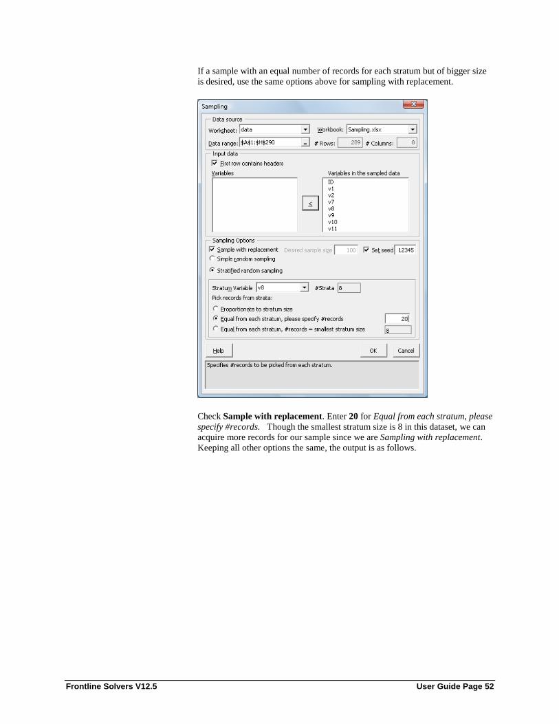
Frontline Solvers V12.5 User Guide Page 52
If a sample with an equal number of records for each stratum but of bigger size
is desired, use the same options above for sampling with replacement.
Check Sample with replacement. Enter 20 for Equal from each stratum, please
specify #records. Though the smallest stratum size is 8 in this dataset, we can
acquire more records for our sample since we are Sampling with replacement.
Keeping all other options the same, the output is as follows.

Frontline Solvers V12.5 User Guide Page 53
Since the output sample has 20 records per stratum, the #records in sampled
data is 160 (20 records per stratum for 8 strata).
Sample from Worksheet Options Please see below for a complete list of each option contained on the Sampling
from Worksheet dialog.

Frontline Solvers V12.5 User Guide Page 54
Data Range
Either type the address directly into this field, or use the reference button, to
enter the data range from the worksheet. If the cell pointer (active cell) is
already somewhere in the data range, XLMiner automatically picks up the
contiguous data range surrounding the active cell. After the data range is
selected, XLMiner displays the number of records in the selected range.
First row contains headers
When this box is checked, XLMiner picks up the headings from the first row of
the selected data range. When the box is unchecked, XLMiner follows the
default naming convention, i.e., the variable in the first column of the selected
range will be called "Var1", the second column "Var2," etc.
Variables
This list box contains the names of the variables in the selected data range. If the
first row of the range contains the variable names, then these names appear in
this list box. If the first row of the dataset does not contain the headers, then
XLMiner lists the variable names using its default naming convention. In this
case the first column is named Var1; the second column is named Var2 and so
on. To select a variable for sampling, select the variable, then click the ">"
button. Use the CTRL key to select multiple variables.

Frontline Solvers V12.5 User Guide Page 55
Sample With replacement
If this option is checked the data will be sampled with replacement. The default
is sampling without replacement.
Set Seed
Enter the desired sorting seed here. The default seed is 12345.
Desired sample size
Enter the desired sample size here. (Note that the actual sample size in the
output may vary a little, depending on additional options selected.)
Simple random sampling
The data is sorted using the simple random sampling technique, taking into
account the additional parameter settings.
Stratified random sampling
If selected, XLMiner enables the following additional options.
Stratum Variable
Select the variable to be used for stratified random sampling by clicking the
down arrow and selecting the desired variable. Note that XLMiner allows only
those variables which have less than 30 distinct values. As the user selects the
variable name, XLMiner displays the #Strata that variable contains in a box to
the left and the smallest stratum size in a box in front of the option Equal from
each stratum, #records = smallest stratum size.
Proportionate to stratum size
XLMiner detects the proportion of each stratum in the dataset and maintains the
same in sampling. Due to this, XLMiner sometimes must increase the sample
size in order to maintain the proportionate stratum size. XLMiner then displays
the actual sample size in the output along with the desired sample size.
Equal from each stratum
On specifying the number of records, XLMiner generates a sample which has
the same number of records from each stratum. In this case the number chosen
automatically decides the desired sample size. As a result, the option to enter
the desired sample size is disabled.

Frontline Solvers V12.5 User Guide Page 56
Equal from each stratum, #records = smallest stratum size
XLMiner detects the smallest stratum size and generates a sample wherein every
stratum has a representation of that size. Again, the option for the desired
sample size is disabled.
XLMiner performs the stratified random sampling with or without replacement.
If Sample with replacement is not selected, the desired sample size must be less
than the number of records in the dataset.
If Sample with replacement is selected, then the number of records in the dataset
does not pose any limit on the number of records in the sample. XLMiner can
generate a sample having up to 2000 records.
Before sampling, XLMiner generates a Row ID for each record (irrespective of
whether the dataset already has one). XLMiner sorts the sampled output
according to Row ID before displaying it.
Sampling from a Database Click Data Utilities – Sample from Database on the XLMiner ribbon to display
the following dialog.
Click the down arrow next to Data Source and select MS-Access, and then click
Connect to a database.

Frontline Solvers V12.5 User Guide Page 57
Click Browse for database file… and browse to C:\Program Files\Frontline
Systems\Analytic Solver Platform\Datasets. Select the Demo.mdb Microsoft
Access database, and then click Open.
Click OK on the MS-Access database file dialog.
Since this database is not password protected, simple click OK. The following
dialog will appear.

Frontline Solvers V12.5 User Guide Page 58
Select all the fields from Fields in table and click > to move all fields to Selected
fields.
Click OK. A portion of the output is below.
Refer to the examples above for Sampling from a Worksheet. You can sample
from a database using all the methods described in this chapter.

Frontline Solvers V12.5 User Guide Page 59
Exploring Data using Charts
Introduction XLMiner offers eight different types of charts to visually explore your data: Bar
Charts, Line Charts, ScatterPlots, Boxplots, Histograms, Parallel Coordinates,
ScatterPlot Matrices and Variable Plots. To create a chart, invoke the Chart
Wizard by clicking Explore on the XLMiner ribbon. A description of each chart
type follows.
Bar Chart
The bar chart is one of the easiest and effective plots to create and understand.
The best application for this type of chart is comparing an individual statistic
(i.e. mean, count, etc.) across a group of variables. The bar height represents the
statistic while the bars represent the different groups. An example of a bar chart
is shown below.
Box Whisker Plot
A box plot graph summarizes a dataset and is often used in exploratory data
analysis. This type of graph illustrates the shape of the distribution, its central
value, and the range of the data. The plot consists of the most extreme values in
the data set (maximum and minimum values), the lower and upper quartiles, and
the median.
Box plots are also very useful when large numbers of observations are involved
or when two or more data sets are being compared. In addition, they are also
helpful for indicating whether a distribution is skewed and whether there are any
unusual observations (outliers) in the data set. The most important trait of the
box plot is its failure to be strongly influenced extreme values, or outliers.
Let’s review the following statistical terms below.

Frontline Solvers V12.5 User Guide Page 60
Median: The median value in a dataset is the value that appears in the middle of
a sorted dataset. If the dataset has an even number of values then the median is
the average of the two middle values in the dataset.
Quartiles: Quartiles, by definition, separate a quarter of data points from the
rest. This roughly means that the first quartile is the value under which 25% of
the data lie and the third quartile is the value over which 25% of the data are
found. (Note: This indicates that the second quartile is the median itself.)
First Quartile, Q1: Concluding from the definitions above, the first quartile is
the median of the lower half of the data. If the number of data points is odd, the
lower half includes the median.
Third Quartile, Q3: Third quartile is the median of the upper half of the data. If
the number of data points is odd, the upper half of the data includes the median.
See the following example.
Consider the following dataset --
52, 57, 60, 63, 71, 72, 73, 76, 98, 110, 120
The dataset has 11 values sorted in ascending order. The median is the middle
value, (i.e. 6th value in this case.)
Median = 72
Q1 is the median of the first 6 values, (i.e. the mean of 3rd and 4th values)
25th
Percentile = 61.5
Q3 is the median of the last 6 values. (i.e. the mean of the 8th
and 9th
values).
75th
Percentile = 87
The mean is the average of all the data values ((52 + 57 + 60 + 63 + 71 + 72 +
73 + 76 + 98 + 110 + 120) / 11).
Mean = 77.45
Interquartile Range = 25.5 The Interquartile range is a useful measure of the
amount of variation in a set of data and is simply the 75th
Percentile – 25th
Percentile (87 – 61.5 = 25.5)
The box extends from Q1 to Q3 and includes Q2. The extreme points are
included the "whiskers". This means the box includes the middle one- half of the
data. In XLMiner, the mean is denoted with a dotted line and the median with a
solid line. XLMiner completes the box plot by extending its "whiskers" to the
most extreme points, 52 and 120.
Max: 120
Min: 52

Frontline Solvers V12.5 User Guide Page 61
Histogram
A Histogram, or a Frequency Histogram is a bar graph which depicts the range
and scale of the observations on the x axis and the number of data points (or
frequency) of the various intervals on the y axis. These types of graphs are
popular among statisticians. Although these types of graphs do not show the
exact values of the data points, they give a very good idea about the spread and
shape of the data.
Consider the percentages below from a college final exam.
82.5, 78.3, 76.2, 81.2, 72.3, 73.2, 76.3, 77.3, 78.2, 78.5, 75.6, 79.2, 78.3, 80.2,
76.4, 77.9, 75.8, 76.5, 77.3, 78.2
One can immediately see the value of a histogram by taking a quick glance at
the graph below. This plot quickly and efficiently illustrates the shape and size
of the dataset above. Note: XLMiner determines the number and size of the
intervals when drawing the histogram.
Line Chart
A line chart is best suited for time series datasets. In the example below, the line
chart plots the number of airline passengers from January 1949 to December
1960. (The X – axis is the number of months starting with January 1949 as “1”.)

Frontline Solvers V12.5 User Guide Page 62
Parallel Coordinates
A Parallel Coordinates plot consists of N number of vertical axes where N is the
number of variables selected to be included in the plot. A line is drawn
connecting the observation’s values for each different variable (each different
axis) creating a “multivariate profile”. These types of graphs can be useful for
prediction and possible data binning. In addition, these graphs can expose
clusters, outliers and variable “overlap”. Axes can be reordered by simply
dragging and axis and moving the axis to the desired location. . An example of
a Parallel Coordinates plot is shown below.
Scatterplot
One of the most common, effective and easy to create plots is the scatterplot.
These graphs are used to compare the relationships between two variables and
are useful in identifying clusters and variable “overlap”.

Frontline Solvers V12.5 User Guide Page 63
Scatterplot Matrix
A Matrix plot combines several scatterplots into one panel enabling the user to
see pairwise relationships between variables. Given a set of variables Var1,
Var2, Var3, ...., Var N the matrix plot contains all the pairwise scatter plots of
the variables on a single page in a matrix format. The names of the variables are
on the diagonals. In other words, if there are k variables, there will be k rows
and k columns in the matrix and the ith row and jth column will be the plot of
Vari versus Varj.
The axes titles and the values of the variables appear at the edge of the
respective row or column. The comparison of the variables and their interactions
with one another can be studied easily and with a simple glance which is why
matrix plots are becoming increasingly common in general purpose statistical
software programs. An example is shown below.
Variable Plot
XLMiner’s Variables graph simply plots each selected variable’s distribution.
See below for an example.

Frontline Solvers V12.5 User Guide Page 64
Bar Chart Example This example describes the use of the Bar Chart to illustrate the details of the
Boston_Housing.xlsx dataset.
Click Help – Examples on the XLMiner ribbon to open the
Boston_Housing.xlsx example file.
Select a cell within the data (say A2), then click Explore – Chart Wizard to
bring up the first dialog of the Chart Wizard.
Click Next.
On the Y Axis Selection Dialog, select MEDV, and then click Next.

Frontline Solvers V12.5 User Guide Page 65
Select CHAS on the X-Axis Selection dialog, then click Finish. Click Next to
set Panel and Color options. These options can always be set in the upper right
hand corner of the plot.
Click the right pointing arrow next to Count of MEDV and select MEDV from
the menu. When the second menu appears (below the first selection of MEDV)
select Mean.

Frontline Solvers V12.5 User Guide Page 66
The Y axis changes to Mean of MEDV.
This y-axis variable, Mean of MEDV (Median value of owner-occupied homes)
is a numerical variable and the CHAS variable is a categorical variable. The
two bars represent homes in the Boston area that are located close to the Charles
River (1) and homes that are not (0). The first bar (0 bar) shows the average of
the median value of owner occupied homes that are not located close to the
Charles River. The second bar (1 bar) shows the average of the median value of
owner occupied homes that are located close to the Charles River. We can
conclude from this graph that homes located next to the Charles River are more
expensive than homes that are not located next to the Charles River.

Frontline Solvers V12.5 User Guide Page 67
Click the right pointing arrow next to Mean of MEDV and select CAT.MEDV
from the first menu. When the second menu appears (below the first selection
of CAT.MEDV) select Percentage.
This bar chart includes a categorical variable, CAT. MEDV, on the y-axis. This
variable is a 0 if MEDV is less than 30 (MEDV < 30), otherwise the variable
value is a 1. A user can quickly see that the majority of houses are located far
away from the Charles River.
Uncheck the 1 under the CHAS filter to view only homes located far away from
the Charles river.
To change the variable on the X-axis, simply click the down arrow and select
the desired variable from the menu.

Frontline Solvers V12.5 User Guide Page 68
To add a 2nd
Bar Chart simply click the Bar Chart icon at the top of the Chart
Wizard.
A second chart is added to the Chart Wizard dialog. Click the X in the upper
right corner of each plot to remove from the window. Color by and Panel by
options are always available in the upper right hand corner of each plot.
The top graph shows the count of all records in each category. Since each
category includes the same amount of observations, all bars are set to the same
height.
Please see the Common Chart Options section (below) for a complete
description of each icon on the chart title bar.
To exit the graph, click the red X in the upper right hand corner of the Chart
Wizard window.

Frontline Solvers V12.5 User Guide Page 69
To save the chart for later viewing, click Save. To delete the chart, click
Discard, to cancel the save and return to the chart, click Cancel. For this
example, enter BarChart for the chart name, then click Save. The chart will
close. To reopen the chart, click Explore – Existing Charts – BarChart.
Box Whisker Plot Example This example describes the use of the Boxplot chart to illustrate the
characteristics of the dataset.
Click Help – Examples on the XLMiner ribbon to open the BoxPlot.xlsx
example file.
Select on a cell within the data (say A2), then click Explore – Chart Wizard to
bring up the first dialog of the Chart Wizard. Select BoxPlot, and then click
Next.
On the Y Axis Selection dialog, select Y1, and then click Next.

Frontline Solvers V12.5 User Guide Page 70
Select X-Var on the X-Axis Selection dialog, then click Finish. Click Next to
set Panel and Color options. These options can always be set in the upper right
hand corner of the plot.

Frontline Solvers V12.5 User Guide Page 71
Uncheck class 4 under the X-Var filter to remove this class from the plot.
Hover next to the plot to display the following Intellisense window.

Frontline Solvers V12.5 User Guide Page 72
The dotted line denotes the Mean of 22.49, the solid line denotes the Median of
23.22. The box reaches from the 25th
Percentile of 9.07 to the 75th
Percentile of
37.87. The lower “whisker” (or lower bound) reaches to -47.343 and the upper
“whisker” (or upper bound) reaches to 61.454.
To select a different variable on the y-axis, click the right pointing arrow and
select the desired variable from the menu.
To change the variable on the X-axis, select the down arrow next to X-Var and
select the desired variable.

Frontline Solvers V12.5 User Guide Page 73
To add a 2nd
boxplot, click the BoxPlot icon on the top of the Chart Wizard
dialog.
A second chart is added to the Chart Wizard dialog. Click the X in the upper
right corner of each plot to remove from the window. Color by and Panel by
options are always available in the upper right hand corner of each plot.
To exit the graph, click the red X in the upper right hand corner of the Chart
Wizard window.
Please see the Common Chart Options section (below) for a complete
description of each icon on the chart title bar.

Frontline Solvers V12.5 User Guide Page 74
To save the chart for later viewing, click Save. To delete the chart, click
Discard, to cancel the save and return to the chart, click Cancel. For this
example, enter BoxPlot for the chart name, then click Save. The chart will
close. To reopen the chart, click Explore – Existing Charts – BoxChart. To
delete the chart, click Discard.
Histogram Example The example below illustrates the use of XLMiner’s chart wizard in drawing a
histogram of the Boston_Housing.xlsx dataset. Click Help – Examples on the
XLMiner ribbon to open the example dataset, Boston_Housing.xlsx. Select a
cell within the dataset, say A2, and then click Explore – Chart Wizard on the
XLMiner ribbon. The following dialog appears.
Select Histogram, and then click Next.

Frontline Solvers V12.5 User Guide Page 75
Select Frequency, then click Next.
Select INDUS, then click Finish.

Frontline Solvers V12.5 User Guide Page 76
The data has been divided into 14 different bins or intervals. Unselect the
variables CRIM and ZN under Filters. Notice the graph did not change. This
is because removing these variables is, in effect, removing a column from the
dataset. Since we are currently not interested in these columns, the plot is not
affected. However, now uncheck 0 under the CHAS variable.
Notice the number of bins has been reduced to 7 (down from 13). This is
because removing the 0 class from the CHAS variable is, in effect, removing
rows from the dataset, which does affect the INDUS variable in the plot.
To change the variables included in the plot, simply click the Histogram icon on
the title bar of the Chart Wizard,

Frontline Solvers V12.5 User Guide Page 77
to bring up the X-Y Axis Selection dialog.
Select DIS for the X-Axis, then click Next to choose color and panel options.
At this point, you could also click Finish to draw the histogram. Color and
panel options can be chosen at any time.
Select CAT. MEDV for Color By, then click Finish to draw the histogram.

Frontline Solvers V12.5 User Guide Page 78
The two histograms are drawn in the same window. Click the X in the upper
right corner of each plot to remove from the window. Color by and Panel by
options are always available in the upper right hand corner of each plot.
Please see the section Common Chart Options (below) for a complete
description of each icon on the chart title bar.
To exit the graph, click the red X in the upper right hand corner of the Chart
Wizard window.
To save the chart for later viewing, click Save. To delete the chart, click
Discard, to cancel the save and return to the chart, click Cancel. For this
example, type Histogram for the chart name, then click Save. The chart will
close. To reopen the chart, click Explore – Existing Charts – Boxplot.
Line Chart Example The example below illustrates the use of XLMiner’s chart wizard in drawing a
Line Chart using the Airpass.xlsx dataset. Click Help – Examples on the
XLMiner ribbon to open the example dataset, Airpass.xlsx. Select a cell within

Frontline Solvers V12.5 User Guide Page 79
the dataset, say A2, and then click Explore – Chart Wizard on the XLMiner
ribbon. The following dialog appears.
Select Line Chart, then click Next.
Select Passengers, then click Next.

Frontline Solvers V12.5 User Guide Page 80
Select Observation#, then select Finish. Click Next to choose Panel and Color
options. Both can be selected or changed in the upper right hand corner of the
plot.
The y-axis plots the number of passengers and the x-axis plots the month
number (starting with 1 for January 1949). The plot shows that as the months
progress, the number of airline passengers increases.
Please see the section Common Chart Options (below) for a complete
description of each icon on the chart title bar.
To exit the graph, click the red X in the upper right hand corner of the Chart
Wizard window.

Frontline Solvers V12.5 User Guide Page 81
To save the chart for later viewing, click Save. To delete the chart, click
Discard, to cancel the save and return to the chart, click Cancel. For this
example, type LineChart for the chart name, then click Save. The chart will
close. To reopen the chart, click Explore – Existing Charts – LineChart.
Parallel Coordinates Chart Example The example below illustrates the use of XLMiner’s chart wizard in drawing a
Parallel Coordinates Plot using the Boston_Housing.xlsx dataset. Click Help –
Examples on the XLMiner ribbon to open the example dataset,
Boston_Housing.xlsx. Select a cell within the dataset, say A2, then click
Explore – Chart Wizard on the XLMiner ribbon. The following dialog
appears.
Select Parallel Coordinates, then click Next.

Frontline Solvers V12.5 User Guide Page 82
Select all variables except MEDV. (The CAT.MEDV variable is used in place
of the MEDV variable. CAT.MEDV is a categorical variable where a 1 denotes a
MEDV value larger than 30.)
Click Finish to draw the plot.
Uncheck the class 1 value for the CAT. MEDV variable.

Frontline Solvers V12.5 User Guide Page 83
Leaving the Chart Wizard window open, click back to the Data worksheet
(within the Boston_Housing workbook), then click Explore – Chart Wizard to
open a 2nd
instance of the Chart Wizard. Select Parallel Coordinates on the
first Chart Wizard dialog and then select all variables except MEDV on the
Variable Selection dialog. When the 2nd
plot is drawn, unselect the 0 class for
the CAT.MEDV variable.

Frontline Solvers V12.5 User Guide Page 84
The first characteristic that is evident is that there are more houses with a value
of 0 for CAT. MEDV (Median value of owner-occupied homes < 30,000) than
with a value of 1 (Median value of owner-occupied homes > 30,000). In
addition, the more expensive houses (CAT.MEDV = 1) have lower CRIM (Per
capita crime rate by town) and LSAT (% Lower status of the population) values
and higher RM (Average number of rooms per dwelling) values.
Select the “0” CAT. MEDV chart and select “1” under CAT. MEDV. Then
select CAT.MEDV for Color By. The chart now displays both classes of
CAT.MEDV (0 and 1) on the same chart. However, each class is given a
different color, blue for “0” and yellow for “1”.

Frontline Solvers V12.5 User Guide Page 85
To remove a variable from the matrix, unselect the desired variable under
Filters. To add a variable to the matrix, select the desired variable under Filters.
Please see the section Common Chart Options (below) for a complete
description of each icon on the chart title bar.
To exit the graph, click the red X in the upper right hand corner of the Chart
Wizard window.
To save the chart for later viewing, click Save. To delete the chart, click
Discard, to cancel the save and return to the chart, click Cancel. For this
example, type Parallel for the chart name, then click Save. The chart will close.
To reopen the chart, click Explore – Existing Charts – Parallel.
ScatterPlot Example The example below illustrates the use of XLMiner’s chart wizard in drawing a
Scatterplot using the Boston_Housing.xlsx dataset. Click Help – Examples on
the XLMiner ribbon to open the example dataset, Boston_Housing.xlsx. Select

Frontline Solvers V12.5 User Guide Page 86
a cell within the dataset, say A2, and then click Explore – Chart Wizard on the
XLMiner ribbon. The following dialog appears.
Select ScatterPlot, then click Next.
Select LSTAT on the Y Axis Selection Dialog.

Frontline Solvers V12.5 User Guide Page 87
Select MEDV from the X-Axis Selection Dialog. Then click Finish.
Select Color by: CHAS (Charles River dummy variable = 1 if tract bounds
river; 0 otherwise) and Panel by: CAT.MEDV (Median value of owner-
occupied homes in $1000's > 30).
This new graph illustrates that most houses that border the river are higher
priced homes.

Frontline Solvers V12.5 User Guide Page 88
To remove a variable from the matrix, unselect the desired variable under
Filters. To add a variable to the matrix, select the desired variable under Filters.
Please see the section Common Chart Options (below) for a complete
description of each icon on the chart title bar.
To exit the graph, click the red X in the upper right hand corner of the Chart
Wizard window.
To save the chart for later viewing, click Save. To delete the chart, click
Discard, to cancel the save and return to the chart, click Cancel. For this

Frontline Solvers V12.5 User Guide Page 89
example, type Scatterplot for the chart name, then click Save. The chart will
close. To reopen the chart, click Explore – Existing Charts – Scatterplot.
Scatterplot Matrix Plot Example The example below illustrates the use of XLMiner’s chart wizard in drawing a
Scatterplot Matrix using the Boston_Housing.xlsx dataset. Click Help –
Examples on the XLMiner ribbon to open the example dataset,
Boston_Housing.xlsx. Select a cell within the dataset, say A2, then click
Explore – Chart Wizard on the XLMiner ribbon. The following dialog
appears.
Select Scatterplot Matrix, then click Next.
Select INDUS, AGE, DIS, and RAD variables, then click Finish.

Frontline Solvers V12.5 User Guide Page 90
Histograms of the selected variables appear on the diagonal. Find the plot in the
second row (from the top) and third column (from the left) of the matrix.
This plot indicates a pairwise relationship between the variables AGE and DIS.
The Y-axis for this plot can be found at the 2nd
row, 1st column.

Frontline Solvers V12.5 User Guide Page 91
The X-axis for this plot can be found at the last row, 3rd
column.
To remove a variable from the matrix, unselect the desired variable under
Filters. To add a variable to the matrix, select the desired variable under Filters.
Please see the section Common Chart Options (below) for a complete
description of each icon on the chart title bar.
To exit the graph, click the red X in the upper right hand corner of the Chart
Wizard window.
To save the chart for later viewing, click Save. To delete the chart, click
Discard, to cancel the save and return to the chart, click Cancel. For this
example, type ScatterplotMatrix for the chart name, then click Save. The chart
will close. To reopen the chart, click Explore – Existing Charts –
ScatterplotMatrix.
Variable Plot Example The example below illustrates the use of XLMiner’s chart wizard in drawing a
Variable plot using the Boston_Housing.xlsx dataset. Click Help – Examples
on the XLMiner ribbon to open the example dataset, Boston_Housing.xlsx.
Select a cell within the dataset, say A2, and then click Explore – Chart Wizard
on the XLMiner ribbon. The following dialog appears.

Frontline Solvers V12.5 User Guide Page 92
Select Variable, then click Next.
All variables are selected by default. Click Finish to draw the chart.
The distributions of each variable are shown in bar chart form. To remove a
variable from the matrix, unselect the desired variable under Filters. To add a
variable to the matrix, select the desired variable under Filters.
Please see the section Common Chart Options (below) for a complete
description of each icon on the chart title bar.

Frontline Solvers V12.5 User Guide Page 93
To exit the graph, click the red X in the upper right hand corner of the Chart
Wizard window.
To save the chart for later viewing, click Save. To delete the chart, click
Discard, to cancel the save and return to the chart, click Cancel. For this
example, type Variables for the chart name, then click Save. The chart will
close. To reopen the chart, click Explore – Existing Charts – Variables.
Common Chart Options The Common Options toolbar is added to the top right corner of each drawn
chart.
The first icon (starting from the left) is the Print icon.
Click this icon to see a preview of the chart before it is printed and to change
printer and page settings.
Click the 2nd
icon, the Copy icon, to copy the chart to the clipboard for pasting
into a new or existing document.
Click the 3rd
option, the Chart Options icon, to change chart settings such as
Legend and Axis titles, to add lables, or to change chart colors or borders.
(Several charts do not support all tabs and options.)

Frontline Solvers V12.5 User Guide Page 94
Click the Legend tab to display the chart legend, legend position, and to add a
chart title.
Click the Labels tab to change or add either a header or footer to the chart. Use
this tab to select the position of the header/footer (center, left, or right), the font,
and the backplane style and color.

Frontline Solvers V12.5 User Guide Page 95
Click the Colors tab to change the colors used in the chart.
Click the Borders tab to change the border of the chart.

Frontline Solvers V12.5 User Guide Page 96
Click the Axes tab to change the X and Y Axis titles, placement and font. (The
Formatting menu is enabled only for Variable Plot, Histogram, and Scatterplot
Charts.)
Click OK to accept the changes or Cancel to disregard the changes and return to
the chart window.

Frontline Solvers V12.5 User Guide Page 97
Transforming Datasets with Missing or Invalid Data
Introduction XLMiner’s Missing Data Handling utility allows users to detect missing values
in the dataset and handle them in a specified way. XLMiner considers an
observation to be missing data if the cell is empty or contains an invalid
formula. In addition, it is also possible to treat cells containing specific data as
“missing”.
XLMiner offers several different methods for remedying the missing values.
Each variable can be assigned a different “treatment”. For example, the entire
record could be deleted if there is a missing value for one variable, while the
missing value could be replaced with a specific value for another variable. The
available options depend on the variable type.
In the following examples, we will explore the various ways in which XLMiner
can treat missing or invalid values in a dataset.
Missing Data Handling Examples
Click Help – Examples on the XLMiner ribbon and open the dataset
Examples.xlsx. This workbook contains six worksheets containing small sample
datasets. For this first example, click the EX1 worksheet tab.
This dataset contains empty cells (cells B6 and D10), cells containing invalid
formulas (B13, C6, & C8), cells containing non numeric characters (C2), etc.
XLMiner will treat each of these as missing values.

Frontline Solvers V12.5 User Guide Page 98
Select a cell in the dataset, say A2, and click Transform -- Missing Data
Handling on the XLMiner ribbon to open the Missing Data Handling dialog.
As you can see, “No Treatment” is currently being applied to each variable.
Click OK. The results are shown below.

Frontline Solvers V12.5 User Guide Page 99
As you can see, XLMiner has added a Row Id to every record (the highlighted
column). This is useful when the dataset does not contain a column for record
identification. This added Row Id makes it easier to find which records were
deleted or changed as per the instructions in the dialog. In this example, no
treatments were applied.
If “Overwrite Existing Worksheet” is selected in the Missing Data Handling
dialog, XLMiner will overwrite the existing data with the treatment option
specified. Note: you must save the workbook in order for these changes to be
saved.
Click the Ex2 worksheet tab. This dataset is similar to the dataset on the Ex1
worksheet in that this dataset contains empty cells (cells B6 and D10), cells
containing invalid formulas (B13, C8 & D4), cells containing non numeric
characters (C2), etc. In this example we will see how the missing values can be
replaced by the column Mean and Median.

Frontline Solvers V12.5 User Guide Page 100
To start, select cell A2 and click Transform -- Missing Data Handling on the
XLMiner ribbon to open the Missing Data Handling dialog.
Select variable_1 in the Variables field then click the down arrow next to No
Treatment in the section under How do you want to handle missing values for
the selected variable(s) and select Mean.
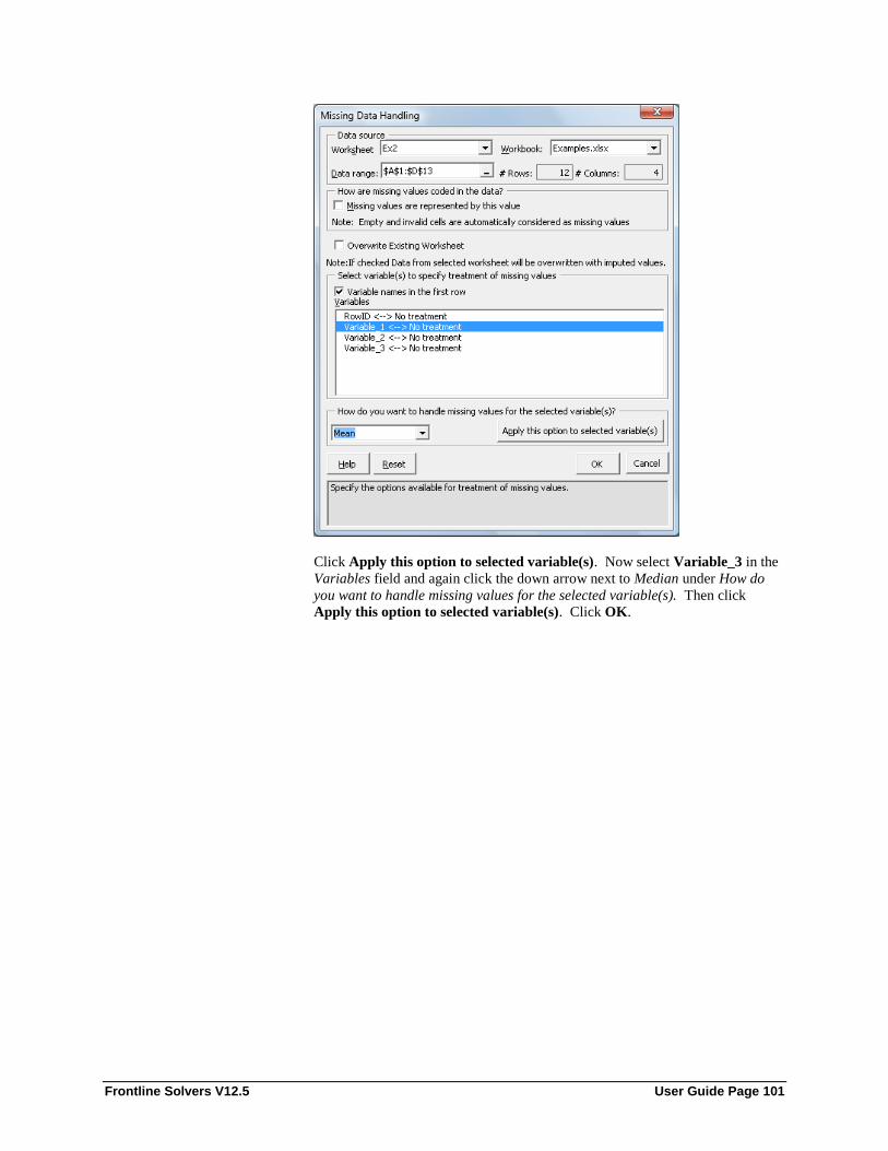
Frontline Solvers V12.5 User Guide Page 101
Click Apply this option to selected variable(s). Now select Variable_3 in the
Variables field and again click the down arrow next to Median under How do
you want to handle missing values for the selected variable(s). Then click
Apply this option to selected variable(s). Click OK.

Frontline Solvers V12.5 User Guide Page 102
The results are shown below.
As you can see, in the Variable_1 column, invalid or missing values have been
replaced with the mean calculated from the remaining values in the column.
(12.34, 34, 44, -433, 43, 34, 6743, 3, 4 & 3). The cells containing missing
values or invalid values in the Variable_3 column have been replaced by the
median of the remaining values in that column (12, 33, 44, 66, 33, 66, 22, 88, 55

Frontline Solvers V12.5 User Guide Page 103
& 79). The invalid data for Variable_2 remains since “No Treatment” was
selected for this variable.
Click the Ex3 worksheet tab. In this dataset, Variable_3 has been replaced with
date values.
Select cell A2 and click Transform -- Missing Data Handling on the
XLMiner ribbon to open the Missing Data Handling dialog. In this example, we
will replace the missing / invalid values for Variable_2 and Variable_3 with the
mode of each column.
On the Missing Data Handling dialog select Variable_2, click the down arrow
next to No Treatment under How do you want to handle values for the selected
variable(s), then select Mode. (The options Mean and Median do not appear in
the list since Variable_2 contains non-numeric values.) Click on Apply this
option to selected variable(s). Repeat these steps for Variable_3. Then click
OK.

Frontline Solvers V12.5 User Guide Page 104
The results are shown below.
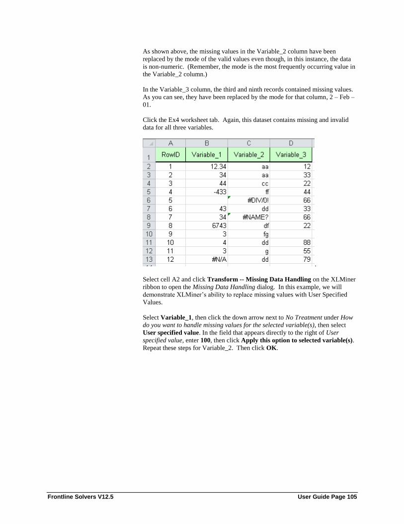
Frontline Solvers V12.5 User Guide Page 105
As shown above, the missing values in the Variable_2 column have been
replaced by the mode of the valid values even though, in this instance, the data
is non-numeric. (Remember, the mode is the most frequently occurring value in
the Variable_2 column.)
In the Variable_3 column, the third and ninth records contained missing values.
As you can see, they have been replaced by the mode for that column, 2 – Feb –
01.
Click the Ex4 worksheet tab. Again, this dataset contains missing and invalid
data for all three variables.
.
Select cell A2 and click Transform -- Missing Data Handling on the XLMiner
ribbon to open the Missing Data Handling dialog. In this example, we will
demonstrate XLMiner’s ability to replace missing values with User Specified
Values.
Select Variable_1, then click the down arrow next to No Treatment under How
do you want to handle missing values for the selected variable(s), then select
User specified value. In the field that appears directly to the right of User
specified value, enter 100, then click Apply this option to selected variable(s).
Repeat these steps for Variable_2. Then click OK.

Frontline Solvers V12.5 User Guide Page 106
The results are shown below.

Frontline Solvers V12.5 User Guide Page 107
As you can see, the missing values for Variable_1 and Variable_2 have replaced
by 100 while the values for Variable_3 remain untouched.
Click the Ex5 worksheet tab. In this dataset, the value -999 appears in all three
columns. This example will illustrate XLMiner’s ability to detect a given value
and replace that value with a user specified value.
Select cell A2 and click Transform -- Missing Data Handling on the XLMiner
ribbon to open the Missing Data Handling dialog.
Select Missing values are represented by this value and enter -999 in the field
that appears directly to the right of the option. Select Variable_1 in the
Variables field and instruct XLMiner to replace the contents of the cells
containing the value -999 with the mean of the remaining values in the column
Next, select Variable_2 in the Variables field and instruct XLMiner to replace
the contents of the cells containing -999 in this column with “zzz”. Finally,
select Variable_3 in the Variables field and instruct XLMiner to replace the
contents of the cells containing -999 in this column for the mode of the
remaining values in the column.

Frontline Solvers V12.5 User Guide Page 108
The results are shown below.
Note that in the Variable_1 column, the specified missing code (-999) is
replaced by the mean of the column. In the Variable_2 column, the missing

Frontline Solvers V12.5 User Guide Page 109
values have been replaced by the user specified value of “zzz” and for
variable_3 by the mode of the column.
Let’s take a look at one more dataset, Ex6, of Examples.xls.
Select cell A2 and click Transform -- Missing Data Handling to open the
Missing Data Handling dialog then apply the following procedures to the
indicated columns.
A. Select Missing values are represented by this value and enter 33 in
the field that appears directly to the right of the option.
B. Select Delete record for Variable_1’s treatment.
C. Select mode for Variable_2’s treatment
D. Specify the value 9999 for missing/invalid values for Variable_3.
E. Click OK.

Frontline Solvers V12.5 User Guide Page 110
See the output.

Frontline Solvers V12.5 User Guide Page 111
As shown above, records 7 and 12 have been deleted since Delete Record was
chosen for the treatment of missing values for Variable_1. In the Variable_2
column, the missing values have been replaced by the mode as indicated in the
Missing Data Handling dialog (shown above) except for record 7 which was
deleted. It is important to note that "Delete record" holds priority over any
other instruction in the Missing Data Handling feature.
In the Variable_3 column, we instructed XLMiner to treat 33 as a missing value.
As a result 33, and the additional missing values in this column (D4 and D10),
were replaced by the user specified value of 9999. Note: The value for
Variable_3 for record 12 was 33 which should have been replaced by 9999.
However, since Variable_1 contained a missing value for this record, the
instruction "Delete record" was executed first.
Options for Missing Data Handling The following options appear on the Missing Data Handling dialog.
Missing Values are represented by this value
If this option is selected, a value (either non-numeric or numeric) must be
provided in the field that appears directly to the right of the option. XLMiner
will treat this value as “missing” and will be handled per the instructions applied
in the Missing Data Handling dialog.
Note: XLMiner treats empty and invalid cells as missing values automatically.

Frontline Solvers V12.5 User Guide Page 112
Overwrite existing worksheet
If checked, XLMiner overwrites the data set with the new dataset in which all
the missing values are appropriately treated.
Variable names in the first Row
When this option is selected, XLMiner will list each variable according to the
first row in the selected data range. When the box is unchecked, XLMiner
follows the default naming convention, i.e., the variable in the first column of
the selected range will be called "Var1", the second column "Var2," etc.
Variables
Each variable and its selected treatment option are listed here.
How do you want to handle missing values for the selected variable(s)?
When a variable in the Variables field is selected, this option is enabled. Click
the down arrow to display the following options.
Delete record - If this option is selected, XLMiner will delete the entire record
if a missing or invalid value is found for that variable.
Mode - All missing values in the column for the variable specified will be
replaced by the mode - the value occurring most frequently in the remainder of
the column.
Mean - All missing values in the column for the variable specified will be
replaced by the mean - the average of the values in the remainder of the column.
Median - All missing values in the column for the variable specified will be
replaced by the median - the number that would appear in the middle of the
remaining column values if all values were written in ascending order.
User specified value – If selected, a value must be entered in the field that
appears directly to the right of this menu. XLMiner will replace all missing /
invalid values with this specified value.
No treatment - If this option is selected, no treatment will be applied to the
missing / invalid values for the selected variable.
Apply this option to selected variable(s)
Clicking this command button will apply the treatment option selected.
Reset
Resets treatment to No Treatment for all variables listed in the Variables field.
Also, deselects the Overwrite Existing Worksheet option if selected.
OK
Click to run the Missing Data Handling feature of XLMiner.

Frontline Solvers V12.5 User Guide Page 113
Binning Continuous Data
Introduction Binning a dataset is a process of grouping measured data into data classes. These
data classes can be used in various analyses. For example, in certain XLMiner
routines, continuous variables are not supported. The Binning utility can be
applied to these variables and then this new “binned-variable” can be chosen as
a categorical variable. In XLMiner, the user decides what values the binned
variable should take.
A variable can be binned in the following ways.
Equal count: When using this option, an equal number of bin intervals are
created based on the number of records present.
Rank: In this option each value in the variable is assigned a rank according to
the start and increment value. Users can specify the starting and increment
value.
Mean: The mean is calculated as the average of the values lying in the bin
interval. This mean value is assigned to each value of the variable that lies in
that interval.
Median: Records with the same binning value are counted and the median is
calculated on the input value. The median value is then assigned to the binned
variable.
Equal Interval: Equal interval is based on bin size. When this method is
selected, the whole range is divided into bins with bin sizes specified by the
user. The options of Rank and Mid value are available with this method.
Examples for Binning Continuous Data Open the Binning_Example.xlsx dataset by clicking Help – Examples on the
XLMiner ribbon.

Frontline Solvers V12.5 User Guide Page 114
Select a cell in the dataset, say A2, and click Transform -- Bin Continuous
Data on the XLMiner ribbon to open the Bin Continuous Data dialog shown
below.

Frontline Solvers V12.5 User Guide Page 115
Select x3 in the Variables field. The options are immediately activated. Under
Value in the binned variable is, enter 10 for Start and 3 for Interval, then click
Apply this option to the selected variable. The variable, x3, will appear in the
field labeled, Name of binned variable.

Frontline Solvers V12.5 User Guide Page 116
Now click OK. The results are shown below.

Frontline Solvers V12.5 User Guide Page 117
As specified, 5 bins were created starting with a rank of 10 and an interval of 3:
10, 13 (10 + 3), 16 (13 + 3), 19 (16 + 3), and 22 (19 + 3). The first five smallest
values (96, 104, 111, 113, 136) have been assigned to Bin 10. The next four
values in ascending order (148, 150, 151, 164) have been assigned to Bin 13.
The next five values in ascending order (168, 168, 173, 174, 175) have been
assigned to Bin 16. The next four values in ascending order (178, 192, 197,
199) have been assigned to Bin 19 and the last four values (202, 204, 245, 252)
have been assigned to Bin 22.
Though Bins to be with is set to Equal Count, the number of records in each
interval may not be essentially the same. Factors such as border values, total
number of records, etc. influence the number of records assigned to each bin.
XLMiner reports the binning intervals in the report as shown below.
The next example pins the value of the variable to the mean of the bin rather
than the rank of the bin.
Click back to Sheet1 and select cell A2, then click Transform – Bin
Continuous Data. Select Mean of the bin, rather than Rank of the bin for

Frontline Solvers V12.5 User Guide Page 118
Value in the binned variable. Leaving all remaining options at their defaults,
click Apply this option to the selected variable then click OK.

Frontline Solvers V12.5 User Guide Page 119
In the output, the Binned_x3 variable is equal to the mean of all the x3 variables
assigned to that bin. Let’s take the first record for an example. Recall, from the
previous example, the values from Bin 13: 148, 150, 151, 164. The mean of
these values is 153.25 ((148 + 150 + 151 + 164) / 4) which is the value for the
Binned_x3 variable for the first record.
Similarly, if we were to select the Median of the bin option, the Binned_x3
variable would equal the median of all x3 variables assigned to each bin.
The next example explores the Equal interval option.
Click back to Sheet1 and select any cell in the dataset, say, A2, then click
Transform – Bin Continuous Data on the XLMiner ribbon. Select x3 in the
Variables field, enter 4 for #bins for the variable, select Equal interval under
Bins to be made with, enter 12 for Start and 3 for Interval under Value in the
binned variable is, then click Apply this option to the selected variable.

Frontline Solvers V12.5 User Guide Page 120
Click OK – the output is shown below.
XLMiner calculates the interval as the Maximum value for the x3 variable -
Minimum value for the x3 variable) / #bins specified by the user or in this

Frontline Solvers V12.5 User Guide Page 121
instance (252 – 96) / 4 which equals 39. This means that the bins will be
assigned x3 variables in accordance to the following rules.
Bin 12: Values 96 – < 136
Bin 15: Values 136 – < 174
Bin 18: Values 174 – 213
Bin 21: Values 214 – 252
In the first record, x4 has a value of 151. As a result, this record has been
assigned to Bin 15 since 151 lies in the interval of Bin 15.
Click back to Sheet1 and select any cell in the dataset, say, A2, then click
Transform – Bin Continuous Data on the XLMiner ribbon. Select x3 in the
Variables field, enter 4 for #bins for the variable, select Equal interval under
Bins to be made with, select Mid Value for Value in the binned variable is, then
click Apply this option to the selected variable.
Then click OK. The output is shown below.

Frontline Solvers V12.5 User Guide Page 122
As shown in the output above, XLMiner created 4 bins with intervals from 90 to
130 (Bin 1), 130 – 170 (Bin 2), 170 – 210 (Bin 3), and 210 – 253 (Bin 4). The
value of the binned variable is the midpoint of each interval: 110 for Bin 1, 150
for Bin 2, 190 for Bin 3 and 210 for Bin 4. In the first record, x3’s value is 151.
Since this value lies in the interval for Bin 2 (130 – 170) the mid value of this
interval is reported for the Binned_x3 variable, 150. In the last record, x3’s
value is 174. Since this value lies in the interval for Bin 3 (170 – 210), the mid
value of this interval is reported for the Binned_x3 variable, 190.
Options for Binning Continuous Data The following options appear on the Bin Continuous Data dialog.

Frontline Solvers V12.5 User Guide Page 123
Variable names in the first row
If this option is selected, the list of variables in the Variables field will be listed
according to titles appearing in the first row of the dataset.
Name of the binned variable
Variable appearing here will be binned.
Show binning values in the output
Select this option to include the binning variables in the output report.
Name of binned variable
The name displayed here will appear for the binned variable in the output report.
#bins for the variable
Enter the number of desired bins here.

Frontline Solvers V12.5 User Guide Page 124
Equal count
When this option is selected, the binning procedure will assign an equal number
of records to each bin. Note: There is a possibility that the number of records in
a bin may not be equal due to factors such as border values, the number of
records being divisible by the number of bins, etc. The options for Value of the
binned variable for this process are Rank, Mean, and Median. See below for
explanations of each.
Equal interval
When this option is selected, the binning procedure will assign records to bins if
the record’s value falls in the interval of the bin. Bin intervals are calculated by
subtracting the Minimum variable value from the Maximum variable value and
dividing by the number of bins ((Max Value – Min Value) / # bins). The
options for Value of the binned variable for this process are Rank and Mid value.
See below for explanations of each.
Rank of the bin
When either the Equal count or the Equal interval option is selected, Rank of the
bin is enabled. When selected, the User has the option to specify the Start value
of the first bin and the Interval of each bin. Subsequent bin values will be
calculated as the previous bin + interval value.
Mean of the bin
When the Equal count option is selected, Mean of the bin is enabled. XLMiner
calculates the mean of all values in the bin and assigns that value to the binned
variable.
Median of the bin
When the Equal count option is selected, Median of the bin is enabled.
XLMiner finds the median of all values in the bin and assigns that value to the
binned variable.
Mid Value
When the Equal Interval option is selected, this option is enabled. The mid
value of the interval will be displayed on the output report for the assigned bin.
Apply this option to the selected variable
Click this command button to apply the selected options to the selected variable.

Frontline Solvers V12.5 User Guide Page 125
Transforming Categorical Data
Introduction Analysts often deal with data that is not numeric. Non numeric data values could
be text, alphanumeric (mix of text and numbers), or numeric values with no
numerical significance (such as a postal code). Such variables are called
'Categorical' variables, where every unique value of the variable is a separate
'category'.
Dealing with categorical data poses some limitations. For example, if your data
contained too many categories there would be a need to combine several
categories into one. In addition, perhaps you may desire to use a data mining
technique that requires numeric data rather than categorical data. The features
included in the Transform group address these requirements.
XLMiner provides options to transform data in the following ways:
1. By Creating Dummy Variables: When this feature is used, a string
variable is transformed into a dummy variable. XLMiner can handle string
variables with up to 30 distinct values. Imagine a variable called Language
which has data values English, French, German and Spanish. Running this
transformation will result in the creation of four new variables:
Language_English, Language_French, Language_German, and
Language_Spanish. Each of these variables will take on values of either 0
or 1 depending on the value of the Language variable in the record. For
instance, if a particular record has a German data value then among the
dummy variables created, Language_German will be 1 and others will be
zero.
In XLMiner, this procedure can be applied to all non-numeric categorical
variables in a dataset provided that each variable has less than 30 distinct
values.
2. Create Category Scores: In this feature, a string variable is converted into
a new numeric, categorical variable.
3. Reduce Categories: If you have more than 30 categories in a particular
variable, this utility helps you create a new categorical variable that reduces
the number of categories to 30. There are two different options to choose
from.
A. Option 1 assigns categories 1 through 29 to the 29 most frequently
occurring categories, and assigns category 30 to all remaining
categories
B. Option 2 maps multiple distinct category values in the original column
to a new category variable between 1 and 30.
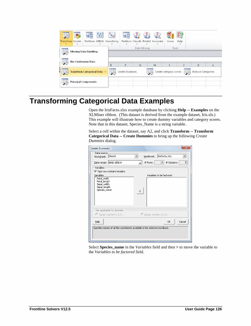
Frontline Solvers V12.5 User Guide Page 126
Transforming Categorical Data Examples Open the IrisFacto.xlsx example database by clicking Help -- Examples on the
XLMiner ribbon. (This dataset is derived from the example dataset, Iris.xls.)
This example will illustrate how to create dummy variables and category scores.
Note that in this dataset, Species_Name is a string variable.
Select a cell within the dataset, say A2, and click Transform -- Transform
Categorical Data -- Create Dummies to bring up the following Create
Dummies dialog.
Select Species_name in the Variables field and then > to move the variable to
the Variables to be factored field.

Frontline Solvers V12.5 User Guide Page 127
Click OK and view the output on the CategoryVar1 worksheet (inserted directly
after Sheet1.)
As shown in the output above, the variable, Species_name, is expressed as three
dummy variables: Species_name_Setosa, Species_name_Verginica and
Species_name_Versicolor. These new dummy variables are assigned values of
either 1, to indicate that the record belongs, or 0, to indicate that the record does
not belong. For example, Species_name_Setosa is assigned a value of 1 only
when the value of Species_name="Setosa" is in the dataset. Otherwise,
Species_name_Setosa = 0. The same is true for the two remaining dummy
variables i.e. Species_name_Verginica and Species_name_Versicolor.
In this example, XLMiner converted the string variable into three categorical
variables which resulted in a completely numeric dataset.
Click back to the dataset on Sheet1, select cell A2, and click Transform --
Transform Categorical Data -- Create Category Scores to open the XLMiner
Create category scores dialog shown below.

Frontline Solvers V12.5 User Guide Page 128
Select Species_name in the Variables field and click > to move the variable to
the Variables to be factored field. Keep the default option of Assign numbers
1,2,3....
Click OK and view the results on the CategoryVar2 worksheet which is inserted
directly to the right of Sheet 1 and the CategoryVar1 worksheets.

Frontline Solvers V12.5 User Guide Page 129
XLMiner has sorted the values of the Species_name variable alphabetically and
then assigned values of 1, 2 or 3 to each record depending on the species type.
(Starting from 1 because we selected Assign numbers 1,2,3.... To have XLMiner
start from 0, select the option Assign numbers 0, 1, 2,… on the Create Category
Scores dialog.) A variable, Species_name_ord is created to store these assigned
numbers. Again, XLMiner has converted this dataset to an entirely numeric
dataset.
Open the Iris.xls example dataset by clicking Help – Examples on the XLMiner
ribbon. Select a cell within the dataset, say cell A2, then click Transform --
Transform Categorical Data --> Reduce Categories to open the XLMiner
Reduce Categories dialog.
Select Petal_length as the variable, then select the Manually radio button under
Limit to 30 categories heading. In the Categories in selected variable box on
the right, all unique values of this variable are listed. Select all categories with
values less than 2; choose 1 for Category Number (Under Assign Category ID),
then click Apply. Repeat these steps for categories with values from 3 to 3.9
and apply a Category Number of 2. Continue repeating these steps until
category numbers from 4 thru 4.9 are assigned a Category Number of 3,
categories from 5 thru 5.9 are assigned a Category Number of 4, and categories
6 thru 6.9 are assigned a Category Number of 5.
Note: XLMiner is limited to 30 categories. If you pick By Frequency,
XLMiner assigns category numbers 1 through 29 to the most frequent 29 unique
values; and category number 30 to all other unique values. If you pick Manually,
XLMiner lets you map unique values to categories. You can pick multiple
unique values and map them to a single new category.

Frontline Solvers V12.5 User Guide Page 130
Click OK to produce the following output on the ReduceCat1 worksheet that is
inserted directly to the right of the Description worksheet.
In the output XLMiner has assigned new categories as shown in the column,
Petal_length CatNo, based on the choices made in the Reduce Categories
dialog.

Frontline Solvers V12.5 User Guide Page 131
Click back to the Data worksheet and click Transform – Transform
Categorical Data – Reduce Categories. Again select Petal_length in the
Variables field, but this time leave the default setting of By Frequency, then
click OK.

Frontline Solvers V12.5 User Guide Page 132
As you can see on the ReduceCat2 worksheet, XLMiner has classified the
Petal_length variable using 30 different categories. The values of 1.4 and 1.5
appear the most frequently (13 occurrences each) and have thus been labeled as
categories 1 and 2, respectively. The values of 4.5 and 5.1 each occur 8 times
and have thus been assigned to categories 3 and 4, respectively. The values of
1.3 and 1.6 occur seven times and, as a result, have been assigned to categories 5
and 6, respectively. Incremental category numbers are assigned to each
decreasing block of values until the 29th
category is assigned. All remaining
values are then lumped into the last category, 30.
Options for Transforming Categorical Data Explanations for options that appear on one of the three Transform Categorical
Data dialogs appear below.

Frontline Solvers V12.5 User Guide Page 133
Data Range
Either type the cell address directly into this field, or using the reference button;
select the required data range from the worksheet. If the cell pointer (active cell)
is already somewhere in the data range, XLMiner automatically picks up the
contiguous data range surrounding the active cell. When the data range is
selected XLMiner displays the number of records in the selected range.
First row contains headers
When this box is checked, XLMiner lists the variables according to the first row
of the selected data range. When the box is unchecked, XLMiner follows the
default naming convention, i.e., the variable in the first column of the selected
range will be called "Var1", the second column "Var2," etc.
Variables
This list box contains the names of the variables in the selected data range. To
select a variable, simply click to highlight, then click the > button. Use the
CTRL key to select multiple variables.
Options
The user can specify the number with which to start categorization 0 or 1. Select
the appropriate option.
Category Number
After manually selecting values from the list box, pick the category number to
assign. Click Apply to apply this mapping, or Reset to start over.

Frontline Solvers V12.5 User Guide Page 134
Principal Components Analysis
Introduction In the data mining field, databases with large amounts of variables are routinely
encountered. In most cases, the size of the database can be reduced by removing
highly correlated or superfluous variables. The accuracy and reliability of a
classification or prediction model produced from this resultant database will be
improved by the removal of these redundant and unnecessary variables. In
addition, superfluous variables increase the data-collection and data-processing
costs of deploying a model on a large database. As a result, one of the first steps
in data mining should be finding ways to reduce the number of independent or
input variables used in the model (otherwise known as dimensionality) without
sacrificing accuracy.
Principal component analysis (PCA) is a mathematical procedure that
transforms a number of (possibly) correlated variables into a smaller number of
uncorrelated variables called principal components. The objective of principal
component analysis is to reduce the dimensionality (number of variables) of the
dataset but retain as much of the original variability in the data as possible. The
first principal component accounts for the majority of the variability in the data,
the second principal component accounts for the majority of the remaining
variability, and so on.
A principal component analysis is concerned with explaining the variance
covariance structure of a high dimensional random vector through a few linear
combinations of the original component variables. Consider a database X with m
rows and n columns (X4x3)
X11 X12 X13
X21 X22 X23
X31 X32 X33
X41 X42 X43
1. The first step in reducing the number of columns (variables) in the X matrix
using the Principal Components Analysis algorithm is to find the mean of
each column.
(X11 + X21 + X31 + X41)/4 = Mu1
(X12 + X22 + X32 + X42)/4 = Mu2
(X13 + X23 + X33 + X43)/4 = Mu3
2. Next, the algorithm subtracts each element in the database by the mean
(Mu) thereby obtaining a new matrix, Ẍ, which also contains 4 rows and 3
columns.
X11 – Mu1 = Ẍ11 X12 – Mu2 = Ẍ12 X13 – Mu3 = Ẍ13
X21 – Mu1 = Ẍ21 X22 – Mu2 = Ẍ22 X23 – Mu3 = Ẍ23

Frontline Solvers V12.5 User Guide Page 135
X31 – Mu1 = Ẍ31 X32 – Mu2 = Ẍ32 X33 – Mu3 = Ẍ33
X41 – Mu1 = Ẍ41 X42 – Mu2 = Ẍ42 X43 – Mu3 = Ẍ43
3. Next, the PCA algorithm calculates the covariance or correlation matrix
(depending on the user’s preference) of the new Ẍ matrix.
4. Afterwards the algorithm calculates eigenvalues and eigenvectors from the
covariance matrix for each variable and lists these eigenvalues in order from
largest to smallest.
Larger eigenvalues denote that the variable should remain in the database.
Variables with smaller eigenvalues will be removed according to the user’s
preference.
5. XLMiner allows users to choose between selecting a fixed number of
components (variables) to be included in the “reduced” matrix (we will
refer to this new matrix as the Y matrix) or the smallest subset of variables
that “explains” or accounts for a certain percentage variance in the database.
Variables with eigenvalues below the chosen threshold will not be included
in the Y matrix. Assume that the user has chosen a fixed number of
variables (2) to be included in the Y matrix.
6. A new matrix V (containing eigenvectors based on the selected
eigenvalues) is formed.
7. The original matrix X which has 4 rows and 3 columns will be multiplied by
the V matrix, containing 4 rows and 2 columns. This matrix multiplication
results in the new reduced Y matrix, containing 4 rows and 2 columns.
In algebraic form, consider a p-dimensional random vector X = ( X1, X2, ..., Xp )
where p principal components of X are k univariate random variables Y1, Y2, ...,
Yk which are defined by the following formulae:
where the coefficient vectors l1, l2 ,..etc. are chosen such that they satisfy the
following conditions:
First Principal Component = Linear combination l1'X that maximizes Var(l1'X)
and || l1 || =1
Second Principal Component = Linear combination l2'X that maximizes
Var(l2'X) and || l2 || =1
and Cov(l1'X , l2'X) =0
jth Principal Component = Linear combination lj'X that maximizes Var(lj'X) and
|| lj || =1
and Cov(lk'X , lj'X) =0 for all k < j
These functions indicate that the principal components are those linear
combinations of the original variables which maximize the variance of the linear
combination and which have zero covariance (and hence zero correlation) with
the previous principal components.

Frontline Solvers V12.5 User Guide Page 136
It can be proved that there are exactly p such linear combinations. However,
typically, the first few principal components explain most of the variance in the
original data. As a result, instead of working with all the original variables X1,
X2, ..., Xp, you would typically first perform PCA and then use only the first two
or three principal components, say Y1 and Y2, in a subsequent analysis.
Examples for Principal Components Click Help – Examples on the XLMiner ribbon to open the example file
Utilities.xlsx. This example dataset gives data on 22 public utilities in the US.
Select a cell within the dataset, say A2, then click Transform – Principal
Components on the XLMiner ribbon to open the Principal Components dialog
shown below.

Frontline Solvers V12.5 User Guide Page 137
Select variables x1 to x8, then click the > command button to move them to the
Input variables field. (Perform error based clustering is not supported in the
PCA algorithm and is disabled). The figure below shows the first dialog box of
the Principal Components Analysis method. Click Next.

Frontline Solvers V12.5 User Guide Page 138
XLMiner provides two routines for specifying the number of principal
components: Fixed #components and Smallest # components explaining. The
Fixed # components method allows the user to specify a fixed number of
components, or variables, to be included in the “reduced” model . The Smallest
#components explaining method allows the user to specify a percentage of the
variance. When this method is selected XLMiner will calculate the minimum
number of principal components required to account for that percentage of the
variance.
In addition, XLMiner provides two methods for calculating the principal
components: using the covariance or the correlation matrix. When using the
correlation matrix method, the data will be normalized first before the method is
applied. (The dataset is normalized by dividing each variable by its standard
deviation.) Normalizing gives all variables equal importance in terms of
variability.1 If the covariance method is selected, the data will not be
normalized.
Select Use Correlation Matrix (Uses Standardized Variables). Then click
Next.
1 Shmueli, Galit, Nitin R. Patel, and Peter C. Bruce. Data Mining for Business Intelligence. 2nd ed. New Jersey: Wiley, 2010

Frontline Solvers V12.5 User Guide Page 139
On the Step 3 of 3 dialog, confirm Show principal components score is
selected, and then click Finish. This option displays an output matrix where the
columns are the principal components, the rows are the individual data records
and the value in each cell is the calculated score for that record on the relevant
principal component.
Two worksheets are inserted immediately after the Description worksheet:
PCA_Output1 and PCA_Scores1. The output from PCA_Output1 is shown
below.

Frontline Solvers V12.5 User Guide Page 140
The top section of the PCA_Output1 spreadsheet simply displays the number of
principal components created (as selected in the Step 2 of 3 dialog above), the
number of records in the dataset and the method chosen, Correlation matrix
(also selected in the Step 2 of 3 dialog).
The bottom portion of the PCA_Output worksheet displays the principal
component table. The maximum value for Component 1 corresponds to x2
(.5712). This signifies that the first principal component is measuring the effect
of x2 on the utility companies. Likewise, the second component appears to be
measuring the effect of x4 on the utility companies (.4091). The first
component accounts for 27.16% of the variance while the second component
accounts for 23.75%. Together, these two components account for more than
50% of the total variation.
The output from the PCA_Scores1 worksheet is below. This table holds the
weighted averages of the normalized variables (after each variable’s mean is
subtracted). (This matrix is described in the 2nd
step of the PCA algorithm - see
Introduction above.)

Frontline Solvers V12.5 User Guide Page 141
Click back to the Data worksheet, select any cell in the dataset, and then click
Transform – Principal Components. Cells x1 through x8 are already selected
so simply click Next on this dialog to advance to the Step 2 of 3 dialog.
This time, select Smallest # of components explaining, enter 50 for % of
variance, select Use Correlation Matrix, and then click Finish.

Frontline Solvers V12.5 User Guide Page 142
As you can see from the output worksheet PCA_Output2, only the first two
components are included in the output file since these two components account
for over 50% of the variation.
After applying the Principal Components Analysis algorithm, users may proceed
to analyze their dataset by applying additional data mining algorithms featured
in XLMiner.
Options for Principal Components Analysis Options for Principal Components Analysis appear on the Step 2 of 3 and Step 3
of 3 dialogs. For more information on the Step1 of 3 dialog, please see the
Common Dialog Options section in the Introduction to XLMiner chapter.
Principal Components
Select the number of principal components displayed in the output.

Frontline Solvers V12.5 User Guide Page 143
Fixed # of components
Specify a fixed number of components by selecting this option and entering an
integer value from 1 to n where n is the number of Input variables selected in
the Step 1 of 3 dialog.
Smallest #components explaining
Select this option to specify a percentage. XLMiner will calculate the minimum
number of principal components required to account for that percentage of
variance.
Method
To compute Principal Components the data is matrix multiplied by a
transformation matrix. This option lets you specify the choice of calculating this
transformation matrix.
Use Covariance matrix
The covariance matrix is a square, symmetric matrix of size n x n (number of
variables by number of variables). The diagonal elements are variances and the
off-diagonals are covariances. The eigenvalues and eigenvectors of the
covariance matrix are computed and the transformation matrix is defined as the
transpose of this eigenvector matrix. If the covariance method is selected, the
dataset should first be normalized. One way to organize the data is to divide
each variable by its standard deviation. Normalizing gives all variables equal
importance in terms of variability.2
Use Correlation matrix
An alternative method is to derive the transformation matrix on the eigenvectors
of the correlation matrix instead of the covariance matrix. The correlation
matrix is equivalent to a covariance matrix for the data where each variable has
been standardized to zero mean and unit variance. This method tends to
equalize the influence of each variable, inflating the influence of variables with
relatively small variance and reducing the influence of variables with high
variance.
2 Shmueli, Galit, Nitin R. Patel, and Peter C. Bruce. Data Mining for Business Intelligence. 2nd ed. New Jersey: Wiley, 2010

Frontline Solvers V12.5 User Guide Page 144
Show principal components score
This option results in the display of a matrix in which the columns are the
principal components, the rows are the individual data records, and the value in
each cell is the calculated score for that record on the relevant principal
component.

Frontline Solvers V12.5 User Guide Page 145
k-Means Clustering
Introduction Cluster Analysis, also called data segmentation, has a variety of goals which all
relate to grouping or segmenting a collection of objects (also called
observations, individuals, cases, or data rows) into subsets or "clusters". These
“clusters” are grouped in such a way that the observations included in each
cluster are more closely related to one another than objects assigned to different
clusters. The most important goal of cluster analysis is the notion of the degree
of similarity (or dissimilarity) between the individual objects being clustered.
There are two major methods of clustering -- hierarchical clustering and k-
means clustering. (See the k-means clustering chapter for information on this
type of clustering analysis.)
This chapter explains the k-Means Clustering algorithm. The goal of this
process is to divide the data into a set number of clusters (k) and to assign each
record to a cluster while minimizing the distribution within each cluster. A non-
hierarchical approach to forming good clusters is to specify a desired number of
clusters, say, k, then assign each case (object) to one of k clusters so as to
minimize a measure of dispersion within the clusters. A very common measure
is the sum of distances or sum of squared Euclidean distances from the mean of
each cluster. The problem can be set up as an integer programming problem but
because solving integer programs with a large number of variables is time
consuming, clusters are often computed using a fast, heuristic method that
generally produces good (but not necessarily optimal) solutions. The k-means
algorithm is one such method.
Examples for k-Means Clustering Click Help – Examples on the XLMiner ribbon and open the example file
Wine.xlsx. As shown in the figure below, each row in this example dataset
represents a sample of wine taken from one of three wineries (A, B or C). In this
example, the Type variable representing the winery is ignored and the clustering
is performed simply on the basis of the properties of the wine samples (the
remaining variables).

Frontline Solvers V12.5 User Guide Page 146
Select a cell within the dataset, say A2, and then click XLMiner – Cluster – k-
Means Clustering. The following dialog box will appear.
Select all variables under Variables in data source except Type, then click the >
button to shift the selected variables to the Input variables field.

Frontline Solvers V12.5 User Guide Page 147
Afterwards, click Next to advance to the Step 2 of 3 dialog.
Enter 8 for # Clusters to be formed. This is the parameter k in the k-means
clustering algorithm. The number of clusters should be at least 2 and at most the
number of observations in the data range. It is a good idea to set k to several
different values and evaluate the output from each.
Enter 10 for # Iterations. The value for this option determines how many times
the program will start with an initial partition and complete the clustering
algorithm. The configuration of clusters (and how good a job they do of
separating the data) may differ from one starting partition to another. The
program will go through the specified number of iterations, and select the cluster
configuration that minimizes the distance measure.
Select the Random Starts option. When this option is selected, the algorithm
will start building the model from any random point. Enter 5 for No. of starts.
XLMiner will generate five cluster sets and will generate the output based on the
best cluster. Enter 12345 for Fixed Seed. A value specified here will ensure the
same starting points each time the algorithm is run.
If Fixed start were to be selected, XLMiner would build the model with a single
fixed starting point.

Frontline Solvers V12.5 User Guide Page 148
Click Next.
On the Step 3 of 3 dialog, select Show data summary (default) and Show
distances from each cluster center (default). Then click Finish.
The K-Means Clustering method will start with k initial clusters as specified by
the user. At each iteration, the records are assigned to the cluster with the closest
centroid, or center. After each iteration, the distance from each record to the
center of the cluster is calculated. These two steps are repeated (the record
assignment and distance calculation) until the redistribution of a record results in
an increased distance value.
When the user specifies a random start, the algorithm generates the k cluster
centers randomly and fits the data points in those clusters. This process is
repeated for as many random starts as the user specifies. The output will be
based on the clusters that exhibit the best fit.
The worksheet, KM_Output1 is inserted immediately after the Description
worksheet. In the top section of the output worksheet, the options that were
selected are listed.

Frontline Solvers V12.5 User Guide Page 149
In the middle section of the output worksheet, XLMiner has calculated the sum
of the squared distances and has determined the start with the lowest Sum of
Square Distance as the Best Start (#3). After the Best Start is determined,
XLMiner generates the remaining output using the Best Start as the starting
point.
In the bottom portion of the output worksheet, XLMiner has listed the "cluster
centers" (shown below). The upper box shows the variable values at the cluster
centers. As you can see, the first cluster has the highest average
Nonflavanoid_Phenol and Ash_Alcalinity, and a very high Magnesium average.
Compare this cluster to Cluster 5 which has the highest average Proline,
Flavanoids, and Color_Intensity, and a very high Malic_Acid average.
The lower box shows the distance between the cluster centers. From the values
in this table, we can discern that cluster 5 is very different from cluster 6 due to
the high distance value of 1,484.51 and cluster 7 is very close to cluster 3 (low
distance value of 31.27). It is possible that these two clusters could be merged
into one cluster.

Frontline Solvers V12.5 User Guide Page 150
The Data Summary displays the number of records (observations) included in
each cluster and the average distance from cluster members to the center of each
cluster. As you can see, cluster 2 has the highest average distance and includes
78 records. Compare this cluster to cluster 6 which has 0 members.
Click the KM_Clusters1 worksheet. This worksheet displays the cluster to
which each record is assigned and the distance to each of the clusters. Note that,
for record 5, the distance to cluster 1 is the minimum distance, so record 5 is
assigned to cluster 1.
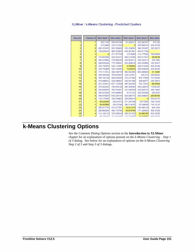
Frontline Solvers V12.5 User Guide Page 151
k-Means Clustering Options See the Common Dialog Options section in the Introduction to XLMiner
chapter for an explanation of options present on the k-Means Clustering – Step 1
of 3 dialog. See below for an explanation of options on the k-Means Clustering
Step 2 of 3 and Step 3 of 3 dialogs.

Frontline Solvers V12.5 User Guide Page 152
Clustering Method
At this time, XLMiner supports standard clustering only.

Frontline Solvers V12.5 User Guide Page 153
Normalize input data
If this option is selected, XLMiner will normalize the input data before applying
the k-Means Clustering algorithm. Normalizing the data is important to ensure
that the distance measure accords equal weight to each variable. Without
normalization, the variable with the largest scale will dominate the measure.
# Clusters
Enter the number of final clusters (k) to be formed here. The number of clusters
should be at least 2 and at most the number of observations in the data range.
This value should be based on your knowledge of the data and the number of
projected clusters. It is a good idea to repeat the procedure with several
different k values.
# Iterations
Enter the number of times the program will perform the clustering algorithm.
The configuration of clusters (and how good a job they do of separating the
data) may differ from one starting partition to another. The algorithm will
complete the specified number of iterations and select the cluster configuration
that minimizes the distance measure.
Options
If Fixed start is selected, XLMiner will start building the model with a single
fixed starting point. If Random starts is selected, the algorithm will start at any
random point.
If Random starts is selected, two additional options are enabled: No. of Starts
and Seed. Enter the number of desired clusters for No. of Starts. XLMiner will
complete the desired number of clusters and generate the output for the best
cluster set. To enter a fixed seed, select Fixed and then enter an integer value.
Show data summary
Select this option to display the data summary in the k-Means Clustering output.
Show distances from each cluster center
Select this option to display the distances from each cluster center in the k-
Means Clustering output.

Frontline Solvers V12.5 User Guide Page 154
Hierarchical Clustering
Introduction
Cluster Analysis, also called data segmentation, has a variety of goals. All relate
to grouping or segmenting a collection of objects (also called observations,
individuals, cases, or data rows) into subsets or "clusters", such that those within
each cluster are more closely related to one another than objects assigned to
different clusters. The most important goal of cluster analysis is the notion of
degree of similarity (or dissimilarity) between the individual objects being
clustered. There are two major methods of clustering -- hierarchical clustering
and k-means clustering. (See the k-means clustering chapter for information on
this type of clustering analysis.)
In hierarchical clustering the data are not partitioned into a particular cluster in a
single step. Instead, a series of partitions takes place, which may run from a
single cluster containing all objects to n clusters each containing a single object.
Hierarchical Clustering is subdivided into agglomerative methods, which
proceed by a series of fusions of the n objects into groups, and divisive methods,
which separate n objects successively into finer groupings. The hierarchical
clustering technique employed by XLMiner is an Agglomerative technique.
Hierarchical clustering may be represented by a two dimensional diagram
known as a dendrogram which illustrates the fusions or divisions made at each
successive stage of analysis. An example of such a dendrogram is given below:
Agglomerative methods
An agglomerative hierarchical clustering procedure produces a series of
partitions of the data, Pn, Pn-1, ....... , P1. The first Pn consists of n single object
'clusters', the last P1, consists of a single group containing all n cases.
At each particular stage the method joins the two clusters which are closest
together (most similar). (At the first stage, this amounts to joining together the
two objects that are closest together, since at the initial stage each cluster has
one object.)

Frontline Solvers V12.5 User Guide Page 155
Differences between methods arise because of the different methods of defining
distance (or similarity) between clusters. Several agglomerative techniques will
now be described in detail.
Single linkage clustering
One of the simplest agglomerative hierarchical clustering method is single
linkage, also known as the nearest neighbor technique. The defining feature of
this method is that distance between groups is defined as the distance between
the closest pair of objects, where only pairs consisting of one object from each
group are considered.
In the single linkage method, D(r,s) is computed as
D(r,s) = Min { d(i,j) : Where object i is in cluster r and object j is cluster s }
Here the distance between every possible object pair (i,j) is computed, where
object i is in cluster r and object j is in cluster s. The minimum value of these
distances is said to be the distance between clusters r and s. In other words, the
distance between two clusters is given by the value of the shortest link between
the clusters.
At each stage of hierarchical clustering, the clusters r and s, for which D(r,s) is
minimum, are merged.
This measure of inter-group distance is illustrated in the figure below:
Complete linkage clustering
The complete linkage, also called farthest neighbor, clustering method is the
opposite of single linkage. In this clustering method, the distance between
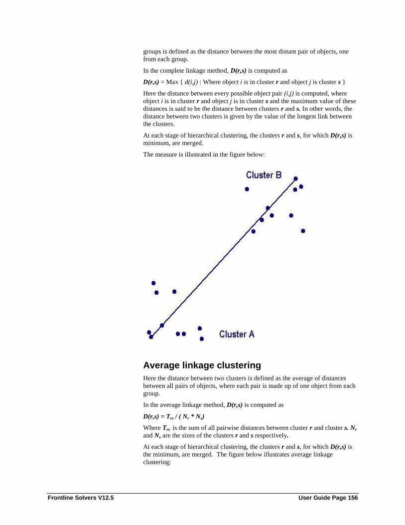
Frontline Solvers V12.5 User Guide Page 156
groups is defined as the distance between the most distant pair of objects, one
from each group.
In the complete linkage method, D(r,s) is computed as
D(r,s) = Max { d(i,j) : Where object i is in cluster r and object j is cluster s }
Here the distance between every possible object pair (i,j) is computed, where
object i is in cluster r and object j is in cluster s and the maximum value of these
distances is said to be the distance between clusters r and s. In other words, the
distance between two clusters is given by the value of the longest link between
the clusters.
At each stage of hierarchical clustering, the clusters r and s, for which D(r,s) is
minimum, are merged.
The measure is illustrated in the figure below:
Average linkage clustering
Here the distance between two clusters is defined as the average of distances
between all pairs of objects, where each pair is made up of one object from each
group.
In the average linkage method, D(r,s) is computed as
D(r,s) = Trs / ( Nr * Ns)
Where Trs is the sum of all pairwise distances between cluster r and cluster s. Nr
and Ns are the sizes of the clusters r and s respectively.
At each stage of hierarchical clustering, the clusters r and s, for which D(r,s) is
the minimum, are merged. The figure below illustrates average linkage
clustering:

Frontline Solvers V12.5 User Guide Page 157
Average group linkage
With this method, groups once formed are represented by their mean values for
each variable, that is, their mean vector, and inter-group distance is now defined
in terms of distance between two such mean vectors.
In the average group linkage method, the two clusters r and s are merged such
that, after merging, the average pairwise distance within the newly formed
cluster, is minimized. Suppose we label the new cluster formed by merging
clusters r and s, as t. Then D(r,s) , the distance between clusters r and s is
computed as
D(r,s) = Average { d(i,j) : Where observations i and j are in cluster t, the cluster
formed by merging clusters r and s }
At each stage of hierarchical clustering, the clusters r and s, for which D(r,s) is
minimized, are merged. In this case, those two clusters are merged such that the
newly formed cluster, on average, will have minimum pairwise distances
between the points.
Ward's hierarchical clustering method
Ward (1963) proposed a clustering procedure seeking to form the partitions Pn, P
n-1,........, P1 in a manner that minimizes the loss associated with each grouping, and
to quantify that loss in a form that is readily interpretable. At each step in the
analysis, the union of every possible cluster pair is considered and the two
clusters whose fusion results in minimum increase in 'information loss' are
combined. Information loss is defined by Ward in terms of an error sum-of-
squares criterion, ESS.
The rationale behind Ward's proposal can be illustrated most simply by
considering univariate data. Suppose for example, 10 objects have scores (2, 6,
5, 6, 2, 2, 2, 2, 0, 0, 0) on some particular variable. The loss of information that

Frontline Solvers V12.5 User Guide Page 158
would result from treating the ten scores as one group with a mean of 2.5 is
represented by ESS given by,
ESS One group = (2 -2.5)2 + (6 -2.5)
2 + ....... + (0 -2.5)
2 = 50.5
On the other hand, if the 10 objects are classified according to their scores into
four sets,
{0,0,0}, {2,2,2,2}, {5}, {6,6}
The ESS can be evaluated as the sum of squares of four separate error sums of
squares
ESS One group = ESS group1 + ESSgroup2 + ESSgroup3 + ESSgroup4 = 0.0
Clustering the 10 scores into 4 clusters results in no loss of information.
Examples of Hierarchical Clustering The utilities.xlsx example dataset (shown below) holds corporate data on 22 US
public utilities. This example will illustrate how a user would use XLMiner to
perform a cluster analysis using hierarchical clustering.
An example where clustering would be useful is a study to predict the cost
impact of deregulation. To perform the requisite analysis, economists would be
required to build a detailed cost model of the various utilities. It would save a
considerable amount of time and effort if we could cluster similar types of
utilities, build a detailed cost model for just one ”typical” utility in each cluster,
then scale up from these models to estimate results for all utilities.
Each record includes 8 observations. Before we can use a clustering technique,
the data must be “normalized” or “standardized”. A popular method for
normalizing continuous variables is to divide each variable by its standard
deviation. After the variables are standardized, the distance can be computed
between clusters using the Euclidean metric.
Open the Utilities.xlsx example dataset by clicking Help – Examples on the
XLMiner ribbon.
An explanation of the variables is below.

Frontline Solvers V12.5 User Guide Page 159
Select any cell in the dataset, for example A2, then click Cluster --
Hierarchical Clustering to bring up the Hierarchical Clustering dialog.
Select variables x1 through x8 in the Variables field, then click > to move the
selected variables to the Selected variables field.

Frontline Solvers V12.5 User Guide Page 160
Then click Next to advance to the Step 2 of 3 dialog.
At the top of the dialog, select Normalize input data. When this option is
selected, XLMiner will normalize the data by subtracting the variable’s mean
from each observation and dividing by the standard deviation. Normalizing the
data is important to ensure that the distance measure accords equal weight to
each variable -- without normalization, the variable with the largest scale will
dominate the measure.

Frontline Solvers V12.5 User Guide Page 161
Under Similarity measure, Euclidean distance is selected by default. The
Hierarchical clustering method uses the Euclidean Distance as the similarity
measure for raw numeric data. When the data is binary the remaining two
options, Jaccard's coefficients and Matching coefficients are enabled.
Under Clustering method, select Average group linkage. Recall from the
Introduction to this chapter, the average group linkage method calculates the
average distance of all possible distances between each record in each cluster.
Click Next.
On the Step 3 of 3 dialog, select Draw dendrogram and Show cluster
membership. Enter 4 for the # Clusters. Then click Finish. XLMiner will
create four clusters using the Average group linkage method. The output
worksheet HC_Output1 is inserted immediately after the Description worksheet.
This output details the history of the cluster formation. Initially, each individual
case is considered its own cluster (single member in each cluster). Since there
are 21 records, XLMiner begins the method with # clusters = # cases. At stage

Frontline Solvers V12.5 User Guide Page 162
1, above, clusters (i.e. cases) 10 and 13 were found to be closer together than
any other two clusters (i.e. cases), so they are joined together in a cluster called
Cluster 10. At this point there is one cluster with two cases (cases 10 and 13),
and 19 additional clusters that still have just one case in each. At stage 2,
clusters 7 and 12 are found to be closer together than any other two clusters, so
they are joined together into cluster 7.
This process continues until there is just one cluster. At various stages of the
clustering process, there are different numbers of clusters. A graph called a
dendrogram illustrates these steps.
In the above dendrogram, the Sub Cluster IDs are listed along the x-axis (in an
order convenient for showing the cluster structure). The y-axis measures inter-
cluster distance. Consider cases 10 and 13 -- they have an inter-cluster distance
of 1.51. No other cases have a smaller inter-cluster distance, so 10 and 13 are
joined into one cluster, indicated by the horizontal line linking them. Next, we
see that cases 7 and 12 have the next smallest inter-cluster distance, so they are
joined into one cluster. The next smallest inter-cluster distance is between
clusters 14 and 19 and so on.
If we draw a horizontal line through the diagram at any level on the y-axis (the
distance measure), the vertical cluster lines that intersect the horizontal line
indicate clusters whose members are at least that close to each other. If we draw
a horizontal line at distance = 2.3, for example, we see that there are 11 clusters.
In addition, we can see that a case can belong to multiple clusters, depending on
where we draw the line (i.e. how close we require the cluster members to be to
each other).
For purposes of assigning cases to clusters, we must specify the number of
clusters in advance. In this example, we specified a limit of 4.
If the number of training rows exceeds 30 then the dendrogram also displays
Cluster Legends.
The HC_Clusters1 output worksheet includes the following table.

Frontline Solvers V12.5 User Guide Page 163
This table displays the assignment of each record to the four clusters.
This next example illustrates k-Means Clustering when the data represents the
distance between the ith
and jth
records. (When applied to raw data, Hierarchical
clustering converts the data into the distance matrix format before proceeding
with the clustering algorithm. Providing the distance measures in the data
requires one less step for the Hierarchical clustering algorithm.)
Select a cell in the database, say A2, click XLMiner – Help – Examples and
open the file, DistMatrix.xls. Then, click XLMiner – Cluster – Hierarchical
Clustering to open the following dialog.
Click the down arrow next to Data Type and select Distance Matrix.
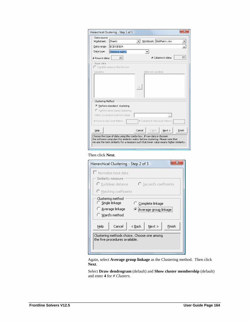
Frontline Solvers V12.5 User Guide Page 164
Then click Next.
Again, select Average group linkage as the Clustering method. Then click
Next.
Select Draw dendrogram (default) and Show cluster membership (default)
and enter 4 for # Clusters.

Frontline Solvers V12.5 User Guide Page 165
Then click Finish.
Output worksheets, HC_Output1, HC_Clusters1, and HC_Dendrogram1 are
inserted immediately after Sheet1.
The Clustering Stages output (included on the HC_Output1 worksheet) is shown
below.
The Dendrogram output (included on the HC_Dendrogram1 worksheet) is
shown below.
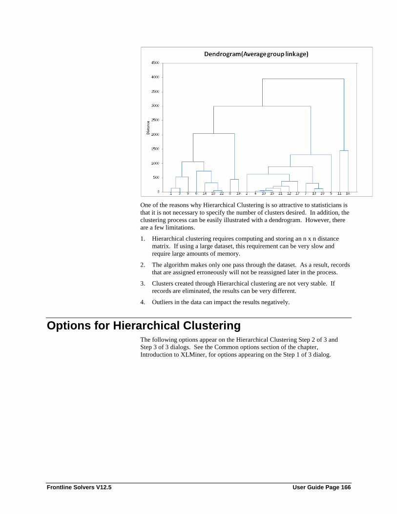
Frontline Solvers V12.5 User Guide Page 166
One of the reasons why Hierarchical Clustering is so attractive to statisticians is
that it is not necessary to specify the number of clusters desired. In addition, the
clustering process can be easily illustrated with a dendrogram. However, there
are a few limitations.
1. Hierarchical clustering requires computing and storing an n x n distance
matrix. If using a large dataset, this requirement can be very slow and
require large amounts of memory.
2. The algorithm makes only one pass through the dataset. As a result, records
that are assigned erroneously will not be reassigned later in the process.
3. Clusters created through Hierarchical clustering are not very stable. If
records are eliminated, the results can be very different.
4. Outliers in the data can impact the results negatively.
Options for Hierarchical Clustering The following options appear on the Hierarchical Clustering Step 2 of 3 and
Step 3 of 3 dialogs. See the Common options section of the chapter,
Introduction to XLMiner, for options appearing on the Step 1 of 3 dialog.

Frontline Solvers V12.5 User Guide Page 167
Data Type
The Hierarchical clustering method can be used on raw data as well as the data
in Distance Matrix format. Choose the appropriate option to fit your dataset.

Frontline Solvers V12.5 User Guide Page 168
Normalize input data
Normalizing the data is important to ensure that the distance measure accords
equal weight to each variable -- without normalization, the variable with the
largest scale will dominate the measure.
Similarity Measures
The Hierarchical clustering uses the Euclidean Distance as the similarity
measure for working on raw numeric data. When the data is binary, the
remaining two options, Jaccard's coefficients and Matching coefficient are
enabled.
Suppose we have binary values for all the xij ’s. See the table below for
individual i’s and j’s.
The most useful similarity measures in this situation are:
Jaccard’s coefficient = d/(b+c+d). This coefficient ignores zero matches.
The matching coefficient = (a + d)/p.
Clustering Method
See the introduction to this chapter for descriptions of each method.
Draw Dendrogram
Select this option to have XLMiner create a dendrogram to illustrate the
clustering process.
Show cluster membership
Select this option to display the cluster number (ID) to which each record is
assigned by the routine.

Frontline Solvers V12.5 User Guide Page 169
# Clusters
Recall that the agglomerative method of hierarchical clustering continues to
form clusters until only one cluster is left. This option lets you stop the process
at a given number of clusters.

Frontline Solvers V12.5 User Guide Page 170
Exploring a Time Series Dataset
Introduction Time series datasets contain a set of observations generated sequentially in time.
Organizations of all types and sizes utilize time series datasets for analysis and
forecasting for predicting next year’s sales figures, raw material demand,
monthly airline bookings, etc. .
Example of a time series dataset: Monthly airline bookings.
A time series model is first used to obtain an understanding of the underlying
forces and structure that produced the data and then secondly, to fit a model that
will predict future behavior. In the first step, the analysis of the data, a model is
created to uncover seasonal patterns or trends in the data, for example bathing
suit sales in June. In the second step, forecasting, the model is used to predict
the value of the data in the future, for example, next year’s bathing suit sales.
Separate modeling methods are required to create each type of model.
XLMiner features two techniques for exploring trends in a dataset, ACF
(Autocorrelation function) and PACF (Partial autocorrelation function). These
techniques help the user to explore various patterns in the data which can be
used in the creation of the model. After the data is analyzed, a model can be fit
to the data using XLMiner’s ARIMA method.
Autocorrelation (ACF)
Autocorrelation (ACF) is the correlation between neighboring observations in a
time series. When determining if an autocorrelation exists, the original time
series is compared to the “lagged” series. This lagged series is simply the
original series moved one time period forward (xn vs xn+1). Suppose there are 5
time based observations: 10, 20, 30, 40, and 50. When lag = 1, the original
series is moved forward one time period. When lag = 2, the original series is
moved forward two time periods.

Frontline Solvers V12.5 User Guide Page 171
Day Observed Value Lag-1 Lag-2
1 10
2 20 10
3 30 20 10
4 40 30 20
5 50 40 30
The autocorrelation is computed between the original series and the lag-1 series
using the Excel CORREL function. In a similar manner, the lag-2
autocorrelation is computed between the original series and the lag-2 series.
XLMiner’s ACF utility directly computes the autocorrelations of the series at
different lags.
The two red horizontal lines on the graph above delineate the Upper confidence
level (UCL) and the Lower confidence level (LCL). If the data is random, then
the plot should be within the UCL and LCL. If the plot exceeds either of these
two levels, as seen in the plot above, then it can be presumed that some
correlation exists in the data.
Partial Autocorrelation Function (PACF)
This technique is used to compute and plot the partial autocorrelations between
the original series and the lags. However, PACF eliminates all linear
dependence in the time series beyond the specified lag.
ARIMA An ARIMA (autoregressive integrated moving-average models) model is a
regression-type model that includes autocorrelation. The basic assumption in
estimating the ARIMA coefficients is that the data are stationary, that is, the
trend or seasonality cannot affect the variance. This is generally not true. To
achieve the stationary data, XLMiner will first apply “differencing”: ordinary,
seasonal or both.
After XLMiner fits the model, various results will be available. The quality of
the model can be evaluated by comparing the time plot of the actual values with
the forecasted values. If both curves are close, then it can be assumed that the
model is a good fit. The model should expose any trends and seasonality, if any
exist. If the residuals are random then the model can be assumed a good fit.
However, if the residuals exhibit a trend, then the model should be refined.
Fitting an ARIMA model with parameters (0,1,1) will give the same results as

Frontline Solvers V12.5 User Guide Page 172
exponential smoothing. Fitting an ARIMA model with parameters (0,2,2) will
give the same results as double exponential smoothing.
Partitioning
To avoid over fitting of the data and to be able to evaluate the predictive
performance of the model on new data, we must first partition the data into
training and validation sets, and possibly a test set, using XLMiner’s time series
partitioning utility. After the data is partitioned, ACF, PACF, and ARIMA can
be applied to the dataset.
Examples for Time Series Analysis The examples below illustrate how XLMiner can be used to explore the data to
uncover trends and seasonalities. Click Help – Examples on the XLMiner
ribbon and open the example dataset, Income.xlsx. This dataset contains the
average income of tax payers by state.
Typically the following steps are performed in a time series analysis.
1. The data is first partitioned into two sets with 60% of the data assigned to
the training set and 40% of the data assigned to validation.
2. Exploratory techniques are applied to both the training and validation sets.
If the results are in synch then the model can be fit. If the ACF and PACF
plots are the same, then the same model can be used for both sets.
3. The model is fit using the ARIMA method.
4. When we fit a model using the ARIMA method, XLMiner displays the ACF
and PACF plots for residuals. If these plots are in the band of UCL and
LCL then it indicates that the residuals are random and the model is
adequate.
5. If the residuals are not within the bands, then some correlation exists, and
the model should be improved.
First we must perform a partition on the data. Select a cell within the dataset,
such as A2, then click Partition within the Time Series group on the XLMiner
ribbon to open the following dialog.

Frontline Solvers V12.5 User Guide Page 173
Select Year under Variables and click > to define the variable as the Time
Variable. Select the remaining variables under Variables and click > to include
them in the partitioned data.
Select Specify #Records under Specify Partitioning Options. Then select
Specify Percentages under Specify Percentages for Partitioning. Enter 50 for
the number of Training Set records and 21 for the number of Validation Set
records.

Frontline Solvers V12.5 User Guide Page 174
Click OK. The Data_PartitionTS1 worksheet will be inserted directly behind
the Description worksheet.
Note in the output above, the partitioning method is sequential (rather than
random). The first 50 observations have been assigned to the training set and
the remaining 21 observations have been assigned to the validation set.
Select a cell on the Data_PartitionTS1 worksheet then click ARIMA –
Autocorrelations on the XLMiner ribbon to display the ACF dialog.

Frontline Solvers V12.5 User Guide Page 175
Select CA as the Selected variable, enter 10 for both ACF Parameters for
Training Data and ACF Parameters for Validation Data. Then select Plot ACF
chart.
Click OK. The worksheet ACF_Output1 will be inserted directly after the
Data_PartitionTS1 worksheet.
Both ACF functions show a definite pattern where the autocorrelation decreases
as the number of lags increases. Since the pattern does not repeat, it can be
assumed that no seasonality is included in the data. In addition, since both
charts exhibit a similar pattern, we can fit the same model to both the validation
and training sets.
Click back to the Data_PartitionTS1 worksheet and click ARIMA -- Partial
Autocorrelations to open the PACF dialog as shown below.

Frontline Solvers V12.5 User Guide Page 176
Select CA under Variables in input data, then click > to move the variable to
Selected variable. Enter 40 for Maximum Lag for PACF Parameters for
Training Data and 15 PACF Parameters for Validation Data. Select Plot
PACF chart.
Click OK. The worksheet, PACF_Output1, is inserted directly after the
ACF_Output1 worksheet. Both PACF plots show similar patterns in both the

Frontline Solvers V12.5 User Guide Page 177
validation and training sets. As a result, we can use the same model for both
sets.
PACF Output for Training Data
PACF Output for Validation Data
The PACF function shows a definite pattern which means there is a trend in the
data. However, since the pattern does not repeat, we can conclude that the data
does not show any seasonality.
The ARIMA model accepts three parameters: p – the number of autoregressive
terms, d – the number of non-seasonal differences, and q – the number of lagged
errors (moving averages).
Recall that the ACF plot showed no seasonality in the data which means that
autocorrelation is almost static, decreasing with the number of lags increasing.
This suggests setting q = 0 since there appears to be no lagged errors. The
PACF plot displayed a large value for the first lag but minimal plots for
successive lags. This suggest setting p =1. With most datasets, setting d =1 is
sufficient or can at least be a starting point.
Click back to the Data_PartitionTS1 worksheet and click ARIMA – ARIMA
model to bring up the ARIMA dialog shown below.

Frontline Solvers V12.5 User Guide Page 178
Select CA under Variables in input data then click > to move the variable to the
Selected Variable field. Under Nonseasonal Parameters set Autoregressive (p)
to 1, Difference (d) to 1 and Moving Average (q) to 0.

Frontline Solvers V12.5 User Guide Page 179
Click Advanced to open the ARIMA – Advanced dialog.
Select Fitted Values and residuals, Variance-covariance matrix, Produce
forecasts, and Report Confidence Intervals for forecasts, then enter 95 for the
Confidence-level.
Click OK on the ARIMA-Advanced dialog and again on the Time Series –
ARIMA dialog. XLMiner calculates and displays various parameters and charts
in two output sheets, ARIMA_Output1 and ARIMA_Residuals1. The
ARIMA_Output1 worksheet contains the ARIMA model, shown below.

Frontline Solvers V12.5 User Guide Page 180
On this same worksheet, XLMiner has calculated the constant term and the AR1
term for our model, as seen above. These are the constant and f1 terms of our
forecasting equation. See the following output of the Chi - square test.
Since the p-Value is small, we can conclude that the model is a good fit.
Now open the worksheet ARIMA_Residuals1. This table plots the actual and
fitted values and the resulting residuals. As shown in the graph below, the
Actual and Forecasted values match up fairly well. The usefulness of the model
in forecasting will depend upon how close the actual and forecasted values are
in the Time plot of validation set which we will inspect later.
Let us take a look at the ACF and PACF plots for residuals.
Most of the correlations are within the UCL and LCL band. This indicates that
the residuals are random, they are not correlated and is the first indication that
the model parameters are adequate for this data.
Open the sheet ARIMA_Output1. See the Forecast table.

Frontline Solvers V12.5 User Guide Page 181
The table shows the actual and forecasted value. The "Lower" and "Upper"
values represent the lower and upper bounds of the confidence interval. There is
a 95% chance that the forecasted value will fall into this range.
Let us take a look at the Time Plot below. It is plotted with the values in the
table above. It indicates how the model which we fitted using the Training data
performs on the validation data.
The actual and forecasted values are fairly close. This is a confirmation that our
model is good for forecasting. To plot the values under the "Lower" and
"Upper" column in the same chart (using the EXCEL chart facility), select the
graph and then click Design – Select Data to open the Select Data Source
dialog.

Frontline Solvers V12.5 User Guide Page 182
Click Add to open the Edit Series dialog. Enter Lower for Series name and
G52:G72 for the Series values.
Click OK and repeat these steps entering Upper for the Series name and
H52:H72 for the Series values. Then click OK on the Edit Series dialog and
OK again on the Select Data Source dialog to produce the graph below.
The plot shows that the Actual values lie well within the bands created by the
Upper and Lower values in the table. In fact, for the majority of the graph, the
Actual and Forecasted values are located in the center, or very close to the
center, of the two bands. As a result, it can be assumed that we have fitted an
adequate model.
Now let’s fit a model to a dataset containing seasonality. Click XLMiner –
Help – Examples and open the Airpass.xlsx example dataset. This is the classic
Box & Jenkins dataset containing monthly totals of international airline

Frontline Solvers V12.5 User Guide Page 183
passengers from 1949 to 1960. Clearly, this dataset will contain some
seasonality as air traffic increases each year during the summer and holiday
season. A portion of the dataset is shown below.
First, the data must be partitioned. Click XLMiner – Partition in the Time
Series group. Select Month as the time variable and Passengers as the Variable
in the Partitioned Data. Select Specify #Records under both Specify
Partitioning Options and Specify #Records for Partitioning. Then enter 120 for
the number of records in the Training set. XLMiner will automatically enter the
remaining number of records for the Validation set. Finally, click OK.

Frontline Solvers V12.5 User Guide Page 184
The worksheet containing the partition, Data_PartitionTS1, is inserted
immediately after the Data worksheet. Select a cell on this worksheet, then click
XLMiner – ARIMA – Autocorrelations. Select Passengers as the Selected
Variable. Enter 40 for the ACF Parameters for Training Data Lags and 20 for
ACF Parameters for Validation Data Lags. Then click OK.
The output worksheet, ACF_Output1, is inserted immediately after the
Data_PartitionTS1 output.

Frontline Solvers V12.5 User Guide Page 185
Both plots clearly show a repetition in the pattern indicating that the data does
contain seasonality. Now let’s create the PACF chart.
Click back to the Data_PartitionTS1, then click XLMiner – ARIMA – Partial
Autocorrelations. Select Passengers as the Selected variable. Enter 40 for
PACF Parameters for Training Data Maximum Lag and 20 for PACF
Parameters for Validation Data Maximum Lag. Select Plot PACF chart, then
click OK.
The output worksheet, PACF_Output1, is inserted immediately after the
ACF_Output1 worksheet.

Frontline Solvers V12.5 User Guide Page 186
Both plots are similar and both show seasonality. As a result, it can be assumed
that the same model can be applied to both the Training and Validation sets.
Let’s try fitting an ARIMA model with the following parameters p = 1, d = 1
and q = 0 or (1, 1, 0)12. This means that we are applying a seasonal model with
period =12. Selection of the value of period depends on the nature of data. In
this case we can make a fair guess that the # passengers increases during the
holidays, or every 12 months.
Click back to the Data_PartitionTS1 worksheet, then click XLMiner – ARIMA
– ARIMA Model. Select Passengers for the Selected variable, select Fit
Seasonal Model, and enter 12 for Period. Under Nonseasonal Parameters,
enter 1 for Autoregressive (p), 1 for Difference (d), and 0 for Moving Average
(q). Under Seasonal Parameters, enter 1 for Autoregressive (P), 1 for
Difference (D), and 0 for Moving Average (Q). Then click Advanced.

Frontline Solvers V12.5 User Guide Page 187
Select Fitted Value and residuals, Variance-covariance matrix, Produce
forecasts, and Report Confidence Intervals for forecasts, then enter 95 for the
Confidence-level. Select OK on the ARIMA-Advanced dialog and OK on the
ARIMA dialog.

Frontline Solvers V12.5 User Guide Page 188
Two worksheets, ARIMA_Output1 and ARIMA_Residuals1, containing the
output are inserted immediately after PACF_Output1. Click the Output1
worksheet to display the following results.
The small p-values are our first indication that our model is a good fit to the
data.
Scroll down to the Forecast table. This table holds the actual and forecasted
values as predicted by the model. The "Lower" and "Upper" values represent the
95% confidence interval in which the forecasted values lie.
The time plot below graphs the values in the Forecast table above and indicates
how well the model performs. The actual and forecasted values are fairly close,
though not as close as in the earlier example. Still, this is a second indication
that this model fits well.

Frontline Solvers V12.5 User Guide Page 189
Click the graph and select Design – Select Data. Click Add, then enter Lower
for Series name and select cells G59:G82 for Series values.
Then click OK. Repeat the steps above using Upper as the Series name and cells
H59:H82 as the Series values. Click OK on the Edit Series dialog and OK
again on the Select Data Source dialog. The updated graph is shown below.

Frontline Solvers V12.5 User Guide Page 190
The plot shows that the Actual values lie well inside the band created by the
upper and lower values of the 95% percentile. In fact, the Actual and Forecasted
values appear in the center of the range in the majority of the graph. This is our
third indication that our model is a good fit.
Now open the worksheet ARIMA_Residuals1. This table plots the actual and
fitted values and the resulting residuals. As you can see in the graph below, the
Actual and Forecasted values match up fairly well. This is yet another
indication that our model is performing well.
Scrolling down, we find the ACF and PACF plots. In both plots, most of the
residuals are within the UCL and LCL range which indicates that the residuals
are random and not correlated which, once more, suggests a good fit.
To conclude, our ARIMA model of (1,1,0)(1,1,0)12 has been shown to
adequately fit the data.

Frontline Solvers V12.5 User Guide Page 191
Options for Exploring Time Series Datasets The options described below appear on one of the five Time Series dialogs.
The options below appear on the Time Series Partition Data dialog.
Time variable
Select a time variable from the available variables and click the > button. If a
Time Variable is not selected, XLMiner will assign one to the partitioned data.
Variables in the partitioned data
Select one or more variables from the Variables field by clicking on the
corresponding selection button.
Specify Partitioning Options
Select Specify Percentages to specify the percentage of the total number of
records desired in the Validation and Training sets. Select Specify # Records to
enter the desired number of records in the Validation and Training sets.
Specify Percentages for Partitioning
Select Automatic to have XLMiner automatically use 60% of the records in the
Training set and 40% of the records in the Validation set. Select Specify #
Records under Specify Partitioning Options, to manually select the number of

Frontline Solvers V12.5 User Guide Page 192
records to include in the Validation and Training sets. If Specify Percentages is
selected under Specify Partitioning Options, then select Specify Percentages to
specify the percentage of the total number of records to be included in the
Validation and Training sets.
The options below appear on the Autocorrelations (ACF) dialog.
Selected Variable
Select a variable under Variables in input data.
Lags
Specify the number of desired lags here. XLMiner will display the ACF output
for all lags between 0 and the specified number.
Plot ACF chart
If this option is selected, ACF plots the autocorrelations for the selected
variable.
The options below appear on the Partial Autocorrelations (PACF) dialog.

Frontline Solvers V12.5 User Guide Page 193
Variables in the input data
Select one or more variables from the Variables field by clicking on the
corresponding selection button.
Selected variable
The selected variable appears here.
PACF Parameters for Training Data
Enter the minimum and maximum lags for the Training Data here.
PACF Parameters for Validation Data
Enter the minimum and maximum lags for the Validation Data here.

Frontline Solvers V12.5 User Guide Page 194
The options below appear on the Time Series – ARIMA dialog.
Time Variable
Select the desired Time Variable by clicking the > button.
Do not fit constant term
Select this option to remove the constant term from the series.
Fit seasonal model
Select this option to specify a seasonal model. The seasonal parameters are
enabled when this option is selected.
Period
Seasonality in a dataset appears as patterns at specific periods in the time series.
Enter 12 if the seasonality only appears once in a year. Enter 6 if the seasonality
appears twice in one year.
Nonseasonal Parameters
Enter the nonseasonal parameters here for Autoregressive (p), Difference (d),
and Moving Average (q).

Frontline Solvers V12.5 User Guide Page 195
Seasonal Parameters
Enter the Seasonal parameters here for Autoregressive (p), Difference (d), and
Moving Average (q).
The options below appear on the ARIMA – Advanced dialog.
Maximum number of iterations
Enter the maximum number of iterations here.
Fitted Values and residuals
XLMiner will include the fitted values and residuals in the output if this option
is selected.
Variance-covariance matrix XLMiner will include the variance-covariance matrix in the output if this option
is selected.
Produce forecasts If this option is selected, XLMiner will display the desired number of forecasts.
If the data has been partitioned, XLMiner will display the forecasts on the
validation data.
Report confidence intervals for forecasts If this option is selected, enter the desired confidence level here. (The default
level is 95%.) The Lower and Upper values of the computed confidence levels
will be included in the output. The forecasted value will be guaranteed to fall
within this range for the specified confidence level.

Frontline Solvers V12.5 User Guide Page 196
Smoothing Techniques
Introduction Data collected over time is likely to show some form of random variation.
"Smoothing techniques" can be used to reduce or cancel the effect of these
variations. These techniques, when properly applied, will “smooth” out the
random variation in the time series data to reveal any underlying trends that may
exist.
XLMiner features four different smoothing techniques: Exponential, Moving
Average, Double Exponential, and Holt Winters. The first two techniques,
Exponential and Moving Average, are relatively simple smoothing techniques
and should not be performed on datasets involving seasonality. The last two
techniques are more advanced techniques which can be used on datasets
involving seasonality.
Exponential smoothing Exponential smoothing is one of the more popular smoothing techniques due to
its flexibility, ease in calculation and good performance. As in Moving Average
Smoothing, a simple average calculation is used. Exponential Smoothing,
however, assigns exponentially decreasing weights starting with the most recent
observations. In other words, new observations are given relatively more weight
in the average calculation than older observations.
In this smoothing technique, a calculated Si stands for a smoothed observation
for the original observation, xi. The subscripts refer to the time periods, 1, 2, ...,
n. For the third period, S3 = a x3 + (1-a) S2; and so on. The smoothed series starts
with the smoothed version of the second observation, S2.
For any time period t, the smoothed value St is found by computing
St = a xt + (1-a) St-1 0< a <= 1 ; t >= 3
where a is the smoothing constant. The value of this constant determines the
weights assigned to the observations. This formula can be rewritten as
Ft = Ft-1+aEt-1
where F is the forecast and E is the distance from the forecast to the actual
observed value or the residual. Since the previous forecast and the previous
forecasts’ residual is included in the current period’s forecast, if the previous
period’s forecast was too high, the current period’s forecast will be adjusted
downward. Vice versa, if the previous period’s forecast was too low, the current
period’s forecast will be adjusted upward. The smoothing parameter, a,
determines the magnitude of the adjustment.
As with Moving Average Smoothing, Exponential Smoothing should only be
used when the dataset contains no seasonality. The forecast will be a constant
value which is the smoothed value of the last observation.

Frontline Solvers V12.5 User Guide Page 197
Moving Average Smoothing In this simple technique each observation is assigned an equal weight.
Additional observations are forecasted by using the average of the previous
observations. If we have the time series X1, X2, X3, ....., Xt, then this technique
will predict Xt+k as follows :
St = Average (xt-k+1, xt-k+2, ....., xt), t= k, k+1, k+2, ...N
where k is the smoothing parameter. XLMiner allows a parameter value between
2 and t-1 where t is the number of observations in the dataset. Care should be
taken when choosing this parameter as a large parameter value will oversmooth
the data while a small parameter value will undersmooth the data. Using the
past three observations are enough to predict the next observations. As with
Exponential Smoothing, this technique should not be applied when seasonality
is present in the dataset.
Double exponential smoothing Double exponential smoothing can be defined as “Exponential smoothing of
Exponential smoothing”. As stated above, Exponential smoothing should not be
used when the data includes seasonality. However, Double Exponential
smoothing introduces a 2nd
equation which includes a trend parameter.
Therefore, this technique can and should be used when a trend is inherent in the
dataset, but not used when seasonality is present. Double exponential
smoothing is defined in the following manner:
St = At + Bt , t = 1,2,3,..., N
Where, At = aXt + (1- a) St-1 0< a <= 1
Bt = b (At - At-1) + (1 - b ) Bt-1 0< b <= 1
The forecast equation is: Xt+k = At + K Bt , K = 1, 2, 3, ...
where a denotes the Alpha parameter and b denotes the Trend parameters.
XLMiner allows these two parameters to be entered manually. In addition,
XLMiner includes an optimize feature which will chose the best values for
Alpha and Trend based on the Forecasting Mean Squared Error. If the trend
parameter is 0, then this technique is equal to the Exponential Smoothing
technique.
Holt Winters' smoothing What happens if the data exhibits trends as well as seasonality? We now
introduce a third parameter, g to account for seasonality (sometimes called
periodicity) in a dataset. The resulting set of equations is called the Holt-Winters
method after the names of the inventors. The Holt Winters method can be used
on datasets involving trend and seasonality (a, b , g). Values for all three
parameters can range between 0 and 1.
There are three models associated with this method:
Multiplicative: Xt = (A+ Bt)* St +et A and B are previously calculated initial
estimates. St is the average seasonal factor for the tth
season.
Additive: Xt = (A+ Bt) +SNt + et
No Trend: b = 0, so, Xt = A * SNt +et
Holt Winters' smoothing is similar to exponential smoothing if b and g = 0 and
is similar to double exponential smoothing if g = 0.

Frontline Solvers V12.5 User Guide Page 198
Exponential Smoothing Example This example illustrates how to use XLMiner’s Exponential Smoothing
technique to uncover trends in a time series. Click Help – Examples on the
XLMiner ribbon and open the example dataset, Airpass.xlsx. This dataset
contains the monthly totals of international airline passengers from 1949 - 1960.
After the example dataset opens, click a cell in the dataset, say cell A2, then
click Partition in the Time Series group on the XLMiner ribbon to open the
Time Series Partition Data dialog, as shown below.
Select Month as the Time Variable and Passengers as the Variables in the
partitioned data. Then click OK to partition the data into training and
validation sets.
Click the Data_PartitionTS1 worksheet, then click Smoothing – Exponential to
open the Exponential Smoothing dialog, as shown below.

Frontline Solvers V12.5 User Guide Page 199
Month has already been selected as the Time Variable. Select Passengers as
the Selected variable and also Give Forecast on validation.

Frontline Solvers V12.5 User Guide Page 200
Click OK to apply the smoothing technique. The worksheet
ExponentialOutput1 will be inserted immediately after the Data_PartitionTS1
worksheet.
The output on this worksheet shows that the moving average smoothing
technique does not result in a good fit as the model does not effectively capture
the seasonality in the dataset. As a result, the summer months where the number
of airline passengers are typically high appear to be under forecasted (i.e. too
low) and the forecasts for months with low passenger numbers are too high.
Consequently, an exponential smoothing forecast should never be used when the
dataset includes seasonality. An alternative would be perform a regression on
the model and then apply this technique to the residuals.

Frontline Solvers V12.5 User Guide Page 201
Now let’s take a look at an example that does not include seasonality. Open the
Income.xlsx example dataset. This dataset contains the average income of tax
payers by state. First partition the dataset into training and validation sets using
Year as the Time Variable and CA as the Variables in the partitioned data.
Then click OK to accept the partitioning defaults and create the two sets
(Training and Validation). The worksheet, Data_PartitionTS, will be inserted
immediately following the Description worksheet.
Click the Data_PartitionTS1 worksheet, then click Smoothing – Exponential
from the XLMiner ribbon to open the Exponential Smoothing dialog.

Frontline Solvers V12.5 User Guide Page 202
Select Year as the Time Variable and CA as the Selected variable.
The smoothing parameter (Alpha) determines the magnitude of weights assigned
to the observations. For example, a value close to 1 would result in the most
recent observations being assigned the largest weights and the earliest
observations being assigned the smallest weights. A value close to 0 would
result in the earliest observations being assigned the largest weights and the
latest observations being assigned the smallest weights. As a result, the value of
Alpha depends on how much influence the most recent observations should have
on the model.
XLMiner includes the Optimize feature that will choose the Alpha parameter
value that results in the minimum residual mean squared error. It is
recommended that this feature be used carefully as it can often lead to a model
that is overfitted to the training set. An overfit model rarely exhibits high
predictive accuracy in the validation set.
If we click OK to accept the default Alpha value of 0.2, the worksheet
ExponentialOutput1 will be inserted immediately after the Data_PartitionTS1
worksheet. The plot shows a fitted model with a MSE of 264,349.93 for the
Training set and a MSE of 215,569,436 for the Validation set.

Frontline Solvers V12.5 User Guide Page 203
If we instead select Optimize, then click OK, XLMiner will choose an Alpha of
1 which results in a MSE of 22,548.69 for the Training Set and a MSE of
193,113,481 for the Validation Set. Using the Optimize algorithm results in a
better model in this instance.

Frontline Solvers V12.5 User Guide Page 204
Moving Average Smoothing Example This example illustrates how to use XLMiner’s Moving Average Smoothing
technique to uncover trends in a time series. Click Help – Examples on the
XLMiner ribbon and open the example dataset, Airpass.xlsx. This dataset
contains the monthly totals of international airline passengers from 1949 - 1960.
After the example dataset opens, click a cell in the dataset, say cell A2, then
click Partition in the Time Series group on the XLMiner ribbon to open the
Time Series Partition Data dialog, as shown below.
Select Month as the Time Variable and Passengers as the Variables in the
partitioned data. Then click OK to partition the data into training and
validation sets.
Click the Data_PartitionTS1 worksheet, then click Smoothing – Moving
Average to open the Moving Average Smoothing dialog, as shown below.

Frontline Solvers V12.5 User Guide Page 205
Click the down arrow next to Worksheet in the Data source section at the top of
the dialog and select Data_PartitionTS1. Month has already been selected as
the Time Variable. Select Passengers as the Selected variable. Since this
dataset is expected to include some seasonality (i.e. airline passenger numbers
increase during the holidays and summer months), the value for the Interval
parameter should be the length of one seasonal cycle, i.e. 12 months. As a
result, enter 12 for Interval.
Partitioning the data is optional. If you choose to not partition before running
the smoothing technique, then you will be given the option to specify the
number of desired forecasts on the Moving Average Smoothing dialog.

Frontline Solvers V12.5 User Guide Page 206
Afterwards, click OK to apply the smoothing technique to this dataset.
The worksheet, MASmoothingOutput1, will be inserted immediately after the
Data_PartitionTS1 worksheet. The output on this worksheet shows that the
moving average smoothing technique does not result in a good fit as the model
does not effectively capture the seasonality in the dataset. As a result, the
summer months where the number of airline passengers are typically high,
appear to be under forecasted. In addition, in the months where the number of
airline passengers are low, the model results in a forecast that is too high. As
you can see, a moving average forecast should never be used when the dataset
includes seasonality. An alternative would be perform a regression on the
model and then apply this technique to the residuals.

Frontline Solvers V12.5 User Guide Page 207
Now let’s take a look at an example that does not include seasonality. Open the
Income.xlsx example dataset. This dataset contains the average income of tax
payers by state. First partition the dataset into training and validation sets using
Year as the Time Variable and CA as the Variables in the partitioned data.
Then click OK to accept the partitioning defaults and create the two sets
(Training and Validation). The worksheet, Data_PartitionTS1 will be inserted
immediately following the Description worksheet.
Click the Data_PartitionTS1 worksheet, then click Smoothing – Moving
Average from the XLMiner ribbon to open the Moving Average Smoothing
dialog. Select Year as the Time Variable and CA as the Selected variable.

Frontline Solvers V12.5 User Guide Page 208
Click OK to run the Moving Average Smoothing technique. The worksheet
MASmoothingOutput1 will be inserted immediately after the
Data_PartitionTS1 worksheet. The results of the Moving Average Smoothing
technique on this dataset indicate a much better fit.
Double Exponential Smoothing Example This example illustrates how to use XLMiner’s Double Exponential Smoothing
technique to uncover trends in a time series that contains seasonality. Click
Help – Examples on the XLMiner ribbon and open the example dataset,

Frontline Solvers V12.5 User Guide Page 209
Airpass.xlsx. This dataset contains the monthly totals of international airline
passengers from 1949 - 1960. After the example dataset opens, click a cell in
the dataset, say cell A2, then click Partition in the Time Series group on the
XLMiner ribbon to open the Time Series Partition Data dialog, as shown below.
Select Month as the Time Variable and Passengers as the Variables in the
partitioned data. Then click OK to partition the data into training and
validation sets. The Data_PartitionTS1 worksheet will be inserted immediately
after the Data worksheet.
Click the Data_PartitionTS1 worksheet, then click Smoothing – Double
Exponential to open the Double Exponential Smoothing dialog, as shown
below.

Frontline Solvers V12.5 User Guide Page 210
Month is already selected as the Time Variable, select Passengers as the
Selected variable, then check Give Forecast on validation to test the forecast
on the validation set.
This example uses the defaults for both the Alpha and Trend parameters.
However, XLMiner includes a feature that will choose the Alpha and Trend
parameter values that result in the minimum residual mean squared error. It is
recommended that this feature be used carefully as this feature most often leads
to a model that is overfitted to the training set. An overfitt model rarely exhibits
high predictive accuracy in the validation set.

Frontline Solvers V12.5 User Guide Page 211
Click OK to run the Double Exponential Smoothing algorithm. The worksheet,
DoubleExponentialOutput1, will be inserted immediately after the
Data_PartitionTS1 worksheet.
Click on the ExponentialOutput1 tab to view the results of the smoothing. As
you can see, this smoothing technique results in an improved model with an
MSE of 877.8575 for the Training Set and an MSE of 8,043.03 for the
Validation Set.

Frontline Solvers V12.5 User Guide Page 212
If instead, the Optimize feature is used, an Alpha of 1 is chosen along with a
Trend of 0. These parameters result in a MSE of 438.39 for the Training set and
a MSE of 7670.83 for the Validation Set. Again the model created with the
parameters from the Optimize algorithm resulted in a model with a better fit
than a model created with the default parameters.

Frontline Solvers V12.5 User Guide Page 213
Holt Winters Smoothing Example This example illustrates how to use XLMiner’s Holt Winters Smoothing
technique to uncover trends in a time series that contains seasonality. Click
Help – Examples on the XLMiner ribbon and open the example dataset,
Airpass.xlsx. This dataset contains the monthly totals of international airline
passengers from 1949 - 1960. After the example dataset opens, click a cell in
the dataset, say cell A2, then click Partition in the Time Series group on the
XLMiner ribbon to open the Time Series Partition Data dialog, as shown below.
Select Month as the Time Variable and Passengers as the Variables in the
partitioned data. Then click OK to partition the data into training and

Frontline Solvers V12.5 User Guide Page 214
validation sets. The Data_PartitionTS1 worksheet will be inserted immediately
after the Data worksheet.
Click the Data_PartitionTS1 worksheet, then click Smoothing – Holt Winters.
Three additional menu items will appear, Multiplicative, Additive, and No
Trend. This example will create three different forecasts, one for each Holt
Winters model type, beginning with Multiplicative. Select Multiplicative to
open the Holt Winters’ Smoothing (Multiplicative Model) dialog, as shown
below.
Month has already been selected for the Time Variable. Select Passengers as
the Selected variable. Since the seasonality in this dataset appears every 12
months, enter 12 for Period, # Complete seasons is automatically entered with
the number 7. This example will use the defaults for the three parameters:
Alpha, Beta, and Gamma.
Values between 0 and 1 can be entered for each parameter. As with Exponential
Smoothing, values close to 1 will result in the most recent observations being
weighted more than earlier observations.
In the Multiplicative model, it is assumed that the values for the different
seasons differ by percentage amounts.

Frontline Solvers V12.5 User Guide Page 215
Select Give Forecast on validation and click OK.
The worksheet HoltWinterOutput1 is inserted immediately after the
Data_PartitionTS1 worksheet and includes the following results.

Frontline Solvers V12.5 User Guide Page 216
Now let’s create a new model using the Additive model. This technique
assumes the values for the different seasons differ by a constant amount. Click
back to the Data_PartitionTS1 tab and then click Smoothing – Holt Winters –
Additive to open the Holt Winters’ Smoothing (Additive Model) dialog.
Month has already been selected for the Time Variable, select Passengers for
Selected variable. Again, enter 12 for Period and select Give Forecast on
validation.

Frontline Solvers V12.5 User Guide Page 217
Click OK to run the smoothing technique. The worksheet HoltWinterOutput2
will be inserted at the end of the workbook. This tab contains the following
results.
Although the MSE for the Training Data is larger (718.24 vs 84.59) when
compared to the Multiplicative model, the MSE for the Validation set is
significantly smaller (3247.39 vs 25,280.27).

Frontline Solvers V12.5 User Guide Page 218
The last Holt Winters’ model should be used with time series that contain
seasonality, but no trends. Click back to the Data_PartitionTS1 worksheet and
click Smoothing – Holt Winters – No Trend to open the Holt Winters’
Smoothing (No trend Model) dialog.
Month has already been selected as the Time Variable, select Passengers as the
Selected variable. Enter 12 for Period and select Give Forecast on validation.
Notice that the trend parameter is missing. Values for Alpha and Gamma can

Frontline Solvers V12.5 User Guide Page 219
range from 0 to 1. A value of 1 for each parameter will assign higher weights to
the most recent observations and lower weights to the earliers observations.
This example will accept the default values.
Click OK to run the smoothing technique. The worksheet HoltWinterOutput3
will be inserted at the end of the workbook. Click this tab to view the results.

Frontline Solvers V12.5 User Guide Page 220
Taking into account all three methods, the best MSE for the validation set is
from the Additive model (3,247.49).
Common Smoothing Options
Common Options
The following options are common to each of the Smoothing techniques.
First row contains headers
When this option is selected, variables will be listed in the Variables in input
data list box according to the first row in the dataset. If this option is not
checked, variables will appear as VarX where X = 1,2,3,4, etc.
Variables in input data
All variables in the dataset will be listed here.
Time Variable
Select a variable associated with time from the Variables in input data list box.

Frontline Solvers V12.5 User Guide Page 221
Selected Variable
Select a variable to apply the smoothing technique.
Output Options
If applying this smoothing technique to raw data, rather than partitioned data,
the Output Options will contain two options, Give Forecast and #forecasts.
Give Forecast
If this option is selected, XLMiner will include a forecast on the output results.
#Forecasts
If Give Forecast is selected, enter the desired number of forecasts here.
Give Forecast on validation
If applying this smoothing technique to partitioned data, only this option will
appear. If this option is selected, XLMiner will test the model on the validation
set.
Exponential Smoothing Options This section explains the options included in the Weights section on the
Exponential Smoothing dialog.

Frontline Solvers V12.5 User Guide Page 222
Optimize Select this option if you want XLMiner to select the Alpha Level that minimizes
the residual mean squared errors in the training and validation sets. Take care
when using this feature as this option can result in an over fitted model. This
option is not selected by default.
Level (Alpha)
Enter the smoothing parameter here. This parameter is used in the weighted
average calculation and can be from 0 to 1. A value of 1 or close to 1 will result
in the most recent observations being assigned the largest weights and the
earliest observations being assigned the smallest weights. A value of 0 or close
to 0 will result in the most recent observations being assigned the smallest
weights and the earliest observations being assigned the largest weights. The
default value is 0.2.
Moving Average Smoothing Options The section describes the options included in the Weights section of the Moving
Average Smoothing dialog.
Interval
Enter the window width of the moving average here. This parameter accepts a
value of 2 up to N -1(where N is the number of observations in the dataset). If a
value of 5 is entered for the Interval, then XLMiner will use the average of the
last five observations for the last smoothed point or Ft = (Yt + Yt-1 + Yt-2 + Yt – 3 +
Yt-4) / 5. The default value is 2.

Frontline Solvers V12.5 User Guide Page 223
Double Exponential Smoothing Options This section describes the options appearing in the Weights section on the
Double Exponential Smoothing dialog.
Optimize Select this option if you want XLMiner to select the Alpha and Beta values that
minimize the residual mean squared errors in the training and validation sets.
Take care when using this feature as this option can result in an over fitted
model. This option is not selected by default.
Level (Alpha)
Enter the smoothing parameter here. This parameter is used in the weighted
average calculation and can be from 0 to 1. A value of 1 or close to 1 will result
in the most recent observations being assigned the largest weights and the
earliest observations being assigned the smallest weights in the weighted
average calculation. A value of 0 or close to 0 will result in the most recent
observations being assigned the smallest weights and the earliest observations
being assigned the largest weights in the weighted average calculation. The
default is 0.2.
Trend (Beta)
The Double Exponential Smoothing technique includes an additional parameter,
Beta, to contend with trends in the data. This parameter is also used in the
weighted average calculation and can be from 0 to 1. A value of 1 or close to 1
will result in the most recent observations being assigned the largest weights and
the earliest observations being assigned the smallest weights in the weighted
average calculation. A value of 0 or close to 0 will result in the most recent
observations being assigned the smallest weights and the earliest observations
being assigned the largest weights in the weighted average calculation. The
default is 0.15.
Holt Winter Smoothing Options The options in this section appear in the Parameters and Weights section of the
Holt Winters Smoothing dialogs.

Frontline Solvers V12.5 User Guide Page 224
Parameters
Enter the number of periods that make up one season. The value for # Complete
seasons will be automatically filled.
Level (Alpha)
Enter the smoothing parameter here. This parameter is used in the weighted
average calculation and can be from 0 to 1. A value of 1 or close to 1 will result
in the most recent observations being assigned the largest weights and the
earliest observations being assigned the smallest weights in the weighted
average calculation. A value of 0 or close to 0 will result in the most recent
observations being assigned the smallest weights and the earliest observations
being assigned the largest weights in the weighted average calculation. The
default is 0.2.
Trend (Beta)
The Holt Winters Smoothing also utilizes the Trend parameter, Beta, to contend
with trends in the data. This parameter is also used in the weighted average
calculation and can be from 0 to 1. A value of 1 or close to 1 will result in the
most recent observations being assigned the largest weights and the earliest
observations being assigned the smallest weights in the weighted average
calculation. A value of 0 or close to 0 will result in the most recent observations
being assigned the smallest weights and the earliest observations being assigned
the largest weights in the weighted average calculation. The default is 0.15.
This option is not included on the No Trend Model dialog.
Seasonal (Gamma)
The Holt Winters Smoothing technique utilizes an additional seasonal
parameter, Gamma, to manage the presence of seasonality in the data. This
parameter is also used in the weighted average calculation and can be from 0 to
1. A value of 1 or close to 1 will result in the most recent observations being
assigned the largest weights and the earliest observations being assigned the
smallest weights in the weighted average calculation. A value of 0 or close to 0
will result in the most recent observations being assigned the smallest weights
and the earliest observations being assigned the largest weights in the weighted
average calculation. The default is 0.05.
Give Forecast
XLMiner will generate a forecast if this option is selected.

Frontline Solvers V12.5 User Guide Page 225
Update Estimate Each Time
Select this option to create an updated forecast each time that a forecast is
generated.
#Forecasts
Enter the desired number of forecasts here.

Frontline Solvers V12.5 User Guide Page 226
Data Mining Partitioning
Introduction One very important issue when fitting a model is how well the newly created
model will behave when applied to new data. To address this issue, the dataset
can be divided into multiple partitions: a training partition used to create the
model, a validation partition to test the performance of the model and, if desired,
a third test partition. Partitioning is performed randomly, to protect against a
biased partition, according to proportions specified by the user or according to
rules concerning the dataset type. For example, when creating a time series
forecast, data is partitioned by chronological order.
Training Set
The training dataset is used to train or build a model. For example, in a linear
regression, the training dataset is used to fit the linear regression model, i.e. to
compute the regression coefficients. In a neural network model, the training
dataset is used to obtain the network weights. After fitting the model on the
training dataset, the performance of the model should be tested on the validation
dataset.
Validation Set
Once a model is built using the training dataset, the performance of the model
must be validated using new data. If the training data itself was utilized to
compute the accuracy of the model fit, the result would be an overly optimistic
estimate of the accuracy of the model. This is because the training or model
fitting process ensures that the accuracy of the model for the training data is as
high as possible -- the model is specifically suited to the training data. To obtain
a more realistic estimate of how the model would perform with unseen data, we
must set aside a part of the original data and not include this set in the training
process. This dataset is known as the validation dataset.
To validate the performance of the model, XLMiner measures the discrepancy
between the actual observed values and the predicted value of the observation.
This discrepancy is known as the error in prediction and is used to measure the
overall accuracy of the model.
Test Set
The validation dataset is often used to fine-tune models. For example, you might
try out neural network models with various architectures and test the accuracy of
each on the validation dataset to choose the best performer among the competing
architectures. In such a case, when a model is finally chosen, its accuracy with
the validation dataset is still an optimistic estimate of how it would perform with
unseen data. This is because the final model has come out as the winner among
the competing models based on the fact that its accuracy with the validation

Frontline Solvers V12.5 User Guide Page 227
dataset is highest. As a result, it is a good idea to set aside yet another portion of
data which is used neither in training nor in validation. This set is known as the
test dataset. The accuracy of the model on the test data gives a realistic estimate
of the performance of the model on completely unseen data.
XLMiner provides two methods of partitioning: Standard Partitioning and
Partitioning with Oversampling. XLMiner provides two approaches to standard
partitioning: random partitioning and user-defined partitioning.
Random Partitioning
In simple random sampling, every observation in the main dataset has equal
probability of being selected for the partition dataset. For example, if you
specify 60% for the training dataset, then 60% of the total observations are
randomly selected for the training dataset. In other words, each observation has
a 60% chance of being selected.
Random partitioning uses the system clock as a default to initialize the random
number seed. Alternatively, the random seed can be manually set which will
result in the same observations being chosen for the training/validation/test sets
each time a standard partition is created.
User – defined Partitioning
In user-defined partitioning, the partition variable specified is used to partition
the dataset. This is useful when you have already predetermined the
observations to be used in the training, validation, and/or test sets. This partition
variable takes the value: "t" for training, "v" for validation and "s" for test. Rows
with any other values in the Partition Variable column are ignored. The partition
variable serves as a flag for writing each observation to the appropriate
partition(s).
Partition with Oversampling
This method of partitioning is used when the percentage of successes in the
output variable is very low, e.g. callers who “opt in” to a short survey at the end
of a customer service call. Typically, the number of successes, in this case, the
number of people who finish the survey, is very low so information connected
with these callers is minimal. As a result, it would be almost impossible to
formulate a model based on these callers. In these types of cases, we must use
Oversampling (also called weighted sampling). Oversampling can be used
when there are only two classes, one of much greater importance than the other,
i.e. callers who finish the survey as compared to callers who simply hang up.
XLMiner takes the following steps when partitioning with oversampling.
1. The data is partitioned by randomly allocating 50% of the success values
for the output variable to the training set. The output variable must be
limited to two classes which can either be numbers or strings.
2. XLMiner maintains the % success in training set specified by the user in
the training set by randomly selecting the required records with failures.
3. The remaining 50% of successes are randomly allocated to the validation
set.
4. If % validation data to be taken away as test data is selected, then
XLMiner will create an appropriate test set from the validation set.

Frontline Solvers V12.5 User Guide Page 228
Standard Partition Example The example in this section illustrates how to use XLMiner’s partition utility to
partition the example dataset, Wine.xlsx.
Click Help – Examples and open the Wine.xlsx example dataset. Select a cell
within this dataset, say cell A2, then click Partition – Standard Partition in the
Data Mining section of the XLMiner ribbon. The following dialog will open.
Highlight all variables in the Variables listbox, then click > to include them in
the partitioned data. Then click OK to accept the remainder of the default
settings. Sixty percent of the observations will be assigned to the Training set
and forty percent of the observations will be assigned to the Validation set.
The worksheet Data_Partition1 will be inserted immediately after the
Description workbook.
From the figure above, taken from the Data_Partition1 worksheet, 107
observations were assigned to the training set and 71 observations were assigned
to the validation set, or roughly 60% and 40% of the observations, respectively.

Frontline Solvers V12.5 User Guide Page 229
It is also possible for the user to specify which sets each observation should be
assigned. In column 0, enter a “t”, “v” or “s” for each record, as shown below.
Then click Partition – Standard Partition on the XLMiner ribbon to open the
Standard Partition dialog.
Select Use Partition Variable in the Partitioning options section, select
Partition Variable in the Variables listbox, then click > next to Use Partition
Variable. XLMiner will use the values in the Partition Variable column to
create the training, validation, and test sets. Records with a “t” in the O column
will be designated as training records. Records with a “v” in the O column will
be designated as validating records and records with a “c” in this column will be
designated as testing records. Now highlight all remaining variables in the
listbox and click > to include them in the partitioned data.
Click OK to create the partitions. The workbook Data_Partition2 will be
inserted at the end of the workbook. If you inspect the results, you will find that
all records assigned a “t” now belong to the training set, all records assigned a

Frontline Solvers V12.5 User Guide Page 230
“v” now belong to the validation set, and all records assigned an “s” now belong
to the test set.
Partition with Oversampling Example This example illustrates the use of partitioning with oversampling using
XLMiner. Click Help – Examples on the XLMiner ribbon to open the example
model, Catalog_multi.xlsx. This sample dataset contains information associated
with the response of a direct mail offer, published by DMEF, the Direct
Marketing Educational Foundation. The output variable is Target dependent
variable:buyer(yes=1). Since the success rate for the target variable (Target
dependent variable:buyer(yes=1)) is less than 1%, the data will be “trained”
with a 50% success rate using XLMiner’s oversampling utility.
Click any cell within the dataset, say cell A2, then click Partition – Partition
with Oversampling (in the Data Mining section of the XLMiner ribbon) to
open the dialog shown below.
It’s possible XLMiner may alert you with the following message at this point,
even though you have a professional license for XLMiner. If this message box
appears, simply click OK.

Frontline Solvers V12.5 User Guide Page 231
First confirm that Data Range at the top of the dialog is showing as
$A$1:$V$58206. If not, simply click in the Data Range field and type the
correct range.
Select all variables in the Variables list box then click > to move all variables to
the Variables in the partitioned data listbox. Afterwards, highlight Target
dependent variable: buyer(yes = 1) in the Variables in the partitioned data
listbox then click the > immediately to the left of Output variable to designate
this variable as the output variable. Reminder: this output variable is limited to
two classes, e.g. 0/1 or “yes”/”no”.
Enter 50 for the Specify % validation data to be taken away as test data.

Frontline Solvers V12.5 User Guide Page 232
Click OK to partition the data. The Data_Partition1 worksheet will be inserted
immediately after the Data worksheet.
The output variable (Target dependent variable: buyer (yes = 1)) contains 576
successes or 1’s. All of these records have been allocated to the Training set.
The percentage of success records in the original data set is 0.9896 or 576/58204
(number of successes / number of total rows in original dataset). 50% was
specified for both % Success in Training data and % Validation data taken away
as test in the Partition with Oversampling dialog. As a result, XLMiner has
randomly allocated 50% of the successes (the 1’s) to the training set and the
remaining 50% to the validation set. This means that there are 288 successes
in the training set and 288 successes in the validation set. To complete the
training set, XLMiner randomly selected 288 non successes (0’s). The training
set has 561 rows (288 1’s + 288 0’s).
The output above shows that the % Success in original data set is .9896.
XLMiner will maintain this percentage in the validation set as well by allocating

Frontline Solvers V12.5 User Guide Page 233
as many 0’s as needed. Since 288 successes (1’s) have already been allocated to
the validation set, 14,263 non successes (0’s) must be added to the validation set
to maintain the .98% ratio.
Since we specified 50% of validation data should be taken as test data, XLMiner
has allocated 50% of the validation records to the test set. Each set contains
14,551 rows.
Standard Partitioning Options The options below appear on the Standard Partitioning dialog, shown below.
Use partition variable
Select this option when assigning each record to a specific set using an added
variable in the dataset. Each observation should be assigned a “t”, “v” or “s” to
delineate “training”, “validation” or “test”, respectively.
Select this variable from the Variables in the partitioned data list box then click
>, to the right of the Use partition variable radio button, to add the appropriate
variable as the output variable.
Set Seed
Random partitioning uses the system clock as a default to initialize the random
number seed. By default this option is selected to specify a non-negative seed
for random number generation for the partitioning. Setting this option will result

Frontline Solvers V12.5 User Guide Page 234
in the same records being assigned to the same set on successive runs. The
default seed entry is 12345.
Pick up rows randomly
When this option is selected, XLMiner will randomly select observations to be
included in the training, validation, and test sets.
Automatic
If Pick up rows randomly is selected under Partitioning options, this option will
be enabled. Select this option to accept the defaults of 60% and 40% for the
percentages of records to be included in the training and validation sets. This is
the default selection.
Specify percentages
If Pick up rows randomly is selected under Partitioning options, this option will
be enabled. Select this option to manually enter percentages for training set,
validation set and test sets. Records will be randomly allocated to each set
according to these percentages.
Equal # records in training, validation and test set
If Pick up rows randomly is selected under Partitioning options, this option will
be enabled. If this option is selected, XLMiner will allocate 33.33% of the
records in the database to each set: training, validation, and test.
Partitioning with Oversampling Options The following options appear on the Partitioning with Oversampling dialog, as
shown below.

Frontline Solvers V12.5 User Guide Page 235
Set seed
Random partitioning uses the system clock as a default to initialize the random
number seed. By default this option is selected to specify a non-negative seed
for random number generation for the partition. Setting this option will result in
the same records being assigned to the same set on successive runs. The default
seed entry is 12345.
Output variable
Select the output variable from the variables listed in the Variables in the
partitioned data listbox.
#Classes
After the output variable is chosen, the number of classes (distinct values) for
the output variable will be displayed here. XLMiner supports a class size of 2.
Specify Success class
After the output variable is chosen, you can select the success value for the
output variable here (i.e. 0 or 1 or “yes” or “no”).

Frontline Solvers V12.5 User Guide Page 236
% of success in data set
After the output variable is selected, the percentage of the number of successes
in the dataset is listed here.
Specify % success in training set
Enter the percentage of successes to be assigned to the training set here. The
default is 50%. With this setting, 50% of the successes will be assigned to the
training set and 50% will be assigned to the validation set.
Specify % validation data to be taken away as test data
If a test set is desired, specify the percentage of the validation set that should be
allocated to the test set here.

Frontline Solvers V12.5 User Guide Page 237
Discriminant Analysis Classification Method
Introduction Discriminant analysis is a technique for classifying a set of observations into
predefined classes in order to determine the class of an observation based on a
set of variables. These variables are known as predictors or input variables. The
model is built based on a set of observations for which the classes are known.
This set of observations is sometimes referred to as the training set. Based on
the training set, the technique constructs a set of linear functions of the
predictors, known as discriminant functions, such that L = b1x1 + b2x2 + … +
bnxn + c, where the b's are discriminant coefficients, the x's are the input
variables or predictors and c is a constant.
These discriminant functions are used to predict the class of a new observation
with an unknown class. For a k class problem k discriminant functions are
constructed. Given a new observation, all the k discriminant functions are
evaluated and the observation is assigned to class i if the ith discriminant
function has the highest value.
Discriminant Analysis Example The example below illustrates how to use the Discriminant Analysis
classification algorithm. Click Help – Examples and open the example dataset
Boston_Housing.xlsx.
First, we’ll need to perform a standard partition, as explained in the previous
chapter, using percentages of 80% training and 20% validation. The
Data_Partition1 worksheet will be inserted at the end of the workbook.

Frontline Solvers V12.5 User Guide Page 238
Select a cell on the Data_Partition1 worksheet then click Classify –
Discriminant Analysis to open the Discriminant Analysis dialog as shown
below.
Select the CAT. MEDV variable in the Variables in input data listbox then
click > to select as the Output variable. Afterwards, select CRIM, ZN, INDUS,
NOX, RM, AGE, DIS, RAD, TAX, PTRATIO, & B in the Variables in input
data listbox then click > to move to the Input variables listbox. (CHAS,
LSTAT, & MEDV should remain in the Variables in input data listbox as shown
below.)

Frontline Solvers V12.5 User Guide Page 239
Click Next to advance to the 2nd
Discriminant Analysis dialog.
Three options appear in the Prior class probabilities group: According to
relative occurrences in training data, Use equal prior probabilities, and User
specified prior probabilities.
If the first option is selected, According to relative occurrences in training data,
XLMiner will calculate according to the relative occurrences, the discriminant
analysis procedure will incorporate prior assumptions about how frequently the
different classes occur. XLMiner will assume that the probability of
encountering a particular class in the large data set is the same as the frequency
with which it occurs in the training data.

Frontline Solvers V12.5 User Guide Page 240
If the second option is selected, Use equal prior probabilities, XLMiner will
assume that all classes occur with equal probability.
The third option, User specified prior probabilities, is only available when the
output variable handles two classes. Select this option to manually enter the
desired class and probability value.
We will select this option, then enter 1 for Class and enter 0.7 for Probability.
XLMiner gives the option of specifying the cost of misclassification when there
are two classes; where the success class is judged as failure and the nonsuccess
as a success. XLMiner takes into consideration the relative costs of
misclassification, and attempts to fit a model that minimizes the total cost.
Leave these options at their defaults of 1. Click OK to advance to the 3rd
Discriminant Analysis dialog.

Frontline Solvers V12.5 User Guide Page 241
Select Canonical variate loadings. When this option is selected, XLMiner
produces the canonical variates for the data based on an orthogonal
representation of the original variates. This has the effect of choosing a
representation which maximizes the distance between the different groups. For a
k class problem there are k-1 Canonical variates. Typically, only a subset of the
canonical variates is sufficient to discriminate between the classes. For this
example, we have two canonical variates which means that if we replace the
four original predictors by just two predictors, X1 and X2, (which are actually
linear combinations of the four original predictors) the discrimination based on
these two predictors will perform just as well as the discrimination based on the
original predictors.
Check all four options for Score Training/Validation data.
When Detailed report is selected, XLMiner will create a detailed report of the
Discriminant Analysis output.
When Summary report is selected, XLMiner will create a report summarizing
the Discriminant Analysis output.
The values of the variables X1 and X2 for the ith
observation are known as the
canonical scores for that observation. In this example, the pair of canonical
scores for each observation represents the observation in a two dimensional
space. The purpose of the canonical score is to separate the classes as much as
possible. Thus, when the observations are plotted with the canonical scores as
the coordinates, the observations belonging to the same class are grouped
together. When this option is selected, XLMiner reports the scores of the first
few observations.
See the Scoring chapter for more information on the options located in the Score
Test Data and Score New Data groups.
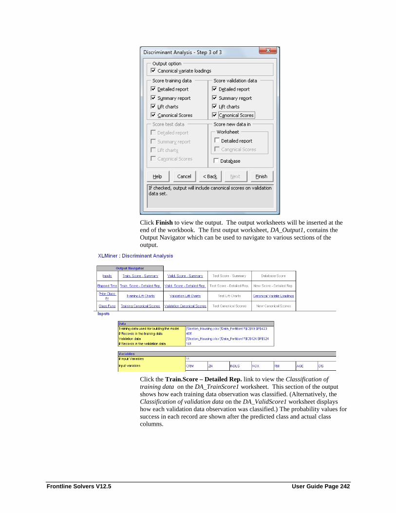
Frontline Solvers V12.5 User Guide Page 242
Click Finish to view the output. The output worksheets will be inserted at the
end of the workbook. The first output worksheet, DA_Output1, contains the
Output Navigator which can be used to navigate to various sections of the
output.
Click the Train.Score – Detailed Rep. link to view the Classification of
training data on the DA_TrainScore1 worksheet. This section of the output
shows how each training data observation was classified. (Alternatively, the
Classification of validation data on the DA_ValidScore1 worksheet displays
how each validation data observation was classified.) The probability values for
success in each record are shown after the predicted class and actual class
columns.

Frontline Solvers V12.5 User Guide Page 243
Click the Class Funs link to view the Classification Function table. In this
example, there are 2 functions -- one for each class. Each variable is assigned to
the class that contains the higher value.
Click the Canonical Variate Loadings link to navigate to the Canonical
Variate Loadings section.
Canonical Variate Loadings are a second set of functions that give a
representation of the data that maximizes the separation between the classes.
The number of functions is one less than the number of classes (so in this case
there is one function). If we were to plot the cases in this example on a line
where xi is the ith case's value for variate1, you would see a clear separation of
the data. This output is useful in illustrating the inner workings of the
discriminant analysis procedure, but is not typically needed by the end-user
analyst.

Frontline Solvers V12.5 User Guide Page 244
Click the Training Lift Charts link to navigate to the Training Data Lift Charts.
In a Lift Chart, the x axis is the cumulative number of cases and the y axis is the
cumulative number of true positives. The red line originating from the origin
and connecting to the point (400, 65) is a reference line that represents the
expected number of CAT MEDV predictions if XLMiner simply selected
random cases – i.e. no model was used. This reference line provides a yardstick
against which the user can compare the model performance. From the Lift Chart
below we can infer that if we assigned 200 cases to class 1, 62 1’s would be
included. If 200 cases were selected at random, we could expect 33 1’s (200 *
65/400 = 32.5).
Click the Training Canonical Scores link to navigate to the DA_TrainCanSco1
worksheet. Canonical Scores are the values of each case for the function. Again,
these are intermediate values useful for illustration but not required by the end-
user analyst.

Frontline Solvers V12.5 User Guide Page 245
For information on Stored Model Sheets, in this example DA_Stored_1, please
refer to the Scoring chapter.
Discriminant Analysis Options The options below appear on the Discriminant Analysis dialogs.

Frontline Solvers V12.5 User Guide Page 246
Variables in input data
The variables present in the dataset are listed here.
Input variables
The variables to be included in the Discriminant Analysis algorithm are listed
here.
Weight Variables
This option is not used for Discriminant Analysis.
Output variable
The selected output variable is displayed here. XLMiner supports a maximum
of 30 classes in the output variable.
#Classes
This value is the number of classes in the output variable.
Specify “Success” class (for Lift Chart)
This option is selected by default. Select the class to be considered a “success”
or the significant class in the Lift Chart. This option is enabled when the
number of classes in the output variable is equal to 2.
Specify initial cutoff probability value for success
Enter a value between 0 and 1 here to denote the cutoff probability for success.
If the calculated probability for success for an observation is greater than or
equal to this value, than a “success” (or a 1) will be predicted for that
observation. If the calculated probability for success for an observation is less
than this value, then a “non-success” (or a 0) will be predicted for that
observation. The default value is 0.5. This option is only enabled when the # of
classes is equal to 2.
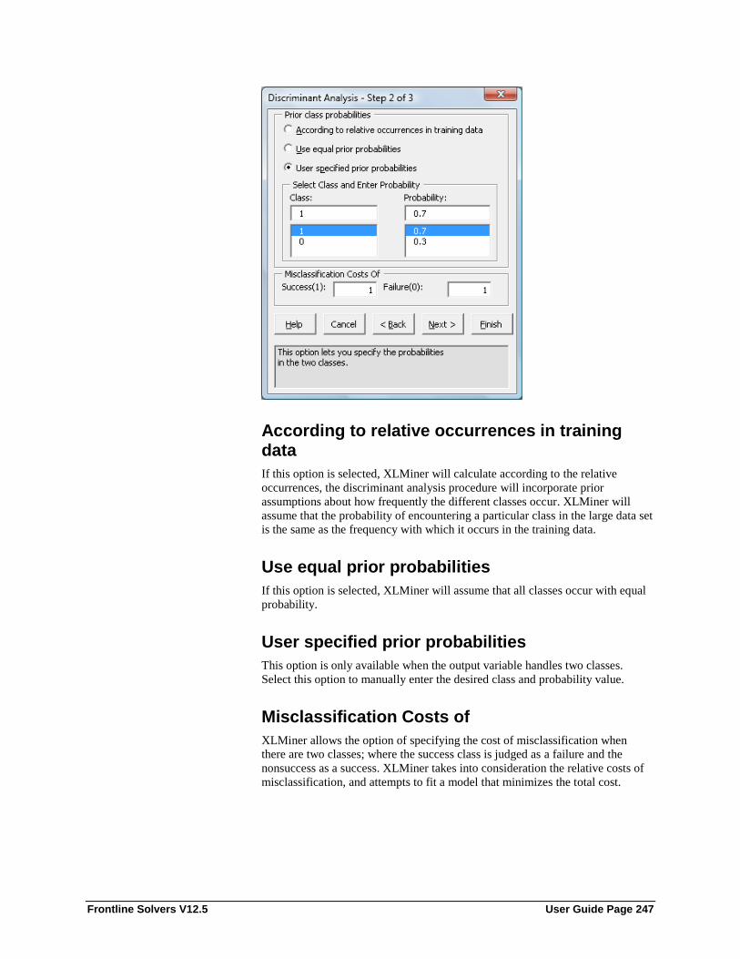
Frontline Solvers V12.5 User Guide Page 247
According to relative occurrences in training data
If this option is selected, XLMiner will calculate according to the relative
occurrences, the discriminant analysis procedure will incorporate prior
assumptions about how frequently the different classes occur. XLMiner will
assume that the probability of encountering a particular class in the large data set
is the same as the frequency with which it occurs in the training data.
Use equal prior probabilities
If this option is selected, XLMiner will assume that all classes occur with equal
probability.
User specified prior probabilities
This option is only available when the output variable handles two classes.
Select this option to manually enter the desired class and probability value.
Misclassification Costs of
XLMiner allows the option of specifying the cost of misclassification when
there are two classes; where the success class is judged as a failure and the
nonsuccess as a success. XLMiner takes into consideration the relative costs of
misclassification, and attempts to fit a model that minimizes the total cost.

Frontline Solvers V12.5 User Guide Page 248
Canonical variate loadings
When this option is selected, XLMiner produces the canonical variates for the
data based on an orthogonal representation of the original variates. This has the
effect of choosing a representation which maximizes the distance between the
different groups. For a k class problem there are k-1 Canonical variates.
Typically, only a subset of the canonical variates is sufficient to discriminate
between the classes. For this example, we have two canonical variates which
means that if we replace the four original predictors by just two predictors, X1
and X2, (which are actually linear combinations of the four original predictors)
the discrimination based on these two predictors will perform just as well as the
discrimination based on the original predictors.
Score training data
Select these options to show an assessment of the performance of the tree in
classifying the training data. The report is displayed according to your
specifications - Detailed, Summary and Lift charts.
Score validation data
Select these options to show an assessment of the performance of the tree in
classifying the validation data. The report is displayed according to your
specifications - Detailed, Summary and Lift charts.
Score test data
These options are enabled when a test set is present. Select these options to
show an assessment of the performance of the tree in classifying the test data.
The report is displayed according to your specifications - Detailed, Summary
and Lift charts.

Frontline Solvers V12.5 User Guide Page 249
Canonical Scores
The values of the variables X1 and X2 for the ith
observation are known as the
canonical scores for that observation. In this example, the pair of canonical
scores for each observation represents the observation in a two dimensional
space. The purpose of the canonical score is to separate the classes as much as
possible. Thus, when the observations are plotted with the canonical scores as
the coordinates, the observations belonging to the same class are grouped
together. When this option is selected for either the Training, Validation or Test
sets, XLMiner reports the scores of the first few observations.
See the Scoring chapter for more information on the options located in the Score
Test Data and Score New Data groups.

Frontline Solvers V12.5 User Guide Page 250
Logistic Regression
Introduction Logistic regression is a variation of ordinary regression which is used when the
dependent (response) variable is a dichotomous variable. A dichotomous
variable takes only two values, which typically represent the occurrence or non-
occurrence of some outcome event and are usually coded as 0 or 1 (success).
The independent (input) variables are continuous, categorical, or both. An
example of a categorical variable in a medical study would be a patient’s status
after five years - the patient can either survive (1) or die (0).
Unlike ordinary linear regression, logistic regression does not assume that the
relationship between the independent variables and the dependent variable is a
linear one. Nor does it assume that the dependent variable or the error terms are
distributed normally.
The form of the model is
where p is the probability that Y=1 and X1, X2,.. .,Xk are the independent
variables (predictors). b0 , b1, b2, .... bk are known as the regression coefficients,
which have to be estimated from the data. Logistic regression estimates the
probability of a certain event occurring.
Logistic regression thus forms a predictor variable (log (p/(1-p)) which is a
linear combination of the explanatory variables. The values of this predictor
variable are then transformed into probabilities by a logistic function. Such a
function has the shape of an S. On the horizontal axis we have the values of the
predictor variable, and on the vertical axis we have the probabilities.

Frontline Solvers V12.5 User Guide Page 251
Logistic regression also produces Odds Ratios (O.R.) associated with each
predictor value. The "odds" of an event is defined as the probability of the
outcome event occurring divided by the probability of the event not occurring.
In general, the "odds ratio" is one set of odds divided by another. The odds ratio
for a predictor is defined as the relative amount by which the odds of the
outcome increase (O.R. greater than 1.0) or decrease (O.R. less than 1.0) when
the value of the predictor variable is increased by 1.0 units. In other words,
(odds for PV+1)/(odds for PV) where PV is the value of the predictor variable.
Logistic Regression Example This example illustrates XLMiner’s Logistic Regression algorithm. Click Help
– Examples on the XLMiner ribbon and open the example file,
Charles_Bookclub.xlsx. This file contains information associated with
individuals who are members of a book club. This example develops a model
for predicting whether a person will purchase a book about the city of Florence
based on previous purchases.
First, we partition the data using a standard partition with percentages of 70%
training and 30% validation. (For more information on how to partition a
dataset, please see the previous Data Mining Partitioning chapter.)

Frontline Solvers V12.5 User Guide Page 252
Select a cell on the Data_Partition1 output worksheet, then click Classify –
Logistic Regression on the XLMiner ribbon. The Logistic Regression dialog
appears.

Frontline Solvers V12.5 User Guide Page 253
Since we are interested in predicting if a customer will purchase a book about
the city of Florence, we will choose Florence as our output variable. In the
dataset, if a customer purchased a book about the city of Florence, the variable
value equals 1. If a customer did not purchase a book about the city of Florence,
the value equals 0.
Select all remaining variables except Seq# and ID# as Input variables. These
two variables are unique identifiers and should not be included as neither have
any significance in the classification method.

Frontline Solvers V12.5 User Guide Page 254
Choose the value that will be the indicator of “Success” by clicking the down
arrow next to Specify “Success” class (necessary). In this example, we will use
the default of 1.
Enter a value between 0 and 1 for Specify the initial cutoff probability for
success. If the Probability of success (probability of the output variable = 1) is
less than this value, then a 0 will be entered for the class value, otherwise a 1
will be entered for the class value. In this example, we will keep the default of
0.5.
Click Next to advance to Step 2 of 3 of the Logistic Regression algorithm.
Selecting Set confidence level for odds alters the level of confidence for the
confidence levels displayed in the results for the odds ratio.
Selecting Force constant term to zero omits the constant term in the regression.
For this example, select Set confidence level for odds leaving the percentage at
95%.

Frontline Solvers V12.5 User Guide Page 255
Click Advanced… The following dialog opens.
Keep the default of 50 for the Maximum # iterations. Estimating the coefficients
in the Logistic Regression algorithm requires an iterative non-linear
maximization procedure. You can specify a maximum number of iterations to
prevent the program from getting lost in very lengthy iterative loops. This value
must be an integer greater than 0 or less than or equal to 100 (1< value <= 100).
Keep the default of 1 for the Initial marquardt overshoot factor. This overshoot
factor is used in the iterative non-linear maximization procedure. Reducing this
value speeds the operation by reducing the number of iterations required but
increases the chances that the maximization procedure will fail due to overshoot.
This value must be an integer greater than 0 or less than or equal to 50 (0 <
value <=50).
At times, variables can be highly correlated with one another which can result in
large standard errors for the affected coefficients. XLMiner will display
information useful in dealing with this problem if Perform Collinearity
diagnostics is selected. For this example, select Perform Collinearity
diagnostics and enter 2 for the Number of collinearity components. This option
can take on integer values from 2 to 15 (2 <= value <= 15).

Frontline Solvers V12.5 User Guide Page 256
Click OK to return to the Step 2 of 3 dialog, then click Best subset…
Select Perform best subset selection. Often a subset of variables (rather than
all of the variables) performs the best job of classification. Selecting Perform
best subset selection enables the Best Subset options.
Using the spinner controls, specify 15 for the Maximum size of best subset. It’s
possible that XLMiner could find a smaller subset of variables. This option can
take on values of 1 up to N where N is the number of input variables. The
default setting is 15.
Using the spinner controls, specify 15 for the Number of best subsets. XLMiner
can provide up to 20 different subsets. The default setting is 1.
XLMiner offers five different selection procedures for selecting the best subset
of variables.
Backward elimination in which variables are eliminated one at a time,
starting with the least significant.
Forward selection in which variables are added one at a time, starting
with the most significant.
Exhaustive search where searches of all combinations of variables are
performed to observe which combination has the best fit. (This option
can become quite time consuming depending on the number of input
variables.)

Frontline Solvers V12.5 User Guide Page 257
Sequential replacement in which variables are sequentially replaced
and replacements that improve performance are retained.
Stepwise selection is similar to Forward selection except that at each
stage, XLMiner considers dropping variables that are not statistically
significant. When this procedure is selected, the Stepwise selection
options FIN and FOUT are enabled. In the stepwise selection
procedure a statistic is calculated when variables are added or
eliminated. For a variable to come into the regression, the statistic’s
value must be greater than the value for FIN (default = 3.84). For a
variable to leave the regression, the statistic’s value must be less than
the value of FOUT (default = 2.71). The value for FIN must be greater
than the value for FOUT.
For this example, select Backward elimination.
Click OK to return to the Step 2 of 3 dialog. Click Next to advance to the Step 3
of 3 dialog.

Frontline Solvers V12.5 User Guide Page 258
Select Covariance matrix of coefficieints. When this option is selected,
XLMiner will display the coefficient covariance matrix in the output. Entries in
the matrix are the covariances between the indicated coefficients. The “on-
diagonal” values are the estimated variances of the corresponding coefficients.
Select Residuals. When this option is selected, XLMiner will produce a two-
column array of fitted values and their residuals in the output.
Select Detailed report under both Score training data and Score validation
data. XLMiner will create a detailed report, complete with an Output
Navigator, for ease in routing to specific areas in the output worksheets.
Select Summary report under both Score training data and Score validation
data. XLMiner will create a report that summarizes the regression output for
both datasets.
Select Lift charts under both Score training data and Score validation data.
XLMiner will create a lift chart for both datasets.
For information on scoring in a worksheet or database, please see the Scoring
chapter.

Frontline Solvers V12.5 User Guide Page 259
Click Finish. The logistic regression output worksheets are inserted at the end
of the workbook. Use the Output Navigator on the first output worksheet,
LR_Output 1.
A number of sections of output are available, including Classification of the
Training Data as shown below. Note that XLMiner has not, strictly speaking,
classified the data -- it has assigned a "predicted probability of success" to each
case. This is the predicted probability, based on the input (independent) variable
values for a case, that the output (dependent) variable for the case will be a "1".
Since the logistic regression procedure works not with the actual values of the
variable but with the logs of the odds ratios, this value is shown in the output
(the predicted probability of success is derived from it).
To classify each record as a "1" or a "0," we would simply assign a "1" to the
record if the predicted probability of success exceeds a certain value. In this
example the initial cutoff probability was set to 0.5 on the first Logistic
Regression dialog. A value of "0" will be assigned if the prediction probability
of success is less than the cutoff probability.

Frontline Solvers V12.5 User Guide Page 260
Since we selected Perform best subset selection on the Best Subset dialog,
XLMiner has produced the following output which displays the variables that
are included in the subsets. Since we selected 15 as the size of the subset, we are
shown the best subset of 1 variable (plus the constant), up to the best subset for
15 variables (plus the constant). This list comprises several different models
XLMiner generated using the Backward Elimination Selection Procedure as
chosen on the Best Subset dialog.
Refer to the Best Subset output above. In this section, every model includes a
constant term (since Force constant term to zero was not selected in Step 2 of 2)
and one or more variables as the additional coefficients. We can use any of these
models for further analysis by clicking on the respective link Choose Subset.
The choice of model depends on the calculated values of various error values
and the probability. RSS is the residual sum of squares, or the sum of squared
deviations between the predicted probability of success and the actual value (1
or 0). Cp is "Mallows Cp" and is a measure of the error in the best subset model,
relative to the error incorporating all variables. Adequate models are those for
which Cp is roughly equal to the number of parameters in the model (including
the constant), and/or Cp is at a minimum. "Probability" is a quasi hypothesis test
of the proposition that a given subset is acceptable; if Probability < .05 we can
rule out that subset.
When hoving over Choose Subset, the mouse icon will change to a “grabber
hand”. If Choose Subset is clicked, XLMiner opens the Logistic Regression
Step 1 of 1 dialog displaying the input variables included in that particular
subset. Scroll down to the end of the table.
The considerations about RSS, Cp and Probability would lead us to believe that
the subsets with 10 or 11 coefficients are the best models in this example.
Model terms are shown in the Regression Model output shown below.

Frontline Solvers V12.5 User Guide Page 261
This table contains the coefficient, the standard error of the coefficient, the p-
value and the odds ratio for each variable (which is simply ex where x is the
value of the coefficient) and confidence interval for the odds.
Summary statistics to the right (above) show the residual degrees of freedom
(#observations - #predictors), a standard deviation type measure for the model
(which typically has a chi-square distribution), the percentage of successes (1's)
in the training data, the number of iterations required to fit the model, and the
Multiple R-squared value.
The multiple R-squared value shown here is the r-squared value for a logistic
regression model , defined as -
R2 = (D0-D)/D0 ,
where D is the Deviance based on the fitted model and D0 is the deviance based
on the null model. The null model is defined as the model containing no
predictor variables apart from the constant.
Collinearity Diagnostics help assess whether two or more variables so closely
track one another as to provide essentially the same information.

Frontline Solvers V12.5 User Guide Page 262
The columns represent the variance components (related to principal
components in multivariate analysis), while the rows represent the variance
proportion decomposition explained by each variable in the model. The
eigenvalues are those associated with the singular value decomposition of the
variance-covariance matrix of the coefficients, while the condition numbers are
the ratios of the square root of the largest eigenvalue to all the rest. In general,
multicollinearity is likely to be a problem with a high condition number (more
than 20 or 30), and high variance decomposition proportions (say more than 0.5)
for two or more variables.
Lift charts (on the LR_TrainLiftChart and LR_ValidLiftChart, respectively) are
visual aids for measuring model performance. They consist of a lift curve and a
baseline. The greater the area between the lift curve and the baseline, the better
the model.

Frontline Solvers V12.5 User Guide Page 263
After the model is built using the training data set, the model is used to score on
the training data set and the validation data set (if one exists). Then the data
set(s) are sorted using the predicted output variable value (or predicted
probability of success in the logistic regression case). After sorting, the actual
outcome values of the output variable are cumulated and the lift curve is drawn
as the number of cases versus the cumulated value. The baseline (red line
connecting the origin to the end point of the blue line) is drawn as the number of
cases versus the average of actual output variable values multiplied by the
number of cases. The decilewise lift curve is drawn as the decile number versus
the cumulative actual output variable value divided by the decile's average
output variable value.
See the chapter on Stored Model Sheets for more information on the
LR_Stored_1 worksheet.
Logistic Regression Options The following options appear on one of the five Logistic Regression dialogs.

Frontline Solvers V12.5 User Guide Page 264
Variables in input data
All variables in the dataset are listed here.
Input variables
Variables listed here will be utilized in the XLMiner output.
Weight variable
One major assumption of Logistic Regression is that each observation provides
equal information. XLMiner offers an opportunity to provide a Weight variable.
Using a Weight variable allows the user to allocate a weight to each record. A
record with a large weight will influence the model more than a record with a
smaller weight.
Output Variable
Select the variable whose outcome is to be predicted.
# Classes
Displays the number of classes in the Output variable.

Frontline Solvers V12.5 User Guide Page 265
Specify “Success” class (necessary) This option is selected by default. Select the class to be considered a “success”
or the significant class in the Lift Chart. This option is enabled when the
number of classes in the output variable is equal to 2Specify initial cutoff
probability value for success.
Specify initial Cutoff Probability value for success
Enter a value between 0 and 1 here to denote the cutoff probability for success.
If the calculated probability for success for an observation is greater than or
equal to this value, than a “success” (or a 1) will be predicted for that
observation. If the calculated probability for success for an observation is less
than this value, then a “non-success” (or a 0) will be predicted for that
observation. The default value is 0.5. This option is only enabled when the # of
classes is equal to 2.
Force constant term to zero
Select this option to omit the constant term in the regression
Set confidence level for odds
Select this option to alter the level of confidence for the confidence levels
displayed in the results for the odds ratio.

Frontline Solvers V12.5 User Guide Page 266
Maximum # iterations
Estimating the coefficients in the Logistic Regression algorithm requires an
iterative non-linear maximization procedure. You can specify a maximum
number of iterations to prevent the program from getting lost in very lengthy
iterative loops. This value must be an integer greater than 0 or less than or equal
to 100 (1< value <= 100). The default value is 50.
Initial marquardt overshoot factor
This overshoot factor is used in the iterative non-linear maximization procedure.
Reducing this value speeds the operation by reducing the number of iterations
required but increases the chances that the maximiation procedure will fail due
to overshoot. This value must be an integer greater than 0 or less than or equal
to 50 (0 < value <=50). The default value is 1.
Perform Collinearity diagnostics
At times, variables can be highly correlated with one another which can result in
large standard errors for the affected coefficients. XLMiner will display
information useful in dealing with this problem if Perform Collinearity
diagnostics is selected. This option is not selected by default.
Number of collinearity components
This option is enabled when Perform Collinearity diagnostics is selected and
determines the number of collinearity components included in the Collinearity
diagnostic output. Enter an integer value greater than or equal to 2 and less than
or equal to the number of predictors in the model (input variables) (2 <= value
<= Number of predictors (input variables)). The default value is the number of
predictors (or input variables) included in the model.
Perform best subset selection
Often a subset of variables (rather than all of the variables) performs the best job
of classification. Selecting Perform best subset selection enables the Best
Subset options. This option is not selected by default.

Frontline Solvers V12.5 User Guide Page 267
Maximum size of best subset
Use the spinner controls to specify the number of best subsets generated by
XLMiner. It’s possible that XLMiner could find a smaller subset of variables.
This option can take on values of 1 up to N where N is the number of input
variables. The default setting is 15.
Number of best subsets
Using the spinner controls, specify the Number of best subsets. XLMiner can
provide up to 20 different subsets. The default setting is 1.
Selection Procedure
XLMiner offers five different selection procedures for selecting the best subset
of variables.
Backward elimination in which variables are eliminated one at a time,
starting with the least significant.
Forward selection in which variables are added one at a time, starting
with the most significant.
Exhaustive search where searches of all combinations of variables are
performed to observe which combination has the best fit. (This option
can become quite time consuming depending on the number of input
variables.)
Sequential replacement in which variables are sequentially replaced
and replacements that improve performance are retained.
Stepwise selection is similar to Forward selection except that at each
stage, XLMiner considers dropping variables that are not statistically
significant. When this procedure is selected, the Stepwise selection
options FIN and FOUT are enabled.
In the stepwise selection procedure a statistic is calculated when
variables are added or eliminated. For a variable to come into the
regression, the statistic’s value must be greater than the value for FIN
(default = 3.84). For a variable to leave the regression, the statistic’s
value must be less than the value of FOUT (default = 2.71). The value
for FIN must be greater than the value for FOUT.

Frontline Solvers V12.5 User Guide Page 268
Covariance matrix of coefficients
When this option is selected, XLMiner will display the coefficient covariance
matrix in the output. Entries in the matrix are the covariances between the
indicated coefficients. The “on-diagonal” values are the estimated variances of
the corresponding coefficients.
Residuals
When this option is selected, XLMiner will produce a two-column array of fitted
values and their residuals in the output.
Score training data
Select these options to show an assessment of the performance of the tree in
classifying the training data. The report is displayed according to your
specifications - Detailed, Summary and Lift charts.
Score validation data
Select these options to show an assessment of the performance of the tree in
classifying the validation data. The report is displayed according to your
specifications - Detailed, Summary and Lift charts.
Score test data
These options are enabled when a test set is present. Select these options to
show an assessment of the performance of the tree in classifying the test data.
The report is displayed according to your specifications - Detailed, Summary
and Lift charts.

Frontline Solvers V12.5 User Guide Page 269
Score new data
For information on scoring in a worksheet or database, please see the Scoring
chapter.

Frontline Solvers V12.5 User Guide Page 270
k – Nearest Neighbors Classification Method
Introduction In the k-nearest-neighbor classification method, the training dataset is used to
classify each member of a "target" dataset. The structure of the data is that there
is a classification (categorical) variable ("buyer," or "non-buyer," for example),
and a number of additional predictor variables (age, income, location, etc.).
1. For each row (case) in the target dataset (the set to be classified), the k
closest members (the k nearest neighbors) of the training dataset are located.
A Euclidean Distance measure is used to calculate how close each member
of the training set is to the target row that is being examined.
2. Examine the k nearest neighbors - which classification (category) do most
of them belong to? Assign this category to the row being examined.
3. Repeat this procedure for the remaining rows (cases) in the target set.
4. XLMiner allows the user to select a maximum value for k and builds
models in parallel on all values of k up to the maximum specified value.
Additional scoring can be performed on the best of these models.
As k increases, the computing time increases. However a larger k will reduce
the vulnerability of the training data to outside variability which might offset the
increased time requirement. In most applications, k is in units of tens rather than
in hundreds or thousands.
k-Nearest Neighbors Classification Example The example below illustrates’ the use of XLMiner’s k-Nearest Neighbors
classification method. Click Help – Examples on the XLMiner ribbon and
open the example dataset Iris.xlsx. This dataset was introduced by R. A. Fisher
and reports four characteristics of three species of the Iris flower.

Frontline Solvers V12.5 User Guide Page 271
First, we partition the data using a standard partition with percentages of 60%
training and 40% validation (the default settings for the Automatic choice).
For more information on how to partition a dataset, please see the previous Data
Mining Partitioning chapter.
Select a cell on the Data_Partition1 worksheet, then click Classify – k-Nearest
Neighbors on the XLMiner ribbon to open the k-Nearest Neighbors Step 1 of 2
dialog, as shown below.

Frontline Solvers V12.5 User Guide Page 272
Select Petal_width, Petal_length, Sepal_width, and Sepal_length under
Variables in input data then click > to select as input variables. Select
Species_name as the output variable or the variable to be classified. Once the
Output variable is selected, # Classes (3) will be filled automatically. Since our
output variable contains more than 2 classes, Specify “Success” class and
Specify initial cutoff value fields are disabled.

Frontline Solvers V12.5 User Guide Page 273
Click OK to advance to Step 2 of 2.
Select Normalize input data. When this option is selected, XLMiner will
normalize the data by expressing the entire dataset in terms of standard
deviations. This is done so that the distance measure is not dominated by a large

Frontline Solvers V12.5 User Guide Page 274
magnitude variable. In this example, the values for Petal_width are between .1
and 2.5 while the values for Sepal_length are between 4.3 and 7.9. When the
data is normalized the actual variable value (say 4.3) is replaced with the
standard deviation from the mean of that variable. This option is not selected by
default.
Enter 10 for Number of nearest neighbors (k). (This number is based on
standard practice from the literature.) This is the parameter k in the k-Nearest
Neighbor algorithm. The value of k should be between 1 and the total number
of observations (rows). Note that if k is chosen as the total number of
observations in the training set, then for any new observation, all the
observations in the training set become nearest neighbors. The default value for
this option is 1.
Select Score on best k between 1 and specified value under Scoring option.
When this option is selected, XLMiner will display the output for the best k
between 1 and the value entered for Number of nearest neighbors (k). If Score
on specified value of k as above is selected, the output will be displayed for the
specified value of k.
Select Detailed scoring and Summary report under both Score training data
and Score validation data. XLMiner will create detailed and summary reports
for both the training and validation sets.
For more information on the Score new data options, please see the Scoring
chapter.
Click Finish. Click the KNNC_Output1 worksheet, the Output Navigator is
located at the top of this worksheet. Clink the links to navigate to other areas of

Frontline Solvers V12.5 User Guide Page 275
the output. Scroll down on the Output1 worksheet to view the Validation error
log.
The Validation error log for the different k's lists the % Errors for all values of k
for both the training and validation data sets. The k with the smallest % Error is
selected as the “Best k”. Scoring is performed later using this best value of k.
A little further down on the Output1 worksheet, is the Validation Data scoring
table.
This Summary report tallies the actual and predicted classifications. (Predicted
classifications were generated by applying the model to the validation data.)
Correct classification counts are along the diagonal from the upper left to the
lower right. In this example, there were three misclassification errors (3 cases
where Verginicas were misclassified as Versicolors).
Click the Valid. Score – Detailed Rep. link on the Output Navigator to be
routed to the ValidScore1 worksheet.
This table shows the predicted class for each record, the percent of the nearest
neighbors belonging to that class and the actual class. The class with the highest
probability is highlighted in yellow. Mismatches between Predicted and Actual
class are highlighted in green.

Frontline Solvers V12.5 User Guide Page 276
Scroll down to view record 107 which is one of the three misclassified records.
The additional two misclassified records are 120 and 134.
k-Nearest Neighbors Options The following options appear on one of the two k-Nearest Neighbors dialogs.

Frontline Solvers V12.5 User Guide Page 277
Variables in input data
The variables in the dataset appear here.
Input variables
The variables selected as input variables appear here
Weight variable
This option is not used in the k-Nearest Neighbors classification method.
Output variable
The variable to be classified is entered here.
Classes in the output variable
The number of classes in the output variable appear here.
Specify Success class (for Lift Charts) This option is selected by default. Select the class to be considered a “success”
or the significant class in the Lift Chart. This option is enabled when the
number of classes in the output variable is equal to 2Specify initial cutoff
probability value for success.

Frontline Solvers V12.5 User Guide Page 278
Specify Initial Cutoff Probability value for success
Enter a value between 0 and 1 here to denote the cutoff probability for success.
If the calculated probability for success for an observation is greater than or
equal to this value, than a “success” (or a 1) will be predicted for that
observation. If the calculated probability for success for an observation is less
than this value, then a “non-success” (or a 0) will be predicted for that
observation. The default value is 0.5. This option is only enabled when the # of
classes is equal to 2.
Normalize input data
When this option is selected, XLMiner will normalize the data by expressing the
entire dataset in terms of standard deviations. This is done so that the distance
measure is not dominated by a large magnitude variable. In this example, the
values for Petal_width are between .1 and 2.5 while the values for Sepal_length
are between 4.3 and 7.9. When the data is normalized the actual variable value
is replaced with the standard deviation from the mean of that variable.
Number of nearest neighbors (k)
This is the parameter k in the k-Nearest Neighbor algorithm. The value of k
should be between 1 and the total number of observations (rows). Note that if k
is chosen as the total number of observations in the training set, then for any
new observation, all the observations in the training set become nearest
neighbors. The default value for this option is 1.

Frontline Solvers V12.5 User Guide Page 279
Scoring Option
If Score on best k between 1 and specified value is selected, XLMiner will
display the output for the best k between 1 and the value entered for Number of
nearest neighbors (k).
If Score on specified value of k as above is selected, the output will be displayed
for the specified value of k.
Score training data
Select these options to show an assessment of the performance of the tree in
classifying the training data. The report is displayed according to your
specifications - Detailed, Summary and Lift charts.
Score validation data
Select these options to show an assessment of the performance of the tree in
classifying the validation data. The report is displayed according to your
specifications - Detailed, Summary and Lift charts.
Score test data
These options are enabled when a test set is present. Select these options to
show an assessment of the performance of the tree in classifying the test data.
The report is displayed according to your specifications - Detailed, Summary
and Lift charts.
Score new data
For more information on the Score new data options, please see the Scoring
chapter.

Frontline Solvers V12.5 User Guide Page 280
Classification Tree Classification Method
Introduction Classification tree methods (also known as decision tree methods) are a good
choice when the data mining task is classification or prediction of outcomes and
the goal is to generate rules that can be easily understood, explained, and
translated into SQL or a natural query language.
A Classification tree labels, records and assigns variables to discrete classes. A
Classification tree can also provide a measure of confidence that the
classification is correct.
A Classification tree is built through a process known as binary recursive
partitioning. This is an iterative process of splitting the data into partitions, and
then splitting it up further on each of the branches.
Initially, a training set is created where the classification label (say, "purchaser"
or "non-purchaser") is known (pre-classified) for each record. In the next step,
the algorithm systematically assigns each record to one of two subsets on the
some basis, for example income > $75,000 or income <= $75,000). The object is
to attain as homogeneous set of labels (say, "purchaser" or "non-purchaser") as
possible in each partition. This splitting (or partitioning) is then applied to each
of the new partitions. The process continues until no more useful splits can be
found. The heart of the algorithm is the rule that determines the initial split rule
(see figure below).

Frontline Solvers V12.5 User Guide Page 281
As explained above, the process starts with a training set consisting of pre-
classified records (target field or dependent variable with a known class or label
such as "purchaser" or "non-purchaser"). The goal is to build a tree that
distinguishes among the classes. For simplicity, assume that there are only two
target classes and that each split is a binary partition. The splitting criterion
easily generalizes to multiple classes, and any multi-way partitioning can be
achieved through repeated binary splits. To choose the best splitter at a node, the
algorithm considers each input field in turn. In essence, each field is sorted.
Then, every possible split is tried and considered, and the best split is the one
which produces the largest decrease in diversity of the classification label within
each partition (this is just another way of saying "the increase in homogeneity").
This is repeated for all fields, and the winner is chosen as the best splitter for
that node. The process is continued at subsequent nodes until a full tree is
generated.
XLMiner uses a modified “twoing splitting rule”, as described on page 316 of
Classification and Regression Trees by Breiman, et al (1984, Chapman and
Hall). Please refer to this book for details. It maximizes the value of Ø which is
calculated as given in the last formula on this page:
Pruning the tree
Pruning is the process of removing leaves and branches to improve the
performance of the decision tree when moving from the training data (where the
classification is known) to real-world applications (where the classification is
unknown). The tree-building algorithm makes the best split at the root node
where there are the largest number of records and, hence, considerable
information. Each subsequent split has a smaller and less representative
population with which to work. Towards the end, idiosyncrasies of training
records at a particular node display patterns that are peculiar only to those
records. These patterns can become meaningless and sometimes harmful for
prediction if you try to extend rules based on them to larger populations.
For example, say the classification tree is trying to predict height and it comes to
a node containing one tall person X and several other shorter people. The
algorithm can decrease diversity at that node by a new rule imposing "people
named X are tall" and thus classify the training data. In the real world this rule is
obviously inappropriate. Pruning methods solve this problem -- they let the tree
grow to maximum size, then remove smaller branches that fail to generalize.
(Note: In practice, we do not include irrelevant fields such as "name", this is
simply used an illustration.)
Since the tree is “grown” from the training data set, when it has reached full
structure it usually suffers from over-fitting (i.e. it is "explaining" random
elements of the training data that are not likely to be features of the larger
population of data). This results in poor performance on real life data.
Therefore, trees must be pruned using the validation data set.
Classification Tree Example This example illustrates the use of XLMiner’s Classification Tree algorithm on
the Boston_Housing.xlsx dataset.

Frontline Solvers V12.5 User Guide Page 282
Click Help – Examples to open the Boston_Housing.xlsx dataset. This dataset
includes fourteen variables pertaining to hosing prices from the Boston area
collected by the US Census Bureau.
CRIM Per capita crime rate by town ZN Proportion of residential land zoned for lots over 25,000 sq.ft. INDUS Proportion of non-retail business acres per town CHAS Charles River dummy variable (= 1 if tract bounds river; 0 otherwise) NOX Nitric oxides concentration (parts per 10 million) RM Average number of rooms per dwelling AGE Proportion of owner-occupied units built prior to 1940
DIS Weighted distances to five Boston employment centers RAD Index of accessibility to radial highways TAX Full-value property-tax rate per $10,000 PTRATIO Pupil-teacher ratio by town B 1000(Bk - 0.63)^2 where Bk is the proportion of African-Americans by
town LSTAT % Lower status of the population MEDV Median value of owner-occupied homes in $1000's
The figure below displays a portion of the data; observe the last column (CAT.
MEDV). This variable has been derived from the MEDV variable by assigning
a 1 for MEDV levels above 30 (>= 30) and a 0 for levels below 30 (<30).
First, we partition the data into training and validation sets using the Standard
Data Partition defaults of 60% of the data randomly allocated to the Training Set
and 40% of the data randomly allocated to the Validation Set. For more
information on partitioning a dataset, see the Data Mining Partitioning chapter.

Frontline Solvers V12.5 User Guide Page 283
Select a cell on the Data_Partition1 worksheet, inserted after clicking OK on
the Standard Data Partition dialog above, then click Classify – Classification
Tree on the XLMiner ribbon. The following dialog opens.

Frontline Solvers V12.5 User Guide Page 284
Select CAT. MEDV as the Output variable. Then select all remaining
variables except MEDV as Input variables. The MEDV variable is not
included in the Input since the CAT. MEDV variable is derived from the MEDV
variable.
Keep the default settings for Specify “Success” class and Specify initial cutoff
probability.

Frontline Solvers V12.5 User Guide Page 285
Click Next to advance to the Step 2 of 3 dialog.
In the Classification Tree Step 2 of 3 dialog, select Normalize input data,
Minimum #records in a terminal node, and Prune tree. Enter 2 for Minimum
#records in a terminal node.
XLMiner will normalize the data when Normalize input data is selected.
Normalization helps only if linear combinations of the input variables are used
when splitting the tree.
Select Minimum #records in a terminal node to stop the training data as soon
as the number of records in a node reaches the specified minimum value. Enter
2 for the minimum value. The default value is 30.
XLMiner will prune the tree using the validation set when Prune Tree is
selected. (Pruning the tree using the validation set will reduce the error from
over-fitting the tree using the training data.)

Frontline Solvers V12.5 User Guide Page 286
Click Next to advance to the Step 3 of 3 dialog.
XLMiner provides the option to provide maximum #levels in the tree. Set
Maximum # levels to be displayed to 4 to indicate to XLMiner only four levels
in the tree are desired.
Select Full tree (grown using training data) to “grow” a complete tree using
the training data.
Select Best pruned tree (pruned using validation data). Selecting this option
will result in a tree with the fewest number of nodes, subject to the constraint
that the error be kept below a specified level (minimum error rate plus the
standard error of that error rate).
Select Minimum error tree (pruned using validation data) to produce a tree
that yields the minimum classification error rate when tested on the validation
data.

Frontline Solvers V12.5 User Guide Page 287
To create a tree with a specified number of decision nodes select Tree with
specified number of decision nodes and enter the desired number of nodes.
Leave this option unselected for this example.
Select the three options under both Score training data and Score validation
data to produce an assessment of the performance of the tree in both sets.
Please see the Scoring chapter for information on the Score new data options.
Click Finish. Worksheets containing the output of the Classification Tree
algorithm will be inserted at the end of the workbook. Click the CT_Output1
worksheet to view the Output Navigator. Click any link in this section to
navigate to various sections of the output.

Frontline Solvers V12.5 User Guide Page 288
Click the CT_FullTree1 worksheet tab to view the full tree.
Recall that the objective of this example is to classify each case as a 0 (low
median value) or a 1 (high median value). Consider the top decision node
(denoted by a circle). The label beneath this node indicates the variable
represented at this node (i.e. the variable selected for the first split) in this case,
RM = average number of rooms per dwelling. The value inside the node
indicates the split threshold. (Hover over the decision node to read the decision

Frontline Solvers V12.5 User Guide Page 289
rule.) If the RM value for a specific record is greater than 6.733 (RM > 6.733),
the record will be assigned to the right. If the RM value for the record is less
than or equal to 6.733, the value will be assigned to the left. 63 records
contained RM values greater than 6.733 while 241 records contained RM values
of less than or equal to 6.733. We can think of records with an RM value less
than or equal to 6.733 (RM <= 6.733) as tentatively classified as "0" (low
median value). Any record where RM > 6.733 can be tentatively classified as a
"1" (high median value).
The 241 records with RM values less than 6.733 are further split as we move
down the tree. The second split on this branch occurs with the LSTAT variable
(percent of the population that is of lower socioeconomic status). The LSTAT
values for 74 records (out of 241) fall below the split value of 9.535. These
records are tentatively classified as a “1” meaning these records have low
percentages of the population with lower socioeconomic status. The LSTAT
values for the remaining 167 records are greater than 9.535, and are tentatively
classified as “0".
A square node indicates a terminal node, after which there are no further splits.
For example, the 167 coming from the right of LSTAT are classified as 0's.
There are no further splits for this group. The path of their classification is: If
few rooms, and if a high percentage of the population is of lower socioeconomic
status, then classify as 0 (low median value).
The terminal nodes at the bottom of the tree displaying “Sub Tree beneath”
indicate that the full tree has not been drawn due to its size. The structure of the
full tree will be clear by reading the Full Tree Rules. Click the Full Tree Rules
link on the Output Navigator to open the Full Tree Rules table, shown below.
The first entry in this table shows a split on the RM variable with a split value of
6.733. The 304 total cases were split between nodes 1( LeftChild column) and
2(Rightchild column).
Moving to NodeID1 we find that 241 cases were assigned to this node (from
node 0) which has a “0” value (Class column). From here, the 241 cases were
split on the LSTAT variable using a value of 9.535 between nodes 3 (LeftChild
column) and 4 (RightChild column).
Moving to NodeID3 we find that 74 cases were assigned to this node (from node
1) which has a “0” value. From here, the 74 cases were split on the DIS variable
using a value of 3.4351 between nodes 7 and 8.
Moving to NodeID7, we find that 18 cases were assigned to this node (from
node 3) which has a “0” value. From here, the 18 cases were split on the RAD
variable using a value of 7.5 between nodes 11 and 12.

Frontline Solvers V12.5 User Guide Page 290
Moving to NodeID11, we find that 12 cases were assigned to this node (from
node 7) which as a “0” value. From here, the 12 cases were split on the TAX
variable using a value of 207.4998 between nodes 15 and 16.
The user can follow this table in a likewise fashion until a terminal node is
reached.
Click the Minimum Error Tree link on the Output Navigator to view the
Minimum Error Tree on the CT_MinErrTree1 worksheet.
The "minimum error tree" is the tree that yields a minimum classification error
rate when tested on the validation data. The misclassification (error) rate is
measured as the tree is pruned. The tree that produces the lowest error rate is
selected.
Click the Best Pruned Tree link on the Output Navigator to view the Best
Pruned Tree.

Frontline Solvers V12.5 User Guide Page 291
Note: The Best Pruned Tree is based on the validation data set, and is the
smallest tree whose misclassification rate is within one standard error of the
misclassification rate of the Minimum Error Tree. In this example the Best
Pruned tree and the Minimum Error Tree happen to be the same because the
#Decision Nodes for them is the same. (Please refer to the Prune Log).
However, you will often find that the Best Pruned Tree has less number of
decision nodes than the Minimum Error Tree.
Click the Train Log link in the Output Navigator to navigate to the Training
Log.
The training log, above, shows the misclassification (error) rate as each
additional node is added to the tree. Starting off at 0 nodes with the full data set,
all records would be classified as "low median value" (0).
Click the Train. Score – Summary link to navigate to the Classification
Confusion Matrix.
The confusion matrix, above, displays counts for cases that were correctly and
incorrectly classified in the validation data set. The 1 in the lower left cell, for
example, indicates that there was 1 case that was classified as 1 that was actually
0.
Click the Training Lift Charts and Validation Lift Charts link to navigate to
the Lift Charts.

Frontline Solvers V12.5 User Guide Page 292
Lift charts are visual aids for measuring model performance. They consist of a
lift curve and a baseline. The greater the area between the lift curve and the
baseline, the better the model.
After the model is built using the training data set, the model is used to score on
the training data set and the validation data set. Then the data sets are sorted
using the predicted output variable value. After sorting, the actual outcome
values of the output variable are cumulated and the lift curve is drawn as the
number of cases versus the cumulated value. The baseline is drawn as the
number of cases versus the average of actual output variable values multiplied
by the number of cases. The decilewise lift curve is drawn as the decile number
versus the cumulative actual output variable value divided by the decile's
average output variable value.
XLMiner generates the CT_Stored_1 worksheet along with the other outputs.
Please refer to the Scoring chapter for details.
Classification Tree Options The following options appear on one of the three Classification Tree dialogs.
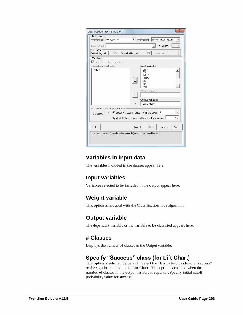
Frontline Solvers V12.5 User Guide Page 293
Variables in input data
The variables included in the dataset appear here.
Input variables
Variables selected to be included in the output appear here.
Weight variable
This option is not used with the Classification Tree algorithm.
Output variable
The dependent variable or the variable to be classified appears here.
# Classes
Displays the number of classes in the Output variable.
Specify “Success” class (for Lift Chart) This option is selected by default. Select the class to be considered a “success”
or the significant class in the Lift Chart. This option is enabled when the
number of classes in the output variable is equal to 2Specify initial cutoff
probability value for success.

Frontline Solvers V12.5 User Guide Page 294
Specify initial cutoff probability value for success
Enter a value between 0 and 1 here to denote the cutoff probability for success.
If the calculated probability for success for an observation is greater than or
equal to this value, than a “success” (or a 1) will be predicted for that
observation. If the calculated probability for success for an observation is less
than this value, then a “non-success” (or a 0) will be predicted for that
observation. The default value is 0.5. This option is only enabled when the # of
classes is equal to 2.
Normlize input data
XLMiner will normalize the data when Normalize input data is selected.
Normalization helps only if linear combinations of the input variables are used
when splitting the tree. This option is not selected by default.
Minimum #records in a terminal node
Select Minimum #records in a terminal node to stop the training data as soon as
the number of records in a node reaches the specified minimum value. By
default, the value is set to 10% of the number of training records.
Prune Tree
XLMiner will prune the tree using the validation set when Prune Tree is
selected. (Pruning the tree using the validation set will reduce the error from
over-fitting the tree using the training data.) This option is selected by default.
If no validation set exists, then this option is disabled.

Frontline Solvers V12.5 User Guide Page 295
Maximum # levels to be displayed
XLMiner provides the option to provide maximum #levels in the tree. The
default level is 5.
Full tree (grown using training data)
Select this option to “grow” a complete tree using the training data.
Best pruned tree (pruned using validation data)
Selecting this option will result in a tree with the fewest number of nodes,
subject to the constraint that the error be kept below a specified level (minimum
error rate plus the standard error of that error rate).
Minimum error tree (pruned using validation data)
Select this option to produce a tree that yields the minimum classification error
rate when tested on the validation data.
Tree with specified number of decision nodes
To create a tree with a specified number of decision nodes select this option and
enter the desired number of nodes.

Frontline Solvers V12.5 User Guide Page 296
Score training data
Select these options to show an assessment of the performance of the tree in
classifying the training data. The report is displayed according to your
specifications - Detailed, Summary and Lift charts.
Score validation data
Select these options to show an assessment of the performance of the tree in
classifying the validation data. The report is displayed according to your
specifications - Detailed, Summary and Lift charts.
Score test data
These options are enabled when a test set is present. Select these options to
show an assessment of the performance of the tree in classifying the test data.
The report is displayed according to your specifications - Detailed, Summary
and Lift charts.
Score new data
Please see the Scoring chapter for information on the Score new data options.

Frontline Solvers V12.5 User Guide Page 297
Naïve Bayes Classification Method
Introduction Suppose your data consists of fruits, described by their color and shape.
Bayesian classifiers operate by saying "If you see a fruit that is red and round,
which type of fruit is it most likely to be? In the future, classify red and round
fruit as that type of fruit."
A difficulty arises when you have more than a few variables and classes – an
enormous number of observations (records) would be required to estimate these
probabilities.
The Naive Bayes classification method avoids this problem by not requiring a
large number of observations for each possible combination of the variables.
Rather, the variables are assumed to be independent of one another and,
therefore the probability that a fruit that is red, round, firm, 3" in diameter, etc.
will be an apple can be calculated from the independent probabilities that a fruit
is red, that it is round, that it is firm, that it is 3" in diameter, etc.
In other words, Naïve Bayes classifiers assume that the effect of a variable value
on a given class is independent of the values of other variables. This assumption
is called class conditional independence and is made to simplify the
computation. In this sense, it is considered to be “Naïve”.
This assumption is a fairly strong assumption and is often not applicable.
However, bias in estimating probabilities often may not make a difference in
practice -- it is the order of the probabilities, not their exact values, which
determine the classifications.
Studies comparing classification algorithms have found the Naïve Bayesian
classifier to be comparable in performance with classification trees and neural
network classifiers. It has also been found that these classifiers exhibit high
accuracy and speed when applied to large databases.
A more technical description of the Naïve Bayesian classification method
follows.
Bayes Theorem
Let X be the data record (case) whose class label is unknown. Let H be some
hypothesis, such as "data record X belongs to a specified class C." For
classification, we want to determine P (H|X) -- the probability that the
hypothesis H holds, given the observed data record X.
P (H|X) is the posterior probability of H conditioned on X. For example, the
probability that a fruit is an apple, given the condition that it is red and round. In
contrast, P(H) is the prior probability, or apriori probability, of H. In this
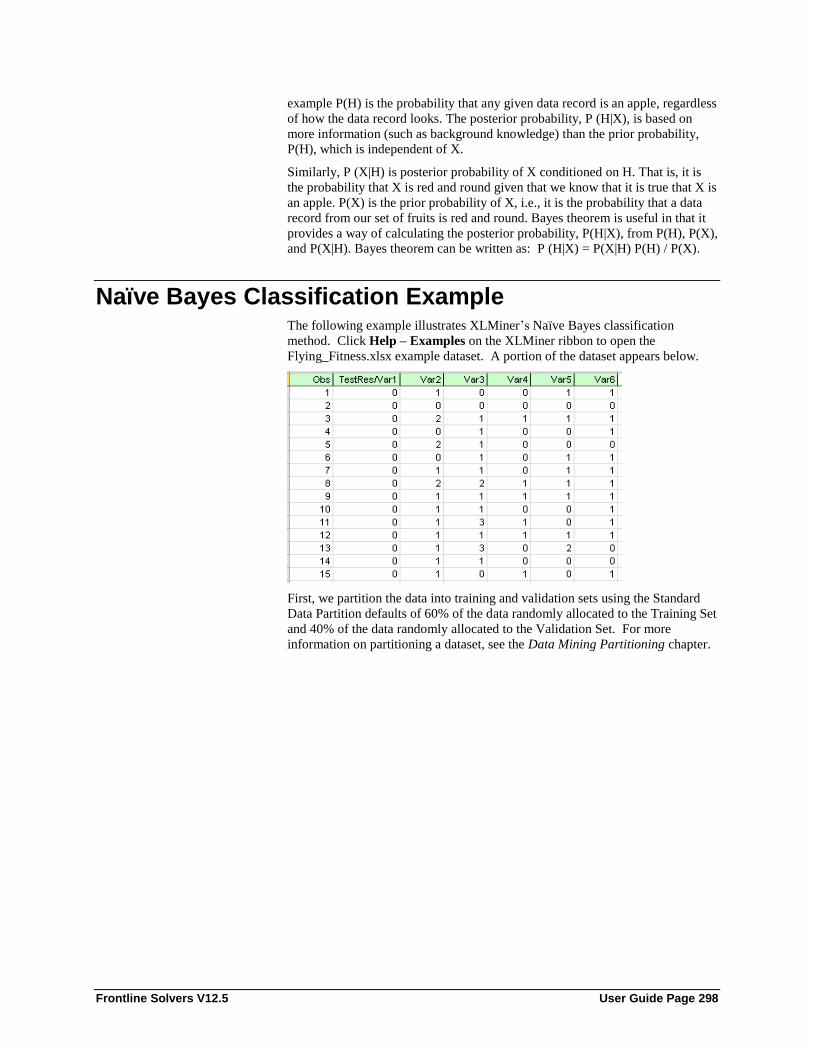
Frontline Solvers V12.5 User Guide Page 298
example P(H) is the probability that any given data record is an apple, regardless
of how the data record looks. The posterior probability, P (H|X), is based on
more information (such as background knowledge) than the prior probability,
P(H), which is independent of X.
Similarly, P (X|H) is posterior probability of X conditioned on H. That is, it is
the probability that X is red and round given that we know that it is true that X is
an apple. P(X) is the prior probability of X, i.e., it is the probability that a data
record from our set of fruits is red and round. Bayes theorem is useful in that it
provides a way of calculating the posterior probability, P(H|X), from P(H), P(X),
and P(X|H). Bayes theorem can be written as: P (H|X) = P(X|H) P(H) / P(X).
Naïve Bayes Classification Example The following example illustrates XLMiner’s Naïve Bayes classification
method. Click Help – Examples on the XLMiner ribbon to open the
Flying_Fitness.xlsx example dataset. A portion of the dataset appears below.
First, we partition the data into training and validation sets using the Standard
Data Partition defaults of 60% of the data randomly allocated to the Training Set
and 40% of the data randomly allocated to the Validation Set. For more
information on partitioning a dataset, see the Data Mining Partitioning chapter.

Frontline Solvers V12.5 User Guide Page 299
Select a cell on the Data_Partition1 worksheet, then click Classify – Naïve
Bayes. The following Naïve Bayes Step 1 of 3 dialog appears.

Frontline Solvers V12.5 User Guide Page 300
Select Var2, Var3, Var4, Var5, and Var6 as Input variables and
TestRest/Var1 as the Output variable. The # Classes statistic will be
automatically updated with a value of 2 when the Output variable is selected.
This indicates that the Output variable, TestRest/Var1 contains two classes, 0
and 1.
Choose the value that will be the indicator of “Success” by clicking the down
arrow next to Specify “Success” class (necessary). In this example, we will use
the default of 1 indicating that a value of “1” will be specified as a “success”.
Enter a value between 0 and 1 for Specify the initial cutoff probability for
success. If the Probability of success (probability of the output variable = 1) is
less than this value, then a 0 will be entered for the class value, otherwise a 1
will be entered for the class value. In this example, we will keep the default of
0.5.

Frontline Solvers V12.5 User Guide Page 301
Click Next to advance to Step 2 of 3 of the Naïve Bayes algorithm.
On the Step 2 of 3 dialog, select According to relative occurrences in training
data to calculate the Prior class probabilities. When this option is selected,
XLMiner will calculate the class probabilities from the training data . For the
first class, XLMiner will calculate the probability using the number of “0”
records / total number of points. For the second class, XLMiner will calculate
the probability using the number of “1” records / total number of points. When
Use equal prior probabilities is selected, XLMiner will use 0.5 probability in
both classes. The third option, User specified prior probabilities, is not
supported in this method.
Click Next to advance to the Step 3 of 3 dialog.

Frontline Solvers V12.5 User Guide Page 302
Select Detailed report, Summary report, and Lift charts under both Score
training data and Score validation data to obtain the complete output results for
this classification method.
For more information on the options for Score new data, please see the Scoring
chapter.
Click Finish to generate the output.
Click the NNB_Output1 worksheet to display the Output Navigator. Click any
link to navigate to the selected topic.

Frontline Solvers V12.5 User Guide Page 303
Click the NNB_ValidScore1 worksheet to view the Classification of Validation
Data table, shown below. While predicting the class of output variable,
XLMiner calculates the conditional probability that the variable may be
classified to a particular class. In this case the classes are 0 and 1. For every
record in the validation data the conditional probabilities for class - 0 and for
class - 1 are calculated as shown below. The maximum value amongst these
probabilities is highlighted. XLMiner assigns that class to the output variable,
for which the conditional probability is the largest.
Click the Prior Class Pr link on the Output Navigator to view the Prior Class
Probabilities table on the NNB_Output1 worksheet. As shown, 54.17% of the

Frontline Solvers V12.5 User Guide Page 304
training data records belonged to the “1” class and 45.83% of the training data
records belong to the “0” class.
Click the Conditional Probabilities link to display the table below. This table
shows the probabilities for each case for each variable. For example, for Var2,
15.38% of the cases were classified as “0”, 84.62% of the cases were classified
as “1” and 0 cases were classified as “2”.
Click the Training Lift Chart and Validation Lift Chart links.

Frontline Solvers V12.5 User Guide Page 305
Lift charts are visual aids for measuring model performance. They consist of a
lift curve and a baseline. The greater the area between the lift curve and the
baseline, the better the model.
After the model is built using the training data set, the model is used to score on
the training data set and the validation data set. Then the data sets are sorted
using the predicted output variable value. After sorting, the actual outcome
values of the output variable are cumulated and the lift curve is drawn as the
number of cases versus the cumulated value. The baseline is drawn as the
number of cases versus the average of actual output variable values multiplied
by the number of cases. The decilewise lift curve is drawn as the decile number
versus the cumulative actual output variable value divided by the decile's
average output variable value.
Please see the Scoring chapter for information on the worksheet NNB_Stored_1.
Naïve Bayes Classification Method Options The options below appear on one of the three Naïve Bayes classification
methods’ dialogs.
Variables in input data
The variables included in the dataset appear here.
Input variables
Variables selected to be included in the output appear here.

Frontline Solvers V12.5 User Guide Page 306
Weight variable
This option is not used with the Naïve Bayes algorithm.
Output variable
The dependent variable or the variable to be classified appears here.
# Classes
Displays the number of classes in the Output variable.
Specify “Success” class (for Lift Chart) This option is selected by default. Select the class to be considered a “success”
or the significant class in the Lift Chart. This option is enabled when the
number of classes in the output variable is equal to 2Specify initial cutoff
probability value for success.
Specify initial cutoff probability value for success
Enter a value between 0 and 1 here to denote the cutoff probability for success.
If the calculated probability for success for an observation is greater than or
equal to this value, than a “success” (or a 1) will be predicted for that
observation. If the calculated probability for success for an observation is less
than this value, then a “non-success” (or a 0) will be predicted for that
observation. The default value is 0.5. This option is only enabled when the # of
classes is equal to 2.
According to relative occurrences in training data When this option is selected, XLMiner will calculate the class probabilities from
the training data . For the first class, XLMiner will calculate the probability
using the number of “0” records / total number of points. For the second class,
XLMiner will calculate the probability using the number of “1” records / total
number of points.

Frontline Solvers V12.5 User Guide Page 307
Use equal prior probabilities
When this option is selected, XLMiner will use 0.5 probability for both classes.
User specified prior probabilities
This option is not supported in this method.
Score training data
Select these options to show an assessment of the performance of the tree in
classifying the training data. The report is displayed according to your
specifications - Detailed, Summary and Lift charts.
Score validation data
Select these options to show an assessment of the performance of the tree in
classifying the validation data. The report is displayed according to your
specifications - Detailed, Summary and Lift charts.
Score test data
These options are enabled when a test set is present. Select these options to
show an assessment of the performance of the tree in classifying the test data.
The report is displayed according to your specifications - Detailed, Summary
and Lift charts.
Score new data
Please see the Scoring chapter for information on the Score new data options.
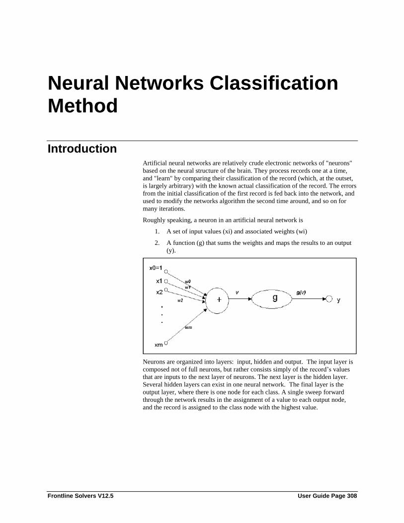
Frontline Solvers V12.5 User Guide Page 308
Neural Networks Classification Method
Introduction Artificial neural networks are relatively crude electronic networks of "neurons"
based on the neural structure of the brain. They process records one at a time,
and "learn" by comparing their classification of the record (which, at the outset,
is largely arbitrary) with the known actual classification of the record. The errors
from the initial classification of the first record is fed back into the network, and
used to modify the networks algorithm the second time around, and so on for
many iterations.
Roughly speaking, a neuron in an artificial neural network is
1. A set of input values (xi) and associated weights (wi)
2. A function (g) that sums the weights and maps the results to an output
(y).
Neurons are organized into layers: input, hidden and output. The input layer is
composed not of full neurons, but rather consists simply of the record’s values
that are inputs to the next layer of neurons. The next layer is the hidden layer.
Several hidden layers can exist in one neural network. The final layer is the
output layer, where there is one node for each class. A single sweep forward
through the network results in the assignment of a value to each output node,
and the record is assigned to the class node with the highest value.

Frontline Solvers V12.5 User Guide Page 309
Training an Artificial Neural Network
In the training phase, the correct class for each record is known (this is termed
supervised training), and the output nodes can therefore be assigned "correct"
values -- "1" for the node corresponding to the correct class, and "0" for the
others. (In practice, better results have been found using values of “0.9” and
“0.1”, respectively.) It is thus possible to compare the network's calculated
values for the output nodes to these "correct" values, and calculate an error term
for each node (the "Delta" rule). These error terms are then used to adjust the
weights in the hidden layers so that, hopefully, during the next iteration the
output values will be closer to the "correct" values.
The Iterative Learning Process
A key feature of neural networks is an iterative learning process in which
records (rows) are presented to the network one at a time, and the weights
associated with the input values are adjusted each time. After all cases are
presented, the process is often repeated. During this learning phase, the network
“trains” by adjusting the weights to predict the correct class label of input
samples. Advantages of neural networks include their high tolerance to noisy
data, as well as their ability to classify patterns on which they have not been
trained. The most popular neural network algorithm is the back-propagation
algorithm proposed in the 1980's.
Once a network has been structured for a particular application, that network is
ready to be trained. To start this process, the initial weights (described in the
next section) are chosen randomly. Then the training, or learning, begins.
The network processes the records in the training data one at a time, using the
weights and functions in the hidden layers, then compares the resulting outputs
against the desired outputs. Errors are then propagated back through the system,
causing the system to adjust the weights for application to the next record. This
process occurs over and over as the weights are continually tweaked. During the
training of a network the same set of data is processed many times as the
connection weights are continually refined.
Note that some networks never learn. This could be because the input data does
not contain the specific information from which the desired output is derived.
Networks also will not converge if there is not enough data to enable complete
learning. Ideally, there should be enough data available to create a validation set.

Frontline Solvers V12.5 User Guide Page 310
Feedforward, Back-Propagation
The feedforward, back-propagation architecture was developed in the early
1970's by several independent sources (Werbor; Parker; Rumelhart, Hinton and
Williams). This independent co-development was the result of a proliferation of
articles and talks at various conferences which stimulated the entire industry.
Currently, this synergistically developed back-propagation architecture is the
most popular, effective, and easy-to-learn model for complex, multi-layered
networks. Its greatest strength is in non-linear solutions to ill-defined problems.
The typical back-propagation network has an input layer, an output layer, and at
least one hidden layer. There is no theoretical limit on the number of hidden
layers but typically there are just one or two. Some studies have shown that the
total number of layers needed to solve problems of any complexity is 5 (one
input layer, three hidden layers and an output layer). Each layer is fully
connected to the succeeding layer.
As noted above, the training process normally uses some variant of the Delta
Rule, which starts with the calculated difference between the actual outputs and
the desired outputs. Using this error, connection weights are increased in
proportion to the error times, which are a scaling factor for global accuracy. This
means that the inputs, the output, and the desired output all must be present at
the same processing element. The most complex part of this algorithm is
determining which input contributed the most to an incorrect output and how
must the input be modified to correct the error. (An inactive node would not
contribute to the error and would have no need to change its weights.) To solve
this problem, training inputs are applied to the input layer of the network, and
desired outputs are compared at the output layer. During the learning process, a
forward sweep is made through the network, and the output of each element is
computed layer by layer. The difference between the output of the final layer
and the desired output is back-propagated to the previous layer(s), usually
modified by the derivative of the transfer function. The connection weights are
normally adjusted using the Delta Rule. This process proceeds for the previous
layer(s) until the input layer is reached.
Structuring the Network
The number of layers and the number of processing elements per layer are
important decisions. These parameters, to a feedforward, back-propagation
topology, are also the most ethereal - they are the "art" of the network designer.
There is no quantifiable, best answer to the layout of the network for any
particular application. There are only general rules picked up over time and
followed by most researchers and engineers applying this architecture to their
problems.
Rule One: As the complexity in the relationship between the input data and the
desired output increases, the number of the processing elements in the hidden
layer should also increase.
Rule Two: If the process being modeled is separable into multiple stages, then
additional hidden layer(s) may be required. If the process is not separable into
stages, then additional layers may simply enable memorization of the training
set, and not a true general solution.
Rule Three: The amount of training data available sets an upper bound for the
number of processing elements in the hidden layer(s). To calculate this upper
bound, use the number of cases in the training data set and divide that number
by the sum of the number of nodes in the input and output layers in the network.

Frontline Solvers V12.5 User Guide Page 311
Then divide that result again by a scaling factor between five and ten. Larger
scaling factors are used for relatively less noisy data. If too many artificial
neurons are used the training set will be memorized, not generalized, and the
network will be useless on new data sets.
Automated Neural Network Classification Example The example below illustrates the use of XLMiner’s Automated Neural
Networks Classification method. Click Help – Examples on the XLMiner
ribbon to open the file Wine.xlsx. This file contains 13 quantitative variables
measuring the chemical attributes of wine samples from 3 different wineries
(Type variable). The objective is to assign a wine classification to each record.
A portion of this dataset is shown below.
First, we partition the data into training and validation sets using a Standard
Data Partition with percentages of 80% of the data randomly allocated to the
Training Set and 20% of the data randomly allocated to the Validation Set. For
more information on partitioning a dataset, see the Data Mining Partitioning
chapter.

Frontline Solvers V12.5 User Guide Page 312
Select a cell on the newly created Data_Partition1 worksheet, then click
Classify – Neural Network on the XLMiner ribbon. The following dialog
appears.

Frontline Solvers V12.5 User Guide Page 313
Select Type as the Output variable and the remaining variables as Input
Variables. Since the Output variable contains three classes (A, B, and C) to
denote the three different wineries, the options for Classes in the output variable
are disabled.
XLMiner also allows a “Weight variable”. This option can be used if the data
contains multiple cases (objects) sharing the same variable values. The weight
variable denotes the number of cases with those values.

Frontline Solvers V12.5 User Guide Page 314
Click Next to advance to the next dialog.
This dialog contains the options to define the network architecture. Select
Normalize input data. Normalizing the data (subtracting the mean and
dividing by the standard deviation) is important to ensure that the distance
measure accords equal weight to each variable -- without normalization, the
variable with the largest scale would dominate the measure.

Frontline Solvers V12.5 User Guide Page 315
XLMiner provides two options for the Network Architecture -- Automatic and
Manual. The default network architecture is 'Automatic'. This option generates
several neural networks in the output sheet for various combinations of hidden
layers and nodes within each layer. The total number of the neural networks
generated using the 'Automatic' option currently is 100. Choose the Manual
option to specify the number of hidden layers and the number of nodes for one
neural network. Please see the example below for explanations of the various
fields to be specified when the "Manual' network architecture is chosen is as
follows. For this example, keep the default setting of Automatic. See the next
example for an illustration of how to use the Manual Network Architecture
setting.
Keep the default setting of 30 for # Epochs. An epoch is one sweep through all
records in the training set.
Keep the default setting of 0.1 for Step size for gradient descent. This is the
multiplying factor for the error correction during backpropagation; it is roughly
equivalent to the learning rate for the neural network. A low value produces
slow but steady learning, a high value produces rapid but erratic learning.
Values for the step size typically range from 0.1 to 0.9.
Keep the default setting of 0.6 for Weight change momentum. In each new
round of error correction, some memory of the prior correction is retained so
that an outlier that crops up does not spoil accumulated learning.
Keep the default setting of 0.01 for Error tolerance. The error in a particular
iteration is backpropagated only if it is greater than the error tolerance. Typically
error tolerance is a small value in the range from 0 to 1.
Keep the default setting of 0 for Weight decay. To prevent over-fitting of the
network on the training data, set a weight decay to penalize the weight in each
iteration. Each calculated weight will be multiplied by (1-decay).
XLMiner provides four options for cost functions -- Squared mirror, Cross
entropy, Maximum likelihood and Perceptron convergence. The user can select
the appropriate one. Keep the default selection, Squared error, for this example.
Nodes in the hidden layer receive input from the input layer. The output of the
hidden nodes is a weighted sum of the input values. This weighted sum is
computed with weights that are initially set at random values. As the network
“learns” these weights are adjusted. This weighted sum is used to compute the
hidden node’s output using a transfer function. Select Standard (the default
setting) to use a logistic function for the transfer function with a range of 0 and
1. This function has a “squashing effect” on very small or very large values but
is almost linear in the range where the value of the function is between 0.1 and
0.9.3 Select Symmetric to use the tanh function for the transfer function, the
range being -1 to 1. Keep the default selection, Standard, for this example. If
more than one hidden layer exists, this function is used for all layers.
As in the hidden layer output calculation (explained in the above paragraph), the
output layer is also computed using the same transfer function. Select Standard
(the default setting) to use a logistic function for the transfer function with a
range of 0 and 1. Select Symmetric to use the tanh function for the transfer
function, the range being -1 to 1. Keep the default selection, Standard, for this
example.
3Galit Shmueli, Nitin R. Patel, and Peter C. Bruce, Data Mining for Business Intelligence (New Jersey: Wiley, 2010) 226.

Frontline Solvers V12.5 User Guide Page 316
Since Automatic is selected for Network Architecture, the Next button is
disabled. Click Finish. The Automatic_NNC1 worksheet containing the output
will be inserted at the end of the workbook.
The top section of this worksheet includes the Output Navigator which can be
used to quickly navigate to various sections of the output. The Data, Variables,
and Parameters/Options sections of the output worksheet all reflect inputs
chosen by the user.
A little further down is the Error Report, a portion is shown below.

Frontline Solvers V12.5 User Guide Page 317
The above error report gives the total number of errors and the % error in
classification produced by each network ID for the training and validation sets
separately. For example: Net 26 has 2 hidden layers each having one node in
each hidden layer. For this neural network, the percentage of errors in the
training data is 72.54% and the percentage of errors in the validation data is
75%.
XLMiner provides sorting of the error report according to increasing or
decreasing order of the %Error by clicking the up arrow next to % Error. Click
the upgrade arrow to sort in ascending order, and the downward arrow to sort in
descending order.
If you click a hyperlink for a particular Net ID (say Net 26) in the Error Report,
the following dialog appears. Here, the user can select the various options for
scoring data on Net ID 26. See the example below for more on this dialog and
the associated output.
Click Cancel to return to the Automated_NNCOutput1 worksheet. Scroll down
to the final section of this worksheet to find the Confusion matrices for all Net
IDs in the training and validation datasets.

Frontline Solvers V12.5 User Guide Page 318
Manual Neural Network Classification Example Refer to the example above to advance to the Neural Network (MultiLayer
Feedforward) Step 2 of 3 dialog, shown below.
This example will use the same dataset to illustrate the use of the Manual
Network Architecture selection.
Follow the steps above for the Step 1 of 3 dialog. On the Step 2 of 3 dialog,
keep the default setting of 1 for the # hidden layers option. Up to four hidden
layers can be specified for this option.
Keep the default setting of 25 for #Nodes. (Since # hidden layers is set to 1,
only the first text box is enabled.)

Frontline Solvers V12.5 User Guide Page 319
Keep the default settings for the remaining options.
Click Next to advance to the Step 3 of 3 dialog.
Select Detailed report and Summary report under both Score training data
and Score validation data.
For more information on the Score new data options, see the Scoring chapter.

Frontline Solvers V12.5 User Guide Page 320
Click Finish to produce the output.
Click the NNC_Output1 worksheet to view the Output Navigator.
Click the Training Epoch Log to display the Neural Network Classification Log.
XLMiner also provides intermediate information produced during the last pass
through the network
Scroll down on the Output1 worksheet to the Interlayer connections' weights
table.

Frontline Solvers V12.5 User Guide Page 321
Recall that a key element in a neural network is the weights for the connections
between nodes. In this example, we chose to have one hidden layer, and we also
chose to have 25 nodes in that layer. XLMiner's output contains a section that
contains the final values for the weights between the input layer and the hidden
layer, between hidden layers, and between the last hidden layer and the output
layer. This information is useful at viewing the “insides” of the neural network;
however, it is unlikely to be of use to the data analyst end-user. Displayed above
are the final connection weights between the input layer and the hidden layer for
our example.
Click the Training Epoch Log link on the Output Navigator to display the
following log.

Frontline Solvers V12.5 User Guide Page 322
During an epoch, each training record is fed forward in the network and
classified. The error is calculated and is back propagated for the weights
correction. Weights are continuously adjusted during the epoch. The
classification error is computed as the records pass through the network. It does
not report the classification error after the final weight adjustment. Scoring of
the training data is performed using the final weights so the training
classification error may not exactly match with the last epoch error in the Epoch
log.
See the Scoring chapter for information on Stored Model Sheets,
NNC_Stored_1.
NNC with Output Variable Containing 2 Classes The Error Report for a dataset with 2 classes in the output variable will look
slightly different. Open the file Boston_Housing.xlsx by clicking Help –
Examples on the XLMiner ribbon. Partition the data as shown in the two
previous Neural Network examples.
Select a cell on the Data_Partition1 worksheet, then click Classify – Neural
Network on the XLMiner ribbon. Select CAT.MEDV (has 2 classes) for the
Output variable and the remaining variables (except MEDV) as Input variables.
Click Next to proceed to the Step 2 of 3 dialog.

Frontline Solvers V12.5 User Guide Page 323
The Step 2 of 3 dialog contains options to define the network architecture. For
this example, accept the default values. (Details on these choices are explained
in the above examples.)
Click Finish to produce the Automated_NNC1 output worksheet. Scroll down
to the Error Report.

Frontline Solvers V12.5 User Guide Page 324
The above error report gives the total number of errors, % Error, % Sensitivity
and % Specificity in the classification produced by each network ID for the
training and validation datasets separately. For example: Net 10 has one hidden
layer having 10 nodes. For this neural network, the percentage of errors in the
training data is 4.69% and the percentage of errors in the validation data is
3.96%. The percentage sensitivity is 76.92% and 84.21% for training data and
validation data respectively. The percentage specificity is 98.82% and 98.78%
for training data and validation data respectively.
Numerically, sensitivity is the number of true positive results (TP) divided by
the sum of true positive and false negative (FN) results,
i.e., sensitivity = TP/(TP + FN).
Numerically, specificity is the number of true negative results (TN) divided by
the sum of true negative and false positive (FP) results,
i.e., specificity = TN/(TN + FP).
XLMiner provides sorting of the error report according to increasing or
decreasing order of the %Error, %Sensitivity or %Specificity. This can be done
by clicking the up arrow next to %Error, %Sensitivity or %Specificity,
respectively. Click the upward arrow to sort in ascending order, and the
downward arrow to sort in descending order.
Neural Network Classification Method Options The options below appear on one of the three Neural Network Classification
dialogs.

Frontline Solvers V12.5 User Guide Page 325
Variables in input data
The variables included in the dataset appear here.
Input variables
Variables selected to be included in the output appear here.
Weight variable
This option is not used with the Neural Network Classification algorithm.
Output variable
The dependent variable or the variable to be classified appears here.
# Classes
Displays the number of classes in the Output variable.
Specify “Success” class (for Lift Chart)
This option is selected by default. Click the drop down arrow to select the value
to specify a “success”. This option is only enabled when the # of classes is
equal to 2.

Frontline Solvers V12.5 User Guide Page 326
Specify initial cutoff probability value for success
Enter a value between 0 and 1 here to denote the cutoff probability for success.
If the calculated probability for success for an observation is greater than or
equal to this value, than a “success” (or a 1) will be predicted for that
observation. If the calculated probability for success for an observation is less
than this value, then a “non-success” (or a 0) will be predicted for that
observation. The default value is 0.5. This option is only enabled when the # of
classes is equal to 2.
Normalize input data
Normalizing the data (subtracting the mean and dividing by the standard
deviation) is important to ensure that the distance measure accords equal weight
to each variable -- without normalization, the variable with the largest scale
would dominate the measure. This option is selected by default.
Network Architecture
XLMiner provides two options for the Network Architecture -- Automatic and
Manual. The default network architecture is 'Automatic'. This option generates
several neural networks in the output sheet for various combinations of hidden
layers and nodes within each layer. The total number of the neural networks
generated using the 'Automatic' option currently is 100. Choose the Manual
option to specify the number of hidden layers and the number of nodes for one
neural network.
# Hidden Layers
When Manual is selected, this option is enabled. XLMiner supports up to 4
hidden layers.

Frontline Solvers V12.5 User Guide Page 327
# Nodes
When Manual is selected, this option is enabled. Enter the number of nodes per
layer here.
# Epochs
An epoch is one sweep through all records in the training set. The default
setting is 30.
Step size for gradient descent
This is the multiplying factor for the error correction during backpropagation; it
is roughly equivalent to the learning rate for the neural network. A low value
produces slow but steady learning, a high value produces rapid but erratic
learning. Values for the step size typically range from 0.1 to 0.9. The default
setting is 0.1.
Weight change momentum
In each new round of error correction, some memory of the prior correction is
retained so that an outlier that crops up does not spoil accumulated learning.
The default setting is 0.6.
Error tolerance
The error in a particular iteration is backpropagated only if it is greater than the
error tolerance. Typically error tolerance is a small value in the range from 0 to
1. The default setting is 0.01.
Weight decay
To prevent over-fitting of the network on the training data, set a weight decay to
penalize the weight in each iteration. Each calculated weight will be multiplied
by (1-decay). The default setting is 0.
Cost Function
XLMiner provides four options for the cost function -- Squared mirror, Cross
entropy, Maximum likelihood and Perceptron convergence. The user can select
the appropriate one. The default setting is Squared error.
Hidden Layer Sigmoid
Nodes in the hidden layer receive input from the input layer. The output of the
hidden nodes is a weighted sum of the input values. This weighted sum is
computed with weights that are initially set at random values. As the network
“learns”, these weights are adjusted. This weighted sum is used to compute the
hidden node’s output using a transfer function. Select Standard (the default
setting) to use a logistic function for the transfer function with a range of 0 and
1. This function has a “squashing effect” on very small or very large values but
is almost linear in the range where the value of the function is between 0.1 and
0.9. Select Symmetric to use the tanh function for the transfer function, the

Frontline Solvers V12.5 User Guide Page 328
range being -1 to 1. If more than one hidden layer exists, this function is used
for all layers. The default selection is Standard.
Output Layer Sigmoid
As in the hidden layer output calculation (explained in the above paragraph), the
output layer is also computed using the same transfer function as described for
Hidden Layer Sigmoid. Select Standard (the default setting) to use a logistic
function for the transfer function with a range of 0 and 1. Select Symmetric to
use the tanh function for the transfer function, the range being -1 to 1. The
default selection is Standard.
Score training data
Select these options to show an assessment of the performance of the tree in
classifying the training data. The report is displayed according to your
specifications - Detailed, Summary and Lift charts.
Score validation data
Select these options to show an assessment of the performance of the tree in
classifying the validation data. The report is displayed according to your
specifications - Detailed, Summary and Lift charts.
Score test data
These options are enabled when a test set is present. Select these options to
show an assessment of the performance of the tree in classifying the test data.
The report is displayed according to your specifications - Detailed, Summary
and Lift charts.

Frontline Solvers V12.5 User Guide Page 329
Score New Data See the Scoring chapter for more details on the In worksheet or In database
options.

Frontline Solvers V12.5 User Guide Page 330
Multiple Linear Regression Prediction Method
Introduction Linear regression is performed on a dataset either to predict the response
variable based on the predictor variable, or to study the relationship between the
response variable and predictor variables. For example, using linear regression,
the crime rate of a state can be explained as a function of demographic factors
such as population, education, male to female ratio etc.
This procedure performs linear regression on a selected dataset that fits a linear
model of the form
Y= b0 + b1X1 + b2X2+ .... + bkXk+ e
where Y is the dependent variable (response), X1, X2,.. .,Xk are the independent
variables (predictors) and e is the random error. b0 , b1, b2, .... bk are known as
the regression coefficients, which are estimated from the data. The multiple
linear regression algorithm in XLMiner chooses regression coefficients to
minimize the difference between the predicted and actual values.
Multiple Linear Regression Example The following example illustrates XLMiner’s Multiple Linear Regression
method using the Boston Housing dataset to predict the median house price in
housing tracts in the Boston area. This dataset has 14 variables. A description of
each variable is given in the table below. In addition to these variables, the data
set also contains an additional variable, which has been created by categorizing
median value (MEDV) into two categories – high (MEDV > 30) and low
(MEDV < 30).
CRIM Per capita crime rate by town ZN Proportion of residential land zoned for lots over 25,000 sq.ft. INDUS Proportion of non-retail business acres per town CHAS Charles River dummy variable (= 1 if tract bounds river; 0 otherwise) NOX Nitric oxides concentration (parts per 10 million) RM Average number of rooms per dwelling AGE Proportion of owner-occupied units built prior to 1940 DIS Weighted distances to five Boston employment centers RAD Index of accessibility to radial highways TAX Full-value property-tax rate per $10,000 PTRATIO Pupil-teacher ratio by town B 1000(Bk - 0.63)^2 where Bk is the proportion of African-Americans
by town LSTAT % Lower status of the population MEDV Median value of owner-occupied homes in $1000's

Frontline Solvers V12.5 User Guide Page 331
Click Help – Examples on the XLMiner ribbon to open the
Boston_Housing.xlsx from the datasets folder. A portion of the dataset is shown
below.
First, we partition the data into training and validation sets using the Standard
Data Partition defaults with percentages of 60% of the data randomly allocated
to the Training Set and 40% of the data randomly allocated to the Validation
Set. For more information on partitioning a dataset, see the Data Mining
Partitioning chapter.
Select a cell on the Data_Partition1 worksheet, then click Predict – Multiple
Linear Regression. The following dialog appears.

Frontline Solvers V12.5 User Guide Page 332
Select MEDV as the Output variable and all remaining variables (except CAT.
MEDV) as Input variables. (The bottom portion of the dialog is not used with
prediction methods.)

Frontline Solvers V12.5 User Guide Page 333
Click Next to advance to the Step 2 of 2 dialog.
If the number of rows in the data is less than the number of variables selected as
Input variables, XLMiner displays the following message box.
Select Yes to proceed to the Best Subset dialog (see below). Click No to return
to the Multiple Linear Regression Step 1 of 2 dialog.
If Force constant term to zero is selected, there will be no constant term in the
equation. Leave this option unchecked for this example.
Select Fitted values. When this option is selected, the fitted values are
displayed in the output.
Select ANOVA table. When this option is selected, the ANOVA table is
displayed in the output.
Select Standardized under Residuals to display the Standardized Residuals in
the output. Standardized residuals are obtained by dividing the unstandardized
residuals by the respective standard deviations.

Frontline Solvers V12.5 User Guide Page 334
Select Unstandardized under Residuals to display the Unstandardized
Residuals in the output. Unstandardized residuals are computed by the formula:
Unstandardized residual = Actual response – Predicted response.
Select Variance-covariance matrix. When this option is selected the variance-
covariance matrix of the estimated regression coefficients is displayed in the
output.
Select all options under Score Training data and Score validation data to
produce all three reports in the output.
Click Advanced to display the following dialog.

Frontline Solvers V12.5 User Guide Page 335
Select Studentized. When this option is selected the Studentized Residuals are
displayed in the output. Studentized residuals are computed by dividing the
unstandardized residuals by quantities related to the diagonal elements of the hat
matrix, using a common scale estimate computed without the ith
case in the
model. These residuals have t - distributions with ( n-k-1) degrees of freedom.
As a result, any residual with absolute value exceeding 3 usually requires
attention.
Select Deleted. When this option is selected the Deleted Residuals are
displayed in the output. This residual is computed for the ith
observation by first
fitting a model without the ith
observation, then using this model to predict the ith
observation. Afterwards the difference is taken between the predicted
observation and the actual observation.
Select Cook's Distance. When this checkbox is selected the Cook's Distance
for each observation is displayed in the output. This is an overall measure of the
impact of the ith
datapoint on the estimated regression coefficient. In linear
models Cook's Distance has, approximately, an F distribution with k and (n-k)
degrees of freedom.
Select DF fits. When this checkbox is selected the DF fits (change in the
regression fit) for each observation is displayed in the output. These reflect
coefficient changes as well as forecasting effects when an observation is deleted.
Select Covariance Ratios. When this checkbox is selected, the covariance
ratios are displayed in the output. This measure reflects the change in the
variance-covariance matrix of the estimated coefficients when the ith
observation
is deleted.
Select Hat matrix Diagonal. When this checkbox is selected, the diagonal
elements of the hat matrix are displayed in the output. This measure is also
known as the leverage of the ith
observation.
Select Perform Collinearity diagnostics. When this checkbox is selected, the
collinearity diagnostics are displayed in the output.

Frontline Solvers V12.5 User Guide Page 336
When Perform Collinearity diagnostics is selected, Number of collinearity
components is enabled. Enter 2 for this option. This number can be between 2
and the number of degrees of freedom for the model. When the model is fitted
without an intercept, the model degrees of freedom is equal to the number of
predictors in the model. When the model is fitted with an intercept, the model
degrees of freedom is equal to the number of predictors in the model plus one.
When Perform Collinearity diagnostics is selected, Multicollinearity criterion is
enabled. Enter 0.05 for Multicollinearity criterion. Multicollinearity can be
defined as the occurrence of two or more input variables that share the same
linear relationship with the outcome variable. Enter a value between 0 and 1.
The default setting is 0.05.
Click OK to return to the Step 2 of 2 dialog, then click Best subset (on the Step
2 of 2 dialog) to open the following dialog.
When you have a large number of predictors and would like to limit the model
to only the significant variables, select Perform best subset selection to select
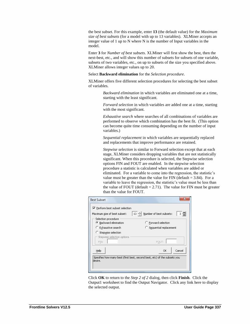
Frontline Solvers V12.5 User Guide Page 337
the best subset. For this example, enter 13 (the default value) for the Maximum
size of best subsets (for a model with up to 13 variables). XLMiner accepts an
integer value of 1 up to N where N is the number of Input variables in the
model.
Enter 3 for Number of best subsets. XLMiner will first show the best, then the
next-best, etc., and will show this number of subsets for subsets of one variable,
subsets of two variables, etc., on up to subsets of the size you specified above.
XLMiner allows integer values up to 20.
Select Backward elimination for the Selection procedure.
XLMiner offers five different selection procedures for selecting the best subset
of variables.
Backward elimination in which variables are eliminated one at a time,
starting with the least significant.
Forward selection in which variables are added one at a time, starting
with the most significant.
Exhaustive search where searches of all combinations of variables are
performed to observe which combination has the best fit. (This option
can become quite time consuming depending on the number of input
variables.)
Sequential replacement in which variables are sequentially replaced
and replacements that improve performance are retained.
Stepwise selection is similar to Forward selection except that at each
stage, XLMiner considers dropping variables that are not statistically
significant. When this procedure is selected, the Stepwise selection
options FIN and FOUT are enabled. In the stepwise selection
procedure a statistic is calculated when variables are added or
eliminated. For a variable to come into the regression, the statistic’s
value must be greater than the value for FIN (default = 3.84). For a
variable to leave the regression, the statistic’s value must be less than
the value of FOUT (default = 2.71). The value for FIN must be greater
than the value for FOUT.
Click OK to return to the Step 2 of 2 dialog, then click Finish. Click the
Output1 worksheet to find the Output Navigator. Click any link here to display
the selected output.

Frontline Solvers V12.5 User Guide Page 338
Click the Train. Score – Detailed Rep. link to open the Multiple Linear
Regression – Prediction of Training Data table. Of primary interest in a data-
mining context will be the predicted and actual values for each record, along
with the residual (difference), shown here for the training data set:
XLMiner also displays The Total sum of squared errors summaries for both the
training and validation data sets on the Output1 worksheet. The total sum of
squared errors is the sum of the squared errors (deviations between predicted
and actual values) and the root mean square error (square root of the average
squared error). The average error is typically very small, because positive
prediction errors tend to be counterbalanced by negative ones.

Frontline Solvers V12.5 User Guide Page 339
A variety of residual and collinearity diagnostics output is available since the
option was selected on the Advanced dialog (see above).
Select the Subset Selection link on the Output Navigator to display the Best
Subset Selection chart which displays a list of different models generated using
the Best Subset selections. Since we have selected 13 as the maximum size of
subsets, 13 Best Subset models have been created containing 1 to 13 variables.
A portion of this chart is shown below.
Every model includes a constant term (since Force constant term to zero was
not selected on the Step 2 of 2 dialog) and one or more variables as the
additional coefficients. We can use any of these models for further analysis by
clicking on the respective link, "Choose Subset". The choice of model depends
on the calculated values of various error values and the probability. The error
values calculated are
RSS: The residual sum of squares, or the sum of squared deviations
between the predicted probability of success and the actual value (1 or
0)
Cp: Mallows Cp (Total squared error) is a measure of the error in the
best subset model, relative to the error incorporating all variables.
Adequate models are those for which Cp is roughly equal to the
number of parameters in the model (including the constant), and/or Cp
is at a minimum
R-Squared: R-squared Goodness-of-fit
Adj. R-Squared: Adjusted R-Squared values.

Frontline Solvers V12.5 User Guide Page 340
"Probability" is a quasi hypothesis test of the proposition that a given
subset is acceptable; if Probability < .05 we can rule out that subset.
When hovering over Choose Subset, the mouse icon will change to a “grabber
hand”. If Choose Subset is clicked, XLMiner opens the Multiple Linear
Regression Step 1 of 1 dialog displaying the input variables included in that
particular subset. Scroll down to the end of the table.
Compare the RSS value as the number of coefficients in the subset increases
from 11 to 12 (8923.724 down to 6978.134). The RSS for 12 coefficients is just
slightly higher than the RSS for 14 coefficients suggesting that a model with 12
coefficients may be sufficient to fit a regression. Click the Choose Subset link
next to the first model with 12 coefficients (RSS = 6978.134), the Multiple
Linear Regression The Step 1 of 2 dialog appears with these 12 variables
already selected as Input variables. The User can easily click Next to run a
Multiple Linear Regression on these variables.
Model terms are shown in the Regression Model output shown below along
with the Summary statistics
The Regression Model table contains the coefficient, the standard error of the
coefficient, the p-value and the Sum of Squared Error for each variable included
in the model. The Sum of Squared Errors is calculated as each variable is
introduced in the model beginning with the constant term and continuing with
each variable as it appears in the dataset.
Summary statistics (to the above right) show the residual degrees of freedom
(#observations - #predictors), the R-squared value, a standard deviation type
measure for the model (which typically has a chi-square distribution), and the
Residual Sum of Squares error.
The R-squared value shown here is the r-squared value for a logistic regression
model , defined as -
R2 = (D0-D)/D0 ,

Frontline Solvers V12.5 User Guide Page 341
where D is the Deviance based on the fitted model and D0 is the deviance based
on the null model. The null model is defined as the model containing no
predictor variables apart from the constant.
Click the Collinearity Diagnostics link to display the Collinearity Diagnostics
table. This table helps assess whether two or more variables so closely track one
another as to provide essentially the same information. As you can see the NOX
variable was ignored.
The columns represent the variance components (related to principal
components in multivariate analysis), while the rows represent the variance
proportion decomposition explained by each variable in the model. The
eigenvalues are those associated with the singular value decomposition of the
variance-covariance matrix of the coefficients, while the condition numbers are
the ratios of the square root of the largest eigenvalue to all the rest. In general,
multicollinearity is likely to be a problem with a high condition number (more
than 20 or 30), and high variance decomposition proportions (say more than 0.5)
for two or more variables.
Lift charts (on the MLR_TrainLiftChart and MLR_ValidLiftChart, respectively)
are visual aids for measuring model performance. They consist of a lift curve
and a baseline. The greater the area between the lift curve and the baseline, the
better the model.
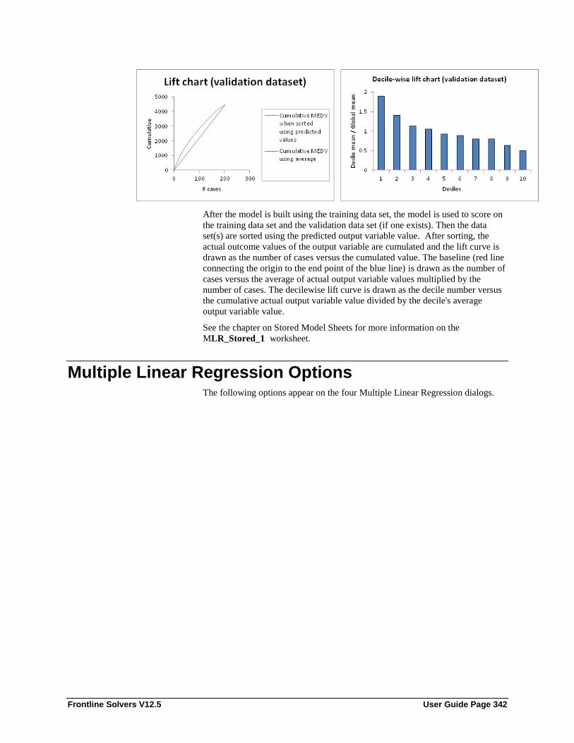
Frontline Solvers V12.5 User Guide Page 342
After the model is built using the training data set, the model is used to score on
the training data set and the validation data set (if one exists). Then the data
set(s) are sorted using the predicted output variable value. After sorting, the
actual outcome values of the output variable are cumulated and the lift curve is
drawn as the number of cases versus the cumulated value. The baseline (red line
connecting the origin to the end point of the blue line) is drawn as the number of
cases versus the average of actual output variable values multiplied by the
number of cases. The decilewise lift curve is drawn as the decile number versus
the cumulative actual output variable value divided by the decile's average
output variable value.
See the chapter on Stored Model Sheets for more information on the
MLR_Stored_1 worksheet.
Multiple Linear Regression Options The following options appear on the four Multiple Linear Regression dialogs.

Frontline Solvers V12.5 User Guide Page 343
Variables in input data
All variables in the dataset are listed here.
Input variables
Variables listed here will be utilized in the XLMiner output.
Weight variable
One major assumption of Multiple Linear Regression is that each observation
provides equal information. XLMiner offers an opportunity to provide a Weight
variable. Using a Weight variable allows the user to allocate a weight to each
record. A record with a large weight will influence the model more than a
record with a smaller weight.
Output Variable
Select the variable whose outcome is to be predicted here.

Frontline Solvers V12.5 User Guide Page 344
Force constant to zero
If this option is selected, there will be no constant term in the equation. This
option is not selected by default.
Fitted values
When this option is selected, the fitted values are displayed in the output. This
option is not selected by default.
Anova table
When this option is selected, the ANOVA table is displayed in the output. This
option is not selected by default.
Standardized
Select this option under Residuals to display the Standardized Residuals in the
output. Standardized residuals are obtained by dividing the unstandardized
residuals by the respective standard deviations. This option is not selected by
default.

Frontline Solvers V12.5 User Guide Page 345
Unstandardized
Select this option under Residuals to display the Unstandardized Residuals in
the output. Unstandardized residuals are computed by the formula:
Unstandardized residual = Actual response – Predicted response. This option is
not selected by default.
Variance – covariance matrix
When this option is selected the variance-covariance matrix of the estimated
regression coefficients is displayed in the output. This option is not selected by
default.
Score training data
Select these options to show an assessment of the performance of the tree in
classifying the training data. The report is displayed according to your
specifications - Detailed, Summary and Lift charts.
Score validation data
Select these options to show an assessment of the performance of the tree in
classifying the validation data. The report is displayed according to your
specifications - Detailed, Summary and Lift charts.
Score test data
These options are enabled when a test set is present. Select these options to
show an assessment of the performance of the tree in classifying the test data.
The report is displayed according to your specifications - Detailed, Summary
and Lift charts.
Score New Data See the Scoring chapter for more details on the In worksheet or In database
options.

Frontline Solvers V12.5 User Guide Page 346
Studentized
When this option is selected the Studentized Residuals are displayed in the
output. Studentized residuals are computed by dividing the unstandardized
residuals by quantities related to the diagonal elements of the hat matrix, using a
common scale estimate computed without the ith
case in the model. These
residuals have t - distributions with ( n-k-1) degrees of freedom. As a result, any
residual with absolute value exceeding 3 usually requires attention. This option
is not selected by default.
Deleted
When this option is selected the Deleted Residuals are displayed in the output.
This residual is computed for the ith
observation by first fitting a model without
the ith
observation, then using this model to predict the ith
observation.
Afterwards the difference is taken between the predicted observation and the
actual observation. This option is not selected by default.
Select Cook's Distance
When this checkbox is selected the Cook's Distance for each observation is
displayed in the output. This is an overall measure of the impact of the ith
datapoint on the estimated regression coefficient. In linear models Cook's
Distance has, approximately, an F distribution with k and (n-k) degrees of
freedom. This option is not selected by default.
DF fits
When this checkbox is selected the DF fits (change in the regression fit) for each
observation is displayed in the output. These reflect coefficient changes as well

Frontline Solvers V12.5 User Guide Page 347
as forecasting effects when an observation is deleted. This option is selected by
default.
Covariance Ratios
When this checkbox is selected, the covariance ratios are displayed in the
output. This measure reflects the change in the variance-covariance matrix of the
estimated coefficients when the ith
observation is deleted. This option is not
selected by default.
Hat matrix Diagonal
When this checkbox is selected, the diagonal elements of the hat matrix are
displayed in the output. This measure is also known as the leverage of the ith
observation. This option is not selected by default.
Perform Collinearity diagnostics
When this option is selected, the collinearity diagnostics are displayed in the
output. (This option is not selected by default.)
Number of Collinearity Components
When Perform Collinearity diagnostics is selected, the Number of collinearity
components is enabled. This number can be between 2 and the number of
degrees of freedom for the model. When the model is fitted without an intercept,
the model degrees of freedom is equal to the number of predictors in the model.
When the model is fitted with an intercept, the model degrees of freedom is
equal to the number of predictors in the model plus one.
Multicollinearity Criterion
When Perform Collinearity diagnostics is selected, Multicollinearity criterion is
enabled. Multicollinearity can be defined as the occurrence of two or more
input variables that share the same linear relationship with the outcome variable.
Enter a value between 0 and 1. The default setting is 0.05.

Frontline Solvers V12.5 User Guide Page 348
Perform best subset selection
Often a subset of variables (rather than all of the variables) performs the best job
of classification. Selecting Perform best subset selection enables the Best
Subset options. This option is not selected by default.
Maximum size of best subset
Using the spinner controls to specify the number of best subsets to be generated
by XLMiner. It’s possible that XLMiner could find a smaller subset of
variables. This option can take on values of 1 up to N where N is the number of
input variables. The default setting is 13.
Number of best subsets
Using the spinner controls, specify the Number of best subsets. XLMiner can
provide up to 20 different subsets. The default setting is 1.
Selection Procedure
XLMiner offers five different selection procedures for selecting the best subset
of variables.
Backward elimination in which variables are eliminated one at a time,
starting with the least significant.
Forward selection in which variables are added one at a time, starting
with the most significant.
Exhaustive search where searches of all combinations of variables are
performed to observe which combination has the best fit. (This option
can become quite time consuming depending on the number of input
variables.)
Sequential replacement in which variables are sequentially replaced
and replacements that improve performance are retained.
Stepwise selection is similar to Forward selection except that at each
stage, XLMiner considers dropping variables that are not statistically
significant. When this procedure is selected, the Stepwise selection
options FIN and FOUT are enabled. In the stepwise selection
procedure a statistic is calculated when variables are added or
eliminated. For a variable to come into the regression, the statistic’s
value must be greater than the value for FIN (default = 3.84). For a
variable to leave the regression, the statistic’s value must be less than
the value of FOUT (default = 2.71). The value for FIN must be greater
than the value for FOUT.

Frontline Solvers V12.5 User Guide Page 349
k-Nearest Neighbors Prediction Method
Introduction In the k-nearest-neighbor prediction method, the training data set is used to
predict the value of a variable of interest for each member of a "target" data set.
The structure of the data generally consists of a variable of interest ("amount
purchased," for example), and a number of additional predictor variables (age,
income, location, etc.).
1. For each row (case) in the target data set (the set to be predicted), locate the
k closest members (the k nearest neighbors) of the training data set. A
Euclidean Distance measure is used to calculate how close each member of
the training set is to the target row that is being examined.
2. Find the weighted sum of the variable of interest for the k nearest neighbors
(the weights are the inverse of the distances).
3. Repeat this procedure for the remaining rows (cases) in the target set.
4. Additionally, XLMiner also allows the user to select a maximum value for
k, builds models in parallel on all values of k (up to the maximum specified
value) and performs scoring on the best of these models.
Computing time increases as k increases, but the advantage is that higher values
of k provide “smoothing” that reduces vulnerability to noise in the training data.
Typically, k is in units of tens rather than in hundreds or thousands of units.
k-Nearest Neighbors Prediction Method Example The example below illustrates the use of XLMiner’s k-Nearest Neighbors
Prediction method. Click Help – Examples on the XLMiner ribbon to open the
Boston_Housing.xlsx example dataset. This dataset contains 14 variables, the
description of each is given in the table below. The dependent variable MEDV
is the median value of a dwelling. This objective of this example is to predict
the value of MEDV.

Frontline Solvers V12.5 User Guide Page 350
A portion of the dataset is shown below. The last variable, CAT. MEDV, is a
discrete classification of the MEDV variable and will not be used in this
example.
First, we partition the data into training and validation sets using the Standard
Data Partition defaults with percentages of 60% of the data randomly allocated
to the Training Set and 40% of the data randomly allocated to the Validation
Set. For more information on partitioning a dataset, see the Data Mining
Partitioning chapter.
CRIM Per capita crime rate by town
ZN Proportion of residential land zoned for lots over 25,000 sq.ft.
INDUS Proportion of non-retail business acres per town
CHAS Charles River dummy variable (= 1 if tract bounds river; 0
otherwise)
NOX Nitric oxides concentration (parts per 10 million)
RM Average number of rooms per dwelling
AGE Proportion of owner-occupied units built prior to 1940
DIS Weighted distances to five Boston employment centers
RAD Index of accessibility to radial highways
TAX Full-value property-tax rate per $10,000
PTRATIO Pupil-teacher ratio by town
B 1000(Bk - 0.63)^2 where Bk is the proportion of African-
Americans by town
LSTAT % Lower status of the population
MEDV Median value of owner-occupied homes in $1000's

Frontline Solvers V12.5 User Guide Page 351
Select a cell on the Data_Partition1 worksheet, then click Predict – k-Nearest
Neighbors to open the following dialog.

Frontline Solvers V12.5 User Guide Page 352
Select MEDV as the Output variable, and the remaining variables (except CAT.
MEDV) as Input variables. (The Weight variable and Class options are not
supported in this method and are disabled.)
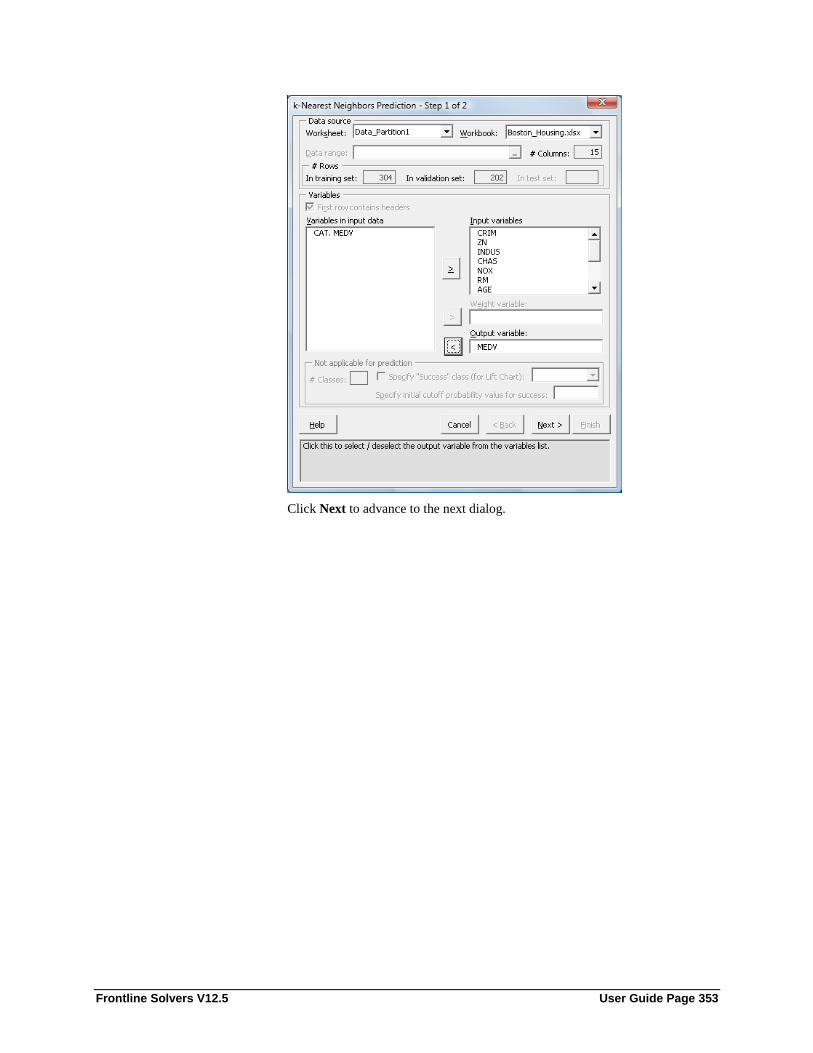
Frontline Solvers V12.5 User Guide Page 353
Click Next to advance to the next dialog.

Frontline Solvers V12.5 User Guide Page 354
Select Normalize Input data. When this option is selected, the input data is
normalized which means that all data is expressed in terms of standard
deviations. This option is available to ensure that the distance measure is not
dominated by variables with a large scale.
Enter 5 for the Number of Nearest Neighbors. This is the parameter k in the k-
nearest neighbor algorithm. The value of k should be between 1 and the total
number of observations (rows). Typically, this is chosen to be in units of tens.
Select Score on best k between 1 and specified value for the Scoring option.
XLMiner will display the output for the best k between 1 and 5. If Score on
specified value of k as above is selected, the output will be displayed for the
specified value of k.
Select Detailed scoring, Summary report, and Lift charts under both Score
training data and Score validation data to show an assessment of the
performance in predicting the training data.
The options in the Score test data group are enabled only when a test partition is
available.
Please see the Scoring chapter for a complete discussion on the options under
Score New Data.
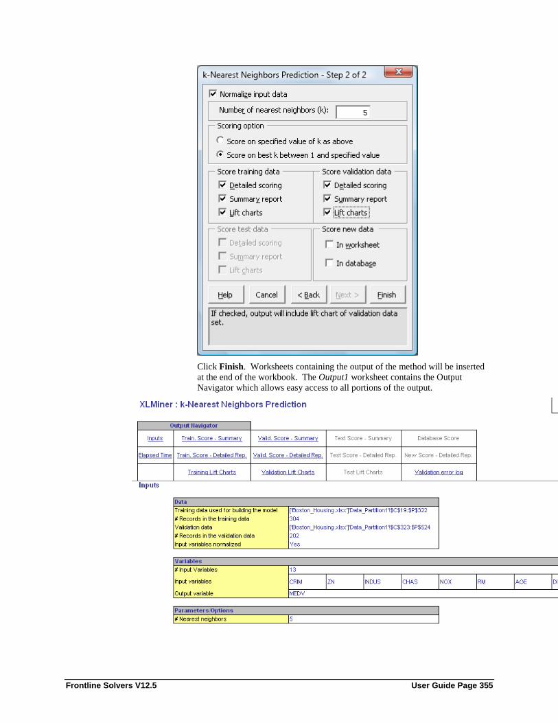
Frontline Solvers V12.5 User Guide Page 355
Click Finish. Worksheets containing the output of the method will be inserted
at the end of the workbook. The Output1 worksheet contains the Output
Navigator which allows easy access to all portions of the output.
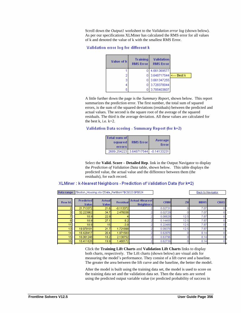
Frontline Solvers V12.5 User Guide Page 356
Scroll down the Output1 worksheet to the Validation error log (shown below).
As per our specifications XLMiner has calculated the RMS error for all values
of k and denoted the value of k with the smallest RMS Error.
A little further down the page is the Summary Report, shown below. This report
summarizes the prediction error. The first number, the total sum of squared
errors, is the sum of the squared deviations (residuals) between the predicted and
actual values. The second is the square root of the average of the squared
residuals. The third is the average deviation. All these values are calculated for
the best k, i.e. k=2.
Select the Valid. Score – Detailed Rep. link in the Output Navigator to display
the Prediction of Validation Data table, shown below. This table displays the
predicted value, the actual value and the difference between them (the
residuals), for each record.
Click the Training Lift Charts and Validation Lift Charts links to display
both charts, respectively. The Lift charts (shown below) are visual aids for
measuring the model’s performance. They consist of a lift curve and a baseline.
The greater the area between the lift curve and the baseline, the better the model.
After the model is built using the training data set, the model is used to score on
the training data set and the validation data set. Then the data sets are sorted
using the predicted output variable value (or predicted probability of success in

Frontline Solvers V12.5 User Guide Page 357
the logistic regression case). After sorting, the actual outcome values of the
output variable are cumulated and the lift curve is drawn as the number of cases
versus the cumulated value. The baseline is drawn as the number of cases
versus the average of actual output variable values multiplied by the number of
cases. The decilewise lift curve is drawn as the decile number versus the
cumulative actual output variable value divided by the decile's average output
variable value.
See the Scoring chapter for information on the KNNP_Stored_1 worksheet.
k-Nearest Neighbors Prediction Method Options The following options appear on the two k-Nearest Neighbors dialogs.

Frontline Solvers V12.5 User Guide Page 358
Variables in input data
All variables in the dataset are listed here.
Input variables
Variables listed here will be utilized in the XLMiner output.
Output Variable
Select the variable whose outcome is to be predicted here.

Frontline Solvers V12.5 User Guide Page 359
Normalize Input data
When this option is selected, the input data is normalized which means that all
data is expressed in terms of standard deviations. This option is available to
ensure that the distance measure is not dominated by variables with a large
scale. This option is not selected by default.
Number of Nearest Neighbors
This is the parameter k in the k-nearest neighbor algorithm. The value of k
should be between 1 and the total number of observations (rows). Typically, this
is chosen to be in units of tens. The default value is 1.
Scoring Option
When Score on best k between 1 and specified value is selected, XLMiner will
display the output for the best k between 1 and the value entered for Number of
nearest neighbors (k). If Score on specified value of k as above is selected, the
output will be displayed for the specified value of k. The default setting is Score
on specified value of k.
Score training data
Select these options to show an assessment of the performance of the tree in
classifying the training data. The report is displayed according to your
specifications - Detailed, Summary and Lift charts.

Frontline Solvers V12.5 User Guide Page 360
Score validation data
Select these options to show an assessment of the performance of the tree in
classifying the validation data. The report is displayed according to your
specifications - Detailed, Summary and Lift charts.
Score test data
These options are enabled when a test set is present. Select these options to
show an assessment of the performance of the tree in classifying the test data.
The report is displayed according to your specifications - Detailed, Summary
and Lift charts.
Score New Data See the Scoring chapter for more details on the In worksheet or In database
options.

Frontline Solvers V12.5 User Guide Page 361
Regression Tree Prediction Method
Introduction As with all regression techniques, XLMiner assumes the existence of a single
output (response) variable and one or more input (predictor) variables. The
output variable is numerical. The general regression tree building methodology
allows input variables to be a mixture of continuous and categorical variables.
A decision tree is generated where each decision node in the tree contains a test
on some input variable's value. The terminal nodes of the tree contain the
predicted output variable values.
A Regression tree may be considered as a variant of decision trees, designed to
approximate real-valued functions instead of being used for classification
methods.
Methodology
A Regression tree is built through a process known as binary recursive
partitioning. This is an iterative process that splits the data into partitions or
“branches”, and then continues splitting each partition into smaller groups as the
method moves up each branch.
Initially, all records in the training set (the pre-classified records that are used to
determine the structure of the tree) are grouped into the same partition. The
algorithm then begins allocating the data into the first two partitions or
“branches”, using every possible binary split on every field. The algorithm
selects the split that minimizes the sum of the squared deviations from the mean
in the two separate partitions. This splitting “rule” is then applied to each of the
new branches. This process continues until each node reaches a user-specified
minimum node size and becomes a terminal node. (If the sum of squared
deviations from the mean in a node is zero, then that node is considered a
terminal node even if it has not reached the minimum size.)
Pruning the tree
Since the tree is grown from the training data set, a fully developed tree
typically suffers from over-fitting (i.e. it is "explaining" random elements of the
training data that are not likely to be features of the larger population). This
over-fitting results in poor performance on “real life” data. Therefore, the tree
must be “pruned” using the validation data set. XLMiner calculates the cost
complexity factor at each step during the growth of the tree and decides the
number of decision nodes in the pruned tree. The cost complexity factor is the
multiplicative factor that is applied to the size of the tree (which is measured by
the number of terminal nodes).

Frontline Solvers V12.5 User Guide Page 362
The tree is pruned to minimize the sum of (1) the output variable variance in the
validation data, taken one terminal node at a time, and (2) the product of the cost
complexity factor and the number of terminal nodes. If the cost complexity
factor is specified as zero then pruning is simply finding the tree that performs
best on validation data in terms of total terminal node variance. Larger values of
the cost complexity factor result in smaller trees. Pruning is performed on a “last
in first out” basis meaning the last grown node is the first to be subject to
elimination.
Regression Tree Example This example illustrates XLMiner’s Regression Tree prediction method. We
will again use the Boston_Housing.xlsx example dataset. This dataset contains
14 variables, the description of each is given in the table below. The dependent
variable MEDV is the median value of a dwelling. This objective of this
example is to predict the value of MEDV.
A portion of the dataset is shown below. The last variable, CAT. MEDV, is a
discrete classification of the MEDV variable and will not be used in this
example.
CRIM Per capita crime rate by town
ZN Proportion of residential land zoned for lots over
25,000 sq.ft.
INDUS Proportion of non-retail business acres per town
CHAS Charles River dummy variable (= 1 if tract bounds
river; 0 otherwise)
NOX Nitric oxides concentration (parts per 10 million)
RM Average number of rooms per dwelling
AGE Proportion of owner-occupied units built prior to
1940
DIS Weighted distances to five Boston employment
centers
RAD Index of accessibility to radial highways
TAX Full-value property-tax rate per $10,000
PTRATIO Pupil-teacher ratio by town
B 1000(Bk - 0.63)^2 where Bk is the proportion of
African-Americans by town
LSTAT % Lower status of the population
MEDV Median value of owner-occupied homes in $1000's

Frontline Solvers V12.5 User Guide Page 363
First, we partition the data into training and validation sets using the Standard
Data Partition with percentages of 50% of the data randomly allocated to the
Training Set and 30% of the data randomly allocated to the Validation Set and
20% of the data randomly allocated to the Test Set (default settings for Specify
percentages). For more information on partitioning a dataset, see the Data
Mining Partitioning chapter.
Select a cell on the Data_Partition1 worksheet, then click Predict – Regression
Tree to open the following dialog.

Frontline Solvers V12.5 User Guide Page 364
Select MEDV as the Output variable, then select the remaining variables
(except CAT.MEDV) as the Input variables. (The Weight variable and the
Classes group are not used in the Regression Tree predictive method.)

Frontline Solvers V12.5 User Guide Page 365
Click Next to advance to the Step 2 of 3 dialog.
Leave Normalize input data option unchecked. Normalizing the data only makes
a difference if linear combinations of the input variables are used for splitting.
Enter 100 for the Maximum #splits for input variables. This is the maximum
number of splits allowed for each input variable.
Enter 25 for the Minimum #records in a terminal node. The tree will continue to
“grow” until all terminal nodes reach this size.
Select Using Best prune tree for the Scoring option. The option, Maximum
#decision nodes is enabled when Using user specified tree is selected.

Frontline Solvers V12.5 User Guide Page 366
Select Next to advance to the Step 3 of 3 dialog.
Enter 7 for the Maximum # levels to be displayed or the number of levels to be
displayed in the output file.
Select Full tree (grown using training data) to display the full regression tree
grown using the training dataset.

Frontline Solvers V12.5 User Guide Page 367
Select Pruned tree (pruned using validation data) to display the tree pruned
using the validation dataset.
Select Minimum error tree (pruned using validation data) to display the
minimum error tree, pruned using the validation dataset.
Select Detailed report, Summary report, and Lift charts under Score training
data, Score validation data, and Score test data to display each in the output.
See the Scoring chapter for details on scoring to a worksheet or database.
Click Finish. Worksheets containing the output of the method will be inserted
at the end of the workbook. The Output1 worksheet contains the Output
Navigator which allows easy access to all portions of the output.
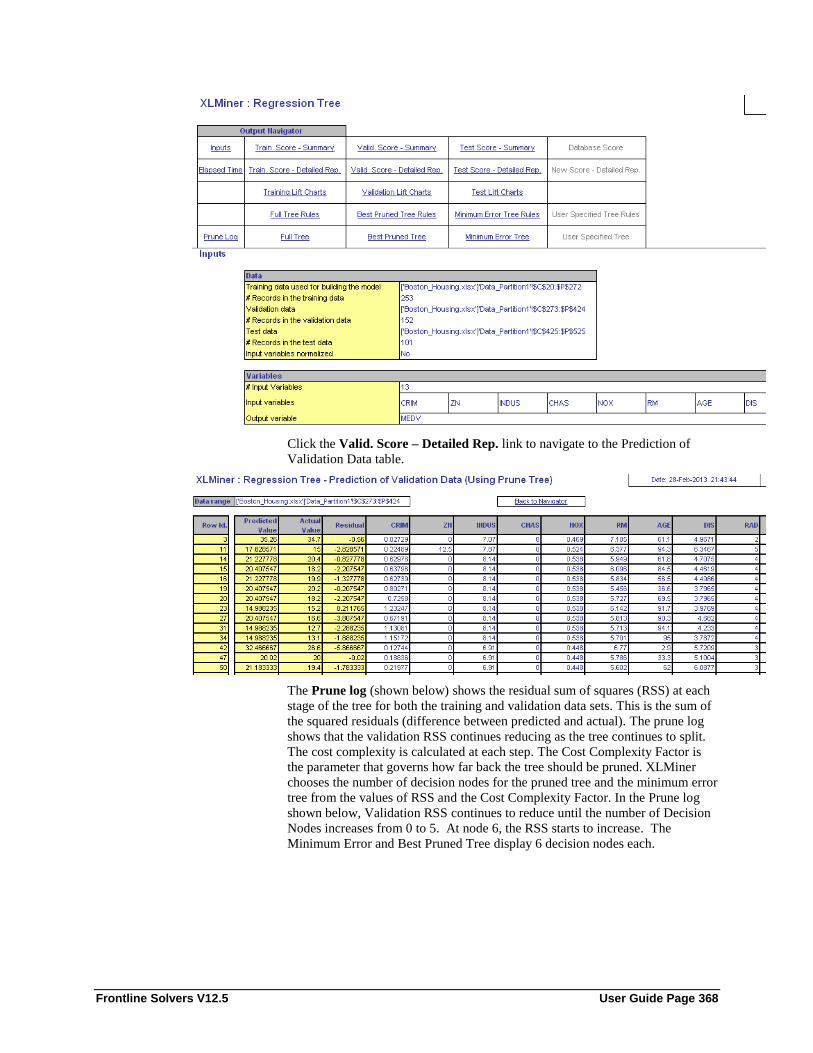
Frontline Solvers V12.5 User Guide Page 368
Click the Valid. Score – Detailed Rep. link to navigate to the Prediction of
Validation Data table.
The Prune log (shown below) shows the residual sum of squares (RSS) at each
stage of the tree for both the training and validation data sets. This is the sum of
the squared residuals (difference between predicted and actual). The prune log
shows that the validation RSS continues reducing as the tree continues to split.
The cost complexity is calculated at each step. The Cost Complexity Factor is
the parameter that governs how far back the tree should be pruned. XLMiner
chooses the number of decision nodes for the pruned tree and the minimum error
tree from the values of RSS and the Cost Complexity Factor. In the Prune log
shown below, Validation RSS continues to reduce until the number of Decision
Nodes increases from 0 to 5. At node 6, the RSS starts to increase. The
Minimum Error and Best Pruned Tree display 6 decision nodes each.

Frontline Solvers V12.5 User Guide Page 369
Click the Best Pruned Tree link to display the Best Pruned Tree (shown
below).

Frontline Solvers V12.5 User Guide Page 370
We can read this tree as follows. LSTAT (% of the population that is lower
status) is chosen as the first splitting variable; if this percentage is > 9.54 (95
cases), then LSTAT is again chosen for splitting. Now, if LSTAT <=14.98 (36
cases) then MEDV is predicted as $20.96. So the first rule is if LSTAT >9.54
and LSTAT<=14.895 then MEDV=$20.96.
If LSTAT <= 9.54%, then we move to RM (Average No. of rooms per dwelling)
as the next divider. If RM >7.141 (12 cases), MEDV for those cases is predicted
to be $40.69 ($40.69 is a terminal node). So the second rule is "If LSTAT <=
9.54 AND RM >7.141, then MEDV = $40.69."
The output also contains summary reports on both the training data and the
validation data. These reports contain the total sum of squared errors, the root
mean square error (RMS error, or the square root of the mean squared error),
and also the average error (which is much smaller, since errors fall roughly into
negative and positive errors and tend to cancel each other out unless squared
first.)
Select the Training Lift Charts and Validation Lift Charts links to navigate to
each. Lift charts are visual aids for measuring model performance. They consist
of a lift curve and a baseline. The larger the area between the lift curve and the
baseline, the better the model.
After the model is built using the training data set, the model is used to score on
the training data set and the validation data set. Then the data sets are sorted
using the predicted output variable value. After sorting, the actual outcome
values of the output variable are cumulated and the lift curve is drawn as the

Frontline Solvers V12.5 User Guide Page 371
number of cases versus the cumulated value. The baseline is drawn as the
number of cases versus the average of actual output variable values multiplied
by the number of cases. The decilewise lift curve is drawn as the decile number
versus the cumulative actual output variable value divided by the decile's
average output variable value.
For information on the RT_Stored_1 worksheet, please see the Scoring chapter.
Regression Tree Options The options below appear on one of the three Regression Tree dialogs.

Frontline Solvers V12.5 User Guide Page 372
Variables in input data
All variables in the dataset are listed here.
Input variables
Variables listed here will be utilized in the XLMiner output.
Weight Variable
The Weight variable is not used in this method.
Output Variable
Select the variable whose outcome is to be predicted here.

Frontline Solvers V12.5 User Guide Page 373
Normalize input data
When this option is checked, XLMiner will normalize the data. Normalizing the
data (subtracting the mean and dividing by the standard deviation) is important
to ensure that the distance measure accords equal weight to each variable --
without normalization, the variable with the largest scale will dominate the
measure. Normalizing the data will only make a difference if linear
combinations of the input variables are used for determining the splits. This
option is not selected by default.
Maximum # splits for input variables
This is the maximum number of splits allowed for each input variable. The
default setting is 100.
Minimum #records in a terminal node
The tree will continue to “grow” until all terminal nodes contain this number of
records. The default setting is 25.
Scoring option
Select the tree to be used for scoring. Select Using Full tree (the default) to use
the full grown tree for scoring. Select Using Best prune tree to use the best
pruned tree for scoring. Select Using minimum error tree to use the minimum
error tree for scoring. Select Using user specified tree to use a tree specified by
the user. The option, Maximum #decision nodes in the pruned tree, is enabled
when Using user specified tree is selected.

Frontline Solvers V12.5 User Guide Page 374
Maximum #levels to be displayed
Enter the desired number of nodes to be displayed in the output here. The
default value is 5.
Full tree (grown using training data)
Select this option to display the full regression tree. The tree will be drawn
according to the maximum #levels in the tree that are specified. This option is
not selected by default.
Pruned tree (pruned using validation data)
Select this option to display the pruned tree. This option is not selected by
default.
Minimum error tree (pruned using validation data)
Select this option to display the minimum error tree, pruned using validation
data. This option is not selected by default.

Frontline Solvers V12.5 User Guide Page 375
Score training data
Select these options to show an assessment of the performance of the tree in
classifying the training data. The report is displayed according to your
specifications - Detailed, Summary and Lift charts.
Score validation data
Select these options to show an assessment of the performance of the tree in
classifying the validation data. The report is displayed according to your
specifications - Detailed, Summary and Lift charts.
Score Test Data
Select these options to show an assessment of the performance of the tree in
classifying the test data. The report is displayed according to your specifications
- Detailed, Summary and Lift charts.
Score new Data
The options in this group let you apply the model for scoring to an altogether
new data. See the Scoring chapter for details on these options.

Frontline Solvers V12.5 User Guide Page 376
Neural Networks Prediction Method
Introduction Artificial neural networks are relatively crude electronic networks of "neurons"
based on the neural structure of the brain. They process records one at a time,
and "learn" by comparing their prediction of the record (which, at the outset, is
largely arbitrary) with the known actual record. The errors from the initial
prediction of the first record is fed back to the network and used to modify the
network’s algorithm for the second iteration. These steps are repeated multiple
times.
Roughly speaking, a neuron in an artificial neural network is
1. A set of input values (xi) with associated weights (wi)
2. A input function (g) that sums the weights and maps the results to an output
function(y).
Neurons are organized into layers: input, hidden and output. The input layer is
composed not of full neurons, but simply of the values in a record that are inputs
to the next layer of neurons. The next layer is the hidden layer of which there
could be several. The final layer is the output layer, where there is one node for
each class. A single sweep forward through the network results in the
assignment of a value to each output node. The record is assigned to the class
node with the highest value.

Frontline Solvers V12.5 User Guide Page 377
Training an Artificial Neural Network
In the training phase, the correct class for each record is known (this is termed
supervised training), and the output nodes can therefore be assigned "correct"
values -- "1" for the node corresponding to the correct class, and "0" for the
others. (In practice, better results have been found using values of “0.9” and
“0.1”, respectively.) As a result, it is possible to compare the network's
calculated values for the output nodes to these "correct" values, and calculate an
error term for each node. These error terms are then used to adjust the weights in
the hidden layers so that, hopefully, the next time around the output values will
be closer to the "correct" values.
The Iterative Learning Process
A key feature of neural networks is an iterative learning process in which
records (rows) are presented to the network one at a time, and the weights
associated with the input values are adjusted each time. After all cases are
presented, the process often starts over again. During this learning phase, the
network “trains” by adjusting the weights to predict the correct class label of
input samples. Advantages of neural networks include their high tolerance to
noisy data, as well as their ability to classify patterns on which they have not
been trained. The most popular neural network algorithm is the back-
propagation algorithm proposed in the 1980's.
Once a network has been structured for a particular application, that network is
ready to be trained. To start this process, the initial weights (described in the
next section) are chosen randomly. Then the training, or learning, begins.
The network processes the records in the training data one at a time, using the
weights and functions in the hidden layers, then compares the resulting outputs
against the desired outputs. Errors are then propagated back through the system,
causing the system to adjust the weights for the next record. This process occurs
over and over as the weights are continually tweaked. During the training of a
network the same set of data is processed many times as the connection weights
are continually refined.

Frontline Solvers V12.5 User Guide Page 378
Note that some networks never learn. This could be because the input data do
not contain the specific information from which the desired output is derived.
Networks also will not converge if there is not enough data to enable complete
learning. Ideally, there should be enough data available to create a validation set.
Feedforward, Back-Propagation
The feedforward, back-propagation architecture was developed in the early
1970's by several independent sources (Werbor; Parker; Rumelhart, Hinton and
Williams). This independent co-development was the result of a proliferation of
articles and talks at various conferences which stimulated the entire industry.
Currently, this synergistically developed back-propagation architecture is the
most popular, effective, and easy-to-learn model for complex, multi-layered
networks. Its greatest strength is in non-linear solutions to ill-defined problems.
The typical back-propagation network has an input layer, an output layer, and at
least one hidden layer. Theoretically, there is no limit on the number of hidden
layers but typically there are just one or two. Some studies have shown that the
total number of layers needed to solve problems of any complexity is 5 (one
input layer, three hidden layers and an output layer). Each layer is fully
connected to the succeeding layer.
As noted above, the training process normally uses some variant of the Delta
Rule, which starts with the calculated difference between the actual outputs and
the desired outputs. Using this error, connection weights are increased in
proportion to the error times, which are a scaling factor for global accuracy. This
means that the inputs, the output, and the desired output all must be present at
the same processing element. The most complex part of this algorithm is
determining which input contributed the most to an incorrect output and how to
modify the input to correct the error. (An inactive node would not contribute to
the error and would have no need to change its weights.) To solve this problem,
training inputs are applied to the input layer of the network, and desired outputs
are compared at the output layer. During the learning process, a forward sweep
is made through the network, and the output of each element is computed layer
by layer. The difference between the output of the final layer and the desired
output is back-propagated to the previous layer(s), usually modified by the
derivative of the transfer function. The connection weights are normally
adjusted using the Delta Rule. This process proceeds for the previous layer(s)
until the input layer is reached.
Structuring the Network
The number of layers and the number of processing elements per layer are
important decisions. These parameters, to a feedforward, back-propagation
topology, are also the most ethereal - they are the "art" of the network designer.
There is no quantifiable, best answer to the layout of the network for any
particular application. There are only general rules picked up over time and
followed by most researchers and engineers applying this architecture to their
problems.
Rule One: As the complexity in the relationship between the input data and the
desired output increases, the number of the processing elements in the hidden
layer should also increase.
Rule Two: If the process being modeled is separable into multiple stages, then
additional hidden layer(s) may be required. If the process is not separable into
stages, then additional layers may simply enable memorization of the training
set, and not a true general solution.

Frontline Solvers V12.5 User Guide Page 379
Rule Three: The amount of training data available sets an upper bound for the
number of processing elements in the hidden layer(s). To calculate this upper
bound, use the number of cases in the training data set and divide that number
by the sum of the number of nodes in the input and output layers in the network.
Then divide that result again by a scaling factor between five and ten. Larger
scaling factors are used for relatively less noisy data. If too many artificial
neurons are used the training set will be memorized, not generalized, and the
network will be useless on new data sets.
portion of the dataset is shown below. The last variable, CAT.MEDV, is a
discrete classification of the MEDV variable and will not be used in this
example.
Neural Network Prediction Method Example The example below illustrates XLMiner’s Neural Network Prediction method.
We will again use the Boston_Housing.xlsx example dataset. This dataset
contains 14 variables, the description of each is given in the table below. The
dependent variable MEDV is the median value of a dwelling. This objective of
this example is to predict the value of MEDV.
A portion of the dataset is shown below. The last variable, CAT.MEDV, is a
discrete classification of the MEDV variable and will not be used in this
example.
CRIM Per capita crime rate by town
ZN Proportion of residential land zoned for lots over
25,000 sq.ft.
INDUS Proportion of non-retail business acres per town
CHAS Charles River dummy variable (= 1 if tract bounds
river; 0 otherwise)
NOX Nitric oxides concentration (parts per 10 million)
RM Average number of rooms per dwelling
AGE Proportion of owner-occupied units built prior to
1940
DIS Weighted distances to five Boston employment
centers
RAD Index of accessibility to radial highways
TAX Full-value property-tax rate per $10,000
PTRATIO Pupil-teacher ratio by town
B 1000(Bk - 0.63)^2 where Bk is the proportion of
African-Americans by town
LSTAT % Lower status of the population
MEDV Median value of owner-occupied homes in $1000's

Frontline Solvers V12.5 User Guide Page 380
First, we partition the data into training and validation sets using the Standard
Data Partition defaults with percentages of 60% of the data randomly allocated
to the Training Set and 40% of the data randomly allocated to the Validation
Set. For more information on partitioning a dataset, see the Data Mining
Partitioning chapter.
Select a cell on the newly created Data_Partition1 worksheet, then click Predict
– Neural Network on the XLMiner ribbon. The following dialog appears.

Frontline Solvers V12.5 User Guide Page 381
Select Type as the Output variable and the remaining variables as Input
Variables (except the CAT.MEDV variable) Since the Output variable contains
three classes (A, B, and C) to denote the three different wineries, the options for
Classes in the output variable are disabled.
The Weight variable and the Success options are not used in this method and are
therefore not enabled.

Frontline Solvers V12.5 User Guide Page 382
Click Next to advance to the next dialog.
This dialog contains the options to define the network architecture. Keep
Normalize input data unselected in this example. Normalizing the data
(subtracting the mean and dividing by the standard deviation) is important to
ensure that the distance measure accords equal weight to each variable --
without normalization, the variable with the largest scale would dominate the
measure.
Keep the # Hidden Layers at the default value of 1. Click the up arrow to
increase the number of hidden layers. The default setting is 1. XLMiner
supports up to 4 hidden layers.
Enter 25 for the # Nodes for the Hidden layer.

Frontline Solvers V12.5 User Guide Page 383
Enter 500 for # Epochs. An epoch is one sweep through all records in the
training set.
Keep the default setting of 0.1 for Step size for gradient descent. This is the
multiplying factor for the error correction during backpropagation; it is roughly
equivalent to the learning rate for the neural network. A low value produces
slow but steady learning, a high value produces rapid but erratic learning.
Values for the step size typically range from 0.1 to 0.9.
Keep the default setting of 0.6 for Weight change momentum. In each new
round of error correction, some memory of the prior correction is retained so
that an outlier does not spoil accumulated learning.
Keep the default setting of 0.01 for Error tolerance. The error in a particular
iteration is backpropagated only if it is greater than the error tolerance. Typically
error tolerance is a small value in the range from 0 to 1.
Keep the default setting of 0 for Weight decay. To prevent over-fitting of the
network on the training data, set a weight decay to penalize the weight in each
iteration. Each calculated weight will be multiplied by 1-decay.
Click Next to advance to the Step 3 of 3 dialog.

Frontline Solvers V12.5 User Guide Page 384
Select Detailed report, Summary report, and Lift charts under Score training
data and Score validation data to show an assessment of the performance of the
tree in predicting the output variable. The output is displayed according to the
user’s specifications – Detailed, Summary, and/or Lift charts.
If a test dataset exists, the options under Score test data will be enabled. Select
Detailed report, Summary report, and Lift charts under Score test data to show
an assessment of the performance of the test dataset in predicting the output
variable. The output is displayed according to the user’s specifications –
Detailed, Summary, and/or Lift charts.
See the Scoring chapter for information on options under Score new data.
Click Finish to initiate the output. Worksheets containing the output of the
model will be inserted at the end of the workbook. The Output Navigator
appears on the NNP_Output1 worksheet. Click any link to easily view the
results.
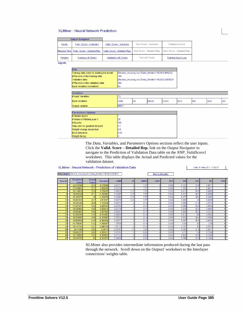
Frontline Solvers V12.5 User Guide Page 385
The Data, Variables, and Parameters Options sections reflect the user inputs.
Click the Valid. Score – Detailed Rep. link on the Output Navigator to
navigate to the Prediction of Validation Data table on the NNP_ValidScore1
worksheet. This table displays the Actual and Predicted values for the
validation dataset.
XLMiner also provides intermediate information produced during the last pass
through the network. Scroll down on the Output1 worksheet to the Interlayer
connections' weights table.

Frontline Solvers V12.5 User Guide Page 386
Recall that a key element in a neural network is the weights for the connections
between nodes. In this example, we chose to have one hidden layer, and we also
chose to have 25 nodes in that layer. XLMiner's output contains a section that
contains the final values for the weights between the input layer and the hidden
layer, between hidden layers, and between the last hidden layer and the output
layer. This information is useful at viewing the “insides” of the neural network;
however, it is unlikely to be of utility to the data analyst end-user. Displayed
above are the final connection weights between the input layer and the hidden
layer for our example.
Click the Training Epoch Log link on the Output Navigator to display the
following log.
During an epoch, each training record is fed forward in the network and
classified. The error is calculated and is back propagated for the weights
correction. As a result, weights are continuously adjusted during the epoch. The

Frontline Solvers V12.5 User Guide Page 387
classification error is computed as the records pass through the network. It does
not report the classification error after the final weight adjustment. Scoring of
the training data is performed using the final weights so the training
classification error may not exactly match with the last epoch error in the Epoch
log.
See the Scoring chapter for information on the Stored Model Sheet,
NNC_Stored_1.
Neural Network Prediction Method Options The options below appear on one of the three Neural Network Prediction
method dialogs.
Variables in input data
All variables in the dataset are listed here.
Input variables
Variables listed here will be utilized in the XLMiner output.
Weight Variable
The Weight variable is not used in this method.

Frontline Solvers V12.5 User Guide Page 388
Output Variable
Select the variable whose outcome is to be predicted here.
Normalize input data
Normalizing the data (subtracting the mean and dividing by the standard
deviation) is important to ensure that the distance measure accords equal weight
to each variable -- without normalization, the variable with the largest scale
would dominate the measure. This option is not selected by default.
# Hidden Layers
Click the up and down arrows until the desired number of hidden layers appears.
The default setting is 1. XLMiner supports up to 4 hidden layers.
# Nodes
Enter the number of nodes per layer here. The first field is for the first hidden
layer, the second field is for the second hidden layer, etc.
# Epochs
An epoch is one sweep through all records in the training set. The default
setting is 30.
Step size for gradient descent
This is the multiplying factor for the error correction during backpropagation; it
is roughly equivalent to the learning rate for the neural network. A low value
produces slow but steady learning, a high value produces rapid but erratic
learning. Values for the step size typically range from 0.1 to 0.9. The default
setting is 0.1.

Frontline Solvers V12.5 User Guide Page 389
Weight change momentum
In each new round of error correction, some memory of the prior correction is
retained so that an outlier that crops up does not spoil accumulated learning.
The default setting is 0.6.
Error tolerance
The error in a particular iteration is backpropagated only if it is greater than the
error tolerance. Typically error tolerance is a small value in the range from 0 to
1. The default setting is 0.01.
Weight decay
To prevent over-fitting of the network on the training data, set a weight decay to
penalize the weight in each iteration. Each calculated weight will be multiplied
by (1-decay). The default setting is 0.
Score training data
Select these options to show an assessment of the performance of the tree in
predicting the output variable using the training data. The report is displayed
according to your specifications - Detailed, Summary and Lift charts.
Score validation data
Select these options to show an assessment of the performance of the tree in
predicting the value of the output variable using the validation data. The report
is displayed according to your specifications - Detailed, Summary and Lift
charts.

Frontline Solvers V12.5 User Guide Page 390
Score Test Data
Select these options to show an assessment of the performance of the tree in
predicting the output variable using the test data. The report is displayed
according to your specifications - Detailed, Summary and Lift charts.
Score new Data
The options in this group apply the model to be scored to an altogether new
dataset. See the Scoring chapter for details on these options.

Frontline Solvers V12.5 User Guide Page 391
Association Rules
Introduction The goal of association rule mining is to recognize associations and/or
correlations among large sets of data items. A typical and widely-used example
of association rule mining is the Market Basket Analysis. Most ‘market basket’
databases consist of a large number of transaction records where each record
lists all items purchased by a customer during a trip through the check-out line.
Data is easily and accurately collected through the bar-code scanners.
Supermarket managers are interested in determining what foods customers
purchase together, like, for instance, bread and milk, bacon and eggs, wine and
cheese, etc. This information is useful in planning store layouts (placing items
optimally with respect to each other), cross-selling promotions, coupon offers,
etc.
Association rules provide results in the form of "if-then" statements. These rules
are computed from the data and, unlike the if-then rules of logic, are
probabilistic in nature. The “if” portion of the statement is referred to as the
antecedent and the “then” portion of the statement is referred to as the
consequent.
In addition to the antecedent (the "if" part) and the consequent (the "then" part),
an association rule contains two numbers that express the degree of uncertainty
about the rule. In association analysis the antecedent and consequent are sets of
items (called itemsets) that are disjoint meaning they do not have any items in
common. The first number is called the support which is simply the number of
transactions that include all items in the antecedent and consequent. (The
support is sometimes expressed as a percentage of the total number of records in
the database.) The second number is known as the confidence which is the ratio
of the number of transactions that include all items in the consequent as well as
the antecedent (namely, the support) to the number of transactions that include
all items in the antecedent. For example, assume a supermarket database has
100,000 point-of-sale transactions, out of which 2,000 include both items A and
B and 800 of these include item C. The association rule "If A and B are
purchased then C is purchased on the same trip" has a support of 800
transactions (alternatively 0.8% = 800/100,000) and a confidence of 40%
(=800/2,000). In other works, support is the probability that a randomly selected
transaction from the database will contain all items in the antecedent and the
consequent. Confidence is the conditional probability that a randomly selected
transaction will include all the items in the consequent given that the transaction
includes all the items in the antecedent.
Lift is one more parameter of interest in the association analysis. Lift is the ratio
of Confidence to Expected Confidence. Expected Confidence, in the example
above, is the "confidence of buying A and B does not enhance the probability of
buying C." or the number of transactions that include the consequent divided by
the total number of transactions. Suppose the total number of transactions for C
is 5,000. Expected Confidence is computed as 5% (5,000/1,000,000) while the
ratio of Lift Confidence to Expected Confidence is 8 (40%/5%). Hence, Lift is a

Frontline Solvers V12.5 User Guide Page 392
value that provides information about the increase in probability of the "then"
(consequent) given the "if" (antecedent).
A lift ratio larger than 1.0 implies that the relationship between the antecedent
and the consequent is more significant than would be expected if the two sets
were independent. The larger the lift ratio, the more significant the association.
Association Rule Example This example below illustrates XLMiner’s Association Rule method. Click
Help – Examples to open the Associations.xlsx example file. A portion of the
dataset is shown below.
Select a cell in the dataset, say, A2, then click Associate – Association Rules to
open the Association Rule dialog, shown below.
Since the data contained in the Associations.xlsx dataset are all 0’s and 1’s,
select Data in binary matrix format for the Input data format. This option
should be selected if each column in the data represents a distinct item.
XLMiner will treat the data as a matrix of two entities -- zeros and non-zeros.

Frontline Solvers V12.5 User Guide Page 393
All non-zeros are treated as 1's. A 0 signifies that the item is absent in that
transaction and a 1 signifies the item is present. Select Data in item list format
when each row of data consists of item codes or names that are present in that
transaction. Enter 100 for the Minimum Support (# transactions). This option
specifies the minimum number of transactions in which a particular item-set
must appear to qualify for inclusion in an association rule. Enter 90 for
Minimum confidence. This option specifies the minimum confidence threshold
for rule generation. If A is the set of Antecedents and C the set of Consequents,
then only those A =>C ("Antecedent implies Consequent") rules will qualify, for
which the ratio (support of A U C) / (support of A) at least equals this
percentage.
Click OK. The output worksheet, AssocRules_1, is inserted immediately after
the Assoc_binary worksheet. Click the column titles to sort each rule by
ascending or descending values.
Rule 2 indicates that if an Italian cookbook and a Youth book are purchased,
then with 100% confidence a second cookbook will also be purchased. Support
(a) indicates that the rule has support of all 118 transactions, meaning that 118
people bought an Italian cookbook and a Youth book. Support (c) indicates the
number of transactions involving the purchase of cookbooks. Support (a U c)

Frontline Solvers V12.5 User Guide Page 394
indicates the number of transactions where an Italian cookbook and a Youth
book as well as a second cookbook were purchased.
The Lift Ratio indicates how much more likely a transaction will be found
where an Italian cookbook and a Youth book are purchased, as compared to the
entire population of transactions. In other words, the Lift Ratio is the
confidence divided by support (c), where the latter is expressed as a percentage.
For Rule 2, with a confidence of 100%, support is calculated as 862/2000 * 100
= 43.1. Consequently, the Lift ratio is calculated as 100/43.1 or 2.320186.
Given support at 100% and a lift ratio of 2.320186, this rule can be considered
“useful”.
Association Rule Options The following options appear on the Association Rule dialog.
Input data format
Select Data in binary matrix format if each column in the data represents a
distinct item. If this option is selected, XLMiner treats the data as a matrix of
two entities -- zeros and non-zeros. All non-zeros are treated as 1's. So,
effectively the data set is converted to a binary matrix which contains 0's and 1's.
A 0 indicates that the item is absent in the transaction and a 1 indicates it is
present.
Select Input Data in item list format if each row of data consists of item codes
or names that are present in that transaction.
Minimum support (# transactions)
Specify the minimum number of transactions in which a particular item-set must
appear for it to qualify for inclusion in an association rule here. The default
setting is 200.

Frontline Solvers V12.5 User Guide Page 395
Minimum confidence (%)
A value entered for this option specifies the minimum confidence threshold for
rule generation. If A is the set of Antecedents and C the set of Consequents, then
only those A =>C ("Antecedent implies Consequent") rules will qualify, for
which the ratio (support of A U C) / (support of A) is greater than or equal to.
The default setting is 50.

Frontline Solvers V12.5 User Guide Page 396
Scoring New Data
Introduction XLMiner provides a method for scoring new data in a database or worksheet
with any of the Classification or Prediction algorithms. This facility matches the
input variables to the database (or worksheet) fields and then performs the
scoring on the database (or worksheet).
Scoring to a Database Refer to the Discriminant Analysis example in the previous chapter
Discriminant Analysis Classification Method for instructions on advancing to
the Discriminant Analysis Step 3 of 3 dialog. This feature can be used with any
of the Classification or Prediction algorithms and can be found on the last dialog
for each method. In the Discriminant Analysis method, this feature is found on
the Step 3 of 3 dialog.
In the Score new data in group, select Database. The Scoring to Database
dialog opens.

Frontline Solvers V12.5 User Guide Page 397
The first step on this dialog is to select the Data source. Once the Data source
is selected, Connect to a database… will be enabled.
If your database is a SQL Server database, select SQL Server for Data source
then click Connect to a database…, the following dialog will appear. Enter the
appropriate details, then click OK to be connected to the database.
If your data source is an Oracle database, select Oracle as Data source, then
click Connect to a database…, the following dialog will appear.
Enter the appropriate details and click OK to connect to the database.

Frontline Solvers V12.5 User Guide Page 398
This example illustrates how to score to an MS-Access database. Select MS-
Access for the Data source, then click Connect to a Database… The following
dialog appears.
Click Browse for database file… and browse to C:\Program Files\Frontline
Systems\Analytic Solver Platform\Datasets\dataset.mdb,
then click Open. The MS-Access database file dialog re-appears.

Frontline Solvers V12.5 User Guide Page 399
Click OK to close the MS-Access database file dialog. The Scoring to Database
dialog re-appears. Select Boston_Housing for Select table/view. The dialog
will be populated with variables from the database, dataset.mdb, under Fields in
table and with variables from the Boston_Housing.xlsx workbook under
Variables in input data.
XLMiner offers three easy techniques to match variables in the dataset to
variables in the database:
1. Matching variables with the same names.
2. Matching the first N variables where N is the number of input
variables.
3. Manually matching the variables.
If Match variable(s) with same names(s) is clicked, all similar named
variables in Boston_Housing.xlsx will be matched with similar named variables
in dataset.mdb, as shown in the screenprint below. Note that the additional
database fields remain in the Fields in table listbox while all variables in the
Variables in input data listbox have been matched.

Frontline Solvers V12.5 User Guide Page 400
If Match the first 11 variables in the same sequence is clicked, the first 11
variables in Boston_Housing.xlsx will be matched with the first 11 variables in
the dataset.mdb database.
The first 11 variables in both the database and the dataset are now matched
under Variables in input data. The additional database fields remain under
Fields in table.
Note: The 11 in Match the first 11 variables in the same sequence command
button title will change with the number of input variables.

Frontline Solvers V12.5 User Guide Page 401
To manually map variables from the dataset to the database, select a variable
from the database in the Fields in table listbox, then select the variable to be
matched in the dataset in the Variables in input data listbox, then click Match.
For example to match the CRIM variable in the database to the CRIM variable
in the dataset, select CRIM from the dataset.mdb database in the Fields in table
listbox, select CRIM from the Boston_Housing.xlsx dataset in the Variables in
input data listbox, then click Match CRIM < -- > CRIM to match the two
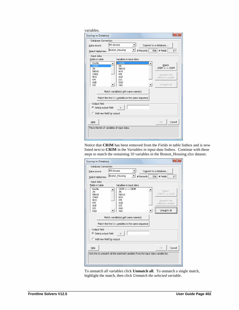
Frontline Solvers V12.5 User Guide Page 402
variables.
Notice that CRIM has been removed from the Fields in table listbox and is now
listed next to CRIM in the Variables in input data listbox. Continue with these
steps to match the remaining 10 variables in the Boston_Housing.xlsx dataset.
To unmatch all variables click Unmatch all. To unmatch a single match,
highlight the match, then click Unmatch the selected variable.

Frontline Solvers V12.5 User Guide Page 403
The Output Field can be selected from the remaining database fields listed under
Fields in table or a new Output Field can be added. Note: An output field
must be a string. To select an output field from the remaining database fields,
select the field to be added as the output field, in this case, nfld, then click > to
the right of the Select output field radio button.
In this example, the field nfld is the only remaining database field which is a
string so it is the only choice for the output field. To choose a different output
field click the < command button to return the nfld field to the Fields in table
listbox.
To add a new field for the output, select Add new field for output radio button,
then type a name for this new field such as “Output_Field”. XLMiner will
create the new field in the dataset.mdb database

Frontline Solvers V12.5 User Guide Page 404
After all the desired variables in the input data have been matched, OK will be
enabled, click to return to the original Step 3 of 3 dialog. Notice that Database
is selected.
Click Finish to create the scoring report on the DA_DBScore1 worksheet.

Frontline Solvers V12.5 User Guide Page 405
Scoring on New Data XLMiner can also perform scoring on new data in a worksheet. Click Help –
Examples on the XLMiner ribbon and open the Digit.xlsx and
Flying_Fitness.xlsx example datasets. Select a cell on the Data worksheet of
Flying_Fitness.xlsx workbook, say cell A2, and click Classify – Discriminant
Analysis to open the Discriminant Analysis Step 1 of 3 dialog.
Select Var2, Var3, Var4, Var5, and Var6 as the Input variables and
TestRes/Var1 as the Output variable.
Click Next to advance to the Step 2 of 3 dialog. Then click Next on the Step 2
of 3 dialog to accept the defaults.

Frontline Solvers V12.5 User Guide Page 406
On the Step 3 of 3 dialog, select Detailed report in the Score new data in group.
The dialog for Match variables in the new page appears.

Frontline Solvers V12.5 User Guide Page 407
Select Digits.xlsx for Workbook at the top of the dialog.
In the dialog above, the variables listed under Variables in new data are from
Digits.xlsx and the variables listed under Variables in input data are from
Flying_Fitness.xlsx. Again, variables can be matched in three different ways.
1. Match variables with same names.
2. Match the first N variables where N is the number of variables
included in the input data.
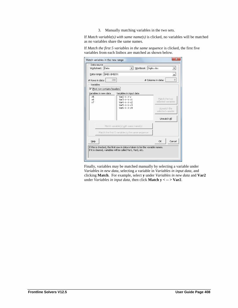
Frontline Solvers V12.5 User Guide Page 408
3. Manually matching variables in the two sets.
If Match variable(s) with same name(s) is clicked, no variables will be matched
as no variables share the same names.
If Match the first 5 variables in the same sequence is clicked, the first five
variables from each listbox are matched as shown below.
Finally, variables may be matched manually by selecting a variable under
Variables in new data, selecting a variable in Variables in input data, and
clicking Match. For example, select y under Variables in new data and Var2
under Variables in input data, then click Match y < -- > Var2.

Frontline Solvers V12.5 User Guide Page 409
Notice y has been removed from the Variables in new data listbox and added to
the Variables in input data listbox.
Continue these steps until all input variables are matched.

Frontline Solvers V12.5 User Guide Page 410
To unmatch all matched variables, click Unmatch all. To unmatch only one set
of matched variables, select the matched variables in the Variables in input data
listbox, then select Unmatch.
Click OK to return to the Step 3 of 3 dialog. Notice Detailed report is now
selected in the Score new data in group and Canonical Scores has been enabled
within that same group.
Click Finish to review the output. Click the DA_NewScore1 worksheet to view
the output as shown below. All variables in the input data have been matched

Frontline Solvers V12.5 User Guide Page 411
with the variables in the new data. Instead of Var2, y is listed, instead of Var3,
x1 is listed, instead of Var4, x2 is listed, etc.

Frontline Solvers V12.5 User Guide Page 412
Scoring Test Data
Introduction When XLMiner calculates prediction or classification results, internal values
and coefficients are generated and used in the computations. XLMiner saves
these values to an additional output sheet, termed Stored Model Sheet, which
uses the worksheet name, XX_Stored_N where XX are the initials of the
classification or prediction method and N is the number of generated stored
sheets. This sheet is used when scoring the test data. Note: In previous
versions of XLMiner, this utility was a separate add-on application named
XLMCalc. In XLMiner V12.5, this utility is included free of charge and can be
accessed under Score in the Tools section of the XLMiner ribbon.
The material saved to the Stored Model Sheet varies with the classification or
prediction method used. Please see the table below for details.
Classification/Prediction Method Contents of Stored Model Sheet
Multiple Linear or Logistic Regression Coefficients of the regression
equation.
Classification or Regression Trees Tree rules for all selected trees.
Naïve Bayes Each variable value, class and all
class probabilities.
k-Nearest Neighbors Model generated from training data.
Neural Networks All weights between Input, Hidden,
and Output layers
Discriminant Analysis Discriminant coefficients for each
class.
For example, assume the Multiple Linear Regression prediction method has just
finished. The Stored Model Sheet (MLR_Stored_1) will contain the regression
equation. When the Score Test Data utility is invoked, XLMiner will apply this
equation from the Stored Model Sheet to the test data.
Along with values required to generate the output, the Stored Model Sheet also
contains information associated with the input variables that were present in the
training data. The dataset on which the scoring will be performed should
contain at least these original Input variables. XLMiner offers a “matching”
utility that will match the Input variables in the training set to the variables in
the new dataset so the variable names are not required to be identical in both
data sets (training and test).

Frontline Solvers V12.5 User Guide Page 413
Scoring Test Data Example This example illustrates how to score test data using a stored model sheet using
output from a Multiple Linear Regression. This procedure may be repeated on
stored model sheets generated from the following Classification or Prediction
routines: Logistic Regression, k-Nearest Neighbors, Neural Networks, Naive
Bayes, or Discriminant Analysis.
Click Help – Examples on the XLMiner ribbon and open the example files,
Scoring.xlsm and Boston_Housing.xlsx. The Scoring.xlsm workbook contains
the MLR_Stored_1 worksheet which was generated by the Multiple Linear
Regression prediction routine on the Boston_Housing example dataset.
Select a cell on the Data worksheet within the Boston_Housing.xlsx workbook,
say A2, then click Score on the XLMiner ribbon. Under Data to be scored,
confirm that Data appears as the Worksheet and Boston_Housing.xlsx as the
Workbook.
Under Stored Model, select Scoring.xlsm for Workbook,
then MLR_Stored_1 under Worksheet.

Frontline Solvers V12.5 User Guide Page 414
Click Next. XLMiner will open the Match variables – Step 2 dialog which is
where the matching of the Input variables to the New Data variables will take
place.
XLMiner displays the list of variables on the Stored Model Sheet under
Variables in stored model and the variables in the new data under Variables in
new data.
Variables may be matched using three easy techniques: by name, by sequence
or manually.
If Match variable(s) with same names(s) is clicked, all similar named
variables in the stored model sheet will be matched with similar named variables
in the new dataset. However, since none of the variables in either list are named
similarly, no variables are “matched”.
If Match variables in stored model in same sequence is clicked, the Variables
in the stored model will be matched with the Variables in the new data in order
that they appear in the two listboxes. For example, the variable CRIM from the
new dataset will be matched with the variable CRIM_Scr from the stored model
sheet, the variable ZN from the new data will be matched with the variable
ZN_Scr from the stored model sheet and so on.

Frontline Solvers V12.5 User Guide Page 415
Since the stored model sheet only contains 13 variables while the new data
contains 15 variables, two variables will remain in the Variables in new data
listbox. Note: It is essential that the variables in the new data set appear in the
same sequence as the variables in the stored model when using this matching
technique.
To manually map variables from the stored model sheet to the new data set,
select a variable from the new data set in the Variables in new data listbox, then
select the variable to be matched in the stored model sheet in the Variables in
stored model listbox, then click Match. For example to match the CRIM
variable in the new dataset to the CRIM_Scr variable in the stored model sheet,
select CRIM from the Variables in new data listbox, select CRIM_Scr from
the stored model sheet in the Variables in stored model listbox, then click
Match CRIM < -- > CRIM to match the two variables.
Notice that CRIM has been removed from the Variables in new data listbox and
is now listed next to CRIM_SCR in the Variables in stored model listbox.
Continue with these steps to match the remaining 12 variables in the stored
model sheet.

Frontline Solvers V12.5 User Guide Page 416
To unmatch all variables click Unmatch all. To unmatch CRIM and
CRIM_SCR, click Unmatch CRIM_SCR <- -> CRIM.
For this example, click Match variables in stored model in same sequence to
match the variables in the new dataset to the variables on the stored model sheet.
Then click OK. A new sheet MLR_Score1 will be added to
Boston_Housing.xlsx. A portion of this output is shown below.
Now let’s apply these same steps to a stored model sheet created by the
Classification Tree classification method.
Click Score on the XLMiner ribbon. Confirm that Boston_Housing.xlsx is
selected for Workbook and Data is selected for Worksheet under Data to be
scored. Then, under Stored Model, select Scoring.xlsm for Workbook and
CT_Stored_1 for Worksheet.
Click Next to advance to the Step 2 dialog. Click Match variables in stored
model in same sequence.

Frontline Solvers V12.5 User Guide Page 417
Click Next to advance to the Step 3 dialog.
Click the down arrow to select the desired scoring option, then click OK. (Since
this stored model sheet was created when only the Full Tree Rules option was
selected during the Classification Tree method, this is the only option.) The
worksheet CT_Score1 will be added at the end of the workbook. A portion of
the output is shown below.

Frontline Solvers V12.5 User Guide Page 418
Scoring Test Data Options The options below appear on one of the Scoring Test Data dialogs.
Data to be Scored
Workbook: Select the open workbook containing the data to be scored here.
Worksheet: Select the worksheet, from the Workbook selection, containing the
data to be scored here.
Data Range: The dataset range will be prefilled here. If not prefilled, enter the
dataset range here.
First Row Contains Headers: This option is selected by default and indicates to
XLMiner to list variables in the Step 2 dialog by their column headings.
Stored Model
Workbook: Select the open workbook containing the Stored Model Sheet here.
Worksheet: Select the Stored Model worksheet, from the Workbook selection,
here.

Frontline Solvers V12.5 User Guide Page 419
XLMiner displays the list of variables on the Stored Model Sheet under
Variables in stored model and the variables in the new data under Variables in
new data.
Variables may be matched using three easy techniques: by name, by sequence,
or manually.
Match by Name
If Match variable(s) with same names(s) is clicked, all similar named
variables in the stored model sheet will be matched with similar named variables
in the new dataset. However, if none of the variables in either list are named
similarly, no variables will be “matched”.
Match by Sequence
If Match variables in stored model in same sequence is clicked, the Variables
in the stored model will be matched with the Variables in the new data in order
that they appear in the two listboxes. In the dialog above, the variable CRIM
from the new dataset will be matched with the variable CRIM_Scr from the
stored model sheet, the variable ZN from the new data will be matched with the
variable ZN_Scr from the stored model sheet and so on.
Manual Match
To manually map variables from the stored model sheet to the new data set,
select a variable from the new data set in the Variables in new data listbox, then
select the variable to be matched in the stored model sheet in the Variables in
stored model listbox, then click Match. To match the CRIM variable in the new
dataset to the CRIM_Scr variable in the stored model sheet in the dialog above,
select CRIM from the Variables in new data listbox, select CRIM_Scr from
the stored model sheet in the Variables in stored model listbox, then click
Match CRIM < -- > CRIM.

Frontline Solvers V12.5 User Guide Page 420
When scoring to a Stored Model Sheet generated by the Classification Tree
method, an additional dialog will appear. Click the down arrow to select the
desired scoring rule. The options appearing in this drop down are based on the
options selected on the Classification Tree Step 3 of 3 dialog.