Xrefs, Hatching and Raster Images: An AutoCAD® Survival Course Jennifer Leamy – Clough, Harbour & Associates LLP

GD405-2 Do visions of unreferenced Xrefs haunt you? Could a chicken hatch better than you? Does the thought of raster images make you break out in a cold sweat? If so, you’re not alone! Come join us in this exploration of Xrefs, hatching, and raster images. Learn the secrets of these simple yet complex commands and amaze your friends and coworkers ... or at least make your life a little easier.

About the Speaker: Jennifer is the AUGI Training Program manager and has taught 4 popular ATP courses (and counting). She is currently working at Clough Harbour and Associates, L.L.C., as a mechanical drafter. She has her Associate in Applied Science degree in Industrial Technology and has been an AutoCAD user since 1999. Jennifer has overseen upgrades, trained coworkers, and never tires of learning something new!

cadkitty@gmail.com

Xrefs, Hatching, and Raster Images: An AutoCAD® Survival Course

What is an Xref? If you look up xref in the AutoCAD help file, you first get redirected to “external reference”, and then find the following definition:

external reference (xref)

A drawing file referenced by another drawing. (XREF)

If your reaction was “Say what?!?”, trust me, you’re not alone! An external reference, or xref as they’re more commonly called, is a drawing. What makes it different is that it’s attached to another drawing in such a way that it appears to be in the drawing, but it’s really not. Got it? No? Good! Ok, picture this: you have a piece of paper with a floor plan on it – that’s your xref. Now, you lay a piece of tracing paper over the top of the floor plan – that’s your drawing. You can see the floor plan, you can draw over the top of it, but you can’t change it from the tracing paper. You have to go back to your original piece of paper to do that. Neat, huh?

When Should Xrefs be Used? Deciding when to use an xref is completely dependent upon you or your company. The broadest way I can think of to explain it is to say that they should be used anytime a floor plan, detail, section, schedule, etc. is going to be changing and needs to be used by multiple people or on multiple drawings.

Classic example: you’re an MEP firm working with an architect on a new building. They send you the floor plans for the project, and its common knowledge that they will change a bazillion times before you issue the final drawings. Now, four engineers each need their own drawings showing each of the three floors of the building, and they want two drawings showing the first floor, two showing the second floor, etc. Now then, do you a) want to go into 24 drawings every time the architect sends over updated plans and change the floor plans, b) want to change just three drawings every time the architect sends over updated plans, or c) want to break into the architecture firm and steal all electronic copies of the floor plans, thus making it impossible for them to ever change them.

The correct answer is, of course, ‘c’, but they wouldn’t let me teach a course on that (something about lawsuits and jail time), so the next closest correct answer is ‘b’.

Again, don’t think that xrefs are limited to floor plans – I’m just teaching what I know!

With that little disclaimer out of the way, let’s continue, shall we?

Creating an Xref Creating an xref is as simple as creating a drawing. Sticking with our example of floor plans received from an architect, you have two options – use the file they sent you exactly as it is, or adjust the drawing according to your company’s CAD standards and use that new file. For simplicity’s sake, we’ll say that you use the exact file that the architect sent you. An important thing to remember is that the plan must be in model space, not paper space.

Introducing the Xref Manager All right, so as with everything AutoCAD there is three ways to do this – toolbar, pull down menu, and keyboard entry – in this case, “xr”. All of these commands then bring up your new best friend – the Xref Manager Tool Palette.

Fig. 02

Xref Pulldown

Fig. 01

Xref Toolbar

Fig. 03

Xref Tool Palette

Attaching an Xref The highlighted button in Figure 03 is the xref attach command. Clicking on it brings up the screen shown in Figure 04.

Fig. 04 Attaching the Xref

Ok, as you can see in Figure 04, there are many choices here! Reference type, Path type, Insertion point, Scale, and Rotation. Let’s tackle these one at a time, shall we?

Reference Type You have two choices here – Attachment and Overlay. Attachment means just that – the xref is attached to the drawing. The only drawback is this: should you xref the drawing you’ve created, the xref already in there comes with it. Now then, most people want this to happen! If you’ve drawn a lighting layout over a floor plan, and you now want the take the whole thing and make it an xref for the utility plan, you want the floor plan to come along! If you don’t want this to happen, then use Overlay. All this does is keep the xref as a separate entity from the rest of the drawing. So now if you take that lighting plan and xref it into the utility plan, you won’t see the floor plan as it was simply overlaid.

Path Type Here you have three choices – full path (also called absolute path), relative path, or no path.

The full or absolute path specifies exactly where you should look for the xref. Referring back to Figure 04, you’ll see exactly where my x-flrpln1.dwg is located. The downside of this is if you move the folder your xrefs are located in to another drive, you have to go back and redefine all of the paths as AutoCAD will continue to look for it in the drive you specified. Now then, if you’re like my firm and keep all the xrefs in one place and never move the folder, then no problem! If, however, your conventions are different where you are, then one of the other two options should better suit your needs.

The relative path is considered more flexible as it does not require you to specify a drive letter. Instead, it simply assumes that the xref is located on the same drive as your drawing. If this is not true, you cannot use this option – AutoCAD won’t be able to find the xref! The benefit here is that you can move your set of drawings to a different drive (provided it has the same folder structure) without having to reset all of the xref paths. The conventions for specifying a relative folder path for the xref are as follows:

\

Look in the root folder of the host drawing's drive

path

From the folder of the host drawing, follow the specified path

\path

From the root folder, follow the specified path

.\path

From the folder of the host drawing, follow the specified path

..\path

From the folder of the host drawing, move up one folder level and follow the specified path

..\..\path

From the folder of the host drawing, move up two folder levels and follow the specified path

Should you select the no path option, AutoCAD then searches for the xref in the following order:

• Current folder of the host drawing • Project search paths defined on the Files tab in the Options dialog box and in the

PROJECTNAME system variable • Support search paths defined on the Files tab in the Options dialog box • Start In folder specified in the Windows application shortcut

If you select no path, your xref had better be in one of these places, otherwise AutoCAD will not be able to find it! This option is useful when moving the set of drawings to a different or unknown folder hierarchy.

Insertion Point Ok, ready? All together now – specifies the insertion point of the xref! As you can see in Figure 04, you have the choice of specifying the insertion point on the screen or right there in the dialog box. Should you choose to specify the insertion point in the dialog box and don’t want it to be located at 0,0,0, then you must specify the base point using the BASE command in the xref first. Personally, I just specify it on the screen. That way, I know exactly where it’s going to land instead of hoping that I chose the right base point and calculated the offset correctly. I like easy, don’t you?

Scale and Rotation Yes, I’m combining these two because they’re rather simple. You can specify the scale and rotation of the xref on the screen or in the dialog box. If you leave the scale as all 1’s as shown in Figure 04, the xref will simply come in at the same scale you drew it at. Of course, you can always change the scale and rotation after the xref is on the drawing.

BONUS TIP!

So, how easy is it to have the xref in Figure 05 to look like the xref in Figure 05A? Very. Here’s why –

your favorite layer tools work on xrefs! Just do some fast and fancy layer freezing and your xref will be cleaned up in no time.

Fig. 05 Fig. 05A The Attached Xref The Cleaner Attached Xref

Now that you have your xref attached, you can draw anything you want over the top of it without ever having to worry about accidentally losing a piece of a wall or window. Most CAD standards include a certain layer that the xref goes on, so be sure that you put it there! As you can see in Figure 06, even the Layer Manager makes it easy to manipulate xref layers – it puts the name of the xref in front of the corresponding layer name. Isn’t that nice and handy? This is especially helpful when you have multiple xrefs in a drawing – you know exactly which door layer you’re turning off on which plan, instead of guessing. Mind you, you could also just click on the “xref” layer filter on the side and have only the xref layers shown. Just a little faster and easier at times, especially if your drawing has a lot of layers in it.

Fig. 06 Xref Layers in

Layer Manager

Speaking of xref layers, try ever tried using the list command on

an xref entity? Notice how instead of finding out which layer the entity is on your simply told which layer the entire xref is on. Not very informative, is it? In that case, allow me to introduce…

The XList Command If you have the Express Tools installed, you have this marvelous little command! If you don’t have Express Tools installed, shame on you! Either go install them yourself if you can, or pester your IT department until they put them on your computer.

The only way to list an xref layer in a drawing is to use the XList command, which is only available through the Express Tools. Say you want to see what layer the doors are on, as you don’t want them turned on in your drawing. Just type in “xlist”, or choose it from the Express Tool menu as shown in Figure 07. Now click on one of the doors, and voila – you get a lovely little box like the one in Figure 08 that tells you what layer it’s on and the color and linetype settings. Neat, huh? This is especially useful when you have a very large xref with many, many layers. After all, who wants to sit there and turn layers on and off at random, right?

Fig. 07 XList Command in Menu Form

Fig. 08 XList Command in Action!

BONUS TIP!

You can use “Match Properties” to make an object on the drawing match the xref layer. This is especially when you’re adding continuation lines to where you clipped the xref. So, I suppose you’re wondering what else you can do with these things, aren’t you? Well, suppose you only want a piece of that xref shown on your drawing. Wouldn’t it be nice if you could just cut it down to size? Guess what – you can!

The XClip Command Ok, so you have this lovely xref. Now suppose you only need a piece of it, and don’t need to see the rest. This is where the XClip command comes in!

Figure 09 shows the toolbar icon and the menu selection for the XClip command, or you can just type in “xclip” at the command line.

Fig. 09 Xref Toolbar and Menu Pull-down Showing XClip

Ok, now select the xref. Note: if it’s on a locked layer, the command won’t work! You will have to exit the command, unlock the layer, and then start again. So, the xref you wish to clip is selected, and you now have the options shown in Figures 10 and 11.

Fig. 10 XClip Options at the Command Line

Fig. 11

XClip Boundary Options at the Command Line

Let me take a moment to explain our three choices here. The default choice is

rectangular, which means just that – you draw a rectangle around the area you want to clip. Nice, easy…unless you don’t have a rectangular area. What if you have a triangular area? A trapezoidal area? An…ok, I’ll stop, but you get the idea. That’s where the polygonal selection comes in – you can freehand a clipping area, with the added bonus of being able to have ortho on to keep the boundary lines straight. The select polyline option is valid if you’ve already drawn a polyline around the area. I use all three of these options frequently, and choosing which one you’re going to use is totally dependent upon what you want the final clipped xref to look like. Remember that drawing shown back in Figure 05A? Well Figure 12 is the result of a rectangular xclip around the pool area. Nice, huh?

Fig. 12 The Clipped Xref

You’re probably wondering what the rest of those commands listed back in Figure 10 are and what they do. I guess I should probably explain them, hmm?

The Many Parts of the XClip Command Ok, so take a look again at Figure 10 and the various options listed in the command line. The first two are simple – ON and OFF. This is your toggle for having the entire xref show and having just the clipped part show. If you’ve clipped an area already, but need to go back and see the entire plan again, just select OFF and the entire plan will come back into view. To show the clipped portion only again, select ON and it reverts back. Easy, right? Ok, moving on…

The next choice is Clipdepth, and I must warn you that I am not familiar with this option at all. From the sounds of it, it is used with 3-D objects, something that we’re not discussing here. Let’s just jump over this one, shall we? You want an overview of it? Fine, let’s see what I can glean from the Help menu here…hmm, apparently it “sets the front and back clipping planes on an xref or block.” I’m thinking that were anyone working in 3-D this would make total sense to them. If you really want to know what this part of the command does and you work in 2-D like I do, go find a 3-D person and ask them!

The Delete selection is just that – it deletes the boundary, as you can’t use the Erase command on xref boundaries. Why? Well what would you select – there’s nothing there!

Generate Polyline is a new one on me, but at least I can make sense of it, unlike the Clipdepth thingy…what it does is draw a polyline coincident to the xclip boundary. The polyline takes on the characteristics of the current layer, linetype, lineweight, and color settings. This is useful if you always want to use the Select a Polyline method of choosing your clipping boundary and want to edit your boundary with the PEDIT command.

New Boundary is just that – you want to create a new boundary to replace the one you already have. When you select this, another prompt will come up asking if you want to delete the old boundary – if you don’t answer “yes”, you cannot continue with the command!

So, we’ve learned how to create xrefs, how to attach them to a drawing, how to use the list command on them, how to clip them…what else? Well, how about to troubleshoot them? Back to the Xref Tool Palette we go!

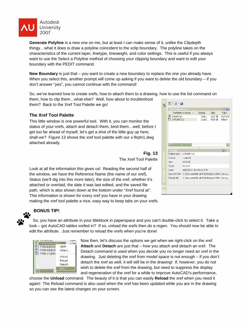
The Xref Tool Palette This little window is one powerful tool. With it, you can monitor the status of your xrefs, attach and detach them, bind them…well, before I get too far ahead of myself, let’s get a shot of the little guy up here, shall we? Figure 13 shows the xref tool palette with our x-flrpln1.dwg attached already.

Fig. 13 The Xref Tool Palette

Look at all the information this gives us! Reading the second half of the window, we have the Reference Name (the name of our xref), Status (we’ll dig into this more later), the size of the xref, whether it’s attached or overlaid, the date it was last edited, and the saved file path, which is also shown down at the bottom under “Xref found at”. This information is shown for every xref you have in your drawing making the xref tool palette a nice, easy way to keep tabs on your xrefs.

BONUS TIP!

So, you have an attribute in your titleblock in paperspace and you can’t double-click to select it. Take a look – got AutoCAD tables xrefed in? If so, unload the xrefs then do a regen. You should now be able to edit the attribute. Just remember to reload the xrefs when you’re done!

Now then, let’s discuss the options we get when we right-click on the xref. Attach and Detach are just that – how you attach and detach an xref. The Detach command is used when you decide you no longer need an xref in the drawing. Just deleting the xref from model space is not enough – if you don’t detach the xref as well, it will still be in the drawing! If, however, you do not wish to delete the xref from the drawing, but need to suppress the display and regeneration of the xref for a while to improve AutoCAD’s performance,

choose the Unload command. The beauty of it is that you can easily Reload the xref when you need it again! The Reload command is also used when the xref has been updated while you are in the drawing so you can see the latest changes on your screen.

Binding an Xref That’s right, folks, this is so important I’m giving it its own heading! When you bind an xref, you are making it and its dependent named objects (such as blocks, text styles, dimension styles, layers and linetypes) a part of the current drawing. The xref actually becomes inserted as a block in your drawing and loses all links to the xref drawing. Get those blank looks off of your faces, I’m going to explain that! Up until you hit the “bind” button, your xref in the drawing was linked to the xref file – it would be automatically updated when you changed the xref file. Once you bind the xref, however, it breaks that link. Instead of an xref, you now have a block inserted into your drawing that can be exploded, changed, etc. When is this helpful? When you’re sending someone else your drawing files. If an architect wants to see my latest plumbing drawings, I’ll bind the xrefs to the drawings so that I know he has them. How many of you have received drawings and had some, if not all, of the xrefs missing? This is how we can break the cycle of missing xrefs! Binding also is used when archiving a project – again, no missing xrefs this way! (Of course, the incredibly simple way to transmit drawings is to do an “etransmit” of them – that way all the xrefs, fonts, etc. are included in one easy package. Read up on it – it’s awesome!) Please note: after binding an xref, the layers associated with it will now show up differently in your Layer Manager, as shown in Figure 14 below.

Fig. 14 Bound Xref Layers in Layer Manager

Opening an Xref in the Drawing Ok, this is me getting down on my knees and begging you – be very, VERY careful with this command! It’s dangerous! Right-clicking when the xref is selected gives you two choices – “Edit in Place” and “Open Xref”. Edit in Place does just that – opens the xref in the drawing you’re in for editing. Be very, very careful when doing that – if your drawing crashes, you will lose BOTH drawings – the one you were in and your xref file. Go for Open Xref instead – that will open the xref in a new window and you can work on it there.

Xref Status I told you I’d be back to this one. If you look back at Figure 13, you’ll see that the current status of the floorplan.dwg is “loaded”, which simply means it’s in the drawing and life is good. However, there are other words that can show up in that column:

• Loaded: Currently attached to the drawing. • Unloaded: Marked to be unloaded from the drawing once the Xref Manager is closed. • Unreferenced: Attached to the drawing but erased. • Not Found: No longer exists in the valid search paths. • Unresolved: Cannot be read by AutoCAD. • Orphaned: Attached to another xref that is unreferenced, unresolved, or not found.

We’ve discussed “unloaded” before…simply hit “reload” and your xref is back. “Unreferenced” can only be fixed by reinserting the xref – once you’ve erased it, there’s no getting it back (unless you want to hit undo a lot). If the xref comes up “not found”, then chances are the xref has been moved from the folder you were keeping it in. This is where the “xref found at” bar comes in. Using the “browse” button next to it, you need to tell AutoCAD where it should now look for the xref. Make sure you hit “save path” after you’ve found it! Should you get the “unresolved” message, then your xref may need auditing or purging, or may be in a version you can’t read (you’re running 2006, it’s saved in 2007…not gonna work!). That leaves us with “orphaned”, which is now self-explanatory, right? Please say “right”.

Congratulations! You’re now all xref wizards! People will bow down before you, amazed at your skills…ok, probably not, but hopefully I’ve helped clear up any questions you’ve had about xrefs.

BONUS TIPS You can Trim and Extend to xref entities. Want that piping line to stop at that wall? No problem! When inserting an xref, once you’ve navigated to the folder the xref is kept in you can just type in the drawing name instead of scrolling through the list. All right, so now that we’ve talked xrefs for a while, let’s move on to hatching, shall we?

What is a Hatch? A hatch is a pattern that you fill an area with to differentiate components of a project or to signify the material composing an object. They can also be used for shading areas to mark project phases or to add detail to drawings. Depending on how you wish to use them, they can be anything from quick and easy to downright complex! This class will focus on the basics of creating and editing hatches. Now then, should any of you out there know oodles about creating your own hatch patterns; know that I will not be covering that topic here.

The Hatch Dialog Box To begin with, we need something to hatch. Draw up a simple 6’x8’ rectangle, then go ahead and select the Hatch command from the Draw menu, or just click on the Hatch button on the toolbar as shown in Figure 15. The Boundary Hatch and Fill dialog box will pop open. Take a good look at Figure 16 – this is where you define everything about your hatch.

Fig. 15 Hatch Command

Fig. 16 The Boundary Hatch and Fill Dialog Box

In case you hadn’t noticed, there are a lot of choices here! Let’s take this one step at a time.

Hatch Type and Pattern These two are as good place to begin as any. This is where you choose what your hatch is going to look like. If you hit the drop-down menu on “Type”, you’ll see three options: predefined, user defined, and custom. The differences are as follows:

Predefined These patterns are stored in the acad.pat and acadiso.pat files and are the ones that come preloaded in AutoCAD. You can control the angle and scale of any predefined pattern. For predefined ISO patterns, you can also control the ISO pen width. Note: When you use the Solid predefined pattern, the boundary must be closed and must not intersect itself.

User Defined Creates a pattern of lines based on the current linetype in your drawing. You can control the angle and spacing of the lines in your user-defined pattern.

Custom Specifies a pattern that is defined in any custom PAT file that you have added to the AutoCAD search path. (To use the patterns in the supplied acad.pat and acadiso.pat files, choose Predefined.) You can control the angle and scale of any custom pattern.

Hatch Angle and Scale “Angle” specifies an angle for the hatch pattern relative to the X-axis of the current UCS. “Scale” expands or contracts a predefined or custom pattern. This option is available only if you set “Type” to “Predefined” or “Custom”. How you wish to scale the pattern is totally dependent upon what you want the final product to look like. You’ll see how this works when we draw a hatch in a few moments. Note: if you draw a hatch in paper space, save yourself some grief and check the “Relative to Paper Space” box. Using this option, you can easily display hatch patterns at a scale that is appropriate for your layout.

Hatch Spacing and ISO Pen Width The “Spacing” option will only become available when you select a user-defined pattern. Again, we will not be discussing those in this lesson, but I figured you’d like to know what it was. If you were using a user-defined pattern, this would be where you specified the spacing of your lines. “ISO Pen Width” is only available when you set “Type” to “Predefined” and set “Pattern” to one of the available ISO patterns. It scales the ISO pattern based upon the selected pen width.

Hatch Origin By default, hatch patterns always “line up” with each other. However, sometimes you might need to move the starting point, called the origin point, of the hatch. For example, if you create a brick pattern, you might want to start with a complete brick in the lower-left corner of the hatched area. In that case, use the Hatch Origin options in the Hatch and Gradient dialog box.

Object Selection

Take a look at the side of the dialog box as I’ve highlighted in Figure 03. We have several different options here, including some that are grayed-out at the moment. Depending on what the area you’re trying to shade looks like, one of these will always be easier than the other. Let’s meet them, shall we?

Fig. 17 Hatch and Fill Dialog Box – Object Selection

Pick Points

This determines a boundary from existing objects visible on the screen. The objects must form an enclosed area. When you select Pick Points, the dialog box closes temporarily, and AutoCAD displays a prompt.

Select internal point: Specify a point within the area to be hatched or filled

Select internal point: Specify a point, enter u or undo to undo the last selection, or press ENTER to end point specification and return to the dialog box

While specifying points, you can right-click in the drawing area at any time to display a shortcut menu. You can undo the last or all point specifications, change the selection method, change the island detection style, or preview the hatch or gradient fill.

Select Objects This is the easiest, quickest way possible to select a hatch boundary. If you have a polyline drawn around your area or your area is a closed object (rectangle, circle, etc.) then this is the option for you! What it does is it determines a boundary from selected objects that form an enclosed area. The dialog box closes temporarily, and you are prompted to select objects:

Select objects or [picK internal point/remove Boundaries]:Select objects that define the area to be hatched or filled, specify an option, enter u or undo to undo the last selection, or press ENTER to return to the dialog box

Each time you click Select Objects, HATCH clears the previous selection set. While selecting objects, you can right-click at any time in the drawing area to display a shortcut menu. You can undo the last selection or all selections, change the selection method, change the island detection style, or preview the hatch or gradient fill.

Associative This is a neat little guy – you can choose to have the hatch update itself if you change the hatch boundary. By choosing “associative”, whenever you edit the hatch boundary the hatching will update itself automatically. If you deselect “associative”, then if you change the boundary you will have to recreate the hatch.

Create Separate Hatches Remember in the olden days of AutoCAD when if you tried to hatch several areas at once, you wound up with one big hatch? No more! You can select several different areas to hatch and with this little box checked, it will create several different hatches.

Draw Order Same as the main AutoCAD draw order command – it assigns the draw order to a hatch or fill. You can place a hatch or fill behind all other objects, in front of all other objects, behind the hatch boundary, or in front of the hatch boundary.

Inherit Properties This comes in handy if we had previously made a hatch and wanted to use the exact same one for another area. The command hatches or fills specified boundaries using the hatch or fill properties of a selected hatch object. When you click Inherit Properties, the dialog box closes temporarily, and the command line displays a prompt:

Select hatch object: Click within a hatched or filled area to select the hatch whose properties are to be used for the new hatch object

So, what if you now want to go back and change one of the hatches? This is where the Hatch Edit dialog box comes in!

Hatch Editing Ok, so you’ve been hatching like a fiend. Suppose you look over your drawing and decided that we want the hatch scale to be different. You could go through, erase the old hatch and make a new one, blah blah blah…but who wants to do that? Instead, you can just edit the existing hatch though the magic of the hatch editor!

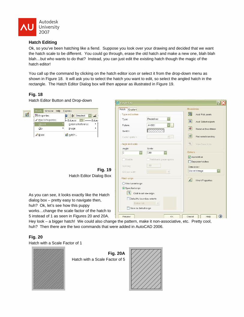
You call up the command by clicking on the hatch editor icon or select it from the drop-down menu as shown in Figure 18. It will ask you to select the hatch you want to edit, so select the angled hatch in the rectangle. The Hatch Editor Dialog box will then appear as illustrated in Figure 19.

Fig. 18 Hatch Editor Button and Drop-down

Fig. 19 Hatch Editor Dialog Box

As you can see, it looks exactly like the Hatch dialog box – pretty easy to navigate then, huh? Ok, let’s see how this puppy works…change the scale factor of the hatch to 5 instead of 1 as seen in Figures 20 and 20A. Hey look – a bigger hatch! We could also change the pattern, make it non-associative, etc. Pretty cool, huh? Then there are the two commands that were added in AutoCAD 2006.

Fig. 20 Hatch with a Scale Factor of 1

Fig. 20A Hatch with a Scale Factor of 5

Remove Boundaries

Say you wanted something you hatched previously to not be hatched anymore – bye bye hatch!

Recreate Boundaries

Ever have one of those days where you created a hatch and then erased the boundary lines? Here’s your new undo button – this will redraw the boundary lines used to create the hatch.

All right, now that we’re all hatching fools, let’s tackle our last subject – Raster Images!

What is a Raster Image? A raster image is an image file (.jpg, .bmp, etc.) that is attached to a drawing in much the same way an xref is. It can be clipped, rotated, scaled, moved, and cursed at frequently depending on what you’re trying to do with it! Those of you who’ve dealt with these little buggers before should be nodding your head and agreeing with me at this point. If you’ve never seen a raster image before, well, get ready for a love-hate relationship with the things.

Raster images are being used more and more these days. Companies use them to insert their logos in titleblocks, architects and interior designers will use them for providing better visuals to a client, engineering firms can use them to trace existing ductwork and pipe lines with and they’re used in presentation drawings to show photos of a site. They really are handy to have, but controlling them…that’s the interesting part.

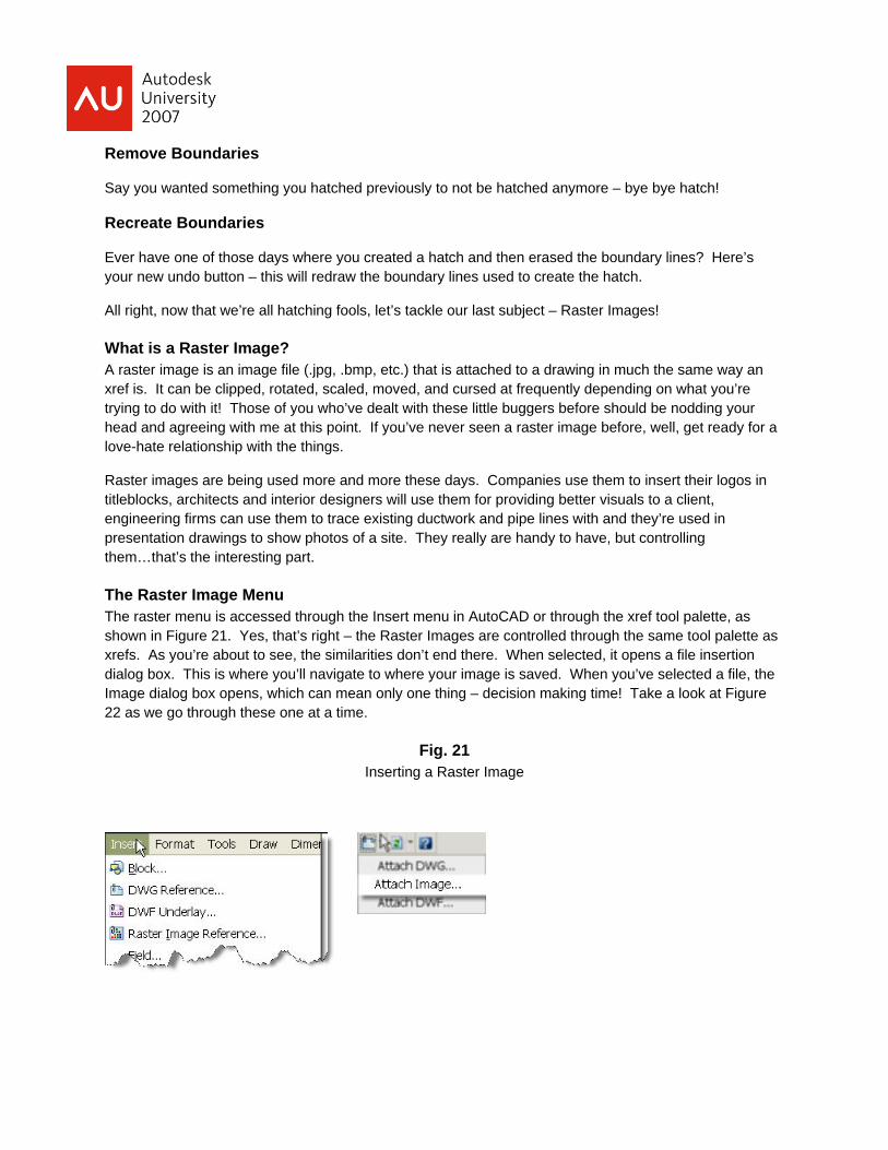
The Raster Image Menu The raster menu is accessed through the Insert menu in AutoCAD or through the xref tool palette, as shown in Figure 21. Yes, that’s right – the Raster Images are controlled through the same tool palette as xrefs. As you’re about to see, the similarities don’t end there. When selected, it opens a file insertion dialog box. This is where you’ll navigate to where your image is saved. When you’ve selected a file, the Image dialog box opens, which can mean only one thing – decision making time! Take a look at Figure 22 as we go through these one at a time.

Fig. 21 Inserting a Raster Image

Fig. 22 Raster Insertion Menu

Path Type Identical to the xref choices, you have three different options when it comes to path type – full path, relative path, and no path.

Full Path - Specifies the absolute path to the image file.

Relative Path - Specifies a relative path to the image file.

No Path - Specifies only the image file name. The image file should be located in the folder with the current drawing file.

Insertion Point As usual, this specifies where you want the image to wind up on your drawing. My favorite is still the “specify onscreen” option as I can make sure that it’s landing where I want it to. For those of you who aren’t quite the control freak I am, however, here’s the description of how to specify it before inserting it.

If Specify On-Screen is cleared, enter the insertion point in X, Y, and Z.

X - Sets the X coordinate value.

Y - Sets the Y coordinate value.

Z - Sets the Z coordinate value.

Scale Yup, you guessed – specifies the scale of the image. Isn’t it nice when these choices mean exactly what you think they mean? Specify On-Screen directs input to the command line or the pointing device. If Specify On-Screen is cleared, enter a value for the scale factor. The default scale factor is 1.

If INSUNITS is set to “unitless” or if the image does not contain resolution information, the scale factor becomes the image width in AutoCAD units. If INSUNITS has a value such as millimeters, centimeters, inches, or feet, and the image has resolution information, the scale factor is applied after the true width of the image in AutoCAD units is determined.

Rotation Ahh, rotation – the command that keeps us from having vertical pictures wind up horizontal. If Specify On-Screen is selected, you may wait until you exit the dialog box to rotate the object with your pointing device or enter a rotation angle value on the command line. If Specify On-Screen is cleared, enter the rotation angle value in the dialog box. The default rotation angle is 0.

Details Now here’s something new. All the choices so far mirror the xref attach choices as you’re essentially doing the same thing. Details, however, is unique to the raster image. It displays the Image Information section. You can view width and height in pixels, the resolution, and the size in units (such as millimeters, centimeters, meters, kilometers, inches, feet, yards, miles, unitless, and many others). The default value for unitless images is unitless. The image size is automatically converted to AutoCAD units and is displayed at the default width and height. You can see what all this looks like in Figure 23.

Resolution Displays information about the vertical and horizontal resolution of the selected image.

Current AutoCAD Unit Displays information about the default units of the selected image. The image is displayed at the default width and height in pixels.

Image Size in Pixels Displays information about the width and height in pixels of the selected image.

Image Size in Units Displays information about the default size in units of the selected image. The image size is automatically converted to AutoCAD units and is displayed at the default width and height.

Fig. 23 Raster Image Details

Manipulating Raster Images Ok, first rule – the only way to select a raster image is by its image frame. The image frame is a black box around the image. This is the piece of geometry you have to select – clicking on the center of the picture won’t do a thing! Take a look at Figure 24 – I’ve got the grips on for the frame to show you what I’m talking about.

Fig. 24 Raster Image Frame

Now then, another word about image frames – they will

usually print if you leave them on! This is why there’s a command called “imageframe”. Yes, I said “usually”. New to

2006 was a fabulous image frame system variable. Type in or select the command and your choices are 0, 1, or 2. The results are as follows:

0 – Image frames are not displayed and not plotted

1 – Image frames are both displayed and plotted

2 – Image frames are displayed but not plotted

Setting the variable to ‘2’ is a common choice – you can see the frame still to edit the raster image, but you don’t have to worry about turning it off like in the old days so that it doesn’t show up on the plot. It’s the best of both worlds!

Now that we know how to select our image, let’s see what we can do with it!

Details

Suppose you have the picture shown in Figure 25. I don’t want the whole image shown here, just a piece of it. Well, just like xrefs you can clip a raster image. The clipping boundary can be a rectangle or a two-dimensional (2D) polygon with vertices within the boundaries of the image. Each instance of an image can only have one clipped boundary. Multiple instances of the same image can have different boundaries. You can change the boundary of a clipped image.

Fig. 25 Raster Image in need of Clipping

You can display a clipped image using the clipping boundary, or you can hide the clipping boundary to display the image with its original boundaries, same as an xref. This way you can see what the full image was if you want to adjust the boundary. Also like the xref, you can

delete the clipping boundary and restore the full image. Figure 26 shows the final clipped image. Fairly simple, right?

Fig. 26 Raster Image after Clipping

Modifying the Image You can also change several display properties of raster images in a drawing for easier viewing or special effects. All of the commands are available off the Modify pull-downs or by selecting the image and right-clicking on the screen.

Image Adjust You can adjust brightness, contrast, and fade for the display of an image as well as for plotted output without affecting the original raster image file and without affecting other instances of the image in the drawing. Adjust brightness to darken or lighten an image. Adjust contrast to make poor-quality images easier to read. Adjust fade to make drawing geometry easier to see over images and to create a watermark effect in your plotted output. To do this, select Modify>Object>Image>Adjust and use the slider bars shown in Figure 27 to adjust your image, just like adjusting pictures from a digital camera. The image on the side is a preview window for the changes you’re making, so you know immediately how the final image will appear.

Fig. 27 Raster Image Adjust Menu

Image Display You have two setting choices here – high and draft. High quality images mean that they appear and print exactly like the original picture, but they slow down the drawing during loading, regens, etc. Draft

quality images appear more grainy (depending on the image file type), but they are displayed more quickly than high-quality images.

BONUS TIP

You can set the Image Display to Draft quality and not have to worry when it comes time to plot – AutoCAD always plots images using High quality.

Image Transparency Again, two choices – on or off. On means that the image is now transparent and objects can be seen beneath it. Off means, well, that you can’t. It’s nice when these commands aren’t really complicated, isn’t it?

And now, the catch… As you may have noticed (probably from my constantly saying so) you treat raster images much the same way that you treat xrefs. You can clip them, specify the paths, move them…but you cannot bind them. Yes folks, this is what the major problem is with image files. You have to keep them with the drawings when archiving them, sending them to other people (etransmit, anyone?), and have to be very careful not to move them out of the original directory. If you do move them, be sure to redefine the path in the Xref Manager Tool Palette, the same way you would for an xref.

All right, thank you all for attending and have a safe trip home! All you AUGI members; see you in the forums!