xx predictability for timing and temperature in

XX

Predictability for Timing and Temperature in MultiprocessorSystem-on-Chip Platforms

LOTHAR THIELE, LARS SCHOR, IULIANA BACIVAROV,and HOESEOK YANG, ETH Zurich

High computational performance in multiprocessor system-on-chips (MPSoCs) is constrained by the ever-increasing power densities in integrated circuits, so that nowadays MPSoCs face various thermal issues.For instance, high chip temperatures may lead to long-term reliability concerns and short-term functionalerrors. Therefore, the new challenge in designing embedded real-time MPSoCs is to guarantee the final per-formance and correct function of the system, considering both functional and non-functional properties. Oneway to achieve this is by ruling out mapping alternatives that do not fulfill requirements on performance orpeak temperature already in early design stages. In this article, we propose a thermal-aware optimizationframework for mapping real-time applications onto MPSoC platforms. The performance and temperatureof mapping candidates are evaluated by formal temporal and thermal analysis models. To this end, analy-sis models are automatically generated during design space exploration, based on the same specificationsas used for software synthesis. The analysis models are automatically calibrated with performance datareflecting the execution of the system on the target platform. The data is automatically obtained prior to de-sign space exploration based on a set of benchmark mappings. Case studies show that the performance andtemperature requirements are often conflicting goals and optimizing them together leads to major benefitsin terms of a guaranteed and predictable high performance.

Categories and Subject Descriptors: C.3 [Special-Purpose and Application-Based Systems]: Realtimeand embedded systems; C.4 [Performance of systems]: Measurement techniques

General Terms: Design, Performance, Reliability

Additional Key Words and Phrases: MPSoC, temperature analysis, design automation

ACM Reference Format:Thiele, L., Schor, L., Bacivarov, I., and Yang, H. 2012. Predictability for timing and temperature in multipro-cessor system-on-chip platforms. ACM Trans. Embedd. Comput. Syst. XX, XX, Article XX ( 2012), 25 pages.DOI = 10.1145/0000000.0000000 http://doi.acm.org/10.1145/0000000.0000000

1. INTRODUCTIONMultiprocessor system-on-chips (MPSoCs) are a promising solution to keep pace withthe ever-increasing demand of computational performance. But as the obtained per-formance imposes a major rise in power consumption per unit area, MPSoCs can havea high chip temperature problem. Nowadays, the thermal wall is recognized as oneof the most significant barriers towards high performance systems [Hardavellas et al.2011]. For example, high chip temperatures may lead to long-term reliability concernsand short-term functional errors. Therefore, providing guarantees on maximum tem-perature is as important as functional correctness and timeliness when designing em-

This research has been founded by EU FP7 projects EURETILE and PRO3D, under grant numbers 247846and 249776.Author’s addresses: L. Thiele, L. Schor, I. Bacivarov, and H. Yang, Computer Engineering and NetworksLaboratory, ETH Zurich, CH-8092 Zurich, Switzerland; email: [email protected] to make digital or hard copies of part or all of this work for personal or classroom use is grantedwithout fee provided that copies are not made or distributed for profit or commercial advantage and thatcopies show this notice on the first page or initial screen of a display along with the full citation. Copyrightsfor components of this work owned by others than ACM must be honored. Abstracting with credit is per-mitted. To copy otherwise, to republish, to post on servers, to redistribute to lists, or to use any componentof this work in other works requires prior specific permission and/or a fee. Permissions may be requestedfrom Publications Dept., ACM, Inc., 2 Penn Plaza, Suite 701, New York, NY 10121-0701 USA, fax +1 (212)869-0481, or [email protected]© 2012 ACM 1539-9087/2012/-ARTXX $10.00

DOI 10.1145/0000000.0000000 http://doi.acm.org/10.1145/0000000.0000000

ACM Transactions on Embedded Computing Systems, Vol. XX, No. XX, Article XX, Publication date: 2012.

XX:2 L. Thiele et al.

bedded real-time MPSoCs. Aware of performance-temperature dependency, we takethe new challenge of optimizing the system design with respect to both performanceand temperature. More specifically, we aim at ruling out mapping alternatives thatdo not conform to real-time and peak temperature requirements already in early de-sign stages. Optimizing a system in both respects leads to major benefits in terms of aguaranteed and predictable high performance.

In this article, we present a high-level optimization framework for mapping real-time applications onto embedded MPSoC platforms that provides guarantees on bothtemporal and thermal correctness. The timing and temperatures of mapping candi-dates are evaluated by means of formal worst-case real-time analysis methods to pro-vide safe bounds on the execution time and the maximum chip temperature. Prac-tically, we extend the distributed operation layer (DOL) [Thiele et al. 2007; Huanget al. 2012] with the ability to perform not only performance analysis, that is done inmodular performance analysis (MPA) [Wandeler et al. 2006], but also to relate it tohigh-level temperature analysis in design space exploration.

The method proposed in [Schor et al. 2012] to analyze the worst-case chip temper-ature of an MPSoC platform is implemented as an extension of MPA so that bothtemperature and real-time analysis are done within the same framework in order tospeed up design space exploration. Furthermore, to explore the design space withoutuser-interactions, the analysis models are automatically generated from the same setof specifications as used for software synthesis. To increase the model accuracy, theanalysis models are calibrated with data corresponding to the target platform. Thedata is obtained in an automatic manner by either simulation on a virtual platform orexecution on the real hardware, prior to design space exploration.

Based on a prototype implementation of the proposed high-level mapping optimiza-tion framework, we demonstrate that there is no single optimal solution with respectto both real-time system performance and temperature, but all generated solutionsare worst-case guaranteed with respect to application behavior and impact of a non-deterministic environment. With the proposed framework, designers receive a pow-erful tool to map applications onto MPSoC platforms so that the system can safelyexecute without further involving other (dynamic) thermal management strategies,which may lead to unpredictable behavior. The contributions of this paper can be sum-marized as follows:

— A systematic approach to integrate worst-case real-time and peak temperature anal-ysis methods into a unique framework for MPSoC platforms is developed.

— To guarantee the accuracy of system analysis, we show that the proposed timingand thermal analysis models can be generated from the same set of specificationsas used for software synthesis without user-interaction and automatically calibratedwith performance data corresponding to the target platform.

— The viability of the proposed approach is demonstrated by the integration into ahigh-level optimization framework for mapping real-time applications onto embed-ded MPSoC platforms, namely DOL. Finally, the framework is applied to realisticcase studies to provide guarantees on temporal and thermal correctness of the sys-tem, and make timing and temperature aware decisions.

The remainder of the article is organized as follows: First, related work is discussedin the next section. Afterwards, Section 3 presents the mapping optimization frame-work including the fully automated design flow. Section 4 introduces the computationaland thermal models used for formal system analysis. The thermal analysis method isdescribed in Section 5. The automated generation and calibration of the thermal anal-ysis model is presented in Section 6 and finally, Section 7 presents case studies tohighlight the viability of our methods.


Predictability for Timing and Temperature in Multiprocessor System-on-Chip Platforms XX:3

2. RELATED WORKBy providing automatic mapping of applications onto distributed platforms, model-based frameworks outperform heuristic-driven approaches in terms of efficiency andprofit for the design of embedded multiprocessor systems [Zhao et al. 2005]. Examplesof model-based frameworks are Artemis [Pimentel 2008], Koski [Kangas et al. 2006],or DOL [Thiele et al. 2007; Huang et al. 2012]. In order to predict timing behavior ofembedded systems, all model-based frameworks include performance analysis of un-derlying multiprocessor systems. Often, analysis methods are classified based on theirscope [Bacivarov et al. 2010]. For example, performance analysis can be based on sim-ulation at different levels of abstractions or worst-case/best-case analysis. Simulation-based methods suffer various drawbacks over worst-case/best-case models as for ex-ample long run times and insufficient coverage of corner cases. Examples of best-case/worst-case analysis methods for multiprocessor systems are MPA [Wandeler et al.2006] or SymTA/S [Henia et al. 2005] that provide upper and lower bounds on timingproperties.

Thermal constraints are considered as the most significant barrier towards highperformance in modern MPSoC platforms [Hardavellas et al. 2011]. Increased powerdensities induce hot spot heat fluxes leading to high chip-temperatures, which in turncause long-term reliability concerns and short-term functional errors [Coskun et al.2007]. Reduced on-chip wire length motivates the use of three-dimensional stackingin the future [Loh 2008], which even magnifies problems with temperature [Zhu et al.2008]. Consequently, modern mapping optimization frameworks for real-time systemshave to consider both timing metrics and the thermal characteristics of the systemdesign. However, none of the above-mentioned model-based frameworks includes tem-perature analysis.

Nowadays, to address thermal issues, reactive thermal management tech-niques [Donald and Martonosi 2006; Brooks and Martonosi 2001; Kumar et al. 2006]are typically used. For example, multiple architectural-level techniques for ther-mal management like DVFS and stop-go scheduling are evaluated in [Donald andMartonosi 2006]. Causing a significant degradation of performance or leading to ex-pensive run-time overhead, reactive thermal management techniques are often unde-sirable in today’s embedded systems, in particular when tackling real-time constraints.On top of that, reactive thermal management techniques become more and more un-feasible as the operating voltage is limited by saturation [Watanabe et al. 2010]. Thealternative is to adopt system-level mechanisms, and already include temperatureanalysis at design-time.

Thermal aware task allocation and scheduling algorithms for MPSoC platforms areexplored in [Xie and Hung 2006; Coskun et al. 2007; Chantem et al. 2008]. In par-ticular, thermal aware heuristics to reduce the maximum and average temperatureare compared with power aware heuristics in [Xie and Hung 2006]. Thermal manage-ment techniques with unknown workload like load balancing or temperature awarerandom scheduling are discussed in [Coskun et al. 2007]. A mixed-integer linear pro-gramming formulation to reduce the peak temperature of an application is proposedin [Chantem et al. 2008]. All these design-time methods have in common that the tem-perature analysis is performed by either simulation or steady-state analysis. First,the transient power dissipation of the system is determined by means of a (poweraware) simulator, either software-based [Bartolini et al. 2010; Thiele et al. 2011] orhardware-based [Garcia del Valle and Atienza 2010]. Afterwards, power dissipationis used to calculate either the average temperature based on a steady-state analy-sis [Yang et al. 2010] or to evaluate the transient temperature evolution in a thermalsimulator. HotSpot [Huang et al. 2006; Skadron et al. 2004] and 3D-ICE [Sridhar et al.



2010] are the most common examples of such thermal simulators. However, due to thecomplexity of today’s systems, it is difficult to identify corner cases that actually lead tothe maximum temperature of the system under all feasible scenarios of task arrivals.Consequently, simulation-based thermal analysis methods may lead to an undesiredunderestimation of the maximum temperature.

Instead of simulation, we use formal thermal analysis methods to predict the worst-case temperature. [Rai et al. 2011] proposed a method to calculate the worst-case peaktemperature of a single-node system with non-deterministic workload. By incorporat-ing the heat transfer among neighboring nodes, [Schor et al. 2012] proposed a methodto calculate the worst-case chip temperature of an MPSoC platform. The article athand extends this work by proposing a systematic approach to integrate worst-casechip temperature analysis into a model-based framework. Moreover, joint effects ofperformance and temperature have not been considered so far in any model-basedframework for designing multiprocessor systems. By including timing and thermalanalysis into the same framework, we provide to system designers a powerful decisiontool, which includes both real-time and peak temperature analysis.

3. MAPPING OPTIMIZATION FRAMEWORKTo optimize the mapping of a streaming application onto an MPSoC platform withrespect to both worst-case performance and worst-case chip temperature, we extendDOL [Thiele et al. 2007] that has already successfully been applied to many architec-tures like MPARM platform [Benini et al. 2005], Sony/Toshiba/IBM Cell BE [Kahleet al. 2005], or Atmel DIOPSIS 940 [Paolucci et al. 2006]. Following the Y-chartparadigm [Kienhuis et al. 1997], the application and architecture are specified sepa-rately, and then linked by a mapping. This separation of concerns enables the iterativeimprovement of the system by modifying either of these specifications. The rest of thissection discusses first the application, architecture, and mapping models, and then,it introduces the design flow considered in this paper. In order to illustrate the usednotation, an example system is illustrated in Fig. 1a.

3.1. Application ModelIn the scope of this article, the synchronous data flow (SDF) [Lee and Messerschmitt1987] model of computation is considered in order to specify the application behaviorindependently of the communication. More formally, we represent an SDF applicationas a directed, connected graph A = (V,Q,W ) where every process v ∈ V represents anode in the graph. Edges model unbounded channels q ∈ Q, which in turn are used byprocesses to communicate with each other. W = {w1, . . . , w|Q|} describes the token con-sumption behavior of channels. The token consumption wq of channel q is representedas a triple (pq, cq, dq). Assuming q connects nodes v1 and v2, the number of tokens pro-duced by node v1 in every execution is denoted pq; cq is the number of tokens consumedin every execution by v2; and the initial amount of tokens in channel q is dq.

In the SDF model of computation, tasks represent processes that execute concur-rently. If they are mapped onto different processing elements, they can execute inparallel. Data dependencies are taken into account by means of edges that explicitlymodel the data flow between processes. A task is blocked as long as not all its prede-cessor tasks have produced the number of tokens the task needs to be triggered, thatis, there is at least one incoming channels q, which contains less than cq tokens. Oncetriggered, the task can process the received tokens independently of all other tasks andpredecessor tasks can simultaneously start to process the next tokens. The separationof computation and communication has various advantages with respect to softwaredevelopment. In particular, for system analysis, this separation enables the modular



v1

v3

v2

v4

bus

c1 c2

b1 = 1

b3 = 1b2 = 2 b4 = 2

pq1

pq2

pq3

pq4

cq1

cq2

cq3

cq4

q1

q2

q3

q4

(a) Formal system specification.

v1ain

v3

v2

v4

b2

c1 c2

bus1

bus2

TDMA

b1 bslot1 bslot2

bus

FP FP

(b) MPA model.

Fig. 1. System specification and the corresponding MPA model.

generation and calibration of analysis models from the same specification as it is usedfor actual system synthesis.

As we will see in Section 4, the analysis model is based on MPA that abstracts theworkload in any time interval ∆ ≥ 0 by a so-called arrival curve. Therefore, the resultsof this paper hold for other model of computations, as well. In particular, the onlyrequirement for the model of computation is that the workload of every independentcomponent is bounded in any time interval ∆ ≥ 0.

3.2. Architecture ModelUnlike temporal analysis, thermal analysis requires a detailed description of thearchitecture to model the heat flow between neighboring nodes. The architectureT = {χ1, . . . , χn} is assumed to be a heterogeneous multiprocessor system with n pro-cessing components connected by a shared bus or a network-on-chip. The placement ofcomponents is specified by a floorplan, see [Atienza et al. 2007] for examples of MPSoCfloorplans.

3.3. Mapping ModelThe mapping specification describes both the binding b of processes to architecturecomponents and their scheduling σ on shared resources. The binding can be repre-sented by a vector b = (b1; . . . ; b|V |) ∈ {1, . . . , n}|V | where bi = k if process vi is assignedto processing component χk. The scheduling policy is supposed to be work-conserving,that is, the processing component has to process as soon as there is data available. Thisassumption applies to most traditional scheduling algorithms as for example, earliest-deadline-first (EDF), rate-monotonic (RM), fixed-priority (FP), and deadline-monotonic(DM). For simplicity, we neglect the mapping of communication channels, and implic-itly assume that they are mapped onto the same processing component as the senderprocess, e.g. local memory of the corresponding processor, even though our tool can dealwith cases that are more general. The extension to mapping communication channelsis obvious in general and only augments the dimensionality of the design space.

3.4. Design FlowSo far, we discussed the specification of the application, architecture, and mappingmodels, which form together the systems specification, that is, the input to softwaresynthesis. While the application and architecture specifications are provided by thesystem designer, the mapping is automatically calculated during the design flow. Next,we describe the steps to explore the optimal mapping, that is, the binding and schedul-ing of a multi-processor streaming application onto an MPSoC platform in a time andthermal optimal manner. By varying the binding of application elements, that is, pro-



model calibration

design space exploration(mapping optimization)

formal thermal / timing analysis

application specification A

architecture specification T

optimal mapping

(b*, σ*)

model

parameters

benchmark

mapping

candidate

mapping (b, σ)model generation

model evaluationthermal / timing

metrics

software

synthesis

execution on

hardware

simulation on

virtual Platform

Fig. 2. Design flow for mapping optimization.

cesses v ∈ V and channels c ∈ C, to computation and communication resources, aimedsystem properties are optimized. Figure 2 illustrates the design flow for mapping opti-mization as it is considered in this paper.

The design flow is composed of three major parts, namely model calibration, designspace exploration, and thermal and timing analysis. During design space exploration,the thermal and timing characteristics of every candidate mapping (b, σ) are analyzed.The corresponding analysis models are parameterized with precalculated model pa-rameters that are extracted during model calibration. The output of the considereddesign flow is the optimal mapping (b∗, σ∗) of the given multiprocessor application Aonto the MPSoC architecture T .

The acquisition of the required model parameters is denoted as model calibrationand is detailed in Section 6.2. Model calibration is performed based on a set of bench-mark mappings prior to analyzing the candidate mappings during design space ex-ploration. First, a benchmark implementation is generated by synthesizing the bench-mark system composed of the application, architecture, and benchmark mapping spec-ification. Then, the benchmark implementation is simulated on a virtual platform orexecuted on the real hardware. The required parameters are automatically extractedand stored in a database for later use during thermal and timing analysis.

Once the model parameters are extracted, the design space exploration tool can startto explore for optimal mappings by analyzing the performance and chip temperatureof various candidate mappings (b, σ). The proposed design flow bases the performanceanalysis on formal worst-case real-time analysis methods. In particular, modular per-formance analysis (MPA) [Wandeler et al. 2006; Huang et al. 2012] is used. In order toevaluate the performance of a single candidate mapping, the proposed mapping opti-mization framework first generates an abstract model out of the same set of specifica-tions as used for software synthesis, namely application, architecture, and candidatemapping specification. Then, in a second step, the abstract model is examined withrespect to timing and thermal characteristics. In particular, timing properties are an-alyzed by the methods described in [Huang et al. 2012] and the thermal properties bythe methods proposed in Section 5. We argue in this article that the considered designflow can be completely automated. In other words, after specifying the input, that is,the application and the architecture, the design flow calculates a good mapping (b∗, σ∗)without user interaction.



pℓ

dℓ

time interval Δ [ms]

αℓ(Δ) com

p.

dem

and [

ms]

0

jℓ

pℓ

(a) Arrival curve α` for PJD model.time interval Δ [ms]

com

p. dem

and /

acc.

com

p. ti

me

[ms] bℓ Δℓ

I Δℓ

A

αℓ(Δ) γℓ(Δ)

(b) Accumulated computing time function.

Fig. 3. Computational model.

The focus of this paper is on formal analysis methods, and their automated genera-tion and calibration. Thus, we do not detail the part on how to calculate good candidatemappings, but refer to the summary given in Section 2.

4. SYSTEM MODEL FOR WORST-CASE TIMING AND TEMPERATURE ANALYSISThis section introduces the formal models to analyze a streaming application on anMPSoC platform with respect to both timing and temperature.

Notation: Bold characters are used for vectors and matrices and non-bold charactersfor scalars. For example, H denotes a matrix whose (k, `)-th element is denoted Hk`

and T denotes a vector whose k-th element is denoted Tk.

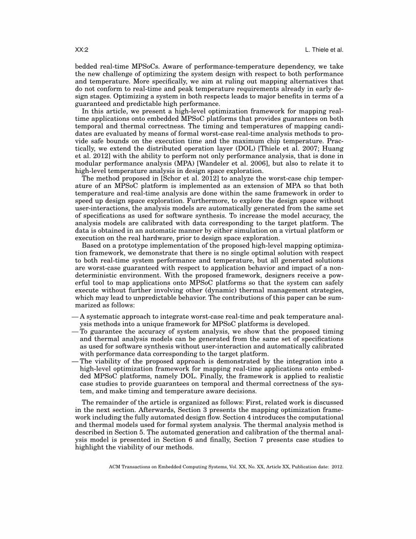
4.1. Computational ModelThe computational model for timing and thermal analysis is based on MPA [Wan-deler et al. 2006] that uses a compositional approach to split up a system into actorswith small interference. After separately characterizing each actor, the system is an-alyzed with real-time calculus [Thiele et al. 2000], which is based on network calcu-lus [Le Boudec and Thiran 2001]. Formally, we use a graph M = (V, E) to representan MPA model. The set of nodes V represents the actors and the set of edges E repre-sents event streams (abstracted by arrival curves α) and resource streams (abstractedby service curves β). The data dependency between different actors is given by theexecution sequence. Communication resources are described by the same concept ascomputational resources, namely by a cumulative function that defines the number ofavailable resources in any time interval. Figure 1b shows the MPA model of the mul-tiprocessor system from Fig. 1a. For illustration, we suppose fixed priority preemptivescheduling on all processors and TDMA scheduling on the bus even though other poli-cies can be modeled, as well. αin abstracts the system’s input stream, β1 and β2 abstractthe available resources of component χ1 and χ2. βslot1 and βslot2 abstract the resourceavailability of the bus. In the following, we will summarize the event stream and work-load models relevant to calculate the worst-case chip temperature of a multiprocessorsystem.

The considered model of an event stream follows the ideas of real-time calculus. Wesuppose that in time interval [s, t), events with a total workload of R`(s, t) time unitsarrive at component `. Each event is supposed to have a constant workload of ∆A

` timeunits. The arrival curve α` upper bounds all possible cumulative workloads:

R`(s, t) ≤ α`(t− s) ∀s < t (1)

with α`(0) = 0. For the scope of this article, we assume that an event stream can bespecified by a period p`, a jitter j`, and a minimum interarrival distance d` [Henia et al.2005], see Fig. 3a for a typical arrival curve.



We suppose that processing components are work-conserving. In other words, theywill be in ‘active’ mode as long as there are events in their ready queues. The re-source availability of such a component ` is abstracted by the service curve β`(∆) = ∆for all intervals of length ∆ ≥ 0. The accumulated computing time Q`(s, t) de-scribes the amount of time units that component ` is spending to process an incom-ing workload of R`(s, t) time units. Therefore, for work-conserving scheduling algo-rithms, the accumulated computing time Q`(s, t) in time interval [s, t) is Q`(s, t) =infs≤u≤t {(t− u) +R`(s, u)} provided that there is no buffered workload in the readyqueue at time s [Thiele et al. 2000]. Using arrival curve α`, the accumulated comput-ing time Q`(t−∆, t) can be upper bounded by γ`(∆) for all intervals of length ∆ < t:

Q`(t−∆, t) ≤ γ`(∆) = inf0≤λ≤∆

{(∆− λ) + α`(λ)} . (2)

For any fixed s with s < t, the accumulated computing time Q`(s, t) is monotonicallyincreasing and has either slope 1 or 0. Whenever the slope is 1, the component is in‘active’ processing mode, that is, it is processing events. When the slope is 0, the com-ponent is ‘idle’, that is, it is in sleep mode. The processing mode can be expressed bythe mode function:

S`(t) =dQ`(s, t)

dt=

{1 component ` is ‘active’,0 component ` is ‘idle’.

(3)

A typical arrival curve and its corresponding upper bound on the accumulated com-puting time function are outlined in Fig. 3b. We characterize the upper bound on thecomputing time of component ` by the length b` of the first interval with slope 1, alsocalled burst, the length ∆A

` of every other interval with slope 1, and the length ∆I` of

every interval with slope 0. While b` and ∆A` are constant for the considered compu-

tational model, we also assume for computational simplicity, that the upper bound onthe accumulated computing time is selected so that all intervals with slope 0 have thesame length.

4.2. Thermal ModelA well-accepted thermal model of an MPSoC architecture with |T | processing com-ponents is to describe the temperature evolution by means of an equivalent RC cir-cuit [Krum 2000; Skadron et al. 2004; Huang et al. 2006; Chantem et al. 2008]. The ver-tical layout of the chip is modeled by four layers, namely the heat sink, heat spreader,thermal interface, and silicon die. Each layer is divided into a set of blocks accordingto architecture-level units, that is, in our case, processing components. Figure 4 rep-resents an example floorplan and its equivalent RC circuit of the silicon layer. Everyblock is then mapped onto a node of the thermal circuit. The number of nodes andtherefore, the order of the thermal model is n = 4 · |T |. In particular, the n-dimensionaltemperature vector T(t) at time t is described by a set of first-order differential equa-tions:

C · dT(t)

dt=(P(t) + K ·Tamb

)− (G + K) ·T(t) (4)

where C is the thermal capacitance matrix, G the thermal conductance matrix, K thethermal ground conductance matrix, P the power dissipation vector, and Tamb = T amb ·[1, . . . , 1]′ the ambient temperature vector. The initial temperature vector is denoted asT0 and the system is assumed to start at time t0 = 0. C, G, and K are calculated fromthe floorplan and thermal configuration of the chip. G is a non-positive matrix whosediagonal elements are zero and K is a non-negative diagonal matrix.



Component 1 Component 2

hei

gh

t 1

hei

gh

t 2

width1 width2

(a) Floorplan of an MPSoC platform with two pro-cessing components.

T1G12 = G21

K22K11 C22C11

T2

P1 P2

(b) Equivalent RC circuit of one layer of the MP-SoC platform in Fig. 4a.

Fig. 4. Floorplan and equivalent RC circuit.

We assume a linear dependency of power dissipation on temperature [Liu et al. 2007;Chantem et al. 2008] due to leakage power:

P(t) = φ ·T(t) +ψ(t) (5)

where φ is a diagonal matrix with constant coefficients, and ψ a vector with constantcoefficients. As we suppose that the leakage power of a component is independent ofits processing mode, we characterize the power dissipated by component ` in ‘active’and ‘idle’ processing mode as:

P`(t) =

{P a` (t) = φ`` · T` + ψa` if S`(t) = 1,

P i` (t) = φ`` · T` + ψi` if S`(t) = 0.(6)

Rewriting Eq. (4) with Eq. (5) leads to the state-space representation of the thermalmodel:

dT(t)

dt= A ·T(t) + B · u(t) (7)

where u(t) = ψ(t) + K ·Tamb is called the input vector, A = −C−1 · (G + K− φ), andB = C−1. As A and B are time-invariant, the considered thermal model represents alinear and time-invariant (LTI) system [Friedland 1986] and consequently for t > 0, aclosed-form solution of the temperature yields:

T(t) = eA·t ·T0 +

∫ ∞−∞

H(t− ξ) · u(ξ) dξ (8)

where H(t) = eA·t ·B. Hk`(t) corresponds to the impulse response between node ` andnode k. With Tinit(t) = eA·t ·T0, the temperature Tk(t) of node k is of form:

Tk(t) = T initk (t) +

n∑`=1

Tk,`(t) (9)

where Tk,`(t) is the convolution between the impulse response Hk` and the input u`:

Tk,`(t) =

∫ t

0

Hk`(t− ξ) · u`(ξ) dξ. (10)

By using the processing mode of component `, we can associate the input u` of node `with the workload of the corresponding component:

u`(t) = S`(t) · ua` + (1− S`(t)) · ui`. (11)

where ua` = ψa` +K`` · T amb and ui` = ψi` +K`` · T amb.As the impulse response describes the reaction of the system over time, next, we will

discuss its properties with respect to the considered thermal model. First, we note that



0 1 2 3 4 50

2.5

5

7.5

time t

Hkk(t)

(a) Self-impulse response Hkk(t).

0 1 2 3 4 50

0.5

1

1.5

tHkℓ

max

time t

Hkℓ(t)

(b) General impulse response Hk`(t).

Fig. 5. Impulse responses.

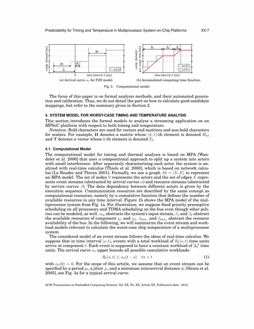
H(t) ≥ 0 for all t ≥ 0, as A is essentially non-negative, that is, Ak` ≥ 0 for all ` 6= k,which in turn leads to eA·t ≥ 0 [Birkhoff and Varga 1958]. The self-impulse responseHkk(t) can be calculated by Hkk(t) = e′k · eA·t · ek ·Bkk, where ek is the unit vector point-ing in k direction. Therefore, Hkk(0) ≥ Hkk(t) ≥ 0 for all t ≥ 0 and dHkk(t)

dt ≤ 0 [Maedaet al. 1977], see Fig. 5a for an illustration. Next, based on various experiments andthe self-impulse response, we conjecture that the general impulse response Hk`(t) is anon-negative unimodal function that has its maximum at time tHkj

max, that is, dHk`(t)dt ≥ 0

for all 0 ≤ t ≤ tHkjmax and dHk`(t)

dt ≤ 0 for all t > tHkjmax as illustrated in Fig. 5b. Intuitively,

this can be motivated by the duality of a thermal network and a grounded capacitorRC circuit. We know from [Gupta et al. 1997] that all impulse responses of a stable RCtree network are unimodal. As a particular path of a general RC network usually dom-inates the impulse response, we can neglect local maximums that are caused by differ-ent paths without significantly affecting the resulting temperature. In all performedexperiments, we never detected a departure from this conjecture. With temperaturein mind, this describes that temperature rises with power on the component that pro-duces power without a delay and on a neighbor of the component that produces poweronly after a delay.

5. TEMPERATURE ANALYSISThe framework presented in this article uses formal thermal analysis to calculate theworst-case chip temperature, that is, the maximum temperature of a chip under allfeasible scenarios of task arrivals. In this section, the thermal analysis method to cal-culate the worst-case chip temperature is described. We refer the reader to [Schor et al.2012] for detailed proofs of the theorems stated in this section.

Clearly, the worst-case chip temperature T ∗S of an MPSoC platform is the maximumtemperature of all individual nodes:

T ∗S = max (T ∗1 , . . . , T∗n) (12)

where T ∗k is the worst-case peak temperature of node k and n the number of nodes.We call the set of cumulative workload traces R that leads to the worst-case peaktemperature T ∗k of node k the critical set of cumulative workload traces and denote itwith R{k}. Because temperature rises with power consumed at another node only aftera delay and the delay is different for every two nodes, there is a different critical set ofworkload traces R{k} for every node k.

In the following, we present a constructive method to calculate R{k}. We start withcalculating the critical accumulated computing time Q{k} leading to T ∗k . Afterwards,we show that R{k}` (0, t) = ∆A

` ·⌈

1∆A

`

Q{k}` (0, t)

⌉is a valid workload and R{k}(0, t) =[

R{k}1 (0, t), . . . , R

{k}n (0, t)

]′actually results in the critical accumulated computing time

Q{k}. Finally, the worst-case peak temperature T ∗k (τ) of node k at observation time τis obtained by simulating the system with workload R{k}(0, t) for all t ∈ [0, τ).



5.1. Critical Accumulated Computing TimeIn this section, we construct the accumulated computing time Q{k} that maximizes thetemperature Tk(τ) at a certain observation time τ > 0. In a first step, we show thateach T ∗k,`(τ) defined by Eq. (10) can individually be maximized.

LEMMA 5.1 (SUPERPOSITION). Suppose that T ∗k,`(τ) = maxu`∈U`(Tk,`(τ)) with U`

the set of all possible inputs u`. Then, the worst-case peak temperature of node k attime τ is:

T ∗k (τ) ≤ T initk +

n∑`=1

T ∗k,`(τ) (13)

where n is equal the number of nodes of the thermal RC circuit. Equality is obtained ifthe workload of all processing components is independent of each other.

Lemma 5.1 indicates that each Tk,`(τ), at a certain time instance τ > 0, can individ-ually be maximized. As T ∗k,` only depends on Q

{k}` and Q

{k}` only affects T ∗k,`, we can

individually calculate every Q{k}` so that Q{k}` maximizes Tk,`(τ) at time instance τ .In the following, we introduce a method to construct the critical accumulated com-

puting time Q{k}` for each individual component `. Suppose that tHkjmax denotes the time

where Hk`(t) is maximum. First, we will show that a higher temperature is obtained attime instance τ if the processing component is in ‘active’ processing mode for a longeraccumulated computing time in any interval starting or ending at t̃Hkj

max = τ − tHkjmax. For

readability, we will show this statement only for t < t̃Hkjmax and refer to [Schor et al.

2012] for t > t̃Hkjmax. Lemma 5.2 shows that two mode functions defined by Eq. (3) that

are almost everytime the same, except in a small interval, result in different tempera-tures.

LEMMA 5.2 (SHIFTING). For any given time instance τ , we consider two mode func-tions S`(t) and S`(t) defined by Eq. (3) for t ∈ [0, τ). For given δ > 0, σ ≥ 0, σ+2δ < t̃

Hkjmax,

the two mode functions only differ as follows:

— S`(t) = 1 for all t ∈ [σ, σ + δ) (‘active mode’),— S`(t) = 0 for all t ∈ [σ + δ, σ + 2δ) (‘idle mode’), and— S`(t) = 1− S`(t) for all t ∈ [σ, σ + 2δ).

In other words, both mode functions have the same sequence of ‘active’ and ‘idle’ modesfor t ∈ [0, σ) and t ∈ [σ+ 2δ, τ). Then T k,`(τ) at time τ for mode function S`(t) is not lessthan Tk,`(τ) at time τ for mode function S`(t), that is, T k,`(τ) ≥ Tk,`(τ).

Based on Lemma 5.2, we show now that a higher temperature at time τ is obtained ifin any interval ending at t̃Hkj

max, the processing component is in ‘active’ processing modefor a longer accumulated time.

LEMMA 5.3 (MODE FUNCTIONS COMPARISON). For any given time instance τ , weconsider two accumulated computing time functions Q`, resulting from mode functionS`, and Q`, resulting from mode function S`, with:

Q`(t̃Hkjmax −∆, t̃

Hkjmax) ≥ Q`(t̃

Hkjmax −∆, t̃

Hkjmax) (14)

for all 0 ≤ ∆ ≤ t̃Hkjmax and S`(t) = S`(t) for all t̃Hkj

max < t ≤ τ . Then, T k,`(τ) at time τ formode function S`(t) is not less than Tk,`(τ) at time τ for mode function S`(t).



ALGORITHM 1: Calculation of the critical accumulated computing time function Q{k}` (0,∆)

for all 0 ≤ ∆ ≤ τ .

Input: b`,∆I` ,∆

A` , t̃

Hkjmax, τ,Hk`

Output: Q{k}` (0,∆)

1: for all t(r) in [t̃Hkjmax, t̃

Hkjmax + b` −∆A

` ] do. find position of the burst

2: for all ts ∈ [0,∆I` ] do

. find gap btw burst and suc. active interval3: t(l) = t(r) − b` + ∆A

`

4: S`(t) =

{1 t ∈ [t(r) − b` + ∆A

` , t(r))

0 otherwise

5: for i = 1 to⌈τ−t(r)p`

⌉do

. make trace for t > t(r)

6: S`(t) = S`(t)+v`(t, ts + t(r) + (i− 1) · p`

)

7: end for8: for i = 1 to

⌈t(l)

p`

⌉do

. make trace for t < t(l)

9: S`(t) = S`(t) + v`(t, ts + t(l) − i · p`

)10: end for11: Tk,` =

∫ t0S`(τ) ·Hk`(t− τ) dτ

12: if Tk,` > T ∗k,` then. Tk,` comparison

13: T ∗k,` = Tk,`, S{k}` = S`

14: end if15: end for16: end for17: Q{k}` (0,∆) =

∫∆0 S∗` (τ) dτ

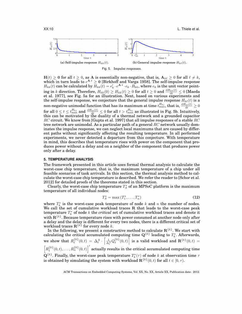
Based on the previous lemmata, we will show the first main result of this sectionin Theorem 5.4. A constructive algorithm is introduced to calculate the critical accu-mulated computing time Q

{k}` (0,∆) for all 0 ≤ ∆ ≤ τ that maximizes Tk,`(τ) at a

certain observation time τ , that is, Q{k}` (0,∆) leading to upper bound T ∗k,`(τ) ≥ Tk,`(τ).In particular, Algorithm 1 calculates the critical accumulated computing time Q{k}` byvarying both the position of the burst and the gap between burst and the first activeinterval. As sketched in Fig. 6, the critical accumulated computing time is the comput-ing time that maximizes the sum of the areas below the impulse response curve wherethe processing component is in ‘active’ processing mode. b`, ∆I

` , and ∆A` are defined as

in Section 4.1 and the auxiliary function v`(t, ζ) used in Algorithm 1 is one for ∆A` time

units, starting at time ζ.

THEOREM 5.4 (CRITICAL ACCUMULATED COMPUTING TIME). Suppose that thefunction v`(t, ζ) is defined as:

v`(t, ζ) =

{1 0 ≤ ζ ≤ t ≤ min(ζ + ∆A

` , τ)

0 otherwise(15)

and the accumulated computing time function Q{k}` (0,∆) for all 0 ≤ ∆ ≤ τ constructed

by Algorithm 1 leads to T ∗k,`(τ) at time τ . When the scheduler is work-conserving, T ∗k,`(τ)

is an upper bound on the highest value of Tk,`(τ) at time τ , that is, T ∗k,`(τ) ≥ Tk,`(τ).

So far, we only derived the accumulated computing time that maximizes the temper-ature at observation time τ . However, we did not dwell on the amount of observationtime τ . Next, we will show that increasing the observation time τ will not decreasethe worst-case peak temperature T ∗k if T0 ≤ (T∞)

i, where (T∞)i is the steady-state

temperature vector if all components are in ‘idle’ mode.

LEMMA 5.5 (INITIAL TEMPERATURE). Suppose that the accumulated computingtime function Q{k}(0,∆) for all 0 ≤ ∆ ≤ τ from Theorem 5.4 leads to the worst-casepeak temperature T ∗k (τ) at time τ . Then T ∗k (τ) ≥ Tk(t) for all 0 ≤ t ≤ τ and for any setof feasible workload traces with the same initial temperature vector T0 ≤ (T∞)

i.



time t [s] τ 0

Hk

ℓ(τ

-t)

1

Sℓ(t

)

bℓ - Δℓ

AΔℓ

IΔℓ

Ats

0 t(r)t(l)t Hkℓ

max~

pℓ

Fig. 6. Illustration of Algorithm 1 to calculate the critical accumulated computing time functionQ{k}` (0,∆).

5.2. Critical Accumulated WorkloadTheorem 5.4 provides an upper bound T ∗k,`(τ) on Tk,`(τ) at a certain observation time τ ,however, there might be no workload trace that leads to the critical accumulated com-puting time Q{k}` (0,∆). In the following, we will show that this is not the case, andR{k}` (0,∆) = ∆A

` ·⌈

1∆A

`

Q{k}` (0,∆)

⌉actually results in the critical accumulated comput-

ing time.

THEOREM 5.6 (CRITICAL CUMULATED WORKLOAD). Suppose that the accumu-lated computing time function Q{k}` (0,∆) for all 0 ≤ ∆ ≤ τ is defined as in Theorem 5.4.Then, the critical workload function R

{k}` (0,∆) = ∆A

` ·⌈

1∆A

`

Q{k}` (0,∆)

⌉— leads to the accumulated computing time Q{k}` (0,∆), and— complies with arrival curve α` according to Eq. (1).

Furthermore, the set of workload functions R{k}(0, t)

— leads to the highest possible temperature T ∗k (τ) ≥ Tk(t) for all 0 ≤ t ≤ τ and any set offeasible workload traces with the same initial temperature vector T0 ≤ (T∞)

i.

Suppose that the workload of all processing components is independent of each other.Then, the upper bound T ∗k (τ) determined by Theorem 5.6 is tight as there exists aworkload that leads to the critical accumulated computing time. Theorem 5.6 com-pleted the derivation of the constructive method to calculate the worst-case peak tem-perature T ∗k (τ) of component k. Starting from the set of arrival curves α(∆), we candetermine γ(∆) by Eq. (2). Afterwards, Algorithm 1 constructs Q{k}` for every com-ponent `, which in turn determines the critical sequence of ‘active’ and ‘idle’ modes.Finally, T ∗k (τ) can be found by solving the thermal model defined by Eq. (4) at timet = τ .

Finally note that the proposed thermal analysis method only calculates an upperbound on the maximum temperature inside the considered thermal model definedin Section 4.2. Its accuracy mainly depends on the selected granularity, that is, a higheraccuracy is obtained by dividing the floorplan in cells and individually measuring thetemperature of each cell [Skadron et al. 2004]. Another base assumption of our modelis the linear dependency of power dissipation on temperature due to leakage power. Asthis assumption is only valid inside a certain temperature range [Liu et al. 2007], itis critical to select the power parameters so that they upper bound the actual powerconsumption in the relevant temperature range.

6. AUTOMATIC GENERATION AND CALIBRATION OF ANALYSIS MODELSAutomation is the key for fast design space exploration. Design decisions are takenon the basis of comparing different system mappings and how well they perform withrespect to both timing and temperature. Integrating formal timing and thermal anal-



v1 v2 v3

c1 c2

n1

a1(1)

b1

n2

n3

b2

c1 c2

a2(1)

a2(2)

c1

a1 =

a1(1

)

b1

c2

b2

a2 =

a2

(1) +

a2

(2)

1

2

(a) Steps to calculate the computational demandof processing components. In particular, three pro-cesses v1, v2, and v3 are assigned to two processingcomponents χ1 and χ2.

0 10 20 30 400

10

20

30

40

α(1)ℓ

α(2)ℓ

α(3)ℓ

time interval ∆ [ms]

com

p.

dem

and

[m

s]

αℓ

α(1)ℓ + α

(2)ℓ + α

(3)ℓ

(b) Calculation of the arrival curve α` for process-ing component ` that has three processes assigned.α

(1)` , α(2)

` , and α(3)` are the arrival curves of the

corresponding processes.

Fig. 7. Analysis model generation.

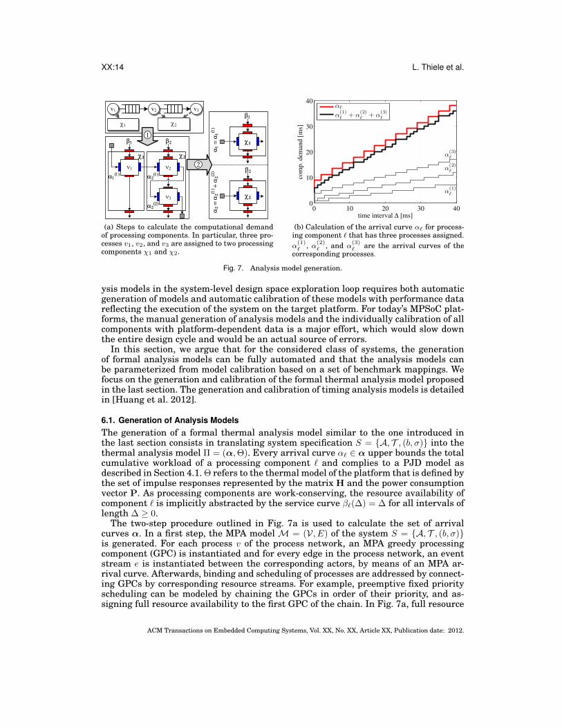
ysis models in the system-level design space exploration loop requires both automaticgeneration of models and automatic calibration of these models with performance datareflecting the execution of the system on the target platform. For today’s MPSoC plat-forms, the manual generation of analysis models and the individually calibration of allcomponents with platform-dependent data is a major effort, which would slow downthe entire design cycle and would be an actual source of errors.

In this section, we argue that for the considered class of systems, the generationof formal analysis models can be fully automated and that the analysis models canbe parameterized from model calibration based on a set of benchmark mappings. Wefocus on the generation and calibration of the formal thermal analysis model proposedin the last section. The generation and calibration of timing analysis models is detailedin [Huang et al. 2012].

6.1. Generation of Analysis ModelsThe generation of a formal thermal analysis model similar to the one introduced inthe last section consists in translating system specification S = {A, T , (b, σ)} into thethermal analysis model Π = (α,Θ). Every arrival curve α` ∈ α upper bounds the totalcumulative workload of a processing component ` and complies to a PJD model asdescribed in Section 4.1. Θ refers to the thermal model of the platform that is defined bythe set of impulse responses represented by the matrix H and the power consumptionvector P. As processing components are work-conserving, the resource availability ofcomponent ` is implicitly abstracted by the service curve β`(∆) = ∆ for all intervals oflength ∆ ≥ 0.

The two-step procedure outlined in Fig. 7a is used to calculate the set of arrivalcurves α. In a first step, the MPA model M = (V, E) of the system S = {A, T , (b, σ)}is generated. For each process v of the process network, an MPA greedy processingcomponent (GPC) is instantiated and for every edge in the process network, an eventstream e is instantiated between the corresponding actors, by means of an MPA ar-rival curve. Afterwards, binding and scheduling of processes are addressed by connect-ing GPCs by corresponding resource streams. For example, preemptive fixed priorityscheduling can be modeled by chaining the GPCs in order of their priority, and as-signing full resource availability to the first GPC of the chain. In Fig. 7a, full resource



availability is assigned to the GPC corresponding to v2, and the remaining resourceavailability is connected to the GPC of v3.

In the second step, the set of arrival curves α = [α1, . . . , αn]′ is calculated from thepreviously generated MPA model M = (V, E). Suppose that m actors are assigned toprocessing component `, each with arrival curve α(k)

` . Then the arrival curve α` is:

α`(∆) =

m∑k=1

α(k)` (∆). (16)

In case that α` is not anymore complying to the PJD model, it is necessary to convertthe arrival curve into the PJD model by the method presented in [Künzli et al. 2007].As the method upper bounds the original arrival curve, the proposed thermal analysismodel still leads to a safe bound on temperature. Figure 7b illustrates this step bymeans of a processing component that has three processes assigned.

The generation of the thermal model Θ follows directly from the platform specifica-tion. First, the coefficients φ, which reflect the temperature-dependency of the leakagepower, are calculated by linearizing the power model described in [Skadron et al. 2004].Then, the power consumption vector P is calculated by:

P(t) = φ ·(T(t)−Tbase

)+ Pleakage + Pdyn(t) = φ ·T(t) +ψ(t) (17)

where Tbase is the temperature vector for which the calibration parameters are ob-tained. The set of impulse responses is finally calculated by:

H(t) = eA·t ·B = e−C−1·(G+K−φ)·t ·C−1. (18)

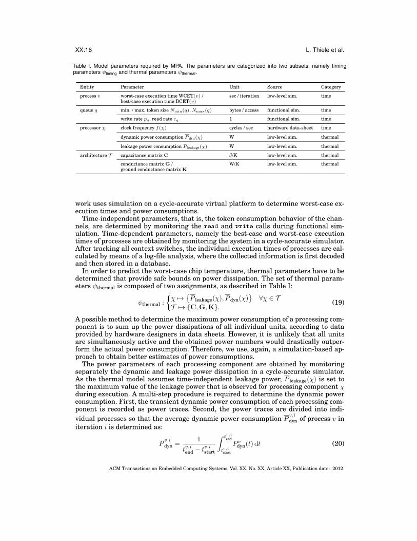
6.2. Calibration of Analysis ModelsDuring model generation, the timing behavior of a system is abstracted by arrival andservice curves. The thermal behavior is abstracted by a constant, but temperature-dependent, power consumption and a thermal RC network. In order to obtain the re-quired parameters for this abstraction, the application is calibrated prior to designspace exploration with data corresponding to the target platform. As model calibra-tion is specific to a certain model of computation, we restrict ourselves in this section toapplications specified using an SDF representation. Table I summarizes the requiredparameters and categorizes them into two subsets, namely timing parameters ψtimingand thermal parameters ψthermal. While timing analysis only depends upon the timingparameters ψtiming, both subsets are required for the calculation of the worst-case chiptemperature. Timing parameters include the worst-case and best-case execution timesof a process and the characteristics of the channels. The thermal parameters includethe power consumption and the thermal configuration of the platform.

Both the execution time of processes and the power consumption of processing com-ponents are associated with an uncertainty. Formal methods and tools [Wilhelm et al.2008] are actually required to calculate hard bounds on execution time and power con-sumption. However, such strict formal methods have the disadvantage that the overallmodeling effort drastically increases with the complexity of MPSoC platforms. An al-ternative for model calibration is simulation or execution on real hardware platforms.Although safe bounds cannot be guaranteed unless exhaustive test patterns are ap-plied, they are often the only practical possibility for model calibration. Compared toreal hardware platforms, simulation has the advantage that virtual platforms are of-ten earlier available and allow non-intrusive tracking of the execution. Therefore, inthe next section, the prototype implementation of the mapping optimization frame-



Table I. Model parameters required by MPA. The parameters are categorized into two subsets, namely timingparameters ψtiming and thermal parameters ψthermal.

Entity Parameter Unit Source Category

process v worst-case execution time WCET(v) /best-case execution time BCET(v)

sec / iteration low-level sim. time

queue q min. / max. token size Nmin(q), Nmax(q) bytes / access functional sim. time

write rate pq , read rate cq 1 functional sim. time

processor χ clock frequency f(χ) cycles / sec hardware data-sheet time

dynamic power consumption P dyn(χ) W low-level sim. thermal

leakage power consumption P leakage(χ) W low-level sim. thermal

architecture T capacitance matrix C J/K low-level sim. thermal

conductance matrix G /ground conductance matrix K

W/K low-level sim. thermal

work uses simulation on a cycle-accurate virtual platform to determine worst-case ex-ecution times and power consumptions.

Time-independent parameters, that is, the token consumption behavior of the chan-nels, are determined by monitoring the read and write calls during functional sim-ulation. Time-dependent parameters, namely the best-case and worst-case executiontimes of processes are obtained by monitoring the system in a cycle-accurate simulator.After tracking all context switches, the individual execution times of processes are cal-culated by means of a log-file analysis, where the collected information is first decodedand then stored in a database.

In order to predict the worst-case chip temperature, thermal parameters have to bedetermined that provide safe bounds on power dissipation. The set of thermal param-eters ψthermal is composed of two assignments, as described in Table I:

ψthermal :

{χ 7→

{P leakage(χ), P dyn(χ)

}∀χ ∈ T

T 7→ {C,G,K}. (19)

A possible method to determine the maximum power consumption of a processing com-ponent is to sum up the power dissipations of all individual units, according to dataprovided by hardware designers in data sheets. However, it is unlikely that all unitsare simultaneously active and the obtained power numbers would drastically outper-form the actual power consumption. Therefore, we use, again, a simulation-based ap-proach to obtain better estimates of power consumptions.

The power parameters of each processing component are obtained by monitoringseparately the dynamic and leakage power dissipation in a cycle-accurate simulator.As the thermal model assumes time-independent leakage power, P leakage(χ) is set tothe maximum value of the leakage power that is observed for processing component χduring execution. A multi-step procedure is required to determine the dynamic powerconsumption. First, the transient dynamic power consumption of each processing com-ponent is recorded as power traces. Second, the power traces are divided into indi-vidual processes so that the average dynamic power consumption P

v,i

dyn of process v initeration i is determined as:

Pv,i

dyn =1

tv,iend − tv,istart

∫ tv,iend

tv,istart

P vdyn(t) dt (20)



where tv,istart and tv,iend are the start and end time of iteration i, respectively. Then, we usethe maximum average value of Pdyn(t) as dynamic power consumption P dyn(χ):

P dyn(χ) = max∀v assigned to χ

(max∀i

(Pv,i

dyn

)). (21)

The thermal matrices G, S, and C are computed by means of the method describedin [Skadron et al. 2004]. The parameters required for this calculation, in particularthe three-dimensional floorplan and the thermal configuration of the chip, are knownfrom architecture specification.

In our mapping optimization framework, model calibration is performed just oncein the design flow, before design space exploration. As all functional parameters aremapping-independent, they only have to be obtained once for all candidate mappings.The same applies to the thermal configuration of the platform, that is, the G, K, andC matrices. All other parameters obtained by cycle-accurate simulation vary for eachcandidate mapping, but can be estimated by a set of benchmark mappings that coversall possible configurations. In the following experiments, we use the MPARM [Beniniet al. 2005] virtual platform for cycle-accurate simulation. As MPARM uses directmemory access controllers to reduce the interference between computation and com-munication, and all processing components are of the same type, the number of bench-mark mappings can be reduced to one.

7. EXPERIMENTSIn this section, a prototype implementation of the proposed system-level mapping op-timization framework is used to explore designs with respect to both worst-case tim-ing parameters and chip temperature. In the first case study, the viability of the pro-posed thermal analysis method is discussed by comparing the transient temperatureevolution for three different evaluation methods. Then, in the second case study, weevaluate the time to perform design space exploration and the quality of the obtainedtemperature bounds. Finally, the design space of two benchmark applications is ex-plored and Pareto optimal candidate mappings are identified in the third case study.The MPARM [Benini et al. 2005] cycle-accurate simulator is used in all experiments.

7.1. Experimental SetupA homogeneous multi-processor ARM platform with three processing components con-nected via a shared bus is considered as target platform. The MPA framework [Wan-deler et al. 2006] has been extended with the ability to calculate the worst-case chiptemperature by the method proposed in Section 5 and integrated into the prototypeimplementation of our mapping optimization framework to calculate the worst-casechip temperature and the overall latency of different candidate mappings.

Automated model calibration is performed based on timing and power numbers ex-tracted from MPARM virtual platform and thermal parameters from HotSpot [Huanget al. 2006], see Table II. In order to reduce the dimensionality of the search space,fixed priority preemptive scheduling is used on all processors while a TDMA policyis employed on the bus. However, our framework can easily be extended to considerother scheduling and arbitration policies, if they are available in the final system. Allexperiments have been performed on a 3.20 GHz Intel Pentium D machine with 2 GBof RAM.

7.2. Case Study ApplicationsIn this section, we analyze the timing and temperature behavior of four benchmarkapplications:



Table II. Thermal configuration of HotSpot.

Parameter Symbol Value

Silicon thermal conductance [W/(m ·K)] kchip 150Silicon specific heat [J/(m3 ·K)] pchip 1.75 · 106

Thickness of the chip [mm] tchip 3.5Convection resistance [K/W] rconvec 2Heatsink width [m] ssink 0.017Heatsink thickness [mm] tsink 0.01Heatsink thermal conductance [W/(m ·K)] ksink 400Heatsink specific heat [J/(m3 ·K)] psink 3.55 · 106

Thickness of the interface material [mm] tinterface 0.04Ambient temperature [K] Tamb 300

Producer-Consumer (P-C): The P-C example is a simple application that consists offive pipelined, parallel processes. The producer generates a stream of floating-pointnumbers, which are passed to the first worker process. After computing a few arith-metic operations, each worker process forwards the floating-point number to the nextworker process until the consumer receives it.

Motion-JPEG (MJPEG) decoder: The MJPEG decoder is a video codec in which eachvideo frame is separately compressed as a JPEG image. The MPA model of the consid-ered configuration is outlined in Fig. 8a. The decoder’s input (abstracted by the arrivalcurve αin) is a video stream that is first split into individual frames. The second actorsplits the frames into macroblocks to separately decode each macroblock. Afterwards,the decoded macroblocks are stitched together into a frame and finally into a stream.

Fast Fourier transform (FFT): In order to compute an 8-point FFT, a distributedlog(8)-stage butterfly network has been implemented [Wu and Chang 1993]. Eachstage is composed of four multiply-subtract-add modules so that the application canbe split up into twelve processes, each computing a multiply-subtract-add module.

Matrix multiplication: The distributed matrix multiplication application computesthe product of two N ×N matrices by subdividing the matrix product into single mul-tiplications and additions. This way, the application is split up into single processes,each performing a multiplication followed by an addition. To feed the structure and toretrieve the result, an input generator and an output consumer are added. Figure 8bshows the MPA model of the considered configuration for N = 2.

Split-

streamain

b3

Merge-

stream

De-

code

b1

Split-

frame

Merge-

frame

b2

(a) MJPEG decoder.

Gene-

ratorain

b3

Mult

0/0/1

b1

Mult

0/0/0

b2

Cons-

umer

Mult

0/1/1

Mult

0/1/0

Mult

1/0/1

Mult

1/0/0

Mult

1/1/1

Mult

1/1/0

(b) Matrix multiplication.

Fig. 8. Component model of the considered example applications. For the sake of simplicity, the componentmodel of the bus is not shown. αin abstracts the system’s input stream. β1, β2, and β3 abstract the availableresources of component χ1, χ2, and χ3, respectively.



0 1 2 3 4 5 6 7 8300

320

340

360 363.5K

time [s]

tem

per

atu

re [

K]

(a) MJPEG decoder, processing component 3.

0 1 2 3 4 5 6 7 8300

310

320

330

340

350 354.2K

time [s]

tem

per

atu

re [

K]

(b) Matrix multiplication, processing component 1.

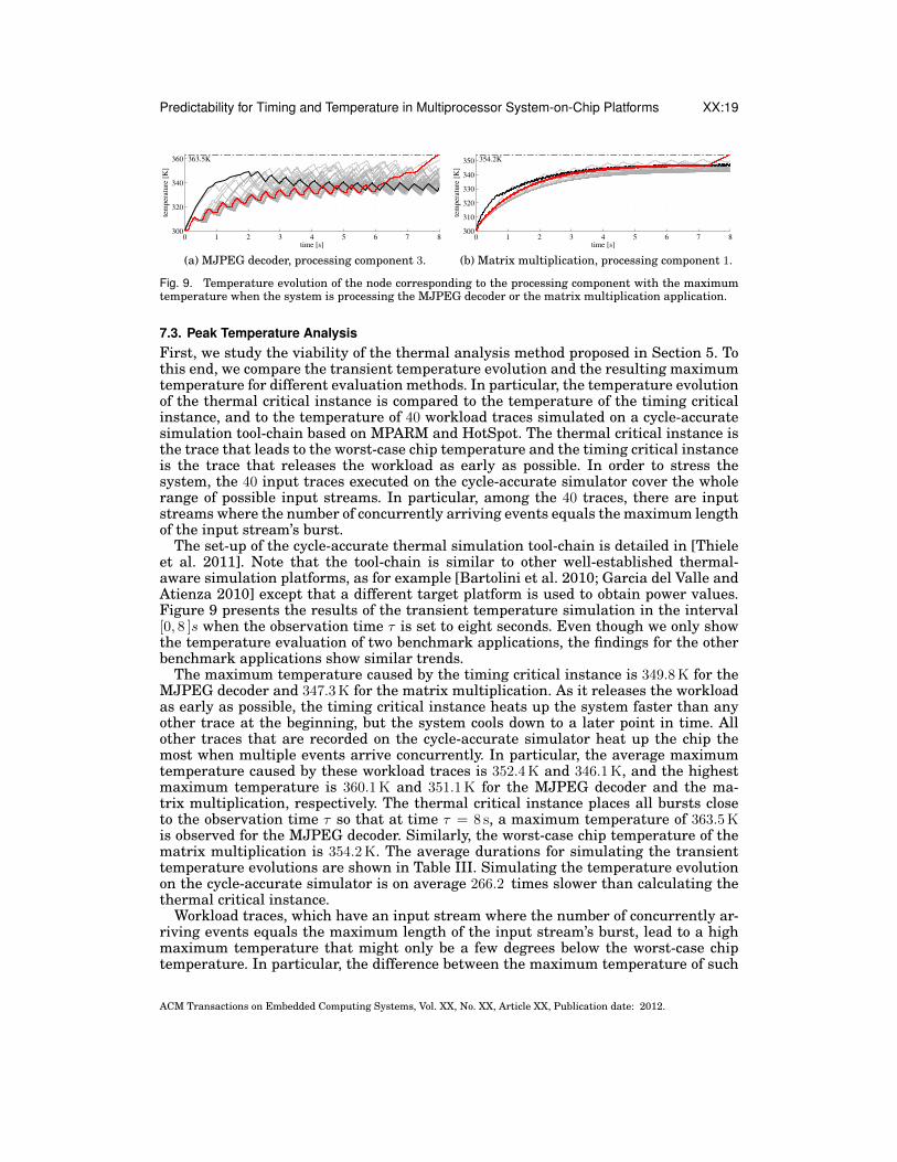
Fig. 9. Temperature evolution of the node corresponding to the processing component with the maximumtemperature when the system is processing the MJPEG decoder or the matrix multiplication application.

7.3. Peak Temperature AnalysisFirst, we study the viability of the thermal analysis method proposed in Section 5. Tothis end, we compare the transient temperature evolution and the resulting maximumtemperature for different evaluation methods. In particular, the temperature evolutionof the thermal critical instance is compared to the temperature of the timing criticalinstance, and to the temperature of 40 workload traces simulated on a cycle-accuratesimulation tool-chain based on MPARM and HotSpot. The thermal critical instance isthe trace that leads to the worst-case chip temperature and the timing critical instanceis the trace that releases the workload as early as possible. In order to stress thesystem, the 40 input traces executed on the cycle-accurate simulator cover the wholerange of possible input streams. In particular, among the 40 traces, there are inputstreams where the number of concurrently arriving events equals the maximum lengthof the input stream’s burst.

The set-up of the cycle-accurate thermal simulation tool-chain is detailed in [Thieleet al. 2011]. Note that the tool-chain is similar to other well-established thermal-aware simulation platforms, as for example [Bartolini et al. 2010; Garcia del Valle andAtienza 2010] except that a different target platform is used to obtain power values.Figure 9 presents the results of the transient temperature simulation in the interval[0, 8 ]s when the observation time τ is set to eight seconds. Even though we only showthe temperature evaluation of two benchmark applications, the findings for the otherbenchmark applications show similar trends.

The maximum temperature caused by the timing critical instance is 349.8 K for theMJPEG decoder and 347.3 K for the matrix multiplication. As it releases the workloadas early as possible, the timing critical instance heats up the system faster than anyother trace at the beginning, but the system cools down to a later point in time. Allother traces that are recorded on the cycle-accurate simulator heat up the chip themost when multiple events arrive concurrently. In particular, the average maximumtemperature caused by these workload traces is 352.4 K and 346.1 K, and the highestmaximum temperature is 360.1 K and 351.1 K for the MJPEG decoder and the ma-trix multiplication, respectively. The thermal critical instance places all bursts closeto the observation time τ so that at time τ = 8 s, a maximum temperature of 363.5 Kis observed for the MJPEG decoder. Similarly, the worst-case chip temperature of thematrix multiplication is 354.2 K. The average durations for simulating the transienttemperature evolutions are shown in Table III. Simulating the temperature evolutionon the cycle-accurate simulator is on average 266.2 times slower than calculating thethermal critical instance.

Workload traces, which have an input stream where the number of concurrently ar-riving events equals the maximum length of the input stream’s burst, lead to a highmaximum temperature that might only be a few degrees below the worst-case chiptemperature. In particular, the difference between the maximum temperature of such



Table III. Duration for simulating the transient temperature evolution for differentevaluation methods.

P-C MJPEG FFT Matrix

Thermal critical instance 84.8 s 94.3 s 83.0 s 90.5 sTiming critical instance 1.8 s 2.2 s 2.2 s 2.2 sCycle-accurate simulator 24876 s 22428 s 22873 s 23372 s

workload traces and the worst-case chip temperature may be caused due to severalreasons. First, the power consumption depends on various impact factors like cachemisses and bus congestions. Second, as shown in Section 5, the worst-case chip tem-perature results if all cores simultaneously process a specific pattern, which might bedifferent from a bursty input stream.

7.4. Efficiency and QualityAfter discussing the viability of the thermal analysis method, we integrate it into themapping optimization framework and measure its efficiency and quality. To this end,we first obtain the model parameters from executing the application with a bench-mark mapping. Afterwards, during design space exploration, these model parametersare used in different configurations to individually analyze every candidate mapping.To measure the efficiency, we compare the duration of analysis model generation, cal-ibration, and evaluation. In order to evaluate the quality of the obtained results, theworst-case chip temperature calculated by MPA is compared to the maximum tem-perature observed on a ten seconds system simulation using the previously describedcycle-accurate simulation tool-chain, and the maximum steady-state temperature cal-culated out of the average power consumption [Skadron et al. 2004]. Both methodscorrelate with the typical state-of-the-art thermal evaluation methods used in thermalaware task allocation and scheduling algorithms [Chantem et al. 2008; Xie and Hung2006].

The duration of analysis model generation, calibration, and evaluation are listed inTable IV. First, we note that calibration is two to three orders of magnitude slowerthan model generation and evaluation. Out of the three steps to perform model cali-bration, cycle-accurate simulation on MPARM is the most time consuming step. Theduration of the log-file analysis mainly depends on the number of context switches,which in turn depends on the number of processes. As a new log entry is created forevery context switch, the duration of the log-file analysis is long for the FFT applica-tion, where many dependent processes are concurrently executed. Furthermore, boththe duration of model calibration and the accuracy of the obtained results are affectedby the length of the execution trace. In general, longer execution traces increase the

Table IV. Duration of analysis model generation, calibration, and evaluation.

P-C MJPEG FFT Matrix

Model calibration Synthesis (incl. func. simulation) 37 s 58 s 47 s 39 s(one-time effort) Simulation on MPARM 24709 s 22504 s 22752 s 23510 s

Log-file analysis 114 s 114 s 1847 s 292 s

Overall time for one mapping 24861 s 22675 s 24646 s 23842 s

Design space Model generation 2 s 3 s 2 s 2 sexploration Model evaluation 96 s 132 s 96 s 119 s

Overall time for one mapping 98 s 135 s 98 s 121 s



360

350

340

330tem

per

atu

re [

K]

producer-consumer

320

MJPEG decoder

application / candidate mapping

370

1 2 3 4 5 6

FFT matrix multiplication

1 2 3 4 5 6 1 2 3 4 5 6 1 2 3 4 5 6

worst-case chip temp.

max. temp. from sim.

max. steady-state temp.

Fig. 10. Comparison of the worst-case chip temperature calculated by MPA, the maximum temperatureobserved on a ten seconds system simulation, and the maximum steady-state temperature for six candidatemappings per benchmark application.

calibration time but result in better calibration data with respect to worst-case execu-tion time and maximum average power consumption.

In Fig. 10, the worst-case chip temperature calculated by MPA is compared withthe maximum temperature observed on a ten seconds system simulation using thecycle-accurate simulation tool-chain and with the maximum steady-state temperature.Totally, we evaluated six randomly selected candidate mappings per benchmark appli-cation. The values are ordered by the maximum temperature of the system simulationin descending order, per benchmark application.

First, we note that the worst-case chip temperature always upper bounds the maxi-mum temperature obtained from cycle-accurate simulation. As cycle-accurate simula-tion is several orders of magnitude slower than formal thermal analysis, this confirmsour approach to include formal worst-case analysis models in the design space loop andto use cycle-accurate simulation only once for model calibration. Second, one can drawthe conclusion that the steady-state temperature is no indicator for a low worst-casechip temperature. Third, we note that a mapping candidate with a lower maximumtemperature from simulation does not necessary have a lower worst-case chip temper-ature. On the one hand, the maximum temperature of the cycle-accurate simulationunderestimates the worst-case chip temperature due to the infeasibility of an exhaus-tive simulation of all system configurations. On the other hand, the proposed thermalanalysis method does not lead to a tight bound on the maximum temperature of thesystem, due to several reasons:

— The parameters modeling the power consumption are the maximum average powerconsumption per iteration, thus overestimating the actual power consumption.

— The workload curves of the processing components are not independent of each otheras the component model results from a single process network.

— As not all arrival curves comply with a PJD model, original arrival curves have to beupper bounded.

Unlike simulation, the proposed thermal analysis method calculates a safe bound onthe maximum temperature of a candidate mapping. The difference between the worst-case chip temperature and the maximum temperature of the system simulation is theworst possible inaccuracy of the formal worst-case analysis method. Nonetheless, dueto the over-approximation of a tight bound on the maximum temperature of the sys-tem, another candidate mapping might actually have a lower maximum temperature.To avoid the selection of a wrong candidate mapping, the designer might keep more



340 345 350 355 360 365 3700

2

4

6

8

10

12

14

(1)

(2)

(3) (4)(5)

critical temperature

worst−case chip temperature [K]

wors

t−ca

se o

ver

all

late

ncy

[s]

(a) MJPEG decoder application.

350 352 354 356 358

2.9

3

3.1

3.2

3.3

3.4

3.5

3.6

(1)

(2)

(3)(4)

(5) (6)

critical temperature

worst−case chip temperature [K]

wors

t−ca

se o

ver

all

late

ncy

[m

s]

(b) Matrix multiplication application.

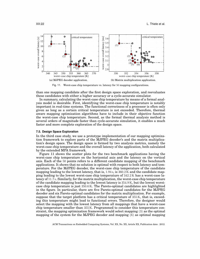
Fig. 11. Worst-case chip temperature vs. latency for 50 mapping configurations.

than one mapping candidate after the first design space exploration, and reevaluatesthese candidates with either a higher accuracy or a cycle-accurate simulator.

In summary, calculating the worst-case chip temperature by means of a formal anal-ysis model is desirable. First, identifying the worst-case chip temperature is notablyimportant in real-time systems. The functional correctness of a processor is often onlygiven as long as a certain critical temperature is not exceeded. Therefore, thermalaware mapping optimization algorithms have to include in their objective functionthe worst-case chip temperature. Second, as the formal thermal analysis method isseveral orders of magnitude faster than cycle-accurate simulation, it enables a muchfaster and more complete exploration of the design space.

7.5. Design Space ExplorationIn the third case study, we use a prototype implementation of our mapping optimiza-tion framework to explore parts of the MJPEG decoder’s and the matrix multiplica-tion’s design space. The design space is formed by two analysis metrics, namely theworst-case chip temperature and the overall latency of the application, both calculatedby the extended MPA framework.

Figure 11 shows the scatter plots for the two benchmark applications having theworst-case chip temperature on the horizontal axis and the latency on the verticalaxis. Each of the 50 points refers to a different candidate mapping of the benchmarkapplications. It shows that no solution is optimal with respect to both latency and tem-perature. For the MJPEG decoder, the worst-case chip temperature of the candidatemapping leading to the lowest latency, that is, 1.94 s, is 360.2 K and the candidate map-ping leading to the lowest worst-case chip temperature of 342.2 K has a worst-case la-tency of 11.7 s. Similarly, for the matrix multiplication, the worst-case chip temperatureof the candidate mapping leading to the lowest latency is 354.9 K, but the lowest worst-case chip temperature is just 350.6 K. The Pareto-optimal candidates are highlightedin the figure. In particular, there are five Pareto-optimal candidates for the MJPEGdecoder and six Pareto-optimal candidates for the matrix multiplication. For example,suppose that the target platform has a critical temperature of 355 K, that is, exceed-ing this temperature might lead to functional errors. Therefore, the designer wouldselect the mapping with the lowest latency from all mappings that have a worst-casechip temperature smaller than 355 K. Programmed to consider this temperature con-straint, the mapping optimization framework would select mapping (3) as the optimalmapping of the system for the MJPEG decoder and mapping (6) as optimal mapping



Split-

stream

ARM 1

Merge-

stream

De-

code

AR

M 3

Split-

frame

AR

M 2

Merge-

frame

(a)T ∗S = 342.2 K, l∗ = 11.7 s.

Split-

stream

ARM 2

Merge-

stream

De-

code

AR

M 3

Split-

frame

AR

M 1

Merge-

frame

(b)T ∗S = 350.6 K, l∗ = 11.7 s.

Split-

stream

ARM 1

Merge-

stream

De-

code

AR

M 3

Split-

frame

Merge-

frame

ARM 2

(c)T ∗S = 359.9 K, l∗ = 3.1 s.

Split-

stream

ARM 1

Merge-

stream

De-

code

AR

M 2

Split-

frame

Merge-

frame

ARM 3

(d)T ∗S = 358.2 K, l∗ = 3.1 s.

Split-

stream

ARM 1

Merge-

stream

De-

code

ARM 3

Split-

frame

ARM 2

Merge-

frame

(e)T ∗S = 364.5 K, l∗ = 2.4 s.

Split-

stream

ARM 1

Merge-

stream

De-

code

ARM 3

Split-

frame

ARM 2

Merge-

frame

(f)T ∗S = 365.0 K, l∗ = 2.4 s.

Split-

stream

ARM 1

Merge-

stream

De-

code

ARM 3

Split-

frame

ARM 2

Merge-

frame

(g)T ∗S = 360.2 K, l∗ = 2.9 s.

Split-

stream

ARM 1

Merge-

stream

De-

code

ARM 3

Split-

frame

ARM 2

Merge-

frame

(h)T ∗S = 360.5 K, l∗ = 2.9 s.

Fig. 12. Eight mapping configurations of the MJPEG decoder application together with their worst-casechip temperature T ∗S and their latency l∗.

for the matrix multiplication. As the proposed algorithm offers safe bounds, the sys-tem can safely execute the mapping without further involving other (dynamic) thermalmanagement strategies, which may lead to unpredictable behavior.

To study the connection between the worst-case chip temperature and worst-caselatency in greater detail, Fig. 12 outlines eight selected mapping configurations of theMJPEG decoder application together with their worst-case chip temperature T ∗S andtheir latency l∗. In order to study the effect of the placement, we study solution pairswhere only the placement of the processing components has changed. For example,mappings 12a and 12b, and mappings 12c and 12d are solution pairs. It shows thatthe physical placement cannot be ignored in temperature analysis. For example, map-pings 12a and 12b have almost the same latency, but their peak temperatures differby more than 8 K. Therefore, even if the mapping is already predefined, the system de-signer might reduce the temperature by selecting an appropriate physical placement.

8. CONCLUSIONSIn this article, a high-level optimization framework for mapping real-time applica-tions onto embedded MPSoC architectures is presented that guarantees the final per-formance and correct function of the system, considering both functional and non-functional properties. As high chip temperatures may lead to long-term reliabilityconcerns and short-term functional errors, providing guarantees on maximum tem-perature is as important as functional correctness and timeliness for embedded real-time systems. In order to include formal timing and thermal analysis in design spaceexploration, the analysis models are automatically generated from the same set ofspecifications as used for software synthesis. Afterwards, the analysis models are au-tomatically calibrated with performance data reflecting the execution of the system onthe target platform. The data is automatically obtained prior to design space explo-ration based on a set of benchmark mappings. The considered thermal analysis modelis able to address various thermal effects like the heat exchange between neighbor-ing processing components and temperature-dependent leakage power to accuratelymodel the thermal behavior of modern MPSoC architectures. Finally, the high-levelmapping optimization framework is applied to a multiprocessor ARM platform to vali-date the effectiveness of the approach based on four benchmark applications. It showsthat optimizing a system with respect to both performance and temperature will leadto major benefits.



REFERENCESATIENZA, D. ET AL. 2007. HW-SW Emulation Framework for Temperature-Aware Design in MPSoCs. ACM

Trans. Des. Autom. Electron. Syst. 12, 3, 1–26.BACIVAROV, I., HAID, W., HUANG, K., AND THIELE, L. 2010. Methods and Tools for Mapping Process Net-

works onto Multi-Processor Systems-On-Chip. In Handbook of Signal Processing Systems, S. S. Bhat-tacharyya, E. F. Deprettere, R. Leupers, and J. Takala, Eds. Springer, New York, NY, USA, 1007–1040.

BARTOLINI, A., CACCIARI, M., TILLI, A., BENINI, L., AND GRIES, M. 2010. A Virtual Platform En-vironment for Exploring Power, Thermal and Reliability Management Control Strategies in High-Performance Multicores. In Proc. Great Lakes Symposium on VLSI (GLSVLSI). ACM, Providence,Rhode Island, USA, 311–316.

BENINI, L., BERTOZZI, D., BOGLIOLO, A., MENICHELLI, F., AND OLIVIERI, M. 2005. MPARM: Exploringthe Multi-Processor SoC Design Space with SystemC. J. VLSI Signal Process 41, 2, 169–182.

BIRKHOFF, G. AND VARGA, R. S. 1958. Reactor Criticality and Nonnegative Matrices. J. Soc. Ind. Appl.Math. 6, 4, 354–377.

BROOKS, D. AND MARTONOSI, M. 2001. Dynamic Thermal Management for High-Performance Micropro-cessors. In Proc. Int’l Symposium on High-Performance Computer Architecture (HPCA). IEEE, Monter-rey , Mexico, 171–182.

CHANTEM, T., DICK, R. P., AND HU, X. S. 2008. Temperature-Aware Scheduling and Assignment forHard Real-Time Applications on MPSoCs. In Proc. Design, Automation and Test in Europe (DATE).ACM/IEEE, Munich, Germany.

COSKUN, A. K., ROSING, T. S., AND WHISNANT, K. 2007. Temperature Aware Task Scheduling in MPSoCs.In Proc. Design, Automation and Test in Europe (DATE). ACM/IEEE, Nice, France.

DONALD, J. AND MARTONOSI, M. 2006. Techniques for Multicore Thermal Management: Classification andNew Exploration. In Proc. Int’l Symposium on Computer Architecture (ISCA). IEEE, Boston, USA.

FRIEDLAND, B. 1986. Control Systems Design: An Introduction to State-Space Methods. McGraw-Hill, NewYork, NY, USA.

GARCIA DEL VALLE, P. AND ATIENZA, D. 2010. Emulation-Based Transient Thermal Modeling of 2D/3DSystems-on-Chip with Active Cooling. Microelectronics Journal 41, 10, 1–9.

GUPTA, R. ET AL. 1997. The Elmore Delay as a Bound for RC Trees with Generalized Input Signals. IEEETrans. Comput.-Aided Design Integr. Circuits Syst 16, 95–104.

HARDAVELLAS, N., FERDMAN, M., FALSAFI, B., AND AILAMAKI, A. 2011. Toward Dark Silicon in Servers.IEEE Micro 31, 4, 6–15.

HENIA, R., HAMANN, A., JERSAK, M., RACU, R., RICHTER, K., AND ERNST, R. 2005. System Level Per-formance Analysis - The SymTA/S Approach. IEEE Proc. Computers and Digital Techniques 152, 2,148–166.

HUANG, K., HAID, W., BACIVAROV, I., KELLER, M., AND THIELE, L. 2012. Embedding Formal PerformanceAnalysis into the Design Cycle of MPSoCs for Real-time Streaming Applications. ACM Trans. Embedd.Comput. Syst. 11, 1, 8:1–8:23.

HUANG, W., GHOSH, S., VELUSAMY, S., SANKARANARAYANAN, K., SKADRON, K., AND STAN, M. 2006.HotSpot: A Compact Thermal Modeling Methodology for Early-Stage VLSI Design. IEEE Trans. VeryLarge Scale Integr. (VLSI) Syst. 14, 5, 501–513.

KAHLE, J. A., DAY, M. N., HOFSTEE, H. P., JOHNS, C. R., MAEURER, T. R., AND SHIPPY, D. 2005. Intro-duction to the Cell Multiprocessor. IBM Journal of Research and Development 49, 4.5, 589 –604.

KANGAS, T., KUKKALA, P., ORSILA, H., SALMINEN, E., HÄNNIKÄINEN, M., HÄMÄLÄINEN, T. D., RI-IHIMÄKI, J., AND KUUSILINNA, K. 2006. UML-Based Multiprocessor SoC Design Framework. ACMTrans. Embedd. Comput. Syst. 5, 281–320.

KIENHUIS, B., DEPRETTERE, E., VISSERS, K., AND VAN DER WOLF, P. 1997. An Approach for Quantita-tive Analysis of Application-Specific Dataflow Architectures. In Proc. Int’l Conf. on Application-SpecificSystems, Architectures and Processors (ASAP). IEEE, Zurich , Switzerland, 338–349.

KRUM, A. 2000. Thermal Management. In The CRC Handbook of Thermal Engineering, F. Kreith, Ed. CRCPress, Boca Raton, FL, USA, 1–92.

KUMAR, A., SHANG, L., PEH, L., AND JHA, N. 2006. HybDTM: A Coordinated Hardware-Software Approachfor Dynamic Thermal Management. In Proc. Design Automation Conference (DAC). ACM, San Francisco,CA, USA, 548–553.

KÜNZLI, S., HAMANN, A., ERNST, R., AND THIELE, L. 2007. Combined Approach to System Level Perfor-mance Analysis of Embedded Systems. In Proc. Int’l Conf. on Hardware/Software Codesign and SystemSynthesis (CODES+ISSS). ACM, Salzburg, Austria.



LE BOUDEC, J.-Y. AND THIRAN, P. 2001. Network Calculus: A Theory of Deterministic Queuing Systems forthe Internet. Lecture Notes In Computer Science Series, vol. 2050. Springer, Berlin, Heidelberg.

LEE, E. AND MESSERSCHMITT, D. 1987. Synchronous Data Flow. Proc. IEEE 75, 9, 1235–1245.LIU, Y. ET AL. 2007. Accurate Temperature-Dependent Integrated Circuit Leakage Power Estimation is

Easy. In Proc. Design, Automation and Test in Europe (DATE). ACM/IEEE, Nice, France.LOH, G. H. 2008. 3D-Stacked Memory Architectures for Multi-core Processors. In Proc. Int’l Symposium on

Computer Architecture (ISCA). IEEE, Beijing, China, 453–464.MAEDA, H., KODAMA, S., AND KAJIYA, F. 1977. Compartmental System Analysis: Realization of a Class of

Linear Systems with Physical Constraints. IEEE Trans. Circuits and Systems 24, 1, 8–14.PAOLUCCI, P. S., JERRAYA, A. A., LEUPERS, R., THIELE, L., AND VICINI, P. 2006. SHAPES:: A Tiled Scal-

able Software Hardware Architecture Platform for Embedded Systems. In Proc. Int’l Conf. on Hard-ware/Software Codesign and System Synthesis (CODES+ISSS). ACM, Seoul, Korea, 167–172.

PIMENTEL, A. 2008. The Artemis Workbench for System-Level Performance Evaluation of Embedded Sys-tems. Int’l Journal on Embedded Systems 3, 3, 181–196.

RAI, D., YANG, H., BACIVAROV, I., CHEN, J.-J., AND THIELE, L. 2011. Worst-Case Temperature Analysisfor Real-Time Systems. In Proc. Design, Automation and Test in Europe (DATE). ACM/IEEE, Grenoble,France.

SCHOR, L., BACIVAROV, I., YANG, H., AND THIELE, L. 2012. Worst-Case Temperature Guarantees forReal-Time Applications on Multi-Core Systems. In Proc. IEEE Real-Time and Embedded Technologyand Applications Symposium (RTAS). IEEE, Beijing, China.

SKADRON, K., STAN, M. R., SANKARANARAYANAN, K., HUANG, W., VELUSAMY, S., AND TARJAN, D. 2004.Temperature-Aware Microarchitecture: Modeling and Implementation. ACM Trans. Architec. Code Op-tim. 1, 1, 94–125.

SRIDHAR, M., RAJ, A., VINCENZI, A., RUGGIERO, M., BRUNSCHWILER, T., AND ATIENZA ALONSO, D.2010. 3D-ICE: Fast Compact Transient Thermal Modeling For 3D-ICs with Inter-tier Liquid Cooling. InProc. Int’l Conf. on Computer-Aided Design (ICCAD). ACM/IEEE, San Jose, CA, USA, 463–470.

THIELE, L., BACIVAROV, I., HAID, W., AND HUANG, K. 2007. Mapping Applications to Tiled MultiprocessorEmbedded Systems. In Proc. Int’l Conf. on Application of Concurrency to System Design (ACSD). IEEE,Bratislava, Slovak Republic, 29–40.

THIELE, L., CHAKRABORTY, S., AND NAEDELE, M. 2000. Real-Time Calculus for Scheduling Hard Real-Time Systems. In Proc. IEEE Int’l Symposium on Circuits and Systems (ISCAS). Vol. 4. IEEE, Geneva,Switzerland, 101–104.

THIELE, L., SCHOR, L., YANG, H., AND BACIVAROV, I. 2011. Thermal-Aware System Analysis and SoftwareSynthesis for Embedded Multi-Processors. In Proc. Design Automation Conference (DAC). ACM, SanDiego, California, 268–273.

WANDELER, E., THIELE, L., VERHOEF, M., AND LIEVERSE, P. 2006. System Architecture Evaluation Us-ing Modular Performance Analysis: A Case Study. Int’l Journal on Software Tools for Technology Trans-fer 8, 6, 649–667.

WATANABE, Y., DAVIS, J. D., AND WOOD, D. A. 2010. WiDGET: Wisconsin Decoupled Grid Execution Tiles.In Proc. Int’l Symposium on Computer Architecture (ISCA). ACM, Saint-Malo, France, 2–13.

WILHELM, R. ET AL. 2008. The Worst-Case Execution-Time Problem – Overview of Methods and Survey ofTools. ACM Trans. Embedd. Comput. Syst. 7, 1–53.

WU, C.-W. AND CHANG, C.-T. 1993. FFT Butterfly Network Design for Easy Testing. IEEE Transactions onCircuits and Systems II: Analog and Digital Signal Processing 40, 2, 110–115.

XIE, Y. AND HUNG, W.-L. 2006. Temperature-Aware Task Allocation and Scheduling for Embedded Multi-processor Systems-on-Chip (MPSoC) Design. The Journal of VLSI Signal Processing 45, 3, 177–189.

YANG, C.-Y., CHEN, J.-J., THIELE, L., AND KUO, T.-W. 2010. Energy-Efficient Real-Time Task Schedul-ing with Temperature-Dependent Leakage. In Proc. Design, Automation and Test in Europe (DATE).ACM/IEEE, Dresden, Germany, 9–14.

ZHAO, M., CHILDERS, B. R., AND SOFFA, M. L. 2005. A Model-Based Framework: An Approach forProfit-Driven Optimization. In Proc. Int’l Symposium on Code Generation and Optimization (CGO).ACM/IEEE, San Jose, California, 317–327.

ZHU, C., GU, Z., SHANG, L., DICK, R., AND JOSEPH, R. 2008. Three-Dimensional Chip-Multiprocessor Run-Time Thermal Management. IEEE Trans. Comput.-Aided Design Integr. Circuits Syst 27, 8, 1479–1492.

Received November 2011; revised March 2012; accepted June 2012


xx predictability for timing and temperature in

Documents