1

CHAPTER ONE

INTRODUCTION

Objective

The main objective of the project is to design an antenna for local television stations in

the country that suits the local TV channels with varying element lengths. The quality of

reception is kept in mind where the length of elements are varied.

Problem definition

Currently in the country yagi antenna are used but they are made with no criteria or

design but pure imitation of foreign country antennas which operate on different TV

frequencies as compared to the Kenyans one. Through research it was noted that the

antennas in the country are made with over emphasis on cost effectiveness hence

compromising on the effectiveness of the antenna. TV stations in the country have their

transmitting stations in different points all over the country hence making the

transmission of radio electromagnetic waves difficult as we move away from the

transmitting antenna the RF signal becomes weak due to obstacles and interference from

other communication waves in the atmosphere hence the requirement of high gain

antennas with high directivity. The study of the yagi antenna was done where lengths of

the directors were varied with different constant spacing with the use of a solid and tubes

materials. Availability of the materials was considered in case of need of large scale

productions . Study of how to improve signal reception was done

size of elements was taken to consideration.

2

ANTENNA FUNDAMENTALS

Definition

An antenna is basically the structure associated with the transition between a guided

wave and free space wave or vice versa. An antenna is considered as a conversion device

or transducer which converts electrical energy in form of RF signal into electromagnetic

waves(transmitting antenna) and also intercepting the same electromagnectic waves to

produce a RF signal for the receiver input(receiving antenna) [1].The directional pattern

of a transmitting antenna is identical to its directional pattern as a receiving antenna,

provided that non-linear or unilateral devices are not employed. The conventional

antenna is a conductor, or system of conductors, that radiates or intercepts

electromagnetic wave energy. An ideal antenna has a definite length and a uniform

diameter, and is completely isolated in space. However, this ideal antenna is not realistic.

Many factors make the design of an antenna for a communications system a more

complex problem which include the height of the radiator above the earth, the

conductivity of the earth below it, and the shape and dimensions of the antenna.All of

these above factors affect the radiated-field pattern of the antenna in space. Another

problem in antenna design is that the radiation pattern of the antenna must be directed

between certain angles in a horizontal or vertical plane, or both.

Most practical transmitting antennas are divided into two basic classifications, hertz

(half-wave) antennas and marconi (quarter-wave) antennas. Hertz antennas are generally

installed some distance above the ground and are positioned to radiate either vertically or

horizontally. Marconi antennas Operate with one end grounded and are mounted

perpendicular to the Earth or to a surface acting as a ground. Hertz antennas are generally

used for frequencies above 2 megahertz. Marconi antennas are used for frequencies

below 2 megahertz and may be used at higher frequencies in certain applications. [2]

Current and voltage distribution on an antenna

A current through the antenna produces a magnetic field, and a charge on the antenna

produces an electric field. Figure 1-1 shows the current and voltage distribution on a half-

wave (Hertz) antenna. In view A, a Piece of wire is cut in half and attached to the

3

terminals of a high-frequency ac generator. The frequency Of the generator is set so that

each half of the wire is 1/4 wavelength of the output. The result is a common type of

antenna known as a dipole.

Figure 1-1.—Current and voltage distribution on an antenna.

At a given time the right side of the generator is positive and the left side negative. Like

charges repel Because of this, electrons will flow away from the negative terminal as far

as possible, but will be attracted to the positive terminal. View B shows the direction and

distribution of electron flow. The distribution curve shows that most current flows in the

4

center and none flows at the ends. The current distribution over the antenna will always

be the same no matter how much or how little current is flowing. However, current at any

given point on the antenna will vary directly with the amount of voltage developed by the

generator.

One-quarter cycles after electrons have begun to flow, the generator will develop its

maximum voltage and the current will decrease to 0. At that time the condition shown in

view C will exist. No current will be flowing, but a maximum number of electrons will be

at the left end of the line and a minimum number at the right end. The charge distribution

view C along the wire will vary as the voltage of the generator varies. Therefore, the

following conclusions may be draw:

1. A current flows in the antenna with an amplitude that varies with the generator

voltage.

2. A sinusoidal distribution of charge exists on the antenna. Every 1/2 cycle, the

charges reverse polarity

3. The sinusoidal variation in charge magnitude lags the sinusoidal variation in

current by 1/4 cycle.

The electromagnetic radiation from an antenna is made up of two components, the E field

and the H field. The two fields occur 90 degrees out of phase with each other. These

fields add and produce a single electromagnetic field. The total energy in the radiated

wave remains constant in space except for some absorption of energy by the Earth.

However, as the wave advances, the energy spreads out over a greater area and, at any

given point, decreases as the distance increases. Various factors in the antenna circuit

affect the radiation of these waves. In figure 1-2, for example, if an alternating current is

applied at the A end of the length of wire from A to B, the wave will travel along the wire

until it reaches the B end.

Wire

A B

½ wavelength

` Figure 1-2 a ½ wavelength wire.

5

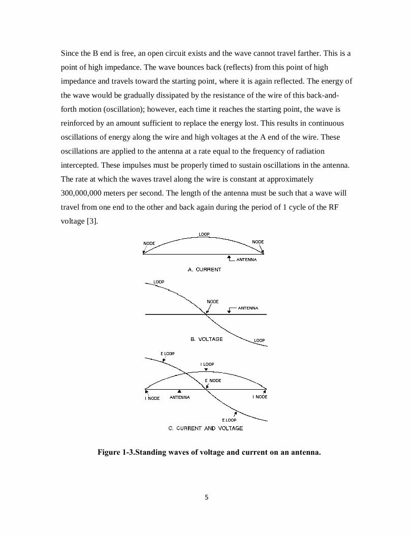
Since the B end is free, an open circuit exists and the wave cannot travel farther. This is a

point of high impedance. The wave bounces back (reflects) from this point of high

impedance and travels toward the starting point, where it is again reflected. The energy of

the wave would be gradually dissipated by the resistance of the wire of this back-and-

forth motion (oscillation); however, each time it reaches the starting point, the wave is

reinforced by an amount sufficient to replace the energy lost. This results in continuous

oscillations of energy along the wire and high voltages at the A end of the wire. These

oscillations are applied to the antenna at a rate equal to the frequency of radiation

intercepted. These impulses must be properly timed to sustain oscillations in the antenna.

The rate at which the waves travel along the wire is constant at approximately

300,000,000 meters per second. The length of the antenna must be such that a wave will

travel from one end to the other and back again during the period of 1 cycle of the RF

voltage [3].

Figure 1-3.Standing waves of voltage and current on an antenna.

6

Look at the current and voltage (charge) distribution on the antenna in figure 1-3.A

maximum movement of electrons is in the center of the antenna at all times; therefore, the

center of the antenna is at low impedance. This condition is called a standing wave of

current. The points of high current and high voltage are known as current and voltage

loops. The points of minimum current and minimum voltage are known as current and

voltage nodes. View A shows a current loop and current nodes. View B shows voltage

loops and a voltage node. View C shows the resultant voltage and current loops and

nodes. The presence of standing waves describes the condition of resonance in an

antenna. At resonance the waves travel back and forth in the antenna reinforcing each

other and the electromagnetic waves are transmitted into space at maximum radiation.

When the antenna is not at resonance, the waves tend to cancel each other and lose

energy in the form of heat [2].

ARRAY ANTENNAS

An array antenna is a special arrangement of basic antenna components involving new

factors and concepts. An array antenna is made up of more than one element, but the

basic element is generally the dipole. Sometimes the basic element is made longer or

shorter than a half-wave, but the deviation usually is not great [1].

A driven element is similar to the dipole connected directly to the transmission line. It

obtains its power directly from the transmitter or, as a receiving antenna; it delivers the

received energy directly to the receiver [1].

A parasitic element is located near the driven element from which it gets its power. It is

placed close enough to the driven element to permit coupling. A parasitic element is

sometimes placed so it will produce maximum radiation (during transmission) from its

associated driver. When it operates to reinforce energy coming from the driver toward it,

the parasitic element is referred to as a director. If a parasitic element is placed so it

causes maximum energy radiation in a direction away from itself and toward the driven

element, that parasitic element is called a reflector.If all of the elements in an array are

driven, the array is referred to as a driven array .If one or more elements are parasitic, the

entire system usually is considered to be a parasitic array. [1]

7

multielement arrays frequently are classified according to their directivity. a bidirectional

array radiates in opposite directions along the line of maximum radiation. A nidirectional

array radiates in only one general direction [1]

Arrays can be described with respect to their radiation patterns and the types of elements

of which they are made. Identify them by the physical placement of the elements and the

direction of radiation with respect to these elements. Broadside array designates an array

in which the direction of maximum radiation is perpendicular to the plane containing

these elements. In actual practice, this term is confined to those arrays in which the

elements themselves are also broadside, or parallel, with respect to each other. A

collinear array is one in which all the elements lie in a straight line with no radiation at

the ends of the array. The direction of maximum radiation is perpendicular to the axis of

the elements.[2&1]

End-fire array is one in which the principal direction of radiation is along the plane of

the array and perpendicular to the elements. Radiation is from the end of the array, which

is the reason this arrangement is referred to as an end-fire array. The currents in the

elements of the end-fire array are usually 180 degrees out of phase with each other as

indicated by the arrows in the figure. The construction of the end-fire array is like that of

a ladder lying on its side (elements horizontal). The dipoles in an end-fire array are closer

together (1/8-wavelength to 1/4 -wavelength spacing) than they are for a broadside array.

Closer spacing between elements permits compactness of construction. For this reason an

end-fire array is preferred to other arrays when high gain or sharp directivity is desired in

a confined space. However, the close coupling creates certain disadvantages. Radiation

resistance is extremely low, sometimes as low as 10 ohms, making antenna losses greater.

The end-fire array is confined mostly to narrow bandwidth. With changes in climatic or

atmospheric conditions, the danger of detuning exists [2].

Mutual impedance of an array

Antennas in an array couple to each other because they receive a portion of the power

radiated from nearby elements. This affects the input impedance seen by each element,

which depends on the array excitation. We scan a phased array by changing the feeding

coefficients, and this changes the element input impedance called the scan impedance. To

8

first order, the coupling or mutual impedance is proportional to the element pattern level

along the array face, and we reduce coupling by using narrower-beamwidth elements.

Figure 1-4.—typical end-fire array.

Mutual coupling can be represented by impedance, admittance, or scattering parameter

matrix.The first element of an N-element array has the impedance equation:

If we know the radiation amplitudes, we calculate the ratio of the currents:

1 132

11 12 13 11 1 1

....... NNV I

I IIZ Z Z Z

I I I= + + + +

The effective or scan impedance of the first element is:

321 11 12 13 1

1 1 1

1

1

....... NN

I IIZ Z Z Z Z

I I I

VI

+ + + += =

It depends on the self-impedance and the excitation of all the other antennas. The power

into the first element is

1 11 1 12 2 13 3 1....... N NV Z I Z I Z I Z I= + + + +

9

1 1

3211 12 13 1

1 1 1

* *1 1 1Re( .......) Re ....*N

NV I I II II

Z Z Z ZI I I

P = = + + + +

By knowing the feeding coefficients and the mutual impedances, we can compute the

total input power and gain. In general, every antenna in the array has different input

impedances. As the feeding coefficients change in a phased array to scan the beam, so

will the impedance of elements. The scan impedance change with scan angle causes

problems with the feed network. We can repeat the same arguments for slots using

mutual conductance, since magnetic currents are proportional to the voltage across each

slot.[4]

ANTENNA CHARACTERISTICS

Reciprocity of antenna

This property of interchangeability of the same antenna for transmitting and receiving is

known as antenna reciprocity because antenna characteristics are essentially the same for

sending and receiving electromagnetic energy. In general, the various properties of an

antenna apply equally, regardless of whether the antenna is used for transmitting or

receiving. The more efficient a certain antenna is for transmitting, the more efficient it

will be for receiving on the same frequency. Likewise, the directive properties of a given

antenna also will be the same whether it is used for transmitting or receiving. For

example, if a certain antenna used with a transmitter radiates a maximum amount of

energy at right angles to the axis of the antenna and minimum amount of radiation along

the axis of the antenna, as shown in figure 1-5, if this same antenna were used as a

receiving antenna, as shown in view B, it would receive best in the same directions in

which it produced maximum radiation; that is, at right angles to the axis of the antenna.

Polarization

The radiation field is composed of electric and magnetic lines of force. These lines of

force are always at right angles to each other. Their intensities rise and fall together,

reaching their maximums 90 degrees apart. The electric field determines the direction of

polarization of the wave. In a vertically polarized wave, the electric lines of force lie in a

10

vertical direction. In a horizontally polarized wave, the electric lines of force lie in a

horizontal direction.

Figure 1-5.—Reciprocity of antennas.

Circular polarization has the electric lines of force rotating through 360 degrees with

every cycle of RF energy. The electric field was chosen as the reference field because the

intensity of the wave is usually measured in terms of the electric field intensity (volts,

millivolts, or microvolts per meter). When a single-wire antenna is used to extract energy

from a passing radio wave, maximum pickup will result when the antenna is oriented in

the same direction as the electric field. Thus a vertical antenna is used for the efficient

reception of vertically polarized waves, and a horizontal antenna is used for the reception

of horizontally polarized waves. In some cases the orientation of the electric field does

not remain constant.Instead, the field rotates as the wave travels through space. Under

11

these conditions both horizontal and vertical components of the field exist and the wave

is said to have an elliptical polarization.[2]

Wavelength

Antenna size often refered relative to wavelength. For example: a half-wave dipole,

which is approximately a half-wavelength long. Wavelength is the distance a radio wave

will travel during one cycle. The formula for wavelength is:

cf

λ =

where f is the resonance frequency

83 10c m= × [speed of light]

Note: The length of a half-wave dipole is slightly less than a half-

wavelength due to end effect. The speed of propagation in coaxial cable is slower than in

air, so the wavelength in the cable is shorter. The velocity of propagation of

electromagnetic waves in coax is usually given as a percentage of free space velocity, and

is different for different types of coax.

Antenna bandwidth is an operating band of frequencies within the limits of which other

parameters do not exceed the limits of the tolerances called for by the technical

requirements.Usually, the parameter depending the most on frequency defines the limits

of the operating frequency band.For example, a change in the position of the radiation

pattern maximum, expansion of the beam and a drop in directive gain, and so on can

stipulate a frequency band limitation. [1]

Receiving antenna is one designed for reception of radio waves and conversion into

radio-frequency currents. The main characteristics of such an antenna are gain, directive

gain, effective area, antenna aperture efficiency, and frequency response.[1]

12

Broadband antenna is an antenna used for reception and transmission of signals in a

broad frequency band or on various frequencies. This type of antenna is capable of

operating with an upper and lower frequency ratio of up to 5:1 and more, with a slight

change in radiation pattern shape. Log periodic and helical antennas fall in this category.

These antennas sometimes are called frequency-independent antennas.[1]

Directivity.

It is a measure of the ability of an antenna to concentrate radiated power in a particular

direction .It measures the power density an actual antenna radiates in the direction of its

strongest emission, relative to the power density radiated by an ideal isotropic radiator

antenna radiating the same amount of total power [1]. Mathematically, the directivity is

defined as the maximum of the directive gain:

Where θ and φ are the standard spherical coordinate’s angles Radiated power density is

the power per unit solid angle such that

4π is the total solid angle for a sphere (also the surface area of a unit sphere, similar to 2π

being the total angle for a circle and the perimeter of a unit circle).

The denominator, , represents the average radiated

power density

directivity is expressed in dBi, so that

13

The reason the units are dBi (decibel relative to an isotropic radiator) is that for an

isotropic radiator, the radiated power density is a constant, and therefore equals the

average radiated power density (the denominator). This isotropic radiator is not directive

at all but has nevertheless a directivity stricto senso equal to 1. This can be misleading

and is much better described in dBi.

[6]

Antenna Gain

It is defined as the ratio of the radiation intensity of an antenna in a given direction to the

intensity that would be produced by a hypothetical ideal antenna that radiates equally in

all directions (isotropically) and has no losses. [1]Since the radiation intensity from a

lossless isotropic antenna equals the power into the antenna divided by a solid angle of 4п

steradians, we can write the following equation:

Although the gain of an antenna is directly related to its directivity, the antenna gain is a

measure that takes into account the efficiency of the antenna as well as its directional

capabilities. In contrast, directivity is defined as a measure that takes into account only

the directional properties of the antenna and therefore it is only influenced by the antenna

pattern. However, if we assumed an ideal antenna without losses then Antenna Gain will

equal directivity as the antenna efficiency factor equals 1 (100% efficiency). In practice,

the gain of an antenna is always less than its directivity.

14

The formulas above show the relationship between antenna gain and directivity, where

εcd = Prad / Pin is the antenna efficiency factor, D the directivity of the antenna and G the

antenna gain. In the antenna world, we usually deal with a “relative gain” which is

defined as the power gain ratio in a specific direction of the antenna, to the power gain

ratio of a reference antenna in the same direction. The input power must be the same for

both antennas while performing this type of measurement. The reference antenna is

usually a dipole, horn or any other type of antenna whose power gain is already

calculated or known.

In the case that the direction of radiation is not stated, the power gain is always calculated

in the direction of maximum radiation. The maximum directivity of an actual antenna can

vary from 1.76 dB for a short dipole, to as much as 50 dB for a large dish antenna. The

maximum gain of a real antenna has no lower bound, and is often -10 dB or less for

electrically small antennas.Taking into consideration the radiation efficiency of an

antenna; we can express a relationship between the antenna’s total radiated power and the

total power input as:

In the above formula, antenna radiation efficiency only includes conduction efficiency

and dielectric efficiency and does not include reflection efficiency as part of the total

efficiency factor. Moreover, the IEEE standards state that “gain does not include losses

arising from impedance mismatches and polarization mismatches”. Antenna Absolute

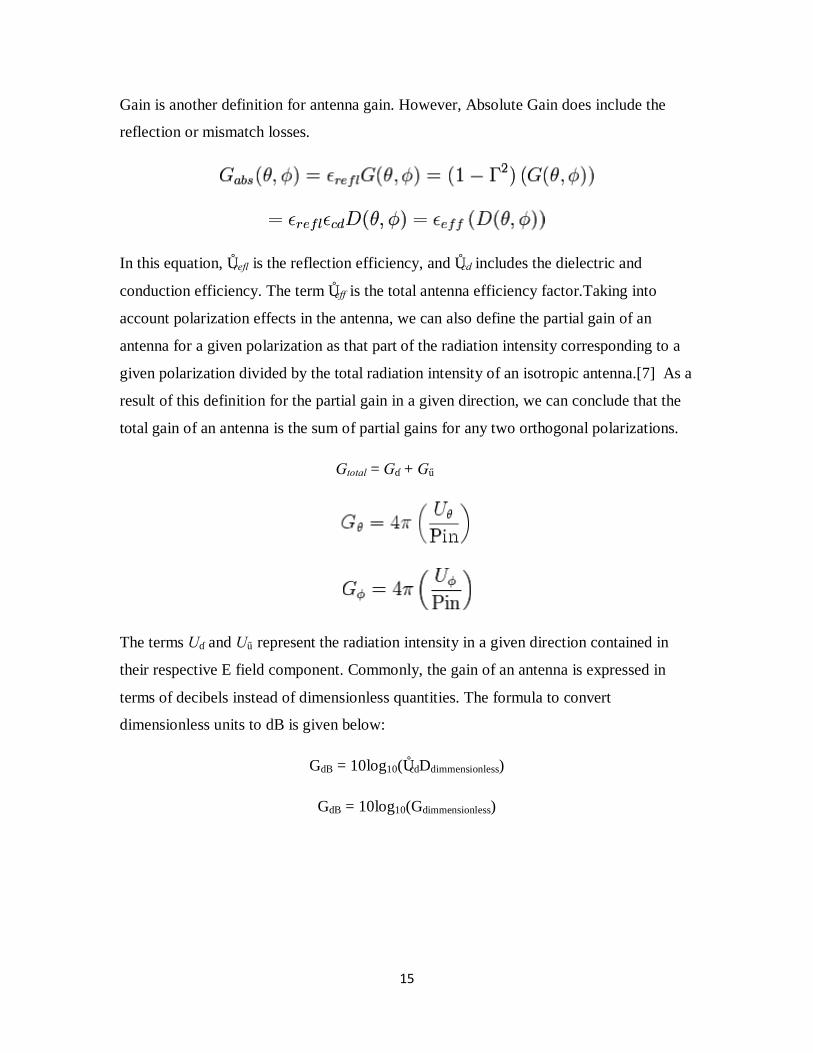
15

Gain is another definition for antenna gain. However, Absolute Gain does include the

reflection or mismatch losses.

In this equation, εrefl is the reflection efficiency, and εcd includes the dielectric and

conduction efficiency. The term εeff is the total antenna efficiency factor.Taking into

account polarization effects in the antenna, we can also define the partial gain of an

antenna for a given polarization as that part of the radiation intensity corresponding to a

given polarization divided by the total radiation intensity of an isotropic antenna.[7] As a

result of this definition for the partial gain in a given direction, we can conclude that the

total gain of an antenna is the sum of partial gains for any two orthogonal polarizations.

Gtotal = Gθ + Gφ

The terms Uθ and Uφ represent the radiation intensity in a given direction contained in

their respective E field component. Commonly, the gain of an antenna is expressed in

terms of decibels instead of dimensionless quantities. The formula to convert

dimensionless units to dB is given below:

GdB = 10log10(εcdDdimmensionless)

GdB = 10log10(Gdimmensionless)

16

Radiation pattern.

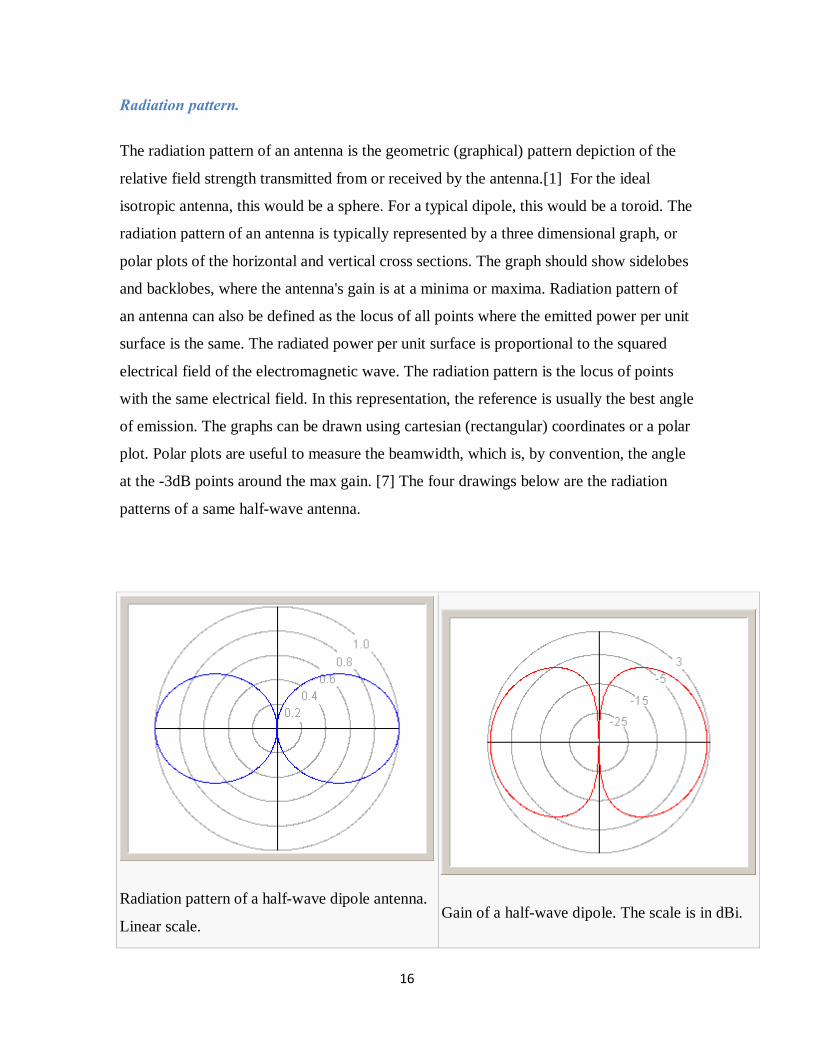
The radiation pattern of an antenna is the geometric (graphical) pattern depiction of the

relative field strength transmitted from or received by the antenna.[1] For the ideal

isotropic antenna, this would be a sphere. For a typical dipole, this would be a toroid. The

radiation pattern of an antenna is typically represented by a three dimensional graph, or

polar plots of the horizontal and vertical cross sections. The graph should show sidelobes

and backlobes, where the antenna's gain is at a minima or maxima. Radiation pattern of

an antenna can also be defined as the locus of all points where the emitted power per unit

surface is the same. The radiated power per unit surface is proportional to the squared

electrical field of the electromagnetic wave. The radiation pattern is the locus of points

with the same electrical field. In this representation, the reference is usually the best angle

of emission. The graphs can be drawn using cartesian (rectangular) coordinates or a polar

plot. Polar plots are useful to measure the beamwidth, which is, by convention, the angle

at the -3dB points around the max gain. [7] The four drawings below are the radiation

patterns of a same half-wave antenna.

Radiation pattern of a half-wave dipole antenna.

Linear scale.

Gain of a half-wave dipole. The scale is in dBi.

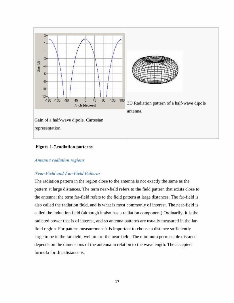
17

Gain of a half-wave dipole. Cartesian

representation.

3D Radiation pattern of a half-wave dipole

antenna.

Figure 1-7.radiation patterns

Antenna radiation regions

Near-Field and Far-Field Patterns

The radiation pattern in the region close to the antenna is not exactly the same as the

pattern at large distances. The term near-field refers to the field pattern that exists close to

the antenna; the term far-field refers to the field pattern at large distances. The far-field is

also called the radiation field, and is what is most commonly of interest. The near-field is

called the induction field (although it also has a radiation component).Ordinarily, it is the

radiated power that is of interest, and so antenna patterns are usually measured in the far-

field region. For pattern measurement it is important to choose a distance sufficiently

large to be in the far-field, well out of the near-field. The minimum permissible distance

depends on the dimensions of the antenna in relation to the wavelength. The accepted

formula for this distance is:

18

2

m in2 DR

λ=

Where minR is the minimum distance D is the largest dimension of the antenna and λ is the

wavelength.

When extremely high power is being radiated the near-field pattern is needed to

determine what regions near the antenna, if any, are hazardous to human beings.

Radiation resistance

Radiation resistance that part of an antenna's feedpoint resistance that is caused by the

radiation of electromagnetic waves from the antenna. The radiation resistance is

determined by the geometry of the antenna and not by the materials of which it is made.

19

It can be viewed as the equivalent resistance to a resistor in the same circuit. Radiation

resistance is caused by the radiation reaction of the conduction electrons in the

antenna.When electrons are accelerated, as occurs when an AC electrical field is

impressed on an antenna, they will radiate electromagnetic waves. These waves carry

energy that is taken from the electrons. The loss of energy of the electrons appears as an

effective resistance to the movement of the electrons, analogous to the ohmic resistance

caused by scattering of the electrons in the crystal lattice of the metallic conductor. While

the energy lost by ohmic resistance is converted to heat, the energy lost by radiation

resistance is converted to electromagnetic radiation. Power is calculated as:

P = I2R

where I is the electric current flowing into the feeds of the antenna and P is the power in

the resulting electromagnetic field. The result is that there is a virtual, effective

resistance:

This effective resistance is called the radiation resistance. Thus the radiation resistance of

an antenna is a good indicator of the strength of the electromagnetic field radiated by a

transmitting antenna or being received by a receiving antenna, since its value is directly

proportional to the power of the field. Electromagnetic theory employs Maxwell's

equations on a very small piece of the length of an antenna to determine the behavior of

that small increment and then uses integration to aggregate the behavior to that of the

entire antenna. As result the derivation gives the radiation resistance of a small (less than

a quarter wavelength) dipole antenna as

20

where is the length of the antenna in meters, λ is the wavelength of the signal in meters,

and R is measured in ohms. The radiation resistance of a half wave dipole in free space is

73 ohms.

Aperture is a surface, near or on an antenna, on which it is convenient to make

assumptions regarding the field values for the purpose of computing fields at external

points. More generally, the aperture of an antenna is its physical area projected on a plane

perpendicular to the mainbeam direction.[1]

Effective aperture a measure of the effective absorption area presented by the antenna

to the Incident wave. [1] If G receiving antenna gain, and the λ wavelength of the

radiation, then the effective aperture is 2

( , ) ( , )4eA Gλ

θ φ θ φπ

=

The aperture efficiency aη is defined as ea

AA

η = (dimensionless) where eA is the

effective aperture and A is the physical area of the antenna aperture.[1]

Front-to-back ratio

it is the ratio of the energy radiated in the principal direction compared to the energy

radiated in the opposite direction for a given antenna. The front-to-back ratio of an array

is the proportion of energy radiated in the principal direction of radiation to the energy

radiated in the opposite direction. A high front-to-back ratio is desirable because this

means that a minimum amount of energy is radiated in the undesired direction. Since

completely suppressing all such radiation is impossible, an infinite ratio cannot be

achieved. In actual practice, however, rather high values can be attained. Usually the

length and spacing of the parasitic elements are adjusted so that a maximum front-to-back

ratio is obtained, rather than maximum gain in the desired direction.[2]

21

CHAPTER 2

YAGI –UDA ANTENNA

The Yagi-Uda antenna is multielement parasitic array which was invented in 1926 by

Shintaro Uda of Tohoku Imperial University, Sendai, Japan, with the collaboration of

Hidetsugu Yagi, also of Tohoku Imperial University An antenna in which the gain of a

single dipole element is enhanced by placing a reflector element behind the dipole and

one or more director elements in front of it . The radiation from the different elements

arrives in phase in the forward direction, but out of phase by various amounts in the other

directions. The gain is slightly increased by the reflector and further enhanced by the first

director element. Additional director elements further increase the gain and improve the

front-to-back ratio, up to a point of diminishing returns. The director and the reflector in

the Yagi antenna are usually welded to a conducting rod or tube at their centers. This

support does not interfere with the operation of the antenna Since the driven element is

center-fed, it is not welded to the supporting rod which is the horizontal section between

all of the elements refered to as the boom. All of the elements usually lie in the same

plane. The center impedance can be increased by using a folded dipole as the driven

element. The folding concept is used to make the antenna self-resonant . The Yagi was

first widely used during World War II for airborne radar sets, because of its simplicity

and directionality .This type of antenna has traditionally been used for local television

reception. Its variants have found applications in the more modern communication

systems at higher frequencies and smaller sizes, and have even been adapted to printed-

circuit techniques in some applications. [8]

22

Figure 2-1.Structure of a yagi -uda

Since these antennas can be made highly directive with good radiation efficiency, they

have found new applications and new manufacturing techniques with miniaturization.

They can be printed on microwave circuit substrates with high dielectric constants, which

reduce their size even further. The parasitic electromagnetic coupling demonstrated in the

Yagi-Uda antenna has been adapted to many new types of miniaturized antennas

applicable to mobile communication devices in wide use, and will be used in future

wireless Internet devices.

THE DRIVEN ELEMENT

The driven element of a Yagi is the feed point where the feed line is attached from the

transmitter to the Yagi to perform the transfer of power from the transmitter to the

antenna. A dipole driven element will be resonant when its electrical length is 1/2 of the

wavelength of the frequency applied to its feed point. The feed point in the picture above

is on the center of the driven element.[8]

THE DIRECTOR

The directors are the shortest of the parasitic elements and this end of the Yagi is aimed

at the receiving station. It is resonant slightly higher in frequency than the driven element,

and its length will be about 5% shorter, progressively than the driven element. The

directors lengths can vary, depending upon the director spacing, the number of directors

used in the antenna, the desired pattern, pattern bandwidth and element diameter. The

23

numbers of directors that can be used are determined by the physical size (length) of the

supporting boom needed by your design. The directors are used to provide the antenna

with directional pattern and gain. The amount of gain is directly proportional to the

length of the antenna array and not by the number of directors used. The spacing of the

directors can range from 0.2 wavelength to 0.3 wavelength [9]

THE REFLECTOR

The reflector is the element that is placed at the rear of the driven element. It's resonant

frequency is lower, and typically slightly larger than resonant length of the driven

element by about approximately 5% longer. Its length will vary depending on the spacing

and the element diameter. The spacing of the reflector will be between .1 wavelengths

and .25 wavelengths. Its spacing will depend upon the gain, bandwidth, F/B ratio, and

sidelobe pattern requirements of the final antenna design. [9]

24

CHAPTER THREE

ANALYSIS OF A YAGI-UDA ANTENNA

The Yagi–Uda antenna functions as an endfire array, meaning that radiation is along the

axis of the array in the direction of the director elements. The nondriven, or parasitic,

reflector and director elements are excited through mutual coupling between themselves

and the fed dipole. Quantitative consideration of mutual coupling effects will show that

the current excited on the reflector element will lag in phase from the driven element

current, while the current excited on the director element leads in phase by approximately

the same amount. phase shifts are typically greater than the free-space phase delay

between the elements, so basic array theory [8] leads to the conclusion that the main

beam of the array will be in the direction of the director elements. Adding more reflector

elements to the left of the feed has little effect on the array, since radiation is

predominantly along the director elements. An increase in the number of directors

increases the directivity of the array, although this increase reaches the point of

diminishing returns after about 10–15 director elements. In general, the greater number of

parasitic elements used, the greater the gain. However, a greater number of such elements

causes the array to have a narrower frequency response as well as a narrower beamwidth.

Therefore, proper adjustment of the antenna is critical. The gain does not increase

directly with the number of elements used. For example, a three-element Yagi array has a

relative power gain of 5 dB. Adding another director results in a 2 dB increase.

Additional directors have less and less effect.[1]

Operation of yagi-uda as a parasitic array

The parasitic element is fed inductively by radiated energy coming from the driven

element. It is in NO way connected directly to the driven element.When the parasitic

element is placed so that it radiates away from the driven element, the element is a

director. When the parasitic element is placed so that it radiates toward the driven

element, the parasitic element is a reflector.The directivity pattern resulting from the

action of parasitic elements depends on two factors which are:

25

• the tuning, determined by the length of the parasitic element

• the spacing between the parasitic and driven elements.

To a lesser degree, it also depends on the diameter of the parasitic element. When a

parasitic element is placed a fraction of a wavelength away from the driven element and

is of approximately resonant length, it will re-radiate the energy it intercepts. The

parasitic element is effectively a tuned circuit coupled to the driven element, much as the

two windings of a transformer are coupled together. The radiated energy from the driven

element causes a voltage to be developed in the parasitic element, which, in turn, sets up

a magnetic field. This magnetic field extends over to the driven element, which then has a

voltage induced in it. The magnitude and phase of the induced voltage depend on the

length of the parasitic element and the spacing between the elements. In actual practice

the length and spacing are arranged so that the phase and magnitude of the induced

voltage cause a unidirectional, horizontal-radiation pattern and an increase in gain. In the

parasitic array in figure 3-1, view A, the parasitic and driven elements are spaced ¼

wavelength apart. The radiated signal coming from the driven element strikes the

parasitic element after 1/4 cycle. The voltage developed in the parasitic element is 180

degrees out of phase with that of the driven element. This is because of the distance

traveled (90 degrees) and because the induced current lags the inducing flux by 90

degrees (90 + 90 = 180 degrees). The magnetic field set up by the parasitic element

induces a voltage in the driven element 1/4 cycle later because the spacing between the

elements is 1/4 wavelength. This induced voltage is in phase with that in the driven

element and causes an increase in radiation in the direction indicated in figure 3-1, view

A. Since the direction of the radiated energy is stronger in the direction away from the

parasitic element (toward the driven element), the parasitic element is called a reflector.

The radiation pattern as it would appear if you were looking down on the antenna is

shown in view B. The pattern as it would look if viewed from the ends of the elements is

shown in view C. [2]

26

27

Figure 3-1 Patterns obtained using a reflector with proper spacing.

Because the voltage induced in the reflector is 180 degrees out of phase with the signal

produced at the driven element, a reduction in signal strength exists behind the reflector.

Since the magnitude of an induced voltage never quite equals that of the inducing

voltage, even in very closely coupled circuits, the energy behind the reflector (minor

lobe) is not reduced to 0.The spacing between the reflector and the driven element can be

reduced to about 15 percent of a wavelength. The parasitic element must be made

electrically inductive before it will act as a reflector. If this element is made about 5

percent longer than 1/2 wavelength, it will act as a reflector when the spacing is 15

percent of a wavelength. Changing the spacing and length can change the radiation

pattern so that maximum radiation is on the same side of the driven element as the

parasitic element. In this instance the parasitic element is called a director. Combining a

reflector and a director with the driven element causes a decrease in back radiation and an

increase in directivity. This combination results in the two main advantages of a parasitic

array which are unidirectivity and increased gain. If the parasitic array is rotated, it can

pick up or transmit in different directions because of the reduction of transmitted energy

in all but the desired direction due to unidirectivity. An antenna of this type is called a

rotary array. Size for size, both the gain and directivity of parasitic arrays are greater than

those of driven arrays. The disadvantage of parasitic arrays is that their adjustment is

critical and they do not operate over a wide frequency range. More gain and directivity

are obtained by changing the length of the parasitic elements.[2]

Mutual impendance of yagi

A Yagi–Uda antenna uses mutual coupling between standing-wave current elements to

produce a traveling-wave unidirectional pattern. It uses parasitic elements around the feed

element for reflectors and directors to produce an end-fire beam. Because the antenna can

be described as a slow wave structure , the directivity of a travelingwave antenna is

bounded when we include the directivity due to the element pattern. Maximum directivity

depends on length along the beam direction and not on the number of elements.

Consider two broadside-coupled dipoles. We describe the circuit relation between them

by a mutual impedance matrix:

28

Eq(3-1)

where the diagonal elements of the matrix are equal from reciprocity. If we feed one

element and load the other, we can solve for the input impedance of the feed antenna:

Eq(3-2)

where Z2 is the load on the second antenna. We short the second antenna (Z2 = 0) to

maximize the induced standing-wave current and eliminate power dissipation:

Eq(3-3)

The mutual impedance between broadside-coupled dipoles (Z12) approaches the self

impedance (Z11) as we move the dipoles close together and causes the input impedance

[Eq.(3-3)] to approach zero.The second equation of Eq. (3-1) for a shorted antenna relates

the currents in the two dipoles.

Eq(3-4)

Since Z12 ≈ Z22, the current in the shorted dipole is opposite the current in the feed

element, and radiation from the induced current reduces the fields around the dipoles.

Given the current on the parasitic element, we solve for the far field by array techniques.

When the elements are spaced a distance d, with the parasitic element on the z-axis and

29

the feed element at the origin, the normalized pattern response is;

Eq(3-5)

where Irejα = I2/I1 is the current of the parasitic element relative to the feed element. If

we take the power pattern difference between the pattern at θ = 0 and θ = 180◦,we get

Eq(3-6)

Case 1. δ = 180◦, E = 0, and we have equal pattern levels in both directions with a

null at θ = 90◦.

Case 2. 180◦ < δ < 360◦, E > 0. The parasitic element is a director, and the pattern in

its direction will be

higher (θ = 0) than at δ = 180◦.

Case 3. 0◦ < δ < 180◦,E < 0. The parasitic element is a reflector because the pattern

away from it (θ = 180◦) is higher than at θ = 0◦.

We look at the phase of the relative currents to determine whether a parasitic element is a

director or a reflector.

By use of these equations, Figure 3-2 was generated to show the phasing between a half-

wavelength dipole and a parasitic dipole as the length and spacing are varied. A parasitic

dipole of given length can be either a director or a reflector for different element spacing.

Generally, a director is somewhat shorter and a reflector is somewhat longer than the feed

element. If we reduce the length of the feed element or increase the element’s diameter,

the dividing line between a director and a reflector shifts upward. Figure 3-2 also shows

the decreased element length at the transition point for additional spaced elements.

With input matching we could increase the gain by 0.2 dB. A 3-dB gain bandwidth is

15% and a 1-dB gain bandwidth is 10%. At the 3-dB band edges the F/B ratio drops to

5.5 dB. As in many designs, the peak gain does not occur at the peak F/B value. The gain

rises by 0.2 dB to a 50-_ source at a point 3% higher in frequency than the point of

maximum F/B. The maximum gain with input impedance matching (8.6 dB) occurs at a

point 7% above the center frequency. The dipole element pattern narrows the E-plane

beamwidth and produces a null at 90◦ from the boresight. The traveling wave alone forms

30

the H-plane beam. A design to optimize the gain would have a phase progression along

the elements for short traveling-wave

Figure 3-2 Phase of current on a parasitic dipole relative to

current on a driven dipole.

31

Figure 3-3 Three-element Yagi–Uda dipole antenna.

Figure 3-3 illustrates a three-element Yagi–Uda dipole antenna having one reflector and

one director around the feed element. The design is a compromise between various

characteristics. With a 50-_ source its response is as follows:

Gain = 7.6 dB Front/back ratio = 18.6dB

Input impedance = 33 − j7.5 VSWR= 1.57 (50-_ system)

E-plane beamwidth = 64◦ H-plane beamwidth = 105◦

We analyze Yagi–Uda antennas by using the moment method [10]. One can calculate the

mutual impedance matrix:

[V ] = [Z][I ] Eq.(3-7)

The input voltage vector [V ] has only one nonzero term of the feed element. By solving

the linear equations Eq. (3-7), we compute the currents at the base of each element. We

assume a sinusoidal current distribution on each element and solve for the pattern

response from the array of dipoles. We calculate the input impedance of the array by

using the moment method; and by retaining the current levels on the dipoles for a known

input power, we can calculate gain directly.

32

Current distributions in yagi-uda array

Fig. 3-4Typical Yagi-Uda array.

A summarized integral-equation formulation for the currents in the N elements of a Yagi-

Uda array using a three-term approximation for the driven element and two terms with

complex coefficients for the parasitic elements is shown in this section [E]. The N

simultaneous Integral equations to be solved are

Where is the phase constant,V0k=0,for k =2,V02 is the excitation voltage of a

function generator in element 2

33

In solving the simultaneous integral equations (l), the current distributions I i ( z ) are

assumed to have the

Following form :

With

and Ai

(1) = 0, for i # 2. Substitution of (7) in (1) and use of certain approximate relations

for the integrals

involved yield

And two simultaneous matrix equations for the column matrices of complex coefficients

{A(2)} and {A(3)}:

geometrical dimensions are given, the complex coefficientsA2(1) ,{A(2)} and {A(3)}can be

determined from the equations

(11)-(13). With these coefficients known, the current distributions in all the dipole

elements of a Yagi-Uda array can be obtained from (7). We note that the mutual

coupling effects among the array elements are taken into consideration inherently in the

formulation and that the currents in the elements can deviate much form a

sinusoid[12],[13].

34

Length perturbation To adjust the element lengths in a Yagi-Uda array for maximum directivity it is assumed

that the length of the ith element be changed by a small amount maximum directivity it is

assumed that the length of the ith element be changed by a small amount ∆ hi( βo ∆ hi

<< 1).

The perturbed currents Ii p ( z ) Will be obtained from a modified version of (7) :

With

Where

A similar approximation can be applied to the distance terms Rki(hk) in (3) a.nd ( 5 ) , to

account for the change ∆ hk [11]. Perturbed definite integrals with element length in the

limits such as those in (1) and (2) may be written as follows:

With these approximations and t,he substitution of the perturbed currents I i p ( z ) in (1),

the matrices

35

and and the complex coefficients A2(1) and { A(m) } in (12) and

(13) are changed to , A 2 ( l ) p , and { A(m) } p ,

respectively. We have

The expressions for the deviation matrices in (22)-( 25) are quite complicated and will be

omitted here in order

to conserve space. They can be found in [SI. However, it is important, to note that, the

kith elements of the square deviation matrices in ( 22 ) and (23) and the kth elements of

the column deviation matrices in (24) and (2.5) can each be expanded as the sum of two

terms, both being proportional to the deviation in element length. For

example, the kith element of the deviation matrix in (22) can be written as

Where and can be evaluated from integrals containing

where the current deviation coefficients and are to be

determined.

In addition, the number \k22dc1) appearing in the denominator

of (11) will also be changed by length perturbation to

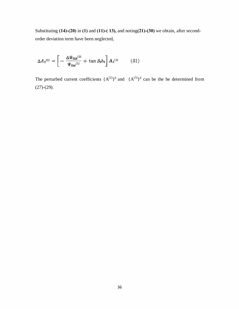
36

Substituting (14)-(20) in (1) and (11)-( 13), and noting(21)-(30) we obtain, after second-

order deviation term have been neglected,

The perturbed current coefficients {A(2)}p and {A(3)}p can be the be determined from

(27)-(29).

37

CHAPTER 4

DESIGN PROCEDURES

The design of the antenna system is very important in a transmitting station. The antenna

must be able to radiate efficiently so the power supplied by the transmitter is not wasted.

An efficient transmitting antenna must have exact dimensions. The dimensions are

determined by the transmitting frequencies. The dimensions of the receiving antenna are

not critical for relatively low radio frequencies. However, as the frequency of the signal

being received increases, the design and installation of the receiving antenna become

more critical. This chapter shows the design of the proposed Yagi antenna. From the

project statement, the main concern is to design and construct a yagi antenna to receive

signals from local TV station transmission. The first specification is therefore the

frequency in which the antenna is to be employed. Since the antenna is meant for ultra

high frequencies applications the frequency must lie within the range of 300Mhz to

3000Mhz.The design of the yagi antenna was approached in an experimental way where

using varying antenna lengths of the dipoles and constant space between the dipoles two

antennas where build where a solid dipoles and tube dipoles where used

Resonant length of an antenna

What is desired is that the antenna behaves as a resonant circuit at the frequency of

operation. it can be visualized that resonance shall occur when electrons travel from

centre to the end and back in a time equal to that occupied by one half of input cycle. The

conditions that satisfy this requirement are as flow Consider a centre fed antenna of

length l meters

'

sec

1 sec2

lt sc

t sf

=

=

't t= (for resonance)

38

12

2

lc f

clf

=

=

cfλ

= Where λ is the signal wavelength

2 22

2

c cl c c

l m

λ λ

λλ

= = =

=

Thus an antenna whose length is ( ( )2λ meters where λ is related to the frequency of the

applied signal by f= ( )c λ Will behave as a resonance resulting in large amplitude

voltages and currents and hence a powerful electromagnetic wave. [3]

Broadband design of yagi-uda

Several approaches to widening the inherently bandwidth of the yagi-uda array were used

which included:

• Shortening the directors for high frequency operations

• Lengthening the reflector for low frequency operations

• Selecting the driven dipole for midband operations

The parasitic elements are then used primary to increase gain at the upper and lower

frequency limits of the array Reflector and the driven elements are design for low

frequency and mid frequency.The local TV stations frequencies are shown figure 4-1

STATUS OF TV FREQUENCIES Identity TV Channel Station ID Frequency director length Status KBC 4 KBC channel 1 335.25 0.447 On Air Future Tech Electronics 9 Family TV 375.25 0.399 On Air DMTV 21

471.25 0.316 On Air

KBC 23 KBC channel 1 487.25 0.308 On Air KBC 29 K24 535.25 0.28 On Air

39

KBC 31 KBC Metro 551.25 0.272 On Air Royal Media Services 34 Citizen 575.25 0.261 On Air Royal Media Services 39 Citizen 615.25 0.244 On Air Nation Media Group 42 NTV 639.25 0.235 On Air Kitambo Communications 45 Aljazeera 663.25 0.226 On Air Capital Group 47 CNBC 679.25 0.221 On Air Stellavision 56 STV 751.25 0.199 On Air Lancia Media 57 Oxygen TV 759.25 0.198 On Air KTN Baraza Ltd 59 KTN 775.25 0.193 On Air Radio One IPP 62 EATV 799.25 0.188 On Air

mean

600.85

Figure 4-1 TV stations with their frequencies and calculated centre frequencies

The length (L) of the dipole was calculated as below Using the center frequency of

600.85

The length of the dipole or folded dipole required for resonance depends not only on the

frequency but also to a lesser extent on the ratio of the diameter of the element to the

wavelength

cf

λ = where

83 10c m= × [speed of light]

600.85f Mz= [centre frequency which is the mean average of the sum of all

tvs frequencies]

83 10 0.50600.85

mMHz

×λ = =

0.50 0.252 2L λ= = =

The reflector was calculated from data from table of figure where an average of the

frequencies below the centre frequencies was calculated as shown in figure 4-2

40

STATUS OF TV FREQUENCIES BELOW THE CENTRE FREQUENCY

Identity TV Channel Frequency Station ID Status

KBC 4 335.25 KBC channel 1 On Air

Future Tech Electronics 9 375.25 Family TV On Air

DMTV 21 471.25 On Air

KBC 23 487.25 KBC channel 1 On Air

KBC 29 535.25 K24 On Air

KBC 31 551.25 KBC Metro On Air

Royal Media Services 34 575.25 Citizen On Air

MEAN 475.8214286

Figure 4-2-calculation of the reflector resonant frequency

the wavelength of the reflector was calculated as below

83 10 0.6304475.82

m mMHz

λ ×= =

The length of the refector was as below

0.63 0.3152 2L mλ= = =

The lengths of the smallest director was calculated by the use of the highest frequency

799.25MGz

83 10 0.375799.25

m mMHz

λ ×= =

41

0.375 0.1872 2L mλ= = =

The lengths of the directors should vary between the length of dipole of 0.25m to the

smallest length due to the highest frequency of 0.187m.The director lengths of each TV

station frequency were calculated to give the general picture of suitable varying criteria

of the lengths. The lengths of the elements in the high-frequency array are shorter than

those in the low-frequency array as shown in figure 4-1.

For experimental and testing purpose, reduction of 2%,3% ,4%and 6% was chosen

The dipole length=0.25m

2% reduction we have

=0.02×0.25=0.005m

Resulted into twelve directors of length given by figure 4-3a

Directors D1 D2 D3 D4 D5 D6 D7 D8 D9 D10 D11 D12

Lengths(m) 0.245 0.240 0.235 0.230 0.225 0.220 0.215 0.210 0.205 0.200 0.195 0.190

Figure 4-3a Lengths of director with 2% reduction

3% reduction we have

=0.03×0.25=0.0075m

Resulted to eight directors of lengths given in the figure 4-3b

Directors D1 D2 D3 D4 D5 D6 D7 D8

Lengths(m) 0.2425 0.235 0.2275 0.2200 0.2125 0.205 0.1975 0.1900

Figure 4-3b Lengths of director with 3% reduction

42

4% reduction we have

=0.04×0.25=0.01m

Resulted to six directors of lengths given in the figure 4-3c

Directors D1 D2 D3 D4 D5 D6

Lengths .m 0.24 0.23 0.22 0.21 0.20 0.19

Figure 4-3cLengths of director with 4% reduction

6% reduction we have

=0.06×0.25=0.015m

Resulted to four directors of lengths given in the figure 4-3d

Directors D1 D2 D3 D4

lengths 0.235 0.22 0.205 0.19

Figure 4-3d Lengths of director with 3% reduction

Reflector to dipole spacing. A spacing of 0.25wavelength was used.

0.25×0.5=0.125m

This above spacing was chosen to achieve most reflection leading to a high gain

The spacing from dipole to director and between the director a spacing of 0.2 wavelength

was used to allow use of more directors. 0.2×0.5=0.1m

43

CONSTRUCTION

Materials used

• 12mm×12mm square aluminum tube

• 6.5mm solid aluminum rod

• 7.4mm aluminum tube(the only available in market)

• 75 Ohm RG-8 coax cable

• RP-TNC connectors for RG-8 cable

• Plastic insulators

• Bolts and nuts

• Plastic mould connector

Tools used:

• Steel Ruler

• Hack saw

• Flat file

• Hole Punch

• Soldering iron and solder

• Drill drill bit

• Rubber mallet

• Subscriber

• Venier caliper

• divider

Making the folded dipole

A round solid former was used to make corners at the folded dipole. The solid round rod

was hold tightly with the holding device and room was left for the bending of aluminum

44

rod. The first bend was made at the first marked point at one end. To make the first bend,

the mark was calculated exactly where the bend should begin, and the aluminum Straight

part was clamped and the free end tightly pulled around the former. The tube bends quite

easily without collapsing significantly. For the aluminum rod a soft mallet was used to

encourage the tubing to follow tightly around the former, especially towards the finish of

the bend. Care was taken in bending the tube to avoid it from collapsing. An allowance

was made for the spring off the bend from the former when marking out the bend at the

opposite end .when marking the second bend the two ends of the folded dipole were

ensured to be on the same plane. Some corrections were made by twisting. Some extra

length was left so that the ends of the tube and solid overlapped in the centre when the

dipole was folded. The exact centre was found and the ends were trimmed to give

allowance to the boom. Marks for the mounting holes to plastic connector were made

using a centre punch. An electrical drill with the right drilling bit was used to drill the

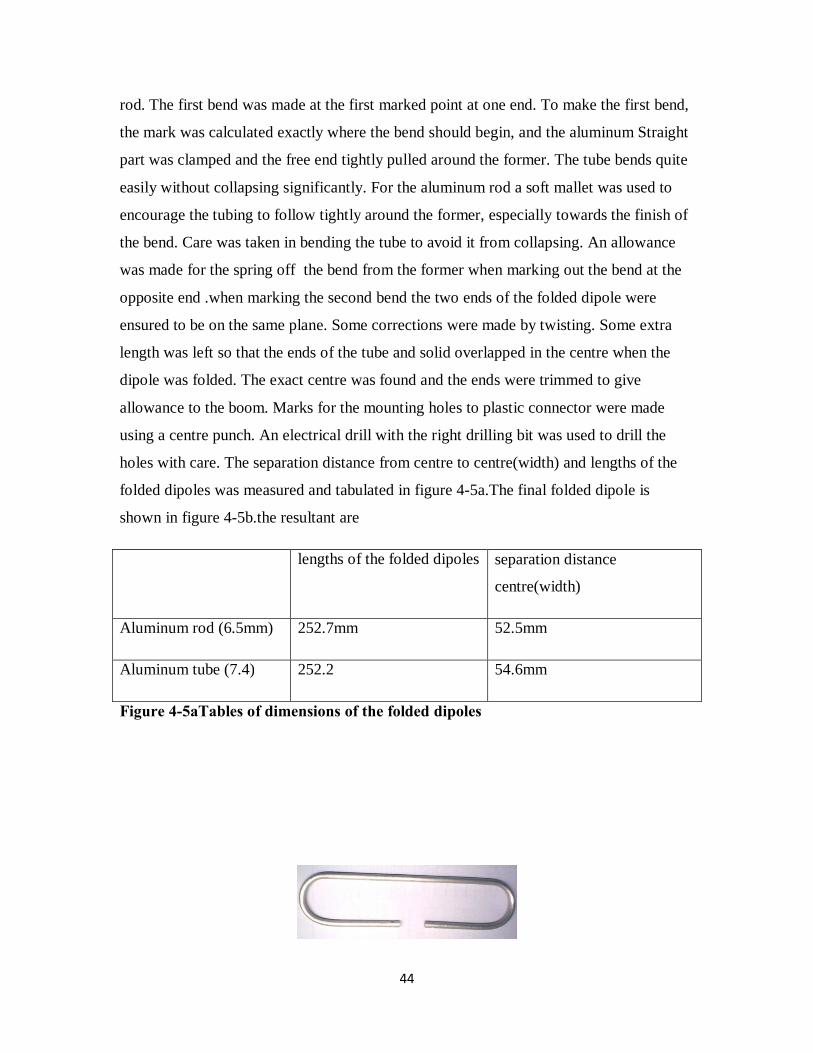
holes with care. The separation distance from centre to centre(width) and lengths of the

folded dipoles was measured and tabulated in figure 4-5a.The final folded dipole is

shown in figure 4-5b.the resultant are

lengths of the folded dipoles separation distance

centre(width)

Aluminum rod (6.5mm) 252.7mm 52.5mm

Aluminum tube (7.4) 252.2 54.6mm

Figure 4-5aTables of dimensions of the folded dipoles

45

Figure 4-5b Folded dipole

The plastic connector

A strong, thick walled plastic round connector with some screws wire holding was

purchased from suppliers. Two slots had to be made on the edges of the connector to

facilitate the fixing of the folded dipole using a square file. Two holes were made at a

marked distance to allow the fixing of the folded dipole on the plastic connector. Other

two holes were made to allow fixing of the plastic connector to the boom.

A B

Figure 4-6 showing the plastic connector(A) and a connected folded dipole

The trim ends of the folded dipole were soldered to the screws which allow tight

connection to the coaxial cable. When fixing the dipole care was taken to ensure that no

ground of electrical connection between the folded dipole and the boom as it will result in

unwanted RF currents running along the boom. The folded dipole was fixed in a way that

driven side was made to be on the same level plane with the parasitic elements.two vent

hole where made on the bottom of the plastic connector to allow it to ventilation and

avoid accumulation of rain water which can cause a connection to the boom ,short circuit

46

or so damage the coax flexible cable. The holes allows slow atmospheric corrosion as

moisture will get its way through.

Reflector

A plain ``sufuria sinia’’ was bought as it is made from aluminum for the parabolic

reflector. The diameter of the reflector was made to be 310mm.the centre was allocated

for cooking cover with the use of a scriber. Using a pencil and a plain A2 drawing paper

,the outer boundary was drawn on the papar giving its exact outer circle. The diameter of

the reflector was measured using a vernier caliper. Using the diameter arcs were made on

the circle dividing it into equal circumfrecial lengths and segments. The arcs exactly

opposite to each other were interlinked with straight lines. The intersection of the lines

gave the exact location of the centre. using the centre the inner diameter was divided

into five spaces by drawing circles with spacing of 2cm apart. The intersection between

these circles and the diagonal lines through the centre was used to make perforations on

the parabolic reflector. A centre punch was used to make drilling guides. Holes were

made by use of deferent sizes of drill bits starting from the smallest nice finish was

achieved by the use of a file and slight touch with bigger drill bits compared to the holes

to remove the debris.

Figure 4-7 The parabolic reflector

A hole slightly larger than the boom was made at the centre to avoid an electrical

connection to the boom and plastic insulator was joined to the reflector by using small

niles. The parabolic reflector is shown in figure 4-7

47

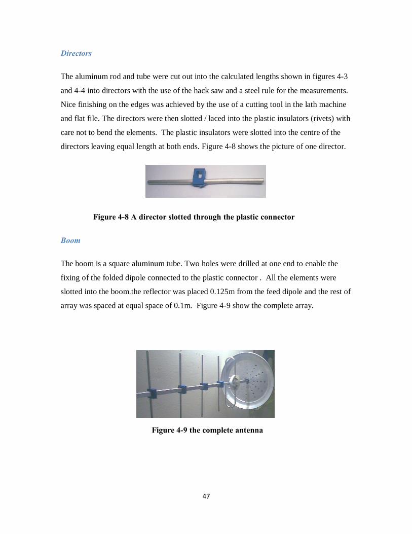
Directors

The aluminum rod and tube were cut out into the calculated lengths shown in figures 4-3

and 4-4 into directors with the use of the hack saw and a steel rule for the measurements.

Nice finishing on the edges was achieved by the use of a cutting tool in the lath machine

and flat file. The directors were then slotted / laced into the plastic insulators (rivets) with

care not to bend the elements. The plastic insulators were slotted into the centre of the

directors leaving equal length at both ends. Figure 4-8 shows the picture of one director.

Figure 4-8 A director slotted through the plastic connector

Boom

The boom is a square aluminum tube. Two holes were drilled at one end to enable the

fixing of the folded dipole connected to the plastic connector . All the elements were

slotted into the boom.the reflector was placed 0.125m from the feed dipole and the rest of

array was spaced at equal space of 0.1m. Figure 4-9 show the complete array.

Figure 4-9 the complete antenna

48

CHAPTER 5

SIMULATION RESULTS WITH SUPER NEC SOFT WARE

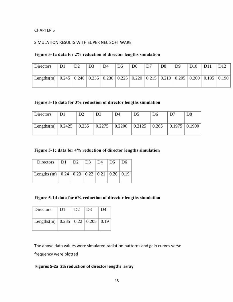
Figure 5-1a data for 2% reduction of director lengths simulation

Directors D1 D2 D3 D4 D5 D6 D7 D8 D9 D10 D11 D12

Lengths(m) 0.245 0.240 0.235 0.230 0.225 0.220 0.215 0.210 0.205 0.200 0.195 0.190

Figure 5-1b data for 3% reduction of director lengths simulation

Directors D1 D2 D3 D4 D5 D6 D7 D8

Lengths(m) 0.2425 0.235 0.2275 0.2200 0.2125 0.205 0.1975 0.1900

Figure 5-1c data for 4% reduction of director lengths simulation

Directors D1 D2 D3 D4 D5 D6

Lengths (m) 0.24 0.23 0.22 0.21 0.20 0.19

Figure 5-1d data for 6% reduction of director lengths simulation

Directors D1 D2 D3 D4

Lengths(m) 0.235 0.22 0.205 0.19

The above data values were simulated radiation patterns and gain curves verse

frequency were plotted

Figures 5-2a 2% reduction of director lengths array

49

The following radiation pattern was achieved at at test frequency of 501MGHs for the

2% reduction

Figures 5-2 b 2% reduction radiation pattern at 501MHz

Figure 5-2c

gain curve for

50

2% reduction of director lengths

At 2%

Maximum gain achieved 13.5dBi

Bandwidth at 13.5× 0.7071=9.55dBi

=543.75-412.5=131.25MHz has the smallest bandwidth but the largest gain of 13.5dBi

51

Figures 5-3a 3% reduction of length radiation pattern at 501MHz

52

Figure 5-3b gain curve of 3% reduction of lengths

At 3%

Maximum gain achieved =12dBi

Bandwidth at 0.7071×12=8.5dBi

=562-418=144MHz

The bandwidth improved with a reduction in the gain

53

Figures 5-4a array for 4% reduction of lengths

54

Figure 5-4b radiation pattern for 4% reduction at 501MHz

55

Figue 5-4c gain curve for 4% reduction of directors lengths

At 4% maximum gain achieved =11.5

Bandwidth at 0.7071×11.5=8.13dBi =556-410=146MHz

56

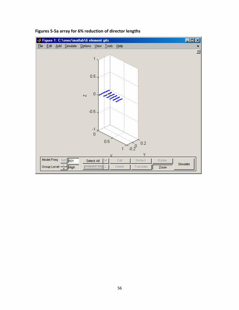
Figures 5-5a array for 6% reduction of director lengths

57

Figure 5-5b radiation pattern for 6% reduction at 501MHz

58

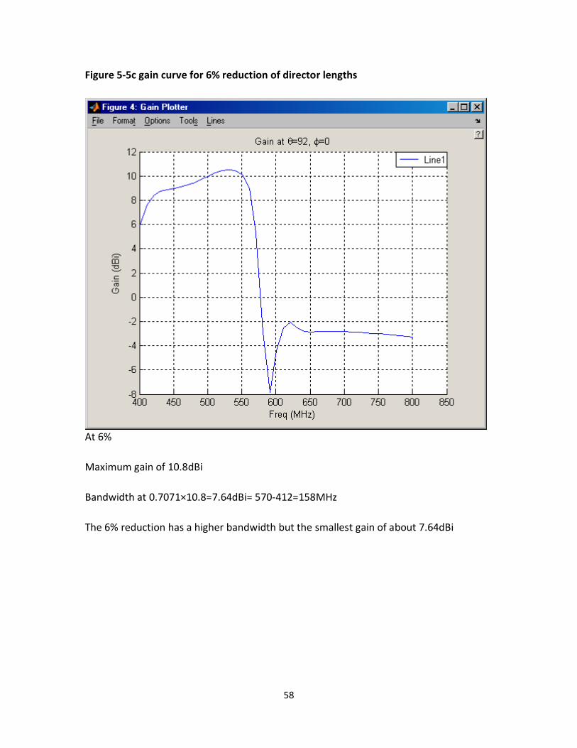
Figure 5-5c gain curve for 6% reduction of director lengths

At 6%

Maximum gain of 10.8dBi

Bandwidth at 0.7071×10.8=7.64dBi= 570-412=158MHz

The 6% reduction has a higher bandwidth but the smallest gain of about 7.64dBi

59

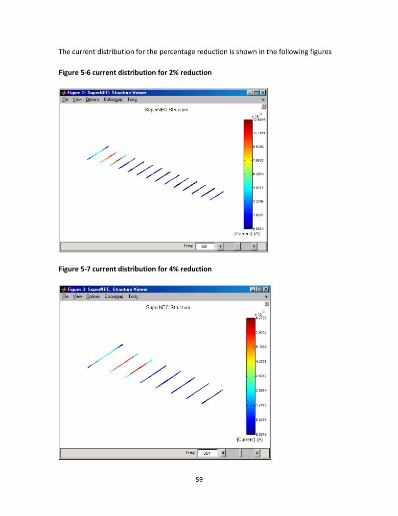
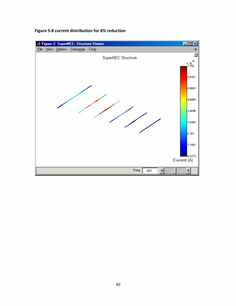
The current distribution for the percentage reduction is shown in the following figures

Figure 5-6 current distribution for 2% reduction

Figure 5-7 current distribution for 4% reduction

60

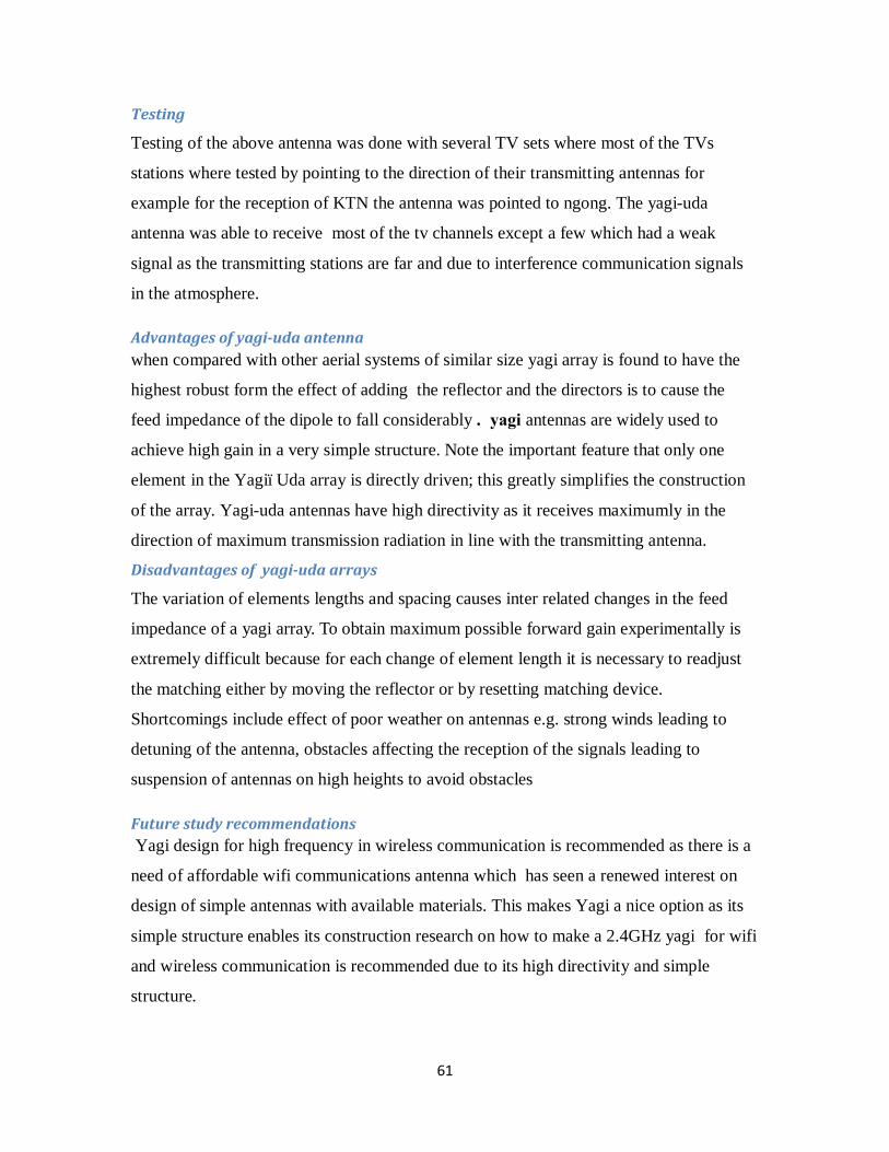
Figure 5-8 current distribution for 6% reduction

61

Testing

Testing of the above antenna was done with several TV sets where most of the TVs

stations where tested by pointing to the direction of their transmitting antennas for

example for the reception of KTN the antenna was pointed to ngong. The yagi-uda

antenna was able to receive most of the tv channels except a few which had a weak

signal as the transmitting stations are far and due to interference communication signals

in the atmosphere.

Advantages of yagi-uda antenna when compared with other aerial systems of similar size yagi array is found to have the

highest robust form the effect of adding the reflector and the directors is to cause the

feed impedance of the dipole to fall considerably . yagi antennas are widely used to

achieve high gain in a very simple structure. Note the important feature that only one

element in the Yagi–Uda array is directly driven; this greatly simplifies the construction

of the array. Yagi-uda antennas have high directivity as it receives maximumly in the

direction of maximum transmission radiation in line with the transmitting antenna.

Disadvantages of yagi-uda arrays The variation of elements lengths and spacing causes inter related changes in the feed

impedance of a yagi array. To obtain maximum possible forward gain experimentally is

extremely difficult because for each change of element length it is necessary to readjust

the matching either by moving the reflector or by resetting matching device.

Shortcomings include effect of poor weather on antennas e.g. strong winds leading to

detuning of the antenna, obstacles affecting the reception of the signals leading to

suspension of antennas on high heights to avoid obstacles

Future study recommendations Yagi design for high frequency in wireless communication is recommended as there is a

need of affordable wifi communications antenna which has seen a renewed interest on

design of simple antennas with available materials. This makes Yagi a nice option as its

simple structure enables its construction research on how to make a 2.4GHz yagi for wifi

and wireless communication is recommended due to its high directivity and simple

structure.

62

CONCLUSION As the reduction percentage of the lengths is varied from 2% to 6% as seen from the

simulation results the gain, directivity, bandwidth and no of elements changes. The

number of elements reduces as the percentage is increased because the shortest length

of the last director due to the highest frequency remains the same. The reduction in the

number of elements leads to a reduction in gain and directivity. The 6% reduction had

the largest bandwidth as it had low directivity.2% reduction had the highest gain of

13.5dBi but smallest bandwidth while the 4% reduction had a moderate gain 11.5dBi

and a large bandwidth making it suitable for yagi antenna. Reduction greater than 6%

leads to poor yagi as the coupling is reduced significantly.

The bandwidth of the antenna reduces with 2% reduction as it has the most elements

hence high gain and directivity narrowing the bandwidth.

From the TV test the directivity of the yagi antenna is high as the antenna reception

improved significantly with the pointing of the antenna in line with the transmitting

antennas. The 2% reduction antenna had the highest directivity as it had most number

of elements. the 6% had least directivity as it had the least number of elements.

63

REFERENCES

[1] IEEE Standard Definitions of Terms for Antennas

[2] Introduction to Wave Propagation, Transmission Lines, and Antennas NAVEDTRA 14182

[3] colour television and video technology by A.K.Maini second edition

[4] MODERN ANTENNA DESIGN Second Edition THOMAS A. MILLIGAN IEEE PRESS A JOHN

[5]VHF-UHF MANUAL by G.R. JESSOP

[6] Antenna Theory (3rd edition), by C. Balanis, Wiley, 2005, ISBN 0-471-66782-X

[7] Antenna for all applications (3rd edition), by John de Kraus, Ronald J. Marhefka, 2002, ISBN 0-07-232103-2

[8]H .Yagi, Beam transmission of ultra-short waves , Proceedings of the IRE, vol. 16, pp. 715-740, June 1928. The URL is to a 1997 IEEE reprint of the classic article.

[9]See also Beam Transmission Of Ultra Short Waves: An Introduction To The Classic Paper By H. Yagi by D.M. Pozar, in Proceedings of the IEEE, Volume 85, Issue 11, Nov. 1997 Page(s):1857 - 1863.

[10] C. S. Liang and Y. T. Lo, A multiple-field study for the multiarm log-spiral antennas,IEEE Transactions on Antennas and Propagation, vol. AP-16, no. 6, November 1968,pp. 656–664.

[11] C.S. CHEN,``Perturbation tachniques for directivity optimization of yagi-uda arrays,’’Phd. Dissertation,Syracuse university, Syracuse,N.Y.;1974

[12]R.W.P.King,R.B.Mack and S.S.Sandler, Arrays of Cylindrical Dipoles. New York: Cambridge,1968

[13]D.K. Cheng and C.A.Chen, ``Optamum element spacings for Yagi-Uda,” Syracuse university, Syracuse,N.Y.,Tech Rep. TR-72-9,Nov.1972.

64