year of publication:- of parameters for numerical... · muir wood, mackenzie and chan the cam clay...

~ Authors:-

Muir Wood, Do, Mackenzie, NoL. and Chan, A.H.C.

SELECTION OF PARAMETERS FOR NUMERICALPREDICTIONS

publication:-

PREDICTIVE SOil MECHANICS, PROCEEDINGS OF THEWROTH MEMORIAL SYMPOSIUM ST CATHERINE'S

COllEGE, OXFORDpp496-512

Year of publication:-

1992

REPRODUCED WITH KIND PERMISSION FROM:Thomas Telford Services Ltd

Thomas Telford House1 Heron Quay

London E144JD

Selection of parameters fornumerical predictions

D. MUIR WOOD, N.L. MACKENZIE and A.H.C. CHANDepartment of Civil Engineering, Glasgow University

Data from a test on reconstituted kaolin performed under axially symmetricstress conditions in a true triaxial apparatus are used to generate sets of values ofsoil parameters for use with the (modified) Cam clay model. First, parameters arechosen by the traditional route, one at a time: slope of normal compression lineand slope of unloading line in the compression plane, crItical state stress ratio,and elastic property. This fails to take any direct account of the shear strains thatoccur and yet it is in order to predict the response of a soil to shearing that amodel such as Cam clay is normally applied. An alternative procedure adopts anoptimisation strategy to produce a simultaneous best fit set of all parameters inorder to match any section or sections of the test that are reckoned to be ofimportance. The values of the parameters thus deduced are rather different, butthe mod:!l reproduces the soil behaviour more accurately.

IntroductionThe Cam clay models have become firmly established in the language ofsoil mechanics since their first introduction some thirty years ago(Roscoe and Schofield, 1963; Roscoe and Burland, 1968). Over the pasttwo decades, in particular, they have been widely used in numericalanalysis of geotechnical structures, especially those involving the load-ing of soft normally consolidated or lightly overconsolidated clays(Wroth, 1977). The Cam clay models have an important pedagogic roleto play in illustrating the way in which rather simple but completemodels of soil behaviour can be developed by a logical extension fromconsideration of ideas of yielding and plastic hardening of ductile metals(Schofield and Wroth, 1968; Muir Wood, 1990). The appeal of the Camclay models lies in their compactness, in the very small number of soilparameters - five, plus permeability - that are necessary for acomplete definition of the models, and in the physical basis of all theseparameters. The Cam clay models formed a central element of a numberof courses on Critical State Soil Mechanics that were presented in Britainand Europe between 1975 and 1985 (Wroth et al., 1975, 1979, 1981, 1982,1985) and much was always made of the fact that the five parameterswere not really new parameters, but familiar quantities seen in a new

496 Predictive soil mechanics. Thomas Telford, London, 1993

,

PARAMETERS FOR NUMERICAL PREDICTIONS

(truer) light. Thus the slope M of the critical state line in the p':qeffective stress plane is linked with the angle of shearing resistance q,';the slopes A, K of normal compression and unload-reload lines in thev:ln p' compression plane are linked with compression and swellingindices C~, C~; the location of the critical state line in the compressionplane is defined by a reference specific volume r which can be linkedwith liquid limit WL; and some second elastic property is required suchas shear modulus G or Poisson's ratio v. The model takes care of therest.

The continuation of this sales tactic is therefore that no special testsare required to determine the values of the soil parameters: testing cancontinue as before and the five parameters can be picked off one by one.

The fundamental feature of these soil models - and the vital messageof critical state soil mechanics - is the importance of volumetric strains

and the parallel significance of change in volume and change in effectivestress. These models belong to a more general class of volumetrichardening models. The models are driven by the volume changesoccurring during normal compression; shear strains are deduced in-directly by introducing a family of plastic potentials (which in the Camclay models happen to be identical to the yield loci, but which in othervolumetric hardening models are not necessarily so (Mouratidis andMagnan, 1983».

If soil parameters are being chosen in order that the model can bemade to give a good general fit to a complete range of laboratory testdata - particularly if these data are obtained from tests on reconstitutedclays which undergo large volume changes as they are consolidatedfrom slurry - then this volumetric basis for the parameter selection hasa certain logic. If, however, the model is to be used for preqiction offield response of natural soils then the volumetric response may bemuch less important than the distortional response, which is hardlyconsidered during the process of parameter selection. Undrained de-formation is a purely distortional process - neatly described in

volumetric hardening models as the result of balancing equal andopposite recoverable and irrecoverable volumetric changes - and a

strong emphasis on volumetric response in selection of parameters mayin fact be particularly unhelpful in modelling undrained behaviour.

Equally, the models are strongly governed by the choice of criticalstate stress ratio M which describes an ultimate condition of infinitedistortion. In practice, numerical predictions are required of deforma-tions of geotechnical structures at working loads far removed fromcollapse conditions.

Numerical modelling is always an extrapolation from the knownregion of experimental data towards the unknown region of fieldresponse. This paper explores the heretical idea that the reputation of

497

MUIR WOOD, MACKENZIE AND CHAN

the Cam clay models could be improved still further if parameterselection were made a more interactive process, with the selector moreconsciously choosing experimental data from laboratory (or field) testswith stress levels, stress states and stress paths close to those for whichnumerical predictions were subsequently required.

".--

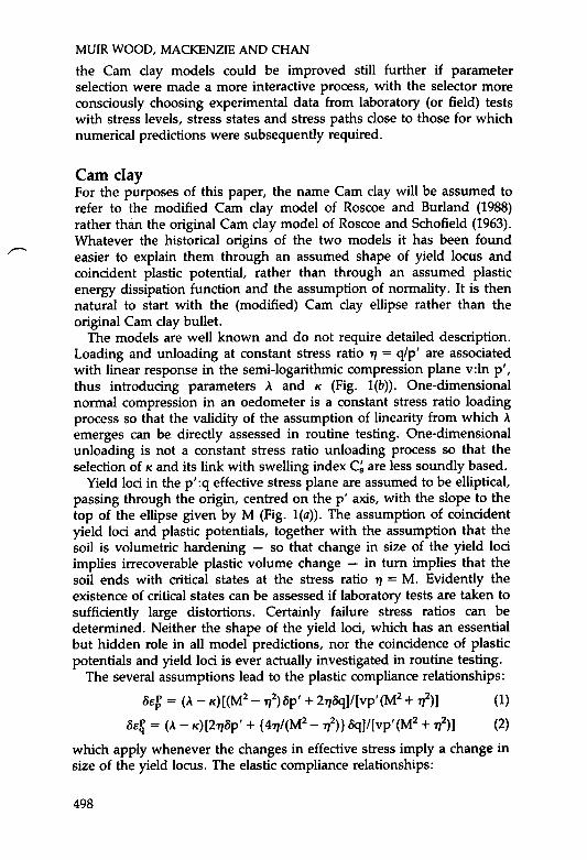
Cam clayFor the purposes of this paper, the name Cam clay will be assumed torefer to the modified Cam clay model of Roscoe and Burland (1988)rather than the original Cam clay model of Roscoe and Schofield (1963).Whatever the historical origins of the two models it has been foundeasier to explain them through an assumed shape of yield locus andcoincident plastic potential, rather than through an assumed plasticenergy dissipation function and the assumption of normality. It is thennatural to start with the (modified) Cam clay ellipse rather than theoriginal Cam clay bullet.

The models are well known and do not require detailed description.Loading and unloading at constant stress ratio 11 = q/p' are associatedwith linear response in the semi-logarithmic compression plane v:ln p',thus introducing parameters A and K (Fig. l(b)). One-dimensionalnormal compression in an oedometer is a constant stress ratio loadingprocess so that the validity of the assumption of linearity from which Aemerges can be directly assessed in routine testing. One-dimensionalunloading is not a constant stress ratio unloading process so that theselection of K and its link with swelling index C~ are less soundly based.

Yield loci in the p':q effective stress plane are assumed to be elliptical,passing through the origin, centred on the p' axis, with the slope to thetop of the ellipse given by M (Fig. l(a)). The assumption of coincidentyield loci and plastic potentials, together with the assumption that thesoil is volumetric hardening - so that change in size of the yield lociimplies irrecoverable plastic volume change - in turn implies that thesoil ends with critical states at the stress ratio 11 = M. Evidently theexistence of critical states can be assessed if laboratory tests are taken tosufficiently large distortions. Certainly failure stress ratios can bedetermined. Neither the shape of the yield loci, which has an essentialbut hidden role in all model predictions, nor the coincidence of plasticpotentials and yield loci is ever actually investigated in routine testing.

The several assumptions lead to the plastic compliance relationships:8£~ = (A - K)[(M2 - 1118p' + 211c5q]/[Vp' (M2 + 111] (1)

8£~ = (A - K)[2118p' + {411/(M2-111}c5q]/[vp'(M2+ 111] (2)

which apply whenever the changes in effective stress imply a change insize of the yield locus. The elastic compliance relationships:~

498

q

p':1 1n p'

Fig. 1.(a) Elliptical Cam clay yield locus in p':q effective stress plane;(b) isotropic compression line (iso-ncl), critical state line (csl), and unloading-reloading line (url) in v:ln p' compression plane

BE~ = [K/(Vp')] Bp'

BE~ = [1/(3G)] b'q

(3)

(4a)

orfJE~ = [2(1 + II)K]5q/[9(1- 211)vp'] (4b)

apply for all changes in effective stress. The symbols for volumetric anddistortional increments, fJEp' fJEq' are chosen following Calladine (1963)to indicate work conjugacy with the volumetric and distortional effectivestresses p/, q. .

Shear modulus G, or Poisson's ratio II, enters as a second elasticparameter, to complete the description of the isotropic elastic propertiesof the soil. It is recognised that with bulk modulus K = Vp'/K prop-ortional to mean effective stress p' it is not thermodynamically accept-able to have shear modulus also proportional to p', as is impliedthrough the selection of a constant value of Poisson's ratio v (Zytynski etal., 1978). This will in practice cause problems only when predictions arerequired of response of soils to cycles of loading and unloading.

The fifth soil parameter is required in order to be able to calculate thecurrent specific volume v from the known stress history of the soil. If thesize of the current yield locus is given by po (Fig. l(a» then:

v = r - A In (po/2pr) + K In (po/2p') (5)

where rand pr/ define a reference point on the critical state line in thecompression plane. Conventionally pr' = 1 measured in whatever unitsof stress are being used. A stress of 1 kPa is extremely low for most

499


engineering purposes. If pr'= 4 kPa then r = 1 + GsWL' indicating thelink between this reference volume r and liquid limit (Muir Wood,1990). The choice of this reference stress would not be important if thev:ln p' relationships were indeed linear over the stress range from p,( tothe stresses of engineering interest. Experimental evidence does notalways support this (Butterfield, 1979) and since the range of meaneffective stress experienced in typical geotechnical structures is not greatit might be more rational to choose the value of p,( to match the ambientmean effective stress and then choose r to fit the in situ specific volume.

Experimental dataData to be fitted with the Cam clay model are obtained from the series ofexperiments performed in the Cambridge True Triaxial Apparatus(Wood and Wroth, 1972; Airey and Wood, 1988) and described by Wood(1974). These tests were performed on samples of spestone kaolin(wp = 0.40, WL = 0.72, 73% finer than 2.um) consolidated in the TrueTriaxial Apparatus from a slurry prepared at a water content equal totwice the liquid limit. The True Triaxial Apparatus permits independentcontrol of three principal stresses (or principal strains) without allowingany rotation of principal axes. Stress paths can be continued withoutinterruption from consolidation to shearing (within the deformationcapability of the apparatus).

The (effective) stress path of test L1 is shown in Fig. 2. It consists ofanisotropic compression (1/ = 0.3) to p' = 150 kPa and unloading(DAB), followed by isotropic reloading (CDF) with two cycles ofconstant p' loading and unloading (OED) with p' = 100 kPa; FGF withp' = 150 kPa. The whole test was performed with two stresses equal toeach other (IT2 = IT3) and could in principle therefore have beenperformed in a conventional triaxial apparatus.

Proceeding incrementally, the value of A can be deduced from the

q

0

p'Fig. 2. Stress path attest U: OABCDEDFGF

500


~

50 80 100 150 kPap'

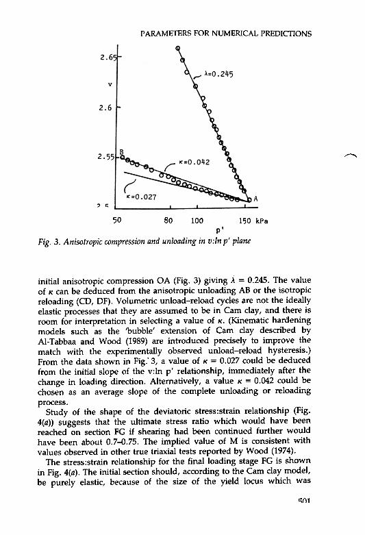
Fig. 3. Anisotropic compression and unloading in v:ln p' plane

initial anisotropic compression OA (Fig. 3) giving A = 0.245. The valueof K can be deduced from the anisotropic unloading AB or the isotropicreloading (CD, DF). Volumetric unload-reload cycles are not the ideallyelastic processes that they are assumed to be in Cam clay, and there isroom for interpretation in selecting a value of K. (Kinematic hardeningmodels such as the 'bubble' extension of Cam clay described byAl-Tabbaa and Wood (1989) are introduced precisely to improve thematch with the experimentally observed unload-reload hysteresis.)From the data shown in Fig: 3, a value of K = 0.027 could be deducedfrom the initial slope of the v:ln p' relationship, immediately after thechange in loading direction. Alternatively, a value K = 0.042 could bechosen as an average slope of the complete unloading or reloading

process.Study of the shape of the deviatoric stress:strain relationship (Fig.

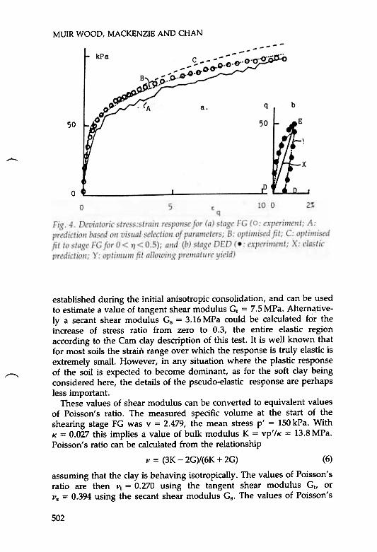
4(a» suggests that the ultimate stress ratio which would have beenreached on section FG if shearing had been continued further wouldhave been about 0.7-Q.75. The implied value of M is consistent withvalues observed in other true triaxial tests reported by Wood (1974).

The stress:strain relationship for the final loading stage FG is shownin Fig. 4(a). The initial section should, according to the Cam clay model,be purely elastic, because of the size of the yield locus which was

~m


50

~

0

~

established during the initial anisotropic consolidation, and can be usedto estimate a value of tangent shear modulus Gt = 7.5 MPa. Altem~tive-ly a secant shear modulus Gs = 3.16 MPa could be calculated for theincrease of stress ratio from zero to 0.3, the entire elastic regionaccording to the Cam clay description of this test. It is well known thatfor most soils the strain range over which the response is truly elastic isextremely small. However, in any situation where the plastic responseof the soil is expected to become dominant, as for the soft clay beingconsidered here, the details of the pseudo-elastic response are perhapsless important.

These values of shear modulus can be converted to equivalent valuesof Poisson's ratio. The ~easured specific volume at the start of theshearing stage FG was v = 2.479, the mean stress pi = 150 kPa. WithK = 0.027 this implies a value of bulk modulus K = Vp'/K = 13.8 MPa.

Poisson's ratio can be calculated from the relationshipv = (3K - 2G)/(6K + 2G) (6)

assuming that the clay is behaving isotropically. The values of Poisson'sratio are then Vt = 0.270 using the tangent shear modulus Gt, orVs = 0.394 using the secant shear modulus Gs. The values of Poisson's

502

£q

Fig. 5. Volumetric and deviatoric strain for DED (e), FG (0)

,

ratio would be reduced if hi~her values of K were used to calculatecorrespondingly lower values of bulk modulus. Rather similar values ofPoisson's ratio can be calculated from the intermediate loading cycleOED (Fig. 4(b»: the initial tangent stiffness gives GI = 5.0 MPa a~VI = 0.274, the overall secant stiffness gives Gs = 1.49 MPa andVs = 0.424. .

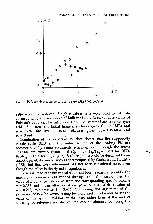
Examination of the experimental data shows that the supposedlyelastic cycle OED and the initial section of the loading FG areaccompanied by some volumetric straining, even though the stresschanges are entirely distortional (5p' = 0) (5Erl5Eq = 0.239 for OED,5Erl5Eq = 0.505 for FG) (Fig. 5). Such response could be described by ananisotropic elastic model such as that proposed by Graham and Houlsby(1983), but that extra refinement has not been considered here, eventhough the effect is clearly not insignificant.

If it is assumed that the critical state had been reached at pointG, themaximum deviator stress applied during the final shearing, then thevalue of r could be calculated from the corresponding specific volumev = 2.388 and mean effective stress p' = 150 kPa. With a value ofA = 0.245, this implies r = 3.616. Continuing the argument of theprevious section, however, it may be more useful to be able to set thevalue of the specific volume at the start rather than at the end ofshearing. A reference specific volume can be obtained by fixing the

~I)q


location of the isotropic normal compression line in the compression

plane:v = N-Alnp' (7)

According to the Cam clay model:N = r + (A - K) In 2 (8)

Combination of the specific volume and mean effective stress at F withthe known stress history, through the Cam clay model with A = 0.245,K = 0.027, M = 0.75, leads to a value of N = 3.739 (which in turnimplies, from (8), r = 3.588).

Optimisation procedureAs an alternative to direct individual estimation of values of parametersfor the Cam clay model the possibility of using an automatic optimisa-tion procedure to produce a simultaneous best fit set of parameters hasbeen explored. Such a procedure can be adapted to ensure that the fit isobtained over the range or ranges of stress change that are expected tobe relevant in a particular application - with the emphasis on the abilityto match and predict response under working loads which may not

approach failure.The stress:strain response that emerges from a constitutive model is

an extremely non-linear function of several model parameters. In only avery few cases will it be possible to obtain an analytical solution to thesearch for the optimum set of parameters, and a numerical procedure isto be preferred. The procedure adopted here is that propose.d byRosenbrock (1960), and the program used for the optimisation processhas been adapted from a program written by Klisinski (1987).

The program searches for the set of n parameters that produces theminimum value of an objective function F which is a measure of theoverall difference between experimentally observed and numericallypredicted responses. With a given starting set of parameters, theprogram varies each parameter in turn in order to discover whichdirection in n-dimensional parameter space leads to the greatest im-provement in the value of F. A new set of parameters related to the firstby the direction of maximum improvement is then chosen and theprocedure is repeated. The process is adaptive in that the direction ofmaximum improvement will in general involve variation of more thanone of the n parameters: a set of n mutually orthogonal directions ofprogressively decreasing improvement is computed and the search forfurther improvement makes use of this previously determined set of

directions.The procedure moves through n-dimensional parameter space in the

direction of greatest change of the function F, but since it retains

"nJ.

£

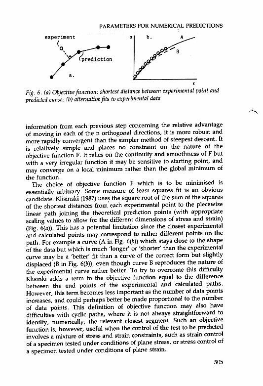
Fig. 6. (a) Objective function: shortest distance between experimental point and

predicted curve; (b) alternative fits to experimental data

'""'"'

information from each previous step concerning the relative advantageof moving in each of the n orthogonal directions, it is more robust andmore rapidly convergent than the simpler method of steepest descent. Itis relatively simple and places no constraint on the nature of theobjective function F. It relies on the continuity and smoothness of F butwith a very irregular function it may be sensitive to starting point, andmay converge on a local minimum rather than the global minimum of

the function.The choice of objective function F which is to be minimised is

essentially arbitrary. Some measure of least squares fit is an obviouscandidate. Klisinski (1987) use~ the square root of the sum of the squaresof the shortest distances from each experimental point to the piecewiselinear path joining the theoretical prediction points (with appropriatescaling values to allow for the different dimensions of stress and strain)(Fig. 6(a)). This has a potential limitation since the closest experimentaland calculated points may correspond to rather different points on thepath. For example a curve (A in Fig. 6(b)) which stays close to the shapeof the data but which is much 'longer' or 'shorter' than the experimentalcurve may be a 'better' fit than a curve of the correct form but slightlydisplaced (B in Fig. 6(b)), even though curve B reproduces the nature ofthe experimental curve rather better. To try to overcome this difficultyKlisinki adds a term to the objective function equal to the differencebetween the end points of the experimental and calculated paths.However, this term becomes less important as the number of data pointsincreases, and could perhaps better be made proportional to the numberof data points. This definition of objective function may also havedifficulties with cyclic paths, where it is not always straightforward toidentify, numerically, the relevant closest segment. Such an objectivefunction is, however, useful when the control of the test to be predictedinvolves a mixture of stress and strain constraints, such as strain controlof a specimen tested under conditions of plane stress, or stress control ofa specimen tested under conditions of plane strain.

505


It has been preferred here to define the objective function directly interms of the differences between corresponding points on the calculatedand experimental paths, using experimental values of one set ofquantities to control the prediction. For example, in stress driven pathsthe calculated path is forced to pass through all the stress points, andthe objective function is simply the sum of the squares of the straindifferences.

Both these objective functions have the disadvantage that sections ofthe path with widely spaced experimental points will receive lessweighting than sections with many points. This could be overcome byweighting each increment of the objective function by some measure ofthe distance between adjacent points on the experimental path.

The program requires a file of the experimental data points to befitted; a file containing the control path which provides input for theprediction; and a file which specifies the lower and upper bounds to then parameters, initial values of these parameters, and an indication ofwhether each parameter is allowed to be varied as part of the

optimisation procedure.The Cam clay model is most conveniently described in terms of the

strain response to changes in effective stress. The model is complete inthe sense that it is able to make predictions of response in all regions ofstrain space - including independent variation of all three principalstrains, rotation of all three principal axes. However, the structure of themodel implies that not all changes in stress are permissible. Any attemptto cause plastic deformations with stress ratio 1] > M leads to collapse ofthe yield surface: the soil cannot support outward stress increments,and a section of stress space (which depends on the current size of theyield surface) is thus inaccessible. It is therefore preferable to use as thecontrol path the observed strain path even where, as for the true triaxialtests used here, the test has been conceived as a stress-controlled test,because while every strain increment implies a corresponding stressincrement the converse is not always true.

ResultsAlthough the primary objective is to improve the prediction of themodel during the shear stage FG, it is of interest to observe how theoptirnisation procedure attempts to cope with other stages of the test.The volumetric data (specific volume and mean effective stress) from theinitial anisotropic consolidation OA have been used to obtain a value forA = 0.245. The optimisation program prefers a slightly higher valueA = 0.272, partly because the definition of objective function F implicitlygives greater weight to the data at higher stresses. The optirnisationprocedure for this stage can also present an opinion on the values of theother parameters because these control the link between stress ratio 1/

506

,, ,


and ratio of distortional to volumetric strain Se./Sep. Cam clay is notvery good at getting this link correct: Muir Wood (1990) notes that Camclay tends to predict values of earth pressure coefficient at rest Ko which

lie above Jaky's (1948) empirical expressionKo = 1 - sin 4>' (9)

unless simultaneous low values of both JI and A = (A - K)/A areassumed, implying dominance of the deformation by low Poisson's ratioelastic response. The optimisation program suggests JI = 0.37 butK = 0.26, implying A = 0.04, and M = 0.86.

The procedure can also be applied to the anisotropic unloading stage.The average value of K = 0.04 for this stage is confirmed, but there is aproblem with the search for the optimum value of JI (the only otherparameter which has any effect during this elastic unloading). A verysmall positive shear strain was observed during unloading, while thedeviator stress q was reducing. This pattern of response cannot bepredicted with an isotropic elastic model. The best the program can do isto set JI = 0.5, making the shear modulus as low as possible, so that thepredicted stress path shows no change in q.

The cycle of loading and unloading OED, with p' = 100 kPa, isexpected to be purely elastic according to Cam clay, with the knownstress history. The observed, typically hysteretic, shape of the stress -strain response on this cycle (Fig. 4(b» clearly conflicts with thisexpectation, and theprogram,c not surprisingly, is not particularly happyin trying to fit the data varying only G, or K and JI. (Although this is apurely distortional stress path, both K and JI are required in order tocompute the value of the shear modulus.) The objective function F inthis case seems to be rather flat and undulating (a Cambridge-likelandscape) with a number of false minima: convergences are obtainedwith JI = 0.12, K = 0.15 but also with JI = 0, K = 0.34 (Fig. 4(b): line X).

With M = 0.75, the size of the yield locus created by the originalconsolidation OA is po = 174 kPa. If this known history is ignored thenthe observed behaviour on cycle OED can be better matched with anelastic-plastic Cam clay prediction with po = 130 kPa, and withG = 3.25 MPa, K = 0.20, A = 0.26, M = 0.68 (Fig. 4(b): curve Y). This isa more robust minimum to which the optimisation process is able toconverge from several different starting points. Whether such a distor-tion of the actual history would be acceptable from an engineering pointof view is a separate issue. Besides, the value of shear modulus that hasbeen selected implies a negative value of Poisson's ratio.

The final shearing FG is best fitted with the set of parametersG = 4.09 MPa, K = 0.35, A = 0.62, M = 0.82 (Fig. 4(a): curve B). Theoptimisation procedure is happy to choose the size of the yield locus atthe start of shearing to be po = 178 kPa, which is surprisingly but

507

MUIR WOOD, MACKENZIE AND CHANgratifyingly close to the value po = 170 kPa calculated from the knownhistory with M = 0.82. This is again a rather robustly convergent set ofparameters. It might be suggested that the value M = 0.82 gives a truerestimate of the stress ratio towards which the stress:strain response isactually heading. Again the chosen combination of shear modulus and Kimplies a negative value of Poisson's ratio. If it is required to restrict thesearch to 11>0 then the optimum fit is obtained with 11=0.0, K = 0.18,A = 0.45, M = 0.82. It is significant that the value of (A - K) has

remained almost the same, while the individual values have changed: itis (A - K) that primarily controls the magnitude of the plastic distortionalstrain increments 5eqP (eqn. (2». It is particularly the value of A = 1 -KIA that is being pulled down, indicating that improved fitting isobtained by increasing the contribution of the recoverable component ofvolumetric deformation. A zero or negative value of Poisson's ratio,implying a low ratio K/G

K/G = (2/3)(1 + 11)/(1 - 211) (10)

is also apparently beneficial, but the present Cam clay algorithm doesnot permit negative Poisson's ratio to be specified.

However, if the optimisation procedure is applied only to the initialpart of the shearing FG, up to stress ratio 1/ = 0.5, then the optimum fit

IiOR


is obtained with G = 5.0 MPa, K = 0.43, A = 0.58, M = 0.78 andpo = 172 kPa (Fig. 4(a): curve C) (or 1/ = 0.0, K = 0.13, A = 0.28,M = 0.80, again with the same difference (A - K) being chosen) - butthese sets of parameters give a worse overall fit to the data of the wholeshearing ~tage. Clearly the choice of parameters can be tuned to matchthe data over a selected range of interest. Both curves Band C in Fig.4(a) provide a major improvement over the prediction based on thevisual, stepwise selection of parameters (curve A).

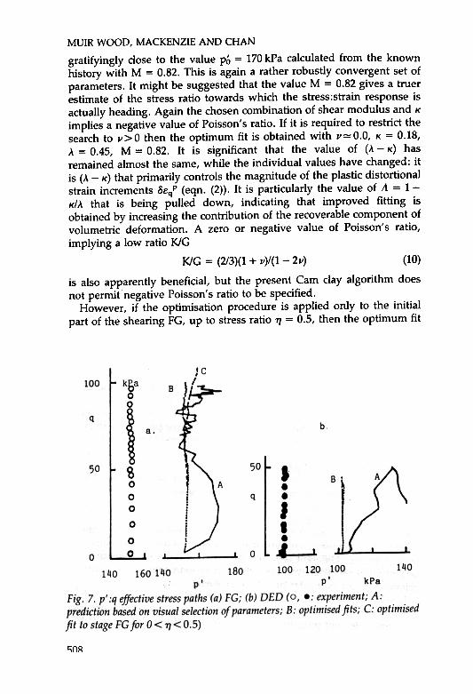
The volumetric response has not been mentioned so far. The strainpath is used as input to control the prediction; the success of thevolumetric response can be judged by comparing the predicted stresspaths with the (applied) constant mean stress paths (Fig. 7(a), (b». Indetail these paths are of course very sensitive to erratic changes indirection of the (experimentally derived) strain paths, particularly withthe visual stepwise selected parameters (curves A). The optimisationprocedure is very successful in matching the actual stress changes

(curves B).

'"""

Discussion and conclusionsThe stress path method (Lambe, 1967) seeks to encourage engineers tomatch laboratory and field stress paths in order to be able to estimatefield deformations in a more rational way. Estimation of field deforma-tions is more readily achieved by numerical analysis than by handcalculation, and consideration of stress paths encourages engineers to beaware of the nature of the extrapolation that is implied in the numericalpredictions (Wood, 1984). It is a logical extension then to encourageengineers to make their numerical models match the experimental dataover the ranges of stress or strain changes that are actually expected tobe important. Clearly this will often be an iterative process, with stresspaths that emerge from numerical analyses performed for working loadsbeing used to define the range of stress in laboratory tests over whichthe optimum set of soil parameters should be assessed.

The possibilities of optimisation in parameter selection have beenpresented here for just one test, to illustrate some of the problems thatmay emerge. It would normally be preferable to combine data fromseveral tests, either repeating the response on a single path, to providesome information about reliability of experimental data, or in order toincrease the volume of relevant stress hyperspace over which data havebeen gathered. Different tests can be assigned different weights in theoptimisation procedure in order to reflect assessments of test quality or

relevance to the particular prototype problem.It will be noted that no suggested optimum values of r or N have

been quoted. The Cam clay algorithm used here is typical of those usedwith finite element programs (see, for example, Britto and Gunn (1987»

509


in that it expects the initial size POi of the yield surface to be specified atthe same time as the initial effective stresses. The initial specific volumeVi is required in order that strain increments may be calculated from(IH4) but the link between Vi, POi and initial mean effective stress pithrough N, A and K is not forced:

Vi = N - A In POi + K In (pOi/p') (11)

the value of POi becomes an optimisation variable, whereas comparisonand combination of tests with different consolidation histories requiresthat N or r be used instead. This merely requires a minor programmodification.

It would of course be quite unwise to use such an optimisationprocedure without interaction with an informed user. The processcannot be allowed to become a 'black box'. The user needs to ensure thatthe parameters that are chosen are indeed reasonable, and needs to beintelligent in choosing data which cover the appropriate stress level andstress and strain ranges. The objective function for a model like Camclay has many minima, and it is clearly sensible to seed the optimisationprocess with initial values which have been deduced from visualinterpretation of the experimental observations in the traditionalmanner.

Nevertheless, releasing the Cam clay parameters from their physicalorigins, and concentrating the prediction on stress changes of prototypeinterest, improves the performance of the model. It remains a simplemodel, requiring a small number of soil parameters, and it may bepreferable to tune it to give a good local prediction of response, ratherthan to tune it to the global responSe of the soil and still to expect it toperform well locally.

AcknowledgementsSome of the work described here was performed by the second authorwith support from the Science and Engineering Research Council undergrant GR/E84167.

ReferencesAIREY, D.W. AND WOOD, D.M. (1988). The Cambridge true triaxial

apparatus. In Advanced triaxial testing of soil and rock (eds. R. T.Donaghe, R.C. Chaney and M.L. Silver) ASTM, STP977, pp. 796-805.

AL-TABBAA, A. AND WOOD, D.M. (1989). An experimentally based'bubble' model for clay. Numerical models in geomechanics NUMOGIII (eds. S. Pietruszczak and G.N. Pande) Elsevier Applied Science,pp. 91-99.

510

""'


BRITfO, A.M. AND GUNN, M.J. (1987). Critical state soil mechanics viafinite elements. Ellis Horwood.

BUTfERFIELD, R. (1979). A natural compression law for soils (an advanceon e-iog pi). Geotechnique, Vol. 29, No.4, pp. 469-480.

CALLADINE, C.R. (1963). The yielding of clay. Geotechnique, Vol. 13, No.3, pp. 250-255.

GRAHAM, J. AND HOULSBY, G.T. (1983). Elastic anisotropy of a naturalclay. Geotechnique, Vol. 33, No.2, pp. 165-180.

JAKY, J. (1948). Pressure in silos. Proc. 2nd ICSMFE, Rotterdam Vol. 1,pp. 103-107.

KLISINSKI, M. (1987). Optimisation program for identification of constitu-tive parameters. Structural Research Series No. 8707, Department ofCivil, Environmental, and Architectural Engineering, University ofColorado, Boulder.

LAMBE, T.W. (1967). Stress path method. Proc. ASCE, Vol. 93, SM6, pp.309-331.

MOURATIDIS, A. AND MAGNAN, J.-P. (1983). Modele elastoplastiqueanisotrope avec ecrouissage pour Ie calcul des ouvrages sur solscompressibles. Rapport de recherche, Laboratoires des Ponts etChaussees No. 121.

MUIR WOOD, D. (1990). Soil behaviour and critical state soil mechanics.Cambridge University Press.

ROSCOE, K.H. AND BURLAND, J.B. (1968). On the generalised stress-strainbehaviour of 'wet' clay, in Engineering plasticity (eds. J. Heyman andF.A. Leckie) Cambridge University Press, pp. 535-609.

ROSCOE, K.H. AND SCHOFIELD, A.N. (1963). Mechanical behaviour of anidealised 'wet' clay. Proc. 2nd Eur. Conf. SMFE, Wiesbaden 1, pp.47-54.

ROSENBROCK, H.H. (1960). An automatic method for finding the greatestor least value of a function. The Computer Journal, Vol. 3, pp.

175-184.SCHOFIELD, A.N. AND WROTH, C.P. (1968). Critical state soil mechanics.

McGraw-Hill.WOOD, D.M. (1974). Some aspects of the mechanical behaviour of kaolin

under truly triaxial conditions of stress and strain. PhD thesis,

Cambridge University.WOOD, D.M. (1984). Choice of models for geotechnical predictions. In

Mechanics of engineering materials (eds. C.S. Desai and R.H. Gal-lagher) John Wiley, pp. 633-654.

WOOD, D.M. AND WROTH, C.P. (1972). Truly triaxial shear testing of soilsat Cambridge. Proc. Int. Symp., The deformation and the rupture ofsolids subjected to multiaxial stresses, Cannes, RILEM Vol. 2, pp.

191-205.WROTH, C.P. (1977). The predicted performance of a soft clay under a~

1;11

/"""-,


trial embankment loading based on the Cam clay model. Finiteelements in geomechanics (ed. G. Gudehus) J. Wiley, pp. 191-208.

WROTH, C.P. AND WOOD, D.M. (1975). Critical state soil mechanics.Lecture notes for short course given at Chalmers Tekniska H6gskola,

G6teborg.WROTH, C.P., WOOD, D.M. AND HOULSBY, G.T. (1981). Critical state soil

mechanics. Lecture notes for short course given at Oxford University.WROTH, C.P., WOOD, D.M. AND HOULSBY, G.T. (1985). Critical state soil

mechanics. Lecture notes for short course given at CambridgeUniversity .

WROTH, C.P., WOOD, D.M., HOULSBY, G.T. AND BROWN, S.F. (1982).Critical state soil mechanics. Lecture notes for short course given at

Nottingham University.WROTH, C.P., WOOD, D.M. AND STEENFELT, J. (1979). Critical state soil

mechanics. Lecture notes for short course given to Dansk Geoteknisk

Forening, Lyngby.ZYTYNSKI, M., RANDOLPH, M.F., NOVA, R. AND WROTH, C.P. (1978). On

modelling the unloading-reloading behaviour of soils. Int. J. forNumerical and Analytical Methods in Geomechanics, Vol. 2, pp.87-94.

512

year of publication:- of parameters for numerical... · muir wood, mackenzie and chan the cam clay...

Documents