1

YEDITEPE UNIVERSITY

DEPARTMENT OF ELECTRICAL AND ELECTRONICS ENGINEERING

EE323 ELECTROMAGNETIC WAVES AND TRANSMISSION LINES LABORATORY

2015-2016 SPRING

EXPERIMENT 1

CHAPTER 1: INTRODUCTION TO MATLAB INTRODUCTION: MATLAB, whose name is an acronym for “MATRIX LABORATORY”, is a high level language and interactive environment for numerical computation, visualization and programming. In many areas including communications, signal processing, image and video processing, control systems, finance, where high level mathematics and programming with numerical analysis is needed, MATLAB is a powerful tool for problem definition, solving and optimization. Since the electromagnetic theory includes the operations of advanced calculus, MATLAB will be a guiding tool for understanding the outcomes of the various phenomena, by demonstrating the visual outputs with different monitoring tools.

2

WORKING WITH MATLAB: VARIABLE DEFINITION When you double-click the MATLAB icon, a new MATLAB window is opened.

Figure 1. MATLAB WINDOW

As seen in Figure 1, you can create new variables using Command Window and see the defined-variable-list in the “Workspace” Tab. Also, you can create your own folder and define it as the current folder for saving the script files. The “Current folder tab on the left of the window, shows the previously-created MATLAB files’ list.

SAY HELLO TO MATLAB In all programming courses, first thing is printing a word into the screen. This is a

very first action when beginning in every programming software. To say “Hello” or something to MATLAB and see the output, you can use “disp()” function, defined in MATLAB. Just as an example to say “Hello”, write the following command: >> disp('HELLO MATLAB, THIS IS MY FIRST SENTENCE!!');

DEFINE A SCALAR VARIABLE For defining a variable, just write the equation. For example, if you create a variable named “x” which is equal to 5, just write the following command and press ENTER: >> x=5

3

If you place a semicolon at the end of the equation, you do not see MATLAB output but still, your variable is created. You can see the difference between putting and not putting a semicolon at the end of the command in figure 2. In most of the applications, your variable may have more than 1 value. When the definition is completed, you can fill the screen with values of your variable. To prevent that, always put a semicolon at the end of each command.

Figure 2. Difference between putting and not putting a semicolon.

DEFINING AN EXPONENTIAL VARIABLE WITH BASE “10”

In electromagnetism, one may need to define some constants which are exponential numbers with base 10. To do that, the letter “e” may be used. To show an example

which defines MHzf 1 , 7

0 10.4 and 9

0 10.36

1

:

>> f=1e6

uo=(1e-7)*4*pi

eo=(1e-9)*(1/(36*pi))

f =

1000000

uo =

1.2566e-006

eo =

8.8419e-012

DEFINE A VECTORIAL VARIABLE

In most of the applications, your variable may have values more than 1. For example, you have a circuit to be tested and you have made measurements at each second for 1-minute-duration. This means that your “time variable” has 60 values which are “1,2,3…60” To define a such a variable in MATLAB, you can use the following command in figure 3:

4

Figure 3. Definition of an array with initial, final and increment values

Also, a vectorial variable may be defined with “linspace( )”function. Following example, creates a variable named “t” from 1 to 60 @ 50 points: >> t=linspace(1,60,50)

In this example, your variable has regularly-spaced elements. But what if you want to define a variable which has elements with unregularly-spaced? Suppose that you have variable which has 5 elements whose values are: -2, 3.42, 5.819, 0, -0.01. To define such a variable called “y”, you may write the following command: >> y=[-2 3.42 5.819 0 -0.01];

When you write this command, you actually create a 1x5 matrix which has one row and five columns. If you want to define the same variable in 5x1 matrix form you can define the same variable by typing: >> y=[-2; 3.42; 5.819; 0; -0.01];

If you want to create such a matrix

9811

004.1022514

600

181.374.2

A

Just write the following command: >> A= [2.74 3.81 1;0 0 6;14 225 10.004;1 1 98];

You can also create vectors defined in Cartesian coordinate systems. Suppose that you

have a vector which is defined as: kjıA ˆ5ˆ2ˆ3 . You can define the same vector in

MATLAB by writing following command: >> A= [3 2 5];

This vector indicates that, it has x-component whose magnitude is 3, y-component whose magnitude is 2 and z-component whose magnitude is 5. As you will remember

from Mathematics, the total length of the vector can be found as: 38523 222 .

To find the same result in MATLAB, the following command is used:

5

>> norm(A)

ans =

6.1644

Also, you can find a unit vector in the direction of the vector “A”. As you remember from vector calculus, (sure you all remember!!) a vector has a magnitude and direction as shown in figure 4. You can find the unit vector whose direction is the same as the

original vector, by dividing the vector by its magnitude. To show algebraically:S

Ss

ˆ To

calculate the unit vector of the previous example in MATLAB, you can write the following code: >> A=[3 2 5];

>> unit_vector=A/(norm(A))

unit_vector =

0.4867 0.3244 0.8111

Figure 4.Vector Components in Cartesian Coordinate System

ARITHMETIC OPERATIONS

o ADDING (+) / SUBTRACTING (-) You can sum or subtract 2 variables simply by using “+” or “-“sign. To give an example: >> x=3;

>> y=10;

>> z=x+y

z =

13

In some cases, your variables may be vectors. In this situation, you may have to perform summation or subtraction operation with one vectorial and one scalar variable. To give an example:

6

>> x=10;

>> y= [1 2 3];

>> z=x-y

z =

9 8 7

As you see, if you perform subtraction operation with one vector and one scalar, all elements inside the vector is subtracted from scalar variable. If you perform a summation/subtraction operation between 2 vectors, you must be aware of the fact that, their sizes must be equal. This means that you cannot add 4-element vector to 3-element vector. >> W= [1 2 3];

>> y= [4 5 6];

>> z=W+y

z =

5 7 9

>> A= [7 5 3];

>> B= [1 5 9 7];

>> C=A+B

??? Error using ==> plus

Matrix dimensions must agree.

o MULTIPLICATION/DIVISION (SCALAR*VECTORIAL)

As we know from the mathematics, if vector is multiplied/divided by a scalar, all elements inside the vector is multiplied/divided by with that scalar. To show it in MATLAB, you can create a scalar and a vector and multiply them!

>> A=10;

>> B= [-2 5.1 8.78 10 9];

>> C=A*B

C =

-20 51 87.8 100 90

>> D=B/A

D =

-0.2 0.51 0.878 1 0.9

7

o MULTIPLICATION/DIVISION (VECTORIAL*VECTORIAL) In some cases you may want to perform vectorial multiplication/division operation. In this case, vector sizes must be equal. Otherwise you cannot perform element-by-element multiplication. An element-by-element multiplication can be showed as follows:

nnnn BA

BA

BA

B

B

B

A

A

A

22

11

2

1

2

1

It must be noted that, A and B vectors should have the same size. To perform this multiplication in MATLAB you can use following command: >> A= [2 6 4 8 7 9];

>> B= [3 2 1 5 9 7];

>> C=A.*B

C =

6 12 4 40 63 63

Note that the multiplication procedure is the same. But you have to put a “.” next to the first vector.

o SCALAR (DOT) PRODUCT OF 2 VECTORS In Cartesian coordinate system, there are 3 coordinates “x”, “y” and “z”. The corresponding unit vectors for these coordinates are defined as “i”, “j” and “k” respectively. Generally, a vector may have 3 components in Cartesian coordinate system and may be represented as:

kAjAıAA zyxˆ.ˆ.ˆ. .

Scalar (Dot) product of two vectors is defined as the summation of 3 elements, obtained by the multiplication of 2 elements in the same coordinate vector. To show algebraically;

zzyyxx

zyxzyx

BABABABA

kBjBıBkAjAıABA

kjkıjı

kkjjıı

ˆ.ˆ.ˆ.ˆ.ˆ.ˆ.

0ˆˆˆˆˆˆ

1ˆˆˆˆˆˆ

8

Do not forget the fact that dot product of 2 vectors is SCALAR!! You can use MATLAB to calculate dot product of 2 vectors. To show in an

example:

o VECTOR (CROSS) PRODUCT The cross product of two vectors is defined as another vector, perpendicular to the plane containing those two multiplicative vectors as shown in figure 5. To make the definition more clear, algebraic definition can be shown.

Figure 5. Cross-Product of Two vectors

Let the unit vectors in Cartesian coordinate system (x-y-z) be “ kjı ˆ,ˆ,ˆ ”

respectively. Definition of cross product in unit vectors can be written as:

jkıjık

ıjkıkj

kıjkjı

kkjjıı

ˆˆˆˆˆˆ

ˆˆˆˆˆˆ

ˆˆˆˆˆˆ

0ˆˆˆˆˆˆ

Using these relations between unit vectors, cross product of two vectors in Cartesian coordinate system can be shown as:

zyx

zyx

xyyxzxxzyzzy

zyxzyx

BBB

AAA

kjı

BABAkBABAjBABAı

kBjBıBkAjAıABA

ˆˆˆ

ˆˆˆ

ˆˆˆˆˆˆ

,

9

To evaluate the cross product of 2 vectors in MATLAB, you can use “cross()” function. To show in an example: >> A=[5 8 7];

>> B=[1 3 2];

>> cross(A,B)

ans =

-5 -3 7

Note that the resulting vector whose coordinates are “-5”, “-3” and “7” is perpendicular to both A and B since the cross-product operation of two vectors creates a vector perpendicular to both vectors.

THE FOR LOOP In the for loop, you must define where to start and stop. Basically, give a vector in the "for" statement and MATLAB will loop through for each value in the vector. In the below example, the j variable will have three values in the loop.

>> for j=1:3

j

end

This code creates the following output.

j =

1

j =

2

j =

3

SOME USEFUL FUNCTIONS size: Returns the two-element row vector containing the number of rows and columns. length: Returns the number of elements along the largest dimension of an array. max: Returns the largest element of an array. min: Returns the smallest element of an array. sum: Returns sums along different dimensions of an array. mean: Returns the mean values of the elements along different dimensions of an array. abs: Returns absolute value and complex magnitude.

exp: Returns the exponential, xe sqrt: Returns the square-root.

zeros (m,n): Returns an MxN matrix, whose elements are filled with “0”.

10

CHAPTER 2:

GRADIENT, DIVERGENCE AND CURL OPERATIONS WITH MATLAB APPLICATIONS

INTRODUCTION:

In electromagnetics, there are some quantities that depend on both time and position. To work with these quantities, there are some differential operations that will be frequently encountered in the journey of electromagnetic theory.

In this experiment, three differential operations which are “Gradient”, “Divergence”

and “Curl” will be introduced in Cartesian coordinates. These operators are still valid in any other orthogonal coordinate system such as cylindrical or spherical coordinate systems. But for simplicity of understanding the basic idea of these operators, Cartesian coordinate system will be used.

GRADIENT OF A SCALAR FIELD Gradient of a scalar field is defined as the vector that represents both the magnitude and the direction of the maximum space rate of increase. To show mathematically;

dn

dFaFgrad n

(1)

To define the operator “grad” in a more brief way, a new symbol called “del” ( ) is introduced. After rearranging, equation (1) turns into:

dn

dFaF n

(2)

If the equation (2) is shown in Cartesian coordinates, the result is the following:

z

Fa

y

Fa

x

FaF zyx

ˆˆˆ (3)

In order to explain the physical meaning of gradient, temperature-in-a-room-example can be given. Suppose that you have proper equipment to measure the temperature at various locations in a room. From this data, it is possible to connect the points which have the same temperature values. These connected-points may give necessary information about the magnitude and direction where the most rapid changes occur. To visualize that phenomenon, such an example, built in MATLAB can be given:

11

>> v = -3:0.2:3;

[x,y] = meshgrid(v);

z = 3.*x-x.^3-3.*x.*y.^2;

[px,py] = gradient(z,0.2,0.2);

subplot(1,2,1)

contour(v,v,z,20,'Linewidth',3);

hold on;

quiver(v,v,px,py,'Linewidth',2,'color','black');

hold off

xlabel('x');

ylabel('y');

title('contour plots of 3x-x^3-3xy^2');

subplot(1,2,2)

surf(z)

xlabel('x');

ylabel('y');

title('Surface plot of of 3x-x^3-3xy^2');

When you execute the script above, gradient vectors of 23 33 xyxxz can be seen in

figure 6a. Considering the arrows that show the direction of increase, the characteristics of the function is shown in figure 6b.

(a) (b)

Figure 6. a) Contour and gradient plot b) Surface plot of the function 23 33 xyxxz

12

DIVERGENCE OF A VECTOR FIELD In vector field analysis, a proper way of representing the variations of the field is using directed field lines. These lines are called flux lines. As shown in figure 7, these lines are directed lines which show the direction and magnitude of the vector field. The vector field strength is measured by the number of flux lines passing through a unit surface, normal to the vector. When an arbitrarily chosen volume with a closed surface is concerned, net flux through may be positive, negative or zero. If the net flux is positive, then the volume contains a source. If the net flux is negative, then there is a sink inside the volume. If the inward flow of the vector field is equal to outward flow, that is, the net flux through the surface is zero; the volume does not contain neither sink nor source. If there is an enclosed source in a volume, the net outward flow of the fluid per unit volume is a measure of the strength of the enclosed volume. In summary, divergence of a vector field “A” at a point is the net outward flux of A per unit volume, as the volume about the point tends to zero. To show mathematically;

v

dsAA S

v

0lim (4)

After a straightforward analysis, divergence of a vector in Cartesian coordinate system is defined as:

z

A

y

A

x

AA zyx

(5)

To calculate the divergence of a vector field, MATLAB can be used. Here is an example showing how to evaluate the divergence of a

vector field z

zyx

y

zyx

x

zyx aezaeyaexA ......222222222222 :

13

>> v=-2:0.2:2;

[x,y,z]=meshgrid(v);

fx=x.*(exp(-x.^2-y.^2-z.^2)).^2;

fy=y.*(exp(-x.^2-y.^2-z.^2)).^2;

fz=z.*(exp(-x.^2-y.^2-z.^2)).^2;

div=divergence(x,y,z,fx,fy,fz);

subplot(1,2,1)

quiver3(x,y,z,fx,fy,fz,'color','blue');

title('Arrow representation of vector field A')

xlabel('x')

ylabel('y')

zlabel('z')

subplot(1,2,2);

quiver3(x,y,z,fx,fy,fz,'color','red');

hold on

for i=1:round(length(x)/5):length(x)

surf(x(:,:,i),y(:,:,i),z(:,:,i),div(:,:,i))

end

Figure7. Vector Field “A” (shown in arrows) and its scalar divergence.

14

DIVERGENCE THEOREM (GAUSS’S THEOREM)

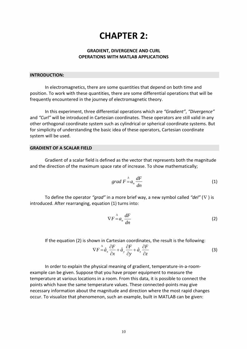
By using the definition of divergence, a very useful relation called divergence theorem can be obtained. Since the divergence of a vector field defined as the net flux per unit volume, if we integrate the divergence of the field over a volume, what we obtain is the total flux through the surface that bounds the volume. To show mathematically;

SV

dsAdvA . (6)

To describe this theorem in physical world, we can divide a closed-surfaced-volume

into small cubes. Since the whole geometry is under the effect of a vector field, all sub-geometry parts (cubes) are also under the effect of the same vector field. If we apply the scalar multiplication (dot-product) of vector field into the surface normal of each cube, some quantities will cancel each other as shown in figure 7.(green-red and pink-blue). The remaining terms are the sum of scalar multiplication of vector fields into the outer surface normal of each cube.

Figure7. Surface normal of each sub-geometry parts (cube).

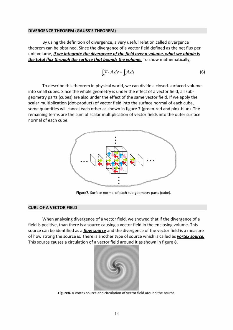
CURL OF A VECTOR FIELD When analysing divergence of a vector field, we showed that if the divergence of a field is positive, than there is a source causing a vector field in the enclosing volume. This source can be identified as a flow source and the divergence of the vector field is a measure of how strong the source is. There is another type of source which is called as vortex source. This source causes a circulation of a vector field around it as shown in figure 8.

Figure8. A vortex source and circulation of vector field around the source.

15

If a vortex source is stronger than the other, net circulation around the stronger source, will be much greater than the weaker source. So we need a quantity that defines the strength of a vortex source. So the curl of a vector field is defined as the net circulation per unit area as the area tends to zero. To show mathematically;

s

dlAAAcurl C

s

0lim (7)

After a straightforward analysis, curl of a vector field A is defined in Cartesian

coordinate system as:

zyx

zyx

AAA

zyx

aaa

A

y

A

x

Aa

x

A

z

Aa

z

A

y

Aa xy

zzx

y

yzx (8)

To calculate the curl of a vector field, MATLAB can be used. Here is an example,

showing how to evaluate the curl of vector field zyx aaxayA 0

:

v=-2:0.8:2;

[x,y,z]=meshgrid(v);

fx=-y; fy=x; fz=0.*z;

[curlx,curly,curlz]=curl(x,y,z,fx,fy,fz);

subplot(1,2,1)

quiver3(x,y,z,fx,fy,fz,'color','blue');

title('Arrow representation of vector field A')

xlabel('x')

ylabel('y')

zlabel('z')

subplot(1,2,2)

quiver3(x,y,z,fx,fy,fz,'color','blue');

hold on;

quiver3(x,y,z,curlx,curly,curlz,'color','green')

title('Arrow rep. of vector field A (blue) and its curl(green)')

xlabel('x')

ylabel('y')

zlabel('z')

When you execute the following command, what you see is the vector field in x-y-z coordinates (blue lines) and evaluation of curl operation at different points (green lines)

16

Figure8. Vector field “A” and its curl

STOKE’S THEOREM By using the definition of curl, another very useful theorem can be obtained. Since the curl of vector field is defined as the net circulation per unit area, if we integrate the curl of a vector field over an open surface, the result is the line integral of the vector along the contour, bounding the surface. To show mathematically;

CS

dlAdsA (9)

To describe this problem in physical world, we can divide a pot (“testi” in Turkish) into sub-areas, each one having an area of s . If we sum all the vectors (red ones), some of will cancel each other and the result is the sum of the vectors that covers the open edge of the pot as shown in figure 9.

Figure9. Subdivided area for proof of Stoke’s Theorem.

17

HOMEWORK: 1. Using the examples given above, evaluate the functions and their gradient, divergence

and curl operations respectively.

GRADIENT

o )( 22 yxez

o )( 22

. yxexz

o 22.yxz

DIVERGENCE

o zyx ayxayazxA .2... 22

o zyx azayaxA ...3

o zyx axzazyayxA .... 222

CURL

o zyx ayzazxyayA .2.2. 22

o zyx azxayzayxA ....

o zyx azxayzayxA .... 222

2. Using the definitions of vector operators in Cartesian system above, prove the following 2 null-identities (analytically) for any vector field “ A ”:

0 A curl of the gradient of any scalar field is zero.

0 A divergence of the curl of any vector field is zero.

3. Prove the 2 null identities using MATLAB. You can select the field functions used in the

examples.

4. The characteristic impedance of a medium is defined as the ratio of Electric field and Magnetic Field propagating in that media as shown in the equation below.

zH

zE

0

0 . Now suppose that you have the data of measured values of Electric Field

and Magnetic field in 15 different measurement setups. The resulting values are in the following table:

18

Find the average value of impedance.

5. You are given three vectors;

kjiC

kjiB

kjiA

ˆ4ˆ3ˆ

ˆ2ˆˆ2

ˆˆ2ˆ

Please find the volume of the parallelepiped, formed by three vectors A, B and C by using MATLAB. Write the corresponding code.