yield curves and international equity returns i. introduction many researchers have investigated the...

Yield Curves and International Equity Returns

James Ross McCownFlorida Atlantic UniversityJohn D. MacArthur Campus5353 Parkside DriveJupiter, FL 33458

Phone: (561)-799-8626Fax: (561)-799-8535Email: [email protected]

Version: 12/5/99

JEL codes: E43, E44, G15Keywords: International asset pricing

Abstract:

This paper examines empirical evidence on the international transmission ofshocks to financial asset markets. The relationships between yield curves and riskpremiums of stocks for eight industrialized countries are examined. Only the stocks of thethree largest economies: Germany, Japan, and the USA, show negative risk premiumsduring periods preceded by the inverted yield curves of their respective governmentbonds. This is not the case for stocks of the five smaller countries in the sample.However, four of the five smaller countries have negative risk premiums in periodspreceded by inverted German or US yield curves. This is consistent with the view that aworld risk factor, captured by major country yield curves, affects the pricing of assets insmaller economies.

The consumption CAPM is unable to explain the phenomenon of the negative riskpremiums. In almost all cases the conditional covariance between consumption growthand the risk premiums is statistically indifferent from zero.

_______________________________________________________________________I am grateful to Stephen Cecchetti, Carmelo Giacotto, Patrick Fitzgerald, Dan McCarty,Huston McCulloch, Masao Ogaki, Tim Opler, Alan Viard, and two anonymous refereesfor helpful suggestions. I also thank seminar participants at the Midwest FinanceAssociation and Southern Finance Association meetings. John Campbell and BarbaraOstdiek provided the MSCI stock return data. Masao Ogaki provided computer programsfor some of the statistical tests. Any errors are my own.

2

I. Introduction

Many researchers have investigated the relation between yield curves and

financial asset returns. Fama and French (1989), show that excess returns on US stocks

and corporate bonds are positively related to the slope of the yield curve of US Treasury

securities. Fama and French say that the yield curve has predictive ability because it is a

proxy for discount rate shocks. Both stocks and long-term Treasury bonds are long-term

investments, and are highly susceptible to changes in investors’ intertemporal discount

rates. Boudoukh, Richardson, and Smith (1993) and Ostdiek (1998) show how ex ante

risk premiums on US stocks and the world stock portfolio are negative in periods

preceded by inverted yield curves. For individual foreign countries, the research has been

limited, although Asprem (1989) examined the relationship between the US term spread

and the returns on stocks of ten European countries.

The purpose of this research is to look at the effects of foreign country yield

curves on the risk premiums of their own stocks, and also the effects of the larger

economies’ yield curves (U.S., Germany, and Japan) on the smaller countries’ stocks.

Using returns on country stock indices compiled by MSCI, these relations are tested for

eight industrialized countries, including the United States, for the period from 1970 to

1994. There is strong evidence for negative risk premiums for only the US, Germany, and

Japan, when using each country’s own yield curve. However, negative risk premiums

occur for many of the smaller economies when the US or German yield curve is inverted.

The Japanese yield curve does not show this relation with the other countries’ stocks.

This is consistent with the view that a world risk factor, captured by the US and German

yield curves, affects the pricing of assets in smaller economies.

3

Boudoukh, Richardson, and Whitelaw (1997) find that the relation between the

U.S. term spread and the risk premium on U.S. stocks is nonlinear. This research also

finds that the relation for the U.S. variables is nonlinear, but does not find the evidence to

be so strong for the other seven countries’ term spreads and stocks. However, there is a

nonlinear relation between the U.S. term spread and the risk premiums of the other seven

countries’ stocks, in particular for Canada and the UK.

The large differences of the conditional risk premiums signaled by upward-

sloping and inverted yield curves may be due at least in part to differences in the volatility

of the stock returns. This research finds that in many cases the volatility of the returns is

much higher when the yield curves are upward-sloping than when they are inverted, in

particular the U.S. or German yield curves. However, the results are not perfectly

consistent because the Japanese yield curve gives the opposite results. Moreover, the

volatilities cannot explain why the risk premiums become negative when the yield curve

inverts. Stocks are always riskier investments than Treasury Bills.

Why are investors willing to accept a negative expected risk premium? It seems

that when confronted with an inverted yield curve they should bid down the prices of

stocks and bid up the prices of short-term bonds until the risk premiums become positive.

One possible explanation, suggested by Boudoukh, Richardson, and Whitelaw (1997),

comes from the consumption capital asset pricing model (CCAPM). Investors are willing

to accept the negative risk premiums if the stocks can help them smooth their

consumption. If this is the case, it results in an empirically testable implication. The

covariance of consumption growth with the risk premium on the stocks should be

negative during periods preceded by inverted yield curves, in order for investors to accept

4

a negative risk premium. This implication is tested using consumption data from each

country. In all cases the covariances are statistically indifferent from zero and thus

financial theory fails to explain the phenomena from the perspective of the investors.

Section II describes the data. Section III looks at the relations between each

country’s stock returns and the yield curves. Section IV discusses the relations between

the risk premiums and consumption growth. Section V concludes.

II. Description of the Data

This research uses quarterly investment horizons because the best consumption

data available are quarterly. There are monthly consumption data available for the U.S.,

but they are rough estimates based on retail sales. Other research has shown that the

results for the risk premiums are not dependent on the choice of time horizon. McCown

(1999) uses both monthly and quarterly data for U.S. stocks and fixed income securities,

and receives the same results for both horizons. Boudoukh, Richardson, and Smith (1993)

use annual data and find a similar relation between the term spread and the risk premium

for the 1802 – 1990 period.

Returns on stocks are from the Morgan Stanley Capital International local

currency indices for each country. The returns include dividends. The period under

examination is 1970 - 1994. The term spreads are computed as the difference in the yield

to maturity between a ten-year government bond and a 90-day instrument. The appendix

describes the interest rate data in detail.

For all of the countries, the consumption data are seasonally-adjusted private

consumption, which include durables. This differs from the usual practice of using

5

consumption of nondurables and services for the U.S.. Since data for nondurables and

services for some of the foreign countries are not available, total private consumption is

used instead. The U.S. data also uses total private consumption, so that the sources are

consistent. McCown (1999) does a similar test using only nondurables and services

consumption for the U.S. data, and achieves similar results.

III. Relations Between Risk Premiums and Yield Curves

Throughout this research, stock returns and interest rates are denominated in local

currencies. This section of the research takes the perspective of an investor who could be

living in any country, investing in any country’s stocks, and completely hedges all foreign

exchange risk. This is obviously unrealistic, because investors can and do make unhedged

or partially hedged foreign investments. However, this research is concerned with the

returns on the underlying securities rather than the currencies. Since foreign exchange

rates are very volatile, returns on unhedged securities might be driven more by exchange

rates than by security prices. Working with local currency returns allows us to isolate the

securities from the currencies to some extent. Of course, exchange rates affect even the

local currency returns, especially through their impact on corporate profits from imports

and exports.

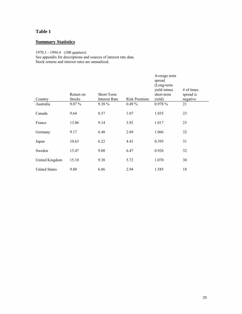
Table 1 shows the unconditional risk premiums of each country portfolio’s stock

returns in excess their short-term interest rate. All are positive. Table 1 also shows

summary statistics for the term spreads for each country. The average term spreads for

most of the countries lie in the range from 0.926 % for Sweden to 1.585 % for the US.

6

Japan’s average of 0.395% is unusual. Out of 100 quarters examined, the countries have

inverted yield curves ranging between 18 and 32 occurrences.

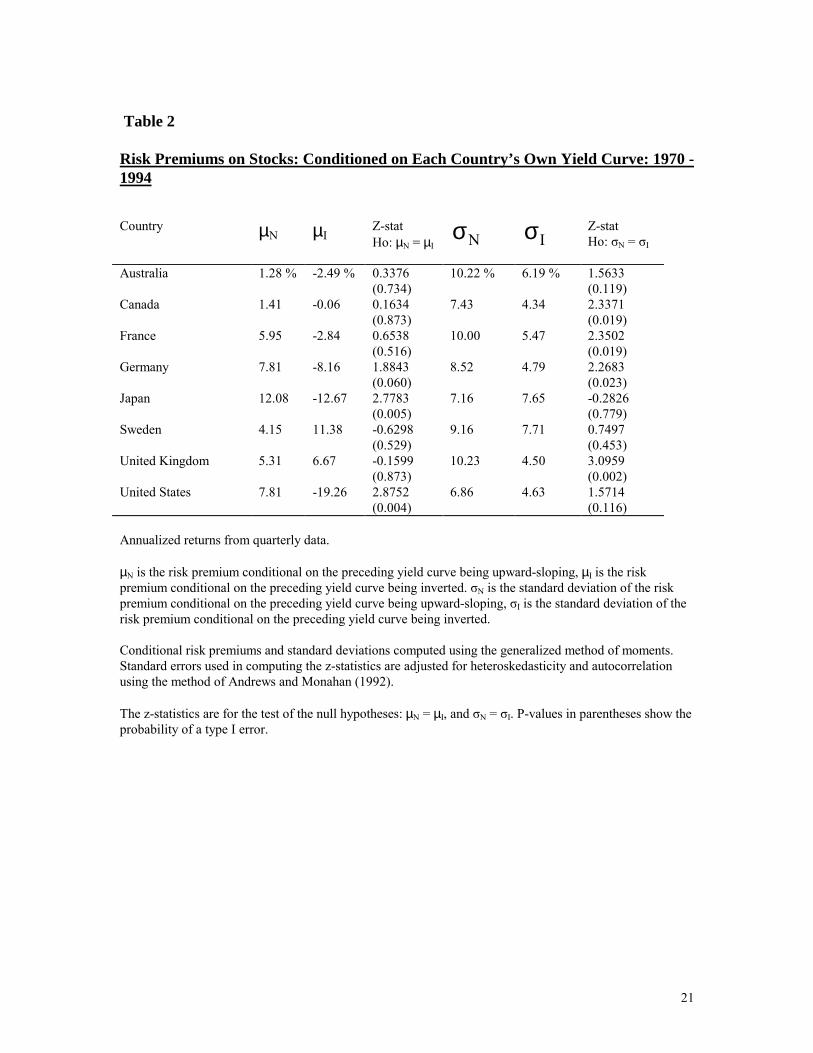
Table 2 shows the conditional risk premiums of each country’s stocks for periods

preceded by its own normal and inverted yield curves. The risk premiums are computed

using the generalized method of moments. A binary instrument for each country is

defined as St-1 = 1, if the term spread is positive, and St-1 = 0, if the term spread is

negative. This will give us the conditional risk premium for upward-sloping yield curves.

To compute the conditional risk premium for inverted yield curves: St-1 = 1 if the term

spread is negative and St-1 = 0 if the term spread is positive. The moment condition is:

( ) 0Sr 1tt =⊗µ− − . (1)

Where rt is the risk premium at time t and µ is the conditional mean risk premium being

computed. This method has the advantage of utilizing all of the data in order to estimate

the asymptotic distribution. Six out of eight of the country portfolios in the sample have

negative risk premiums when their yield curves are inverted. Z-statistics are computed for

the test of the null hypothesis µN = µI, where µN is the risk premium when the yield curve

is normal, and µI is the risk premium when the yield curve is inverted. These z-statistics

are computed using standard errors that are adjusted for heteroskedasticity and

autocorrelation using the method of Andrews and Monahan (1992). The z-statistics for

Japan, and the USA, are statistically significant at 99%. The statistic for Germany is

significant at 94% confidence. The stocks of Australia, Canada, and France also show

negative risk premiums when their yield curves are inverted, but are not statistically

significant. The stocks of Sweden and the UK show the risk premiums to be positive and

higher when their yield curves are inverted than when they are normal.

7

Why do the inverted yield curves signal statistically significant negative risk

premiums for only the three large economies? Estrella and Mishkin (1996) show how the

U.S. yield curve is a good predictor of business cycle fluctuations for the US.. The

probability of a recession increases as the term spread decreases. When the yield curve is

inverted (typically at the peak of a business cycle) the probability of a future recession is

at its highest. The yield curve inverts when the short-term interest rate rises above the

long-term rate, often caused by contractionary monetary policies that slow real growth

and hurt corporate profits in the near term. Since stock prices tend to rise and fall with

earnings and dividends, the yield curve also serves as a predictor of future stock returns.

To determine if there is a relation between the conditional risk premiums and their

volatility, the conditional standard deviations are computed and shown in Table 2. The

standard deviations and the z-statistics for their difference are computed using the same

methodology as was used for the means. All of the country portfolios except for Japan’s

show higher volatility during periods preceded by normal yield curves than during periods

preceded by inverted yield curves. The result for the U.S. is consistent with the finding of

Boudoukh, Richardson, and Whitelaw (1997), who find the volatility to be higher when

yield curve is upward-sloping, but they do not find the difference to be statistically

significant. This research finds the z-statistics for the differences between the two

conditional volatilities to be statistically significant for the stocks of Canada, France,

Germany, and the UK. The differences in the volatilities suggest that at least part of the

explanation for the higher risk premiums for the periods preceded by normal yield curves

is a compensation for the higher volatility. However, the results are not consistent.

Japanese stocks have lower risk premiums when their yield curve is inverted, but they

8

have higher volatility. Moreover, the lower volatilities that occur when the yield curves

are inverted do not justify a negative risk premium. Stocks are always a riskier investment

than Treasury Bills. A mean–variance framework cannot fully explain the phenomena,

but a consumption–based asset pricing model has the potential to do so.

Why do inverted yield curves signal statistically significant negative risk

premiums for only the largest economies? Exogenous international macroeconomic

shocks have a greater effect on the economies of smaller countries than on larger

countries. Crucini (1997) shows that larger economies have less volatile investment,

consumption, and trade balances, and higher correlations of domestic savings and

investment rates than smaller economies, due to the large economies’ stronger ability to

withstand international shocks. It stands to reason that the effects of these shocks will

also be felt more strongly in the small countries’ financial markets than in the large

countries. The shocks can obfuscate the relationship between the yield curve and returns

on stocks in the smaller countries. Sweden, which has the smallest economy in the

sample, has the highest conditional risk premiums when its own yield curve is inverted.

Since the small economies are susceptible to international shocks, do the yield curve

inversions in the larger economies also make their presence felt in the small countries?

The next step is to examine the relations between the larger countries’ yield curves and

the smaller countries’ risk premiums.

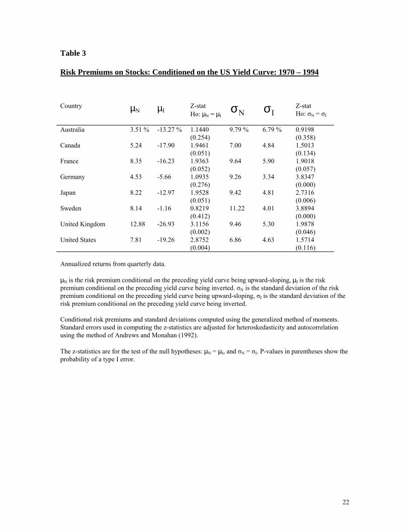
Table 3 shows the conditional risk premiums, for each country, for those periods

preceded by normal and inverted US yield curves. The differences from Table 2 are

striking. All of the countries except for Germany have lower conditional risk premiums

when the US term spread is used, instead of each country’s own term spread, and all are

9

negative. That the U.S. term spread could have such an impact is illustrated by the fact

that 56% of the world’s debt is dollar-denominated (The Wall Street Journal, March 22,

1996, p. C1.). If a foreign corporation has dollar-denominated debt, then the slope of the

U.S. yield curve will have an impact on its financing and investment decisions. The

results for the UK are particularly interesting. Risk premiums on UK stocks are negative

and statistically significant when conditioned on inverted U.S. yield curves, but are

positive when conditioned on inverted UK yield curves. The UK stock market has a

closer relationship with the U.S. yield curve than with the UK yield curve. Figure I shows

a graph of the time series of term spreads for the U.S. and UK.

Asprem (1989) regressed the stock returns for several European countries on the

U.S. term spread. He found a positive and statistically significant relationship for the

stock returns of Germany, the Netherlands, Switzerland, and the UK. His results are

consistent with the results of this research, since a positive relationship would imply a

low risk premium when the yield curve is inverted.

Table 3 also shows that the volatilities of the risk premiums are higher for all

eight country portfolios when the U.S. yield curve is upward-sloping, than when it is

inverted. The z-statistics for Germany, Japan, Sweden, and the UK are statistically

significant.

Table 4 shows the conditional risk premiums for those periods preceded by

inverted German yield curves for each country. The conditional risk premiums are

negative and significant for Australia, France, and Japan, and negative but insignificant

for the UK and the U.S. Figure II shows the graphs of the U.S. and German term spreads.

Both are negative at approximately the same times. One major exception is the second

10

quarter of 1980 that is positive for the US but negative for Germany. This instance,

caused by a rapid reversal of US monetary policy and the sudden imposition and

relaxation of credit controls, is an anomaly for the US. Another exception is the period

from 1991 to 1993, when German term spreads became negative while US term spreads

were positive. France, Sweden, and the UK also had inverted yield curves during most of

this period. Other researchers have noted the influence of German monetary policy on the

financial markets of the other European countries during this time period, but it is

interesting to see similar results for Australia and Japan. Gagnon and Unferth (1995) note

the similarity between the German and Japanese ex post real interest rates from 1977 to

1993. They also find that the German ex post real interest rate has the highest correlation

with their estimate of the world real interest rate. Comparing the results for the UK

between Tables 3 and 4 shows a tighter relation between the financial markets of the UK

and the U.S., than between the UK and Germany. The volatilities for all eight country

portfolios are greater when the German yield curve is upward–sloping than when it is

inverted. The z-statistics for the differences in the volatilities are statistically significant

for France, Germany, the UK, and the U.S.

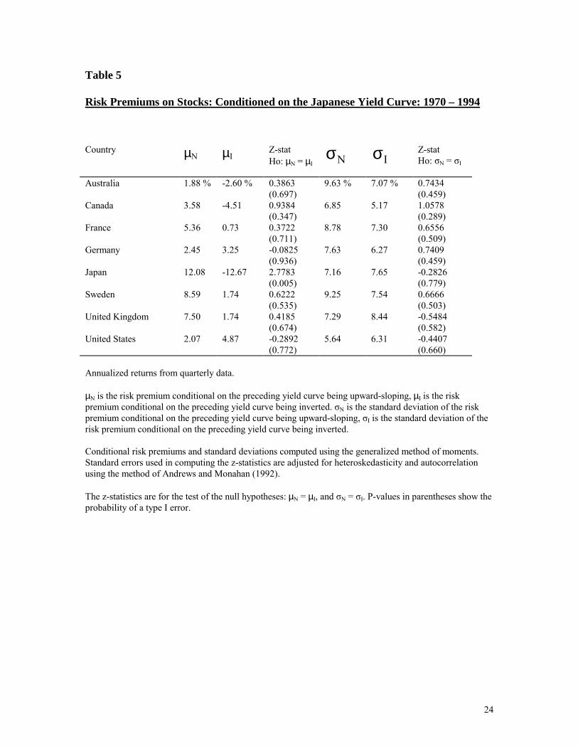
Table 5 shows the risk premiums conditioned on Japanese yield curves. All are

positive when preceded by an inverted yield curve except for those of Japan, Australia,

and Canada. The only statistically significant z-statistic is that of Japan. The Japanese

yield curve does not capture the world risk factor that is proxied by the US and German

yield curves, and suggests that the Japanese financial markets have a more isolated role in

the world economy than do the U.S. or Germany. Moreover, the volatilities for the

Japanese, British, and U.S. portfolios are higher when the Japanese yield curve is inverted

11

than when it is upward-sloping, and none of the eight z-statistics for the volatilities are

significant.

Ostdiek (1998) finds that the relation between the U.S. term spread and the risk

premium on the world portfolio varies by subperiod. She divides her 1970 – 1992 sample

in half and shows that the negative risk premiums are more prevalent in the 1970 – 1981

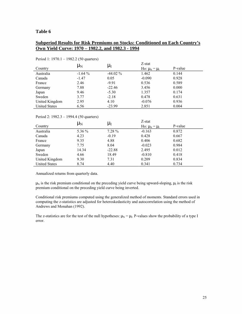
subperiod than in the 1981 – 1992 subperiod. For this research, the sample is also divided

into halves: 1970.1 – 1982.2, and 1982.3 – 1994.4. Each subperiod has 50 quarters. This

method of dividing the sample has the added attraction of beginning the second subperiod

just before the bull market of August, 1982 began.

Table 6 shows the subperiod results for the conditional risk premiums using each

country’s own yield curve. The first period shows results similar to the entire sample, but

only the German and U.S. z-statistics are statistically significant. The second subperiod

shows very different results. Only the Canadian and Japanese risk premiums are negative

when their yield curves invert, and only the Japanese z-statistic is significant. The results

for the U.S. are consistent with the subperiod results that Ostdiek finds for the world

portfolio. The only occasion during the second subperiod that the U.S. yield curve

inverted was during the last three quarters of 1989.

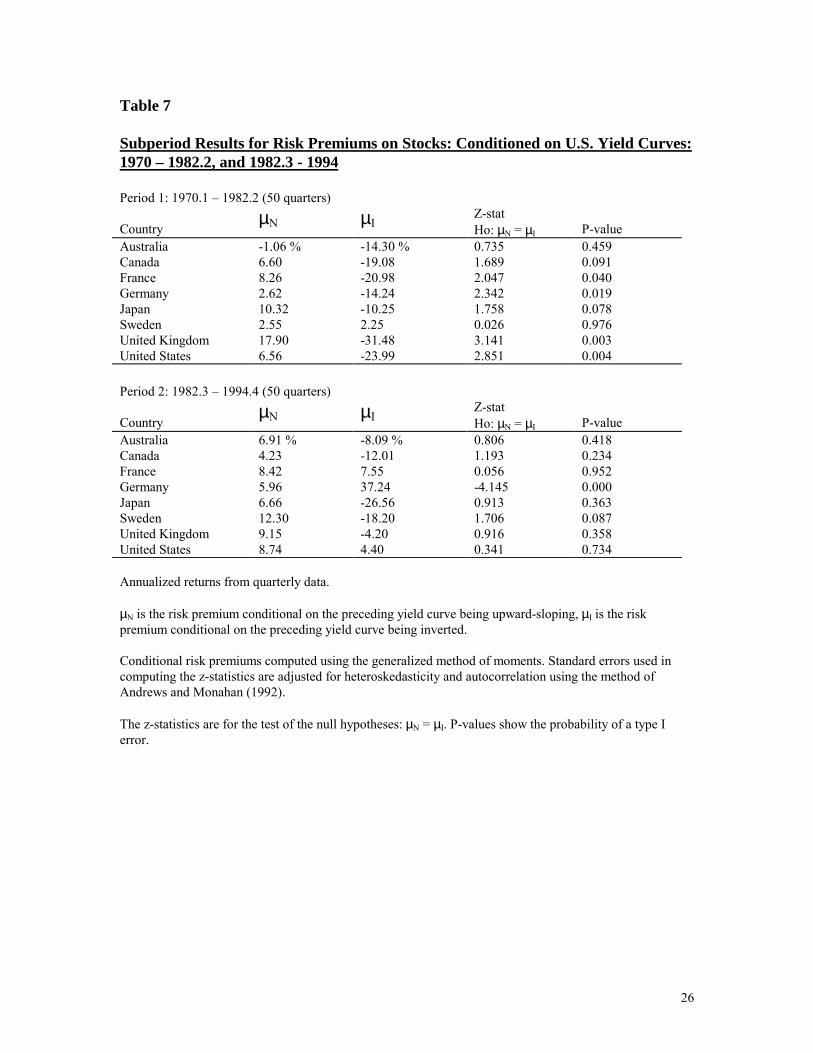
Table 7 shows the subperiod results using the U.S. yield curve as the conditioning

variable. During the first subperiod, all country portfolios have negative risk premiums

when the U.S. yield curve inverts, except for Sweden. The French, German, British, and

U.S. z-statistics are significant. During the second subperiod, five of the country

portfolios show the negative risk premiums, but none are both negative and statistically

12

significant. The German risk premium is positive and significant when the U.S. yield

curve inverts.

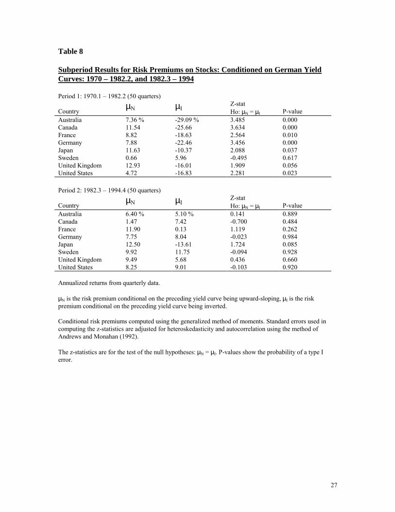
Table 8 shows the subperiod results using the German yield curve as the

conditioning variable. During the first subperiod, all country portfolios show negative risk

premiums when the German yield curve inverts, except for Sweden. The z-statistics for

Australia, Canada, France, Germany, Japan, and the U.S. are significant. During the

second subperiod, only the Japanese stocks show the negative conditional risk premiums

and they are not statistically significant.

Ostdiek (1998) suggests that the different subperiod results may be driven by the

power of the instruments in the different periods. She cites the fact that most of the U.S.

yield curve inversions occur during the first subperiod. This is also the case with the data

and subperiods used in this research. However, this is not the case for the German yield

curve. During the second subperiod, the German yield curve was inverted during 15 out

of 50 quarters, as compared with 17 out 50 quarters in the first subperiod.

Boudoukh, Richardson, and Whitelaw (1997) explore the risk premium – yield

curve relation further by testing for nonlinearity in the relation. One of the tests that they

run is a piecewise linear regression of the risk premium on the lagged term spread, using

a spread of zero for the breakpoint:

1t,tt,lf2t,lf11t ]r,0max[)r(rp ++ ε+∆β+∆β+α= . (2)

Boudoukh, Richardson, and Whitelaw find that the relation is nonlinear and concave for

the 1897 – 1990 period for the U.S. term spread and U.S. stocks. This research tests the

relation for nonlinearity using the same method for both each country’s own term spread

as well as the U.S. term spread.

13

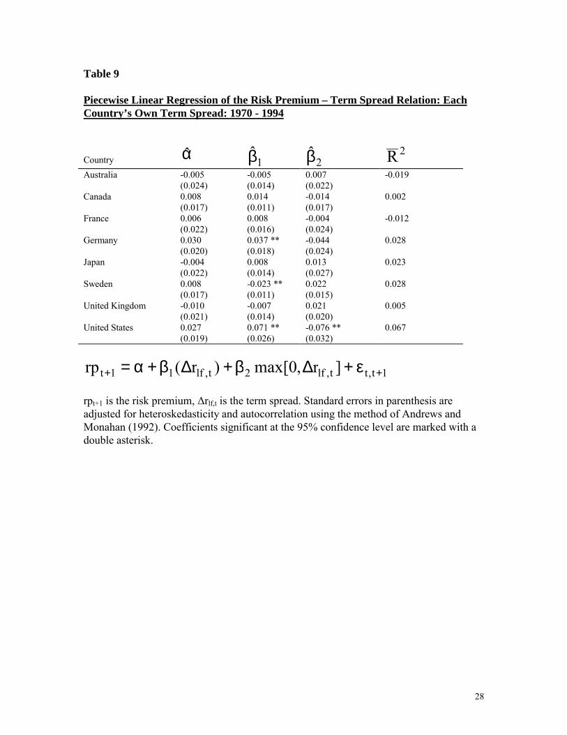
Table 9 shows the results for the test using each country’s own term spread as the

independent variable. Only the U.S. portfolio shows statistically significant slope

coefficients on both sides of the breakpoint. The coefficients are positive for a negative

term spread and negative for a positive term spread, implying a concave relation, just as

Boudoukh, Richardson, and Whitelaw find for their longer data set. The results for the

German portfolio are similar, but the coefficient for the positive term spread is not

statistically significant. The results for Sweden imply a convex relation, but again the

second slope coefficient is not significant.

Table 10 shows the results for all eight country portfolios, using the U.S. term

spread as the independent variable. All eight portfolios have a positive point estimate for

the first slope coefficient and a negative estimate for the second, implying a concave

relationship. The Canadian, UK, and U.S. portfolios have statistically significant results

for both slope coefficients. Overall the results shown in Table 9 and 10 are consistent

with the findings of Boudoukh, Richardson, and Whitelaw (1997), but only show that the

U.S. term spread has this effect.

IV. The Relations Between Risk Premiums and Consumption

The yield curves of Germany, Japan, and the U.S. can be used to forecast negative

risk premiums for their respective stocks, and the German and U.S. yield curves can be

used to forecast negative risk premiums for the other countries’ stocks. Boudoukh,

Richardson, and Smith (1993) show that this phenomenon also holds for annual returns

for US stocks. They also show that this relationship is an ancient one: their data set runs

14

from 1802 to 1990. This section investigates whether this phenomenon be explained by

asset pricing theory.

In one-period capital asset pricing models such as the conditional version of the

CAPM, if investors are risk averse then the expected return on the market of risky assets

must be greater than the return on risk free assets:

Et [Rm,t+1] ≥ Rft

(3) where Rm,t+1 is the return on the market portfolio from time t to t+1 and Rft is

the return on the risk free asset from time t to t+1. Et is the expectation operator as of time

t, conditional on the information investors use to form their expectations. A potential

problem with testing this prediction of the CAPM, as suggested by Roll (1977) is that the

true market portfolio is unobservable. We are restricted to testing returns of a proxy of the

market portfolio: Rpt+1. However, this is not a problem if the conditional covariance

between the proxy and the true market portfolio is positive. If the conditional CAPM

holds, then it must be true that:

E R RR R

RE R Rt pt ft

t pt mt

t mtt mt ft[( )]

cov [ , ]var [ ]

[( )]++ +

++− = −1

1 1

11 (4)

Therefore, if the market risk premium is positive, and the conditional covariance is

positive, then the risk premium on the proxy portfolio must also be positive. Thus, each

country’s stock portfolio should have a positive ex ante risk premium at all times,

provided that it is positively correlated with the world market portfolio of all assets. The

correlations between the returns on the stock portfolios for each pair of countries in the

sample were computed (not shown). All of the correlations are positive and statistically

significant.

15

The results of Boudoukh, Richardson, and Smith (1993), Ostdiek (1998), and this

research do not support the inequality constraint of equation (3). The CAPM is a one

period model that assumes that an investor’s consumption is equal to the gross return

from her investments. A dynamic, consumption-based asset pricing model, such as

Breeden's (1979) CCAPM, can result in a negative risk premium for any asset, including

the market portfolio. The first-order conditions for an individual’s optimal consumption

and portfolio plan imply that:

E R R U' CU' Ct it ft

t

t( ) ( )

( )++− � �

�

�� =1

1 0 (5)

where U'(.) is marginal utility and Ct is consumption at time t. The expression

U CU C

t

t

' ( )' ( )

+1 is the intertemporal marginal rate of substitution (IMRS) which will be

abbreviated as Mt+1. Rit+1 is the return on any risky asset, which could be the market

portfolio.

Taking a first-order Taylor series expansion of the numerator of the IMRS around

Ct gives us:

)C('U)C(''U)CC()C('U

)C('U)C('U

t

tt1tt

t

1t −+≈ ++ . (6)

Rearranging the RHS of (3) we get:

��

� −��

��

� −−=

−+ ++

t

t1t

t

tt

t

tt1ttC

CC)C('U

)C(''UC1

)C('U)C(''U)CC()C('U

. (7)

Let �

��

� −=

)C('U)C(''UC

bt

tt denote the aggregate relative risk aversion, which is

nonstochastic because it depends only on Ct, which is known at time t. Let

16

��

� −= +

+t

t1t*1t C

CCc denote the growth rate of consumption. Combine equation (5) with

equations (6) and (7), and ignore the approximation to get:

0)]bc1)(RR[(E *1tft1t,it =−− ++ . (8)

Applying the definition of covariance, rearranging, and taking the limit to continuous

time we get:

E R R bCov R R ct i t ft t i t ft t[ ] ( , ), ,*

+ + +− = −1 1 1 (9)

Equation (9) suggests two possible explanations for negative ex ante risk premiums: the

covariance between the risk premium and the growth rate of consumption might be

negative in those states of the world, or the relative risk aversion might be negative, but

not both. If both are positive or both are negative, then the risk premium will be positive.

Over the long run the covariance in (9) should be positive, but Cornell (1981) has

shown that the conditional relationship need not be constant. It is theoretically possible

for the relationship to be positive in some states of the world and negative in others.

Boudoukh, Richardson, and Whitelaw (1997) develop a stylized model that

assumes that consumption and dividend growth follow a discrete Markov process. They

show that, given the right assumptions about the parameters of the process, the equity

returns will act as a hedge to consumption shocks and that therefore investors will be

willing to accept negative expected risk premiums on equities. However, they are merely

showing that it can happen. This research concerns the question of whether or not it

actually is happening. Boudoukh, Richardson, and Whitelaw do not perform any

empirical tests on the consumption data at all.

17

The next step of this research is to determine if the sign of the risk premiums can

be explained by the sign of their covariance with the growth rate of consumption. Per

equation (9), the CCAPM predicts that the sign of the risk premium should be the same as

the sign of the covariance between consumption growth and the risk premium, assuming

risk aversion. Table 11 shows the conditional covariances between consumption growth

and the risk premiums on stocks for each country, for those periods preceded by their own

inverted yield curves. The conditional covariances are computed using the generalized

method of moments. GMM relies on the assumption that the variables being tested are

stationary. The time series of the risk premiums of the assets as well as the consumption

growth rates were tested for stationarity (not shown). All of the time series strongly

rejected the null hypothesis of unit root nonstationarity. In order to compute the

covariances, it is necessary to estimate three moments: the mean risk premium, the mean

consumption growth rate, and the mean of the product of the two variables:

.0S

*rccr

*cc

rr

1t*tt

*t

t

=⊗

�

��

�

�

−

−

−

− (10)

Where St-1 = 0 if the preceding yield curve is normal, 1 if inverted. The conditional

covariance is then computed as:

( ) *cr'tt*rc

'ttc,rCov

2*ttt ⋅�

��

�−��

��

�= . (11)

Where t is the total number of periods in the sample, and t’ is the number of periods

preceded by inverted yield curves. Robust standard errors are computed using the method

of Andrews and Monahan (1992). All of the covariances in Table 11 are statistically

18

indifferent from zero. Many researchers have found that the relationship between stock

returns and aggregate consumption growth is very weak for the U.S. It is not surprising

that this should also prove to be the case for the foreign countries.

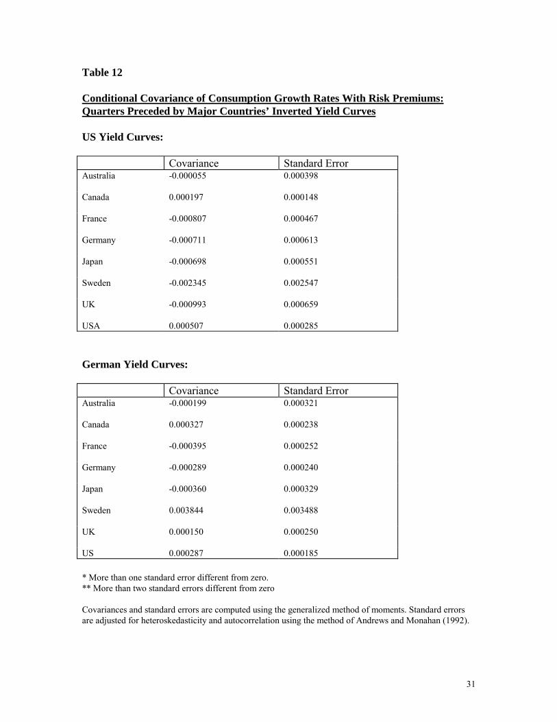
Table 12 shows the covariances using the US or German yield curves as the

conditioning variable. The results are similar to Table 11. The CCAPM cannot explain

why investors are willing to accept the negative risk premiums. Even if the cause of the

failure of the test were lack of power, the point estimates of the covariances do not

support equation (9) in most cases. For example, U.S. stocks show negative risk

premiums when the U.S. yield curve is inverted, but the conditional covariance is

positive. For equation (9) to hold with a positive covariance, the coefficient of relative

risk aversion would have to be negative. There are certainly some investors who are risk-

loving, but it is unlikely that most are.

V. Conclusions

Negative, statistically significant risk premiums occur for U.S., German and

Japanese stocks during periods preceded by their own inverted yield curves. This

phenomenon is not found for the smaller economies in the sample. In particular, Sweden,

and the UK have positive risk premiums in such periods. The effects of the German and

U.S. yield curves on the smaller country’s stocks show evidence of international

transmission of shocks to financial asset markets. Many of the smaller economies have

negative risk premiums in periods preceded by inverted German or U.S. yield curves. An

examination of the graphs of the U.S. and German term spreads shows that they become

19

negative during approximately the same time periods. The Japanese yield curve does not

show this relation with the smaller countries’ stock returns.

For most of the country portfolios, the volatility of the risk premiums tends to be

lower when either each country’s own yield curve, or the U.S. or German yield curves are

inverted. This is not the case for the Japanese yield curve.

Tests for nonlinearity in the risk premium-term spread relation show that the U.S.

term spread shows a concave relation with U.S., Canadian, and British equities.

The CCAPM is not able to explain the phenomenon of the negative risk

premiums. The conditional covariance between the risk premium and consumption

growth is statistically insignificant from zero.

Future research should investigate what international risk factor is being

transmitted across financial markets. Are the negative risk premiums a result of US

and/or German monetary policy, or are real shocks involved? It would also be interesting

to solve the puzzle of why investors are willing to accept the ex ante negative risk

premiums.

20

Table 1

Summary Statistics

1970.1 - 1994.4 (100 quarters)See appendix for descriptions and sources of interest rate data.Stock returns and interest rates are annualized.

CountryReturn onStocks

Short-TermInterest Rate Risk Premium

Average termspread(Long-termyield minusshort-termyield)

# of timesspread isnegative

Australia 9.87 % 9.38 % 0.49 % 0.978 % 21

Canada 9.64 8.57 1.07 1.035 23

France 13.06 9.14 3.92 1.017 23

Germany 9.17 6.48 2.69 1.066 32

Japan 10.63 6.22 4.41 0.395 31

Sweden 15.47 9.00 6.47 0.926 32

United Kingdom 15.10 9.38 5.72 1.070 30

United States 9.80 6.86 2.94 1.585 18

21

Table 2

Risk Premiums on Stocks: Conditioned on Each Country’s Own Yield Curve: 1970 -1994

Country µN µIZ-statHo: µN = µI Nσ Iσ Z-stat

Ho: σN = σI

Australia 1.28 % -2.49 % 0.3376(0.734)

10.22 % 6.19 % 1.5633(0.119)

Canada 1.41 -0.06 0.1634(0.873)

7.43 4.34 2.3371(0.019)

France 5.95 -2.84 0.6538(0.516)

10.00 5.47 2.3502(0.019)

Germany 7.81 -8.16 1.8843(0.060)

8.52 4.79 2.2683(0.023)

Japan 12.08 -12.67 2.7783(0.005)

7.16 7.65 -0.2826(0.779)

Sweden 4.15 11.38 -0.6298(0.529)

9.16 7.71 0.7497(0.453)

United Kingdom 5.31 6.67 -0.1599(0.873)

10.23 4.50 3.0959(0.002)

United States 7.81 -19.26 2.8752(0.004)

6.86 4.63 1.5714(0.116)

Annualized returns from quarterly data.

µN is the risk premium conditional on the preceding yield curve being upward-sloping, µI is the riskpremium conditional on the preceding yield curve being inverted. σN is the standard deviation of the riskpremium conditional on the preceding yield curve being upward-sloping, σI is the standard deviation of therisk premium conditional on the preceding yield curve being inverted.

Conditional risk premiums and standard deviations computed using the generalized method of moments.Standard errors used in computing the z-statistics are adjusted for heteroskedasticity and autocorrelationusing the method of Andrews and Monahan (1992).

The z-statistics are for the test of the null hypotheses: µN = µI, and σN = σI. P-values in parentheses show theprobability of a type I error.

22

Table 3

Risk Premiums on Stocks: Conditioned on the US Yield Curve: 1970 – 1994


Ho: σN = σI

Australia 3.51 % -13.27 % 1.1440(0.254)

9.79 % 6.79 % 0.9198(0.358)

Canada 5.24 -17.90 1.9461(0.051)

7.00 4.84 1.5013(0.134)

France 8.35 -16.23 1.9363(0.052)

9.64 5.90 1.9018(0.057)

Germany 4.53 -5.66 1.0935(0.276)

9.26 3.34 3.8347(0.000)

Japan 8.22 -12.97 1.9528(0.051)

9.42 4.81 2.7316(0.006)

Sweden 8.14 -1.16 0.8219(0.412)

11.22 4.01 3.8894(0.000)

United Kingdom 12.88 -26.93 3.1156(0.002)

9.46 5.30 1.9878(0.046)

United States 7.81 -19.26 2.8752(0.004)

6.86 4.63 1.5714(0.116)





23

Table 4

Risk Premiums on Stocks: Conditioned on the German Yield Curve: 1970 – 1994


Ho: σN = σI

Australia 6.87 % -13.06 % 2.3629(0.018)

10.18 % 6.06 % 1.8256(0.067)

Canada 2.22 4.54 -1.6900(0.091)

6.09 5.93 0.1254(0.904)

France 10.40 -9.83 2.5166(0.012)

10.03 5.19 2.6664(0.008)

Germany 7.81 -8.16 1.8843(0.060)

8.52 4.79 2.2683(0.023)

Japan 12.07 -11.88 2.7010(0.007)

8.78 5.74 1.8397(0.066)

Sweden 5.42 8.67 -0.2964(0.764)

9.33 7.50 0.7959(0.424)

United Kingdom 11.16 -5.84 1.7969(0.072)

10.02 4.68 2.5605(0.010)

United States 6.54 -4.71 1.5146(0.131)

7.28 4.18 2.4372(0.015)





24

Table 5

Risk Premiums on Stocks: Conditioned on the Japanese Yield Curve: 1970 – 1994


Ho: σN = σI

Australia 1.88 % -2.60 % 0.3863(0.697)

9.63 % 7.07 % 0.7434(0.459)

Canada 3.58 -4.51 0.9384(0.347)

6.85 5.17 1.0578(0.289)

France 5.36 0.73 0.3722(0.711)

8.78 7.30 0.6556(0.509)

Germany 2.45 3.25 -0.0825(0.936)

7.63 6.27 0.7409(0.459)

Japan 12.08 -12.67 2.7783(0.005)

7.16 7.65 -0.2826(0.779)

Sweden 8.59 1.74 0.6222(0.535)

9.25 7.54 0.6666(0.503)

United Kingdom 7.50 1.74 0.4185(0.674)

7.29 8.44 -0.5484(0.582)

United States 2.07 4.87 -0.2892(0.772)

5.64 6.31 -0.4407(0.660)





25

Table 6

Subperiod Results for Risk Premiums on Stocks: Conditioned on Each Country’sOwn Yield Curve: 1970 – 1982.2, and 1982.3 - 1994

Period 1: 1970.1 – 1982.2 (50 quarters)

CountryµN µI

Z-statHo: µN = µI P-value

Australia -1.64 % -44.02 % 1.462 0.144Canada -1.47 0.05 -0.090 0.928France 2.46 -9.91 0.536 0.589Germany 7.88 -22.46 3.456 0.000Japan 9.46 -5.30 1.357 0.174Sweden 3.77 -2.18 0.478 0.631United Kingdom 2.95 4.10 -0.076 0.936United States 6.56 -23.99 2.851 0.004

Period 2: 1982.3 – 1994.4 (50 quarters)

CountryµN µI


Australia 5.36 % 7.28 % -0.163 0.872Canada 4.23 -0.19 0.428 0.667France 9.35 4.88 0.406 0.682Germany 7.75 8.04 -0.023 0.984Japan 14.34 -22.88 2.495 0.012Sweden 4.66 18.49 -0.810 0.418United Kingdom 9.30 7.31 0.209 0.834United States 8.74 4.40 0.341 0.734


µN is the risk premium conditional on the preceding yield curve being upward-sloping, µI is the riskpremium conditional on the preceding yield curve being inverted.

Conditional risk premiums computed using the generalized method of moments. Standard errors used incomputing the z-statistics are adjusted for heteroskedasticity and autocorrelation using the method ofAndrews and Monahan (1992).

The z-statistics are for the test of the null hypotheses: µN = µI. P-values show the probability of a type Ierror.

26

Table 7

Subperiod Results for Risk Premiums on Stocks: Conditioned on U.S. Yield Curves:1970 – 1982.2, and 1982.3 - 1994

Period 1: 1970.1 – 1982.2 (50 quarters)

CountryµN µI


Australia -1.06 % -14.30 % 0.735 0.459Canada 6.60 -19.08 1.689 0.091France 8.26 -20.98 2.047 0.040Germany 2.62 -14.24 2.342 0.019Japan 10.32 -10.25 1.758 0.078Sweden 2.55 2.25 0.026 0.976United Kingdom 17.90 -31.48 3.141 0.003United States 6.56 -23.99 2.851 0.004

Period 2: 1982.3 – 1994.4 (50 quarters)

CountryµN µI


Australia 6.91 % -8.09 % 0.806 0.418Canada 4.23 -12.01 1.193 0.234France 8.42 7.55 0.056 0.952Germany 5.96 37.24 -4.145 0.000Japan 6.66 -26.56 0.913 0.363Sweden 12.30 -18.20 1.706 0.087United Kingdom 9.15 -4.20 0.916 0.358United States 8.74 4.40 0.341 0.734





27

Table 8

Subperiod Results for Risk Premiums on Stocks: Conditioned on German YieldCurves: 1970 – 1982.2, and 1982.3 – 1994

Period 1: 1970.1 – 1982.2 (50 quarters)

CountryµN µI


Australia 7.36 % -29.09 % 3.485 0.000Canada 11.54 -25.66 3.634 0.000France 8.82 -18.63 2.564 0.010Germany 7.88 -22.46 3.456 0.000Japan 11.63 -10.37 2.088 0.037Sweden 0.66 5.96 -0.495 0.617United Kingdom 12.93 -16.01 1.909 0.056United States 4.72 -16.83 2.281 0.023

Period 2: 1982.3 – 1994.4 (50 quarters)

CountryµN µI


Australia 6.40 % 5.10 % 0.141 0.889Canada 1.47 7.42 -0.700 0.484France 11.90 0.13 1.119 0.262Germany 7.75 8.04 -0.023 0.984Japan 12.50 -13.61 1.724 0.085Sweden 9.92 11.75 -0.094 0.928United Kingdom 9.49 5.68 0.436 0.660United States 8.25 9.01 -0.103 0.920





28

Table 9

Piecewise Linear Regression of the Risk Premium – Term Spread Relation: EachCountry’s Own Term Spread: 1970 - 1994

Country α̂ 1β̂ 2β̂ 2RAustralia -0.005

(0.024)-0.005(0.014)

0.007(0.022)

-0.019

Canada 0.008(0.017)

0.014(0.011)

-0.014(0.017)

0.002

France 0.006(0.022)

0.008(0.016)

-0.004(0.024)

-0.012

Germany 0.030(0.020)

0.037 **(0.018)

-0.044(0.024)

0.028

Japan -0.004(0.022)

0.008(0.014)

0.013(0.027)

0.023

Sweden 0.008(0.017)

-0.023 **(0.011)

0.022(0.015)

0.028

United Kingdom -0.010(0.021)

-0.007(0.014)

0.021(0.020)

0.005

United States 0.027(0.019)

0.071 **(0.026)

-0.076 **(0.032)

0.067

1t,tt,lf2t,lf11t ]r,0max[)r(rp ++ ε+∆β+∆β+α=

rpt+1 is the risk premium, ∆rlf,t is the term spread. Standard errors in parenthesis areadjusted for heteroskedasticity and autocorrelation using the method of Andrews andMonahan (1992). Coefficients significant at the 95% confidence level are marked with adouble asterisk.

29

Table 10

Piecewise Linear Regression of the Risk Premium – Term Spread Relation: U.S.Term Spreads: 1970 - 1994

Country α̂ 1β̂ 2β̂ 2RAustralia 0.009

(0.028)0.037(0.039)

-0.038(0.047)

-0.007

Canada 0.029(0.020)

0.066 **(0.027)

-0.074 **(0.033)

0.039

France 0.018(0.027)

0.045(0.037)

-0.045(0.044)

0.002

Germany 0.002(0.023)

0.021(0.032)

-0.017(0.039)

-0.005

Japan 0.008(0.025)

0.037(0.034)

-0.032(00.042)

0.010

Sweden 0.015(0.029)

0.007(0.039)

-0.006(0.047)

-0.020

United Kingdom 0.056 **(0.025)

0.111 **(0.034)

-0.124 **(0.042)

0.084

United States 0.027(0.019)

0.071 **(0.026)

-0.076 **(0.032)

0.067

1t,tt,lf2t,lf11t ]r,0max[)r(rp ++ ε+∆β+∆β+α=

rpt+1 is the risk premium, ∆rlf,t is the term spread. Standard errors in parenthesis areadjusted for heteroskedasticity and autocorrelation using the method of Andrews andMonahan (1992). Coefficients significant at the 95% confidence level are marked with adouble asterisk.

30

Table 11

Conditional Covariance of Consumption Growth Rates With Risk Premiums:Quarters Preceded by Each Countries’ Inverted Yield Curve

Covariance Standard ErrorAustralia -0.000448 0.000301

Canada 0.000075 0.000263

France -0.000366 0.000352

Germany -0.000289 0.000240

Japan -0.000495 0.000349

Sweden 0.002621 0.003489

UK 0.000095 0.000416

USA 0.000507 0.000285

Covariances and standard errors are computed using the generalized method of moments. Standard errorsare adjusted for heteroskedasticity and autocorrelation using the method of Andrews and Monahan (1992).

31

Table 12

Conditional Covariance of Consumption Growth Rates With Risk Premiums:Quarters Preceded by Major Countries’ Inverted Yield Curves

US Yield Curves:


Canada 0.000197 0.000148

France -0.000807 0.000467

Germany -0.000711 0.000613

Japan -0.000698 0.000551

Sweden -0.002345 0.002547

UK -0.000993 0.000659

USA 0.000507 0.000285

German Yield Curves:


Canada 0.000327 0.000238

France -0.000395 0.000252

Germany -0.000289 0.000240

Japan -0.000360 0.000329

Sweden 0.003844 0.003488

UK 0.000150 0.000250

US 0.000287 0.000185

* More than one standard error different from zero.** More than two standard errors different from zero

Covariances and standard errors are computed using the generalized method of moments. Standard errorsare adjusted for heteroskedasticity and autocorrelation using the method of Andrews and Monahan (1992).

32

Appendix

Descriptions and Sources of Interest Rate Data

CountryLong-Term Rate:Description Source

Short-Term Rate:Description Source

Australia 10 year Treasury Bonds Reserve Bankof Australia,MonthlyStatisticalBulletin

13 week TreasuryNote

IFS

Canada Government Bonds > 10years

IFS 3 month TreasuryBills

IFS

France 10 Year Government Bonds GlobalFinancial Data,Inc.

Call Money Rate IFS

Germany 1970 – 1975: 5 year FederalBonds

1976 – 1994: 10 yearFederal Bonds

DRI/McGraw-Hill

DeutscheBundesbank,Monthly Report

3 month InterbankRate

IFS

Japan 1970 – 1980: 7 yearGovernment Bonds

1980 – 1994: 10 yearGovernment Bonds

DRI/McGraw-Hill

Bank of Japan,EconomicStatisticsMonthly

Call Money MarketRate

IFS

Sweden 10 Year Government BondYield

SverigesRiksbank,QuarterlyReview

3 month TreasuryDiscount Notes

IFS

United Kingdom 10 Year Government BondYield

CentralStatisticalOffice, AnnualAbstract ofStatistics, andthe FinancialTimes

91 Day TreasuryBill Rate

IFS

United States 10 Year Government BondYield

FederalReserve, Boardof Governors

Quarterly TreasuryBill Rate

IFS

33

References

Andrews, D.W.K., and J.C. Monahan, 1992, An improved heteroskedasticity andautocorrelation consistent covariance matrix estimator, Econometrica 60, 953-966.

Asprem, Mads, 1989, Stock prices, asset portfolios and macroeconomic variables in tenEuropean countries, Journal of Banking and Finance 13, 589-612.

Breeden, Douglas, 1979, An intertemporal asset pricing model with stochasticconsumption and investment opportunities, Journal of Financial Economics 7, 265-296.

Breeden, Douglas, Michael Gibbons, and Robert Litzenberger, 1989, Empirical tests ofthe consumption-oriented CAPM, Journal of Finance 44, 231-262.

Boudoukh, Jacob, Matthew Richardson, and Tom Smith, 1993, Is the ex ante riskpremium positive? A new approach to testing conditional asset pricing models, Journal ofFinancial Economics 34, 387-408.

Boudoukh, Jacob, Matthew Richardson, and Robert Whitelaw, 1997, Nonlinearities in therelation between the equity risk premium and the term structure, Management Science 43,371 – 385.

Cornell, B., 1981, The consumption based asset pricing model: A note on potential testsand applications, Journal of Financial Economics 9, 103 - 108.

Crucini, Mario, 1997, Country size and economic fluctuations, Review of InternationalEconomics 5, 204 – 220.

Estrella, Arturo and Frederic Mishkin, 1996, The yield curve as a predictor of USrecessions, Current Issues in Economics and Finance 2, Federal Reserve Bank of NewYork.

Fama, Eugene and Kenneth French, 1989, Business conditions and expected returns onstocks and bonds, Journal of Financial Economics 25, 23-49.

Gagnon, Joseph E. and Mark D. Unferth, 1995, Is there a world real interest rate?, Journalof International Money and Finance 14, 845-855.

McCown, James Ross, 1999, The effects of inverted yield curves on asset returns,Financial Review 34, 109 – 126.

Ostdiek, Barbara, 1998, The world ex ante risk premium: an empirical investigation,Journal of International Money and Finance 17, 967 - 999.

34

Roll, Richard, 1977, A critique of the asset pricing theories tests, Journal of FinancialEconomics 4, 129-176.

yield curves and international equity returns i. introduction many researchers have investigated the...

Documents