1

Computer Tools for Data Analysis & Presentation Graphs All public machines on campus are now equipped with Word 2010 and Excel 2010. Although fancier graphical and statistical analysis programs exist, Excel should be sufficient for the purposes of FSBio 201.

Some Elements of a Complete, Informative Graph 1. Title or Figure Legend

Figures appearing in publication typically do not have titles, but have a descriptive ‘figure legend’ text below. What are the variables? What do the error bars represent? What are the sample sizes? You may want to include the statistical significance (p-value).

Figures used in presentations often have titles in lieu of a complete figure legend. 2. Axes

What is the variable being depicted? What are its units? Is the axis re-scaled? Is the axis log-transformed? Is the scale range appropriate? Are the tick marks appropriately spaced?

3. Numbers

Are an appropriate number of decimal places displayed? 4. Background and Gridlines

You should consider using a simple white background and no gridlines, although other backgrounds and presence of gridlines may be appropriate for some graphs.

5. Trendline Equation

You may need to change the number of displayed decimals. Be sure to also display the R2 value. 6. Symbols and Fonts

Symbols and fonts can be altered as to size, form, and color to increase readability and improve appearance. Use appropriate symbols to enhance your presentation – for example, red for data from a warm environment compared to blue for a cold environment, or white for exposure to light and black for a dark environment.

7. Legend

When only one series of data is displayed, the ‘symbol legend’ is unnecessary and should be deleted. When more than one series of data is displayed, a ‘symbol legend’ may be helpful to label the series appropriately.

You are to turn in the following three graphs at the beginning of class on Wednesday, January 21.

1) Reproduce the bar chart in Figure 2.10 of the bar chart tutorial of ATR for residents and intruders for the three size classes using the data given in the bar chart tutorial.

2) Reproduce the X-Y scatterplot in Figure 3.5 plot using the “Food consumed” vs “Mass” data

of the X-Y tutorial. Include a trendline with the regression equation and R2 value. 3) Reproduce the X-Y scatterplot with two series in Figure 3.6 using the data in the table.

Be sure to properly format and label the axes for each graph.

2

Figure 1.2

1

1

2

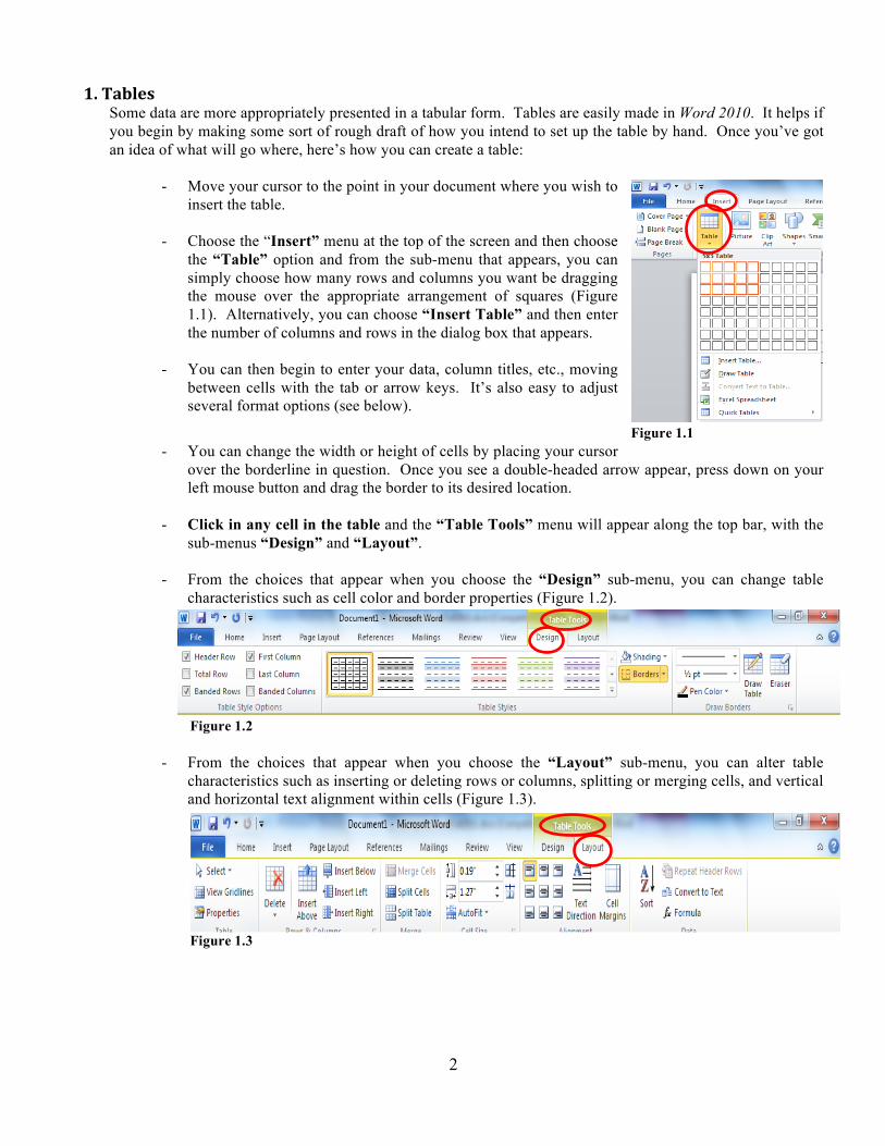
1.  Tables  Some data are more appropriately presented in a tabular form. Tables are easily made in Word 2010. It helps if you begin by making some sort of rough draft of how you intend to set up the table by hand. Once you’ve got an idea of what will go where, here’s how you can create a table:

- Move your cursor to the point in your document where you wish to insert the table.

- Choose the “Insert” menu at the top of the screen and then choose

the “Table” option and from the sub-menu that appears, you can simply choose how many rows and columns you want be dragging the mouse over the appropriate arrangement of squares (Figure 1.1). Alternatively, you can choose “Insert Table” and then enter the number of columns and rows in the dialog box that appears.

- You can then begin to enter your data, column titles, etc., moving between cells with the tab or arrow keys. It’s also easy to adjust several format options (see below).

- You can change the width or height of cells by placing your cursor

over the borderline in question. Once you see a double-headed arrow appear, press down on your left mouse button and drag the border to its desired location.

- Click in any cell in the table and the “Table Tools” menu will appear along the top bar, with the

sub-menus “Design” and “Layout”.

- From the choices that appear when you choose the “Design” sub-menu, you can change table characteristics such as cell color and border properties (Figure 1.2).

- From the choices that appear when you choose the “Layout” sub-menu, you can alter table characteristics such as inserting or deleting rows or columns, splitting or merging cells, and vertical and horizontal text alignment within cells (Figure 1.3).

Figure 1.1

Figure 1.3

22

3

2. Creating Bar Graphs with Excel 2010

Biologists frequently use bar graphs to summarize and present the results of their research. This tutorial will show you how to generate these kinds of graphs (with error bars) using a biologically relevant student-generated data set. As part of her senior thesis research on territoriality in the Mountain Dusky Salamander (Desmognathus ochrophaeus), Samantha Witchell (Class of 1999) investigated the role of prior occupancy on the outcome of territorial interactions and aggressive behavior. Samantha staged encounters between a male that had been allowed to establish a territory in a laboratory arena (“resident”) and a comparably sized male without any prior residency (“intruder”). In order to control for the effects of body size, males were categorized into three size classes; small one-year-old males (30-33 mm snout-vent length), medium-sized two-year-old males (36-39 mm), and large adult males (42-45 mm). The resident and intruder used in a particular trial were matched by size, and Samantha staged a total of eight encounters for each of the three size classes. In each trial, Samantha allowed the two salamanders to interact with each other for 20 minutes, during which time she collected data on several different behaviors. One of the behaviors she recorded was the “all trunk raised” (ATR) posture, an aggressive posture used by males in territorial encounters. Here are data she collected on the number of ATR postures performed by residents and intruders.

30-33 mm 36-39 mm 42-45 mm Trial Resident Intruder Resident Intruder Resident Intruder

1 1 0 3 0 4 1 2 2 0 2 0 2 0 3 0 0 2 1 2 0 4 1 0 1 0 1 0 5 0 1 2 1 3 1 6 0 0 1 0 1 2 7 0 0 0 0 2 0 8 0 0 3 0 2 0

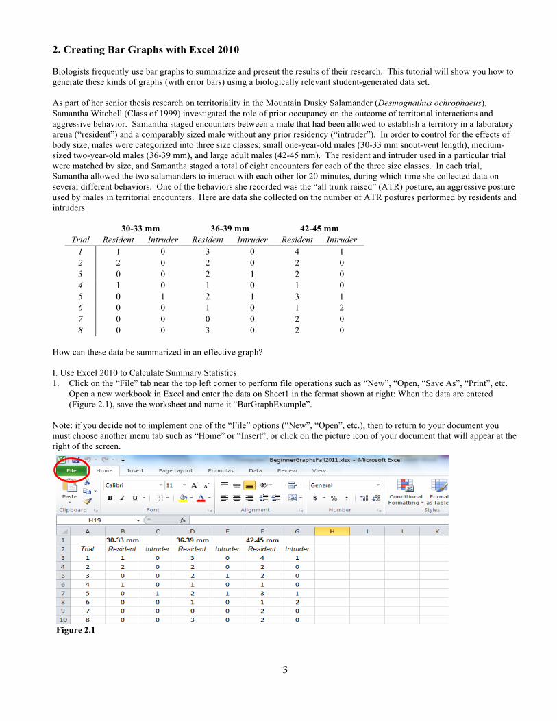
How can these data be summarized in an effective graph? I. Use Excel 2010 to Calculate Summary Statistics 1. Click on the “File” tab near the top left corner to perform file operations such as “New”, “Open, “Save As”, “Print”, etc.

Open a new workbook in Excel and enter the data on Sheet1 in the format shown at right: When the data are entered (Figure 2.1), save the worksheet and name it “BarGraphExample”.

Note: if you decide not to implement one of the “File” options (“New”, “Open”, etc.), then to return to your document you must choose another menu tab such as “Home” or “Insert”, or click on the picture icon of your document that will appear at the right of the screen.

Figure 2.1

4

2. Once you have entered the data, you can use Excel to calculate the summary statistics to be plotted on your graph. In cell B12 type: =AVERAGE(B3:B10) When you hit the return key, Excel will automatically calculate the mean (average) number of ATR postures by small residents, using the 8 values entered in cells B3 to B10. 3. You can also use Excel to calculate the standard error, a measure of the reliability of the calculated mean. The standard error is calculated by dividing the standard deviation (explained below) by the square root of the sample size. Persuading Excel to do these calculations requires a few additional steps: A. In cell B13, type: =STDEV(B3:B10) When you hit the return key, Excel will automatically calculate the standard deviation of the number of ATR postures by small residents, again using the 8 values entered in cells B3 to B10. The standard deviation is a measure of the amount of variation in the data set; if all the observations are close to the mean value, the standard deviation is small. If most of the observations differ greatly from the mean, then the standard deviation is large. B. In cell B14, type =SQRT(COUNT(B3:B10)) When you hit the return key, Excel will automatically count the number of observations (8 in this particular example) and determine the square root of this number (2.828). C. In cell B15, type =B13/B14 When you hit the return key, Excel will automatically divide the value in cell B13 (the standard deviation) by the value in cell B14 (the square root of sample size), thereby giving you the standard error. You could repeat the above steps to write formulas for the data in the other columns. However, it is much easier to let Excel copy the formulas to the other columns. To do this, use the mouse to select the area from cell B12 to cell G15, so that the worksheet now looks like Figure 2.2.

Move the pointer over the little black square on the lower right of the selection; the pointer will change from a large white cross to a smaller black cross. Now left-click and drag over to column G to copy and paste the formulas for column B. Another method is to use the keyboard shortcut CTRL-C to copy the selection and then use the mouse to select the cells C12:G15 and then type CTRL-V to paste.

Figure 2.2

5

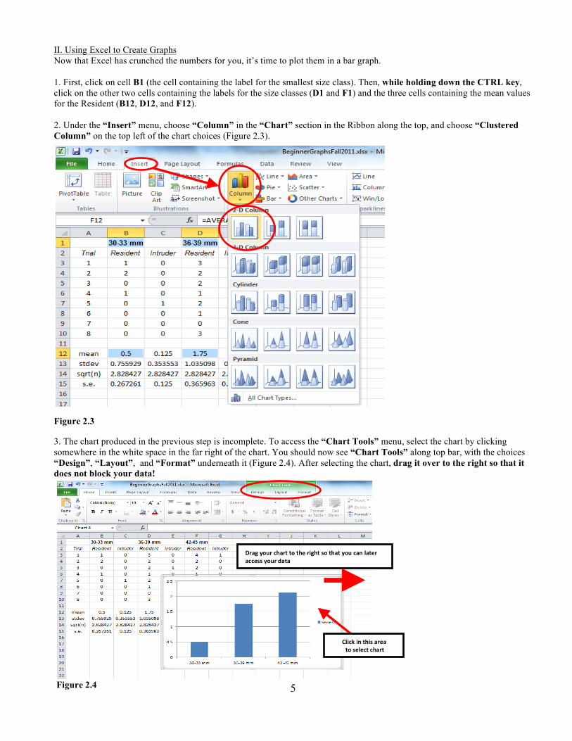
II. Using Excel to Create Graphs Now that Excel has crunched the numbers for you, it’s time to plot them in a bar graph. 1. First, click on cell B1 (the cell containing the label for the smallest size class). Then, while holding down the CTRL key, click on the other two cells containing the labels for the size classes (D1 and F1) and the three cells containing the mean values for the Resident (B12, D12, and F12). 2. Under the “Insert” menu, choose “Column” in the “Chart” section in the Ribbon along the top, and choose “Clustered Column” on the top left of the chart choices (Figure 2.3).

Figure 2.3

3. The chart produced in the previous step is incomplete. To access the “Chart Tools” menu, select the chart by clicking somewhere in the white space in the far right of the chart. You should now see “Chart Tools” along top bar, with the choices “Design”, “Layout”, and “Format” underneath it (Figure 2.4). After selecting the chart, drag it over to the right so that it does not block your data!

Figure 2.4

Drag  your  chart  to  the  right  so  that  you  can  later  access  your  data

Click  in  this  area  to  select  chart

6

1

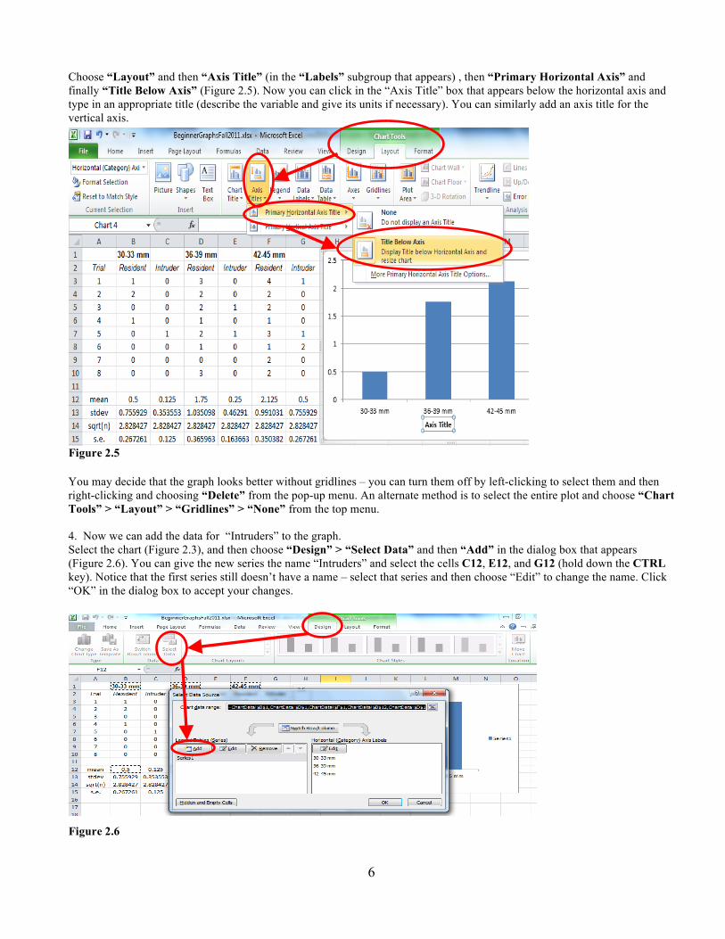
Choose “Layout” and then “Axis Title” (in the “Labels” subgroup that appears) , then “Primary Horizontal Axis” and finally “Title Below Axis” (Figure 2.5). Now you can click in the “Axis Title” box that appears below the horizontal axis and type in an appropriate title (describe the variable and give its units if necessary). You can similarly add an axis title for the vertical axis.

You may decide that the graph looks better without gridlines – you can turn them off by left-clicking to select them and then right-clicking and choosing “Delete” from the pop-up menu. An alternate method is to select the entire plot and choose “Chart Tools” > “Layout” > “Gridlines” > “None” from the top menu. 4. Now we can add the data for “Intruders” to the graph. Select the chart (Figure 2.3), and then choose “Design” > “Select Data” and then “Add” in the dialog box that appears (Figure 2.6). You can give the new series the name “Intruders” and select the cells C12, E12, and G12 (hold down the CTRL key). Notice that the first series still doesn’t have a name – select that series and then choose “Edit” to change the name. Click “OK” in the dialog box to accept your changes.

Figure 2.5

Figure 2.6

7

III. Adding Error Bars 1. Click once on one of the three bars corresponding to the “Residents” to select that data series – be sure to check that all

three bars of the “Resident” series are selected. 2. Choose “Chart Tools” > “Layout” > “Error Bars” > “More Error Bar Options” (Figure 2.7). Do NOT choose the

given “Standard Deviation” or “Standard Error” options – these lead to incorrect error bars!

Click OK in the intial “Add Error Bars” dialog box that may pop up - the “Format Error Bars” box should then appear (Figure 2.8).

Figure 2.7

3. IMPORTANT: you may need to uncover some of data that is being blocked by the “Format Error Bars” popup window (Figure 2.8).

Figure 2.8

The  “Format  Error  Bar”  dialog  box  may  be  blocking  some  of  your  data  –  move  it  first!  (click  on  the  title  bar  and  drag  it  to  the  right)

8

4. Click on the “Custom” toggle button at the bottom of the list of choices, then click on “Specify Values”. Be sure to delete the default entries (“={1}”) in the “Custom Error Bars” popup window before selecting your data! (Figure 2.9) For the “Resident” data series error bars, you will want to select cells B15, D15, and F15 (hold down the CTRL key while selecting). Click on the Close button when you have completed the task.

Figure 2.9

5. Repeat steps 1-4 for the “Intruder” data series, selecting cells C15, E15, and G15. Hint: if your error bars all appear to be the exact same size, it is probable that you have incorrectly added your error bars!

IV. Fine-Tuning Your Graph With Excel, you have control over virtually all aspects of chart appearance. Experiment by left-clicking on the various chart components (legend, x-axis, y-axis, data series, y-error bars, etc.), and then right-clicking to bring up a popup menu of choices for changing fonts and font sizes, fill and background colors, etc. You can also experiment with re-sizing and re-proportioning your graph by clicking once on the plot frame and dragging the square “handles” around the edges. Experiment and make changes until you are happy with your graph. But don’t go too wild! The best graphs are clean, simple, easy to interpret, and effective. You can also move your chart to its own worksheet by choosing “Chart Tools > “Design” and then “Move Chart Location” (far right of the “Design” ribbon that appears). When you are happy with your final graph, save your workbook! You can then select, copy, and paste the chart into Word or other word processing applications. One possibility for a final, finished graph, with an appropriate and concise figure legend appears in Figure 2.10 below.

Note: Color is nice, but if your chart must appear in black & white, use fill patterns to distinguish data series. Click on the series bars (or legend), and choose “Chart Tools”>“Format”>“Shape Fill”> “Gradient”>“More Gradients”>“Fill”>“Pattern Fill” to use fill patterns. Alternate method: right-click on data series and choose from the popup menu: “Format Data Series”>“Fill”>“Pattern Fill”

Figure 2.10. Mean number of ATR (all trunk raised) postures per 20-minute trial for resident and intruder Mountain Dusky Salamander (Desmognathus ochrophaeus) in the three separate size classes (n=8 each class). Error bars represent the standard error of the mean.

0  1  2  3  

30-­‐33  mm  

36-­‐39  mm  

42-­‐45  mm  

Freq

uency  of  ATR

 posture  

Size  Class  

Residents  

Intruders  

Delete  the  default  entries  in  the  “Custom  Error  Bars”  window  before  selecting  your  data!

0  

0.5  

1  

1.5  

2  

2.5  

3  

30-­‐33  mm   36-­‐39  mm   42-­‐45  mm  

Freq

uency  of  ATR

 posture  

Size  Class  

Residents  

Intruders  

9

3. EXCEL TUTORIAL: X-Y SCATTER PLOTS I. ENTERING DATA You can enter numbers anywhere in the worksheet that you like. However, you might want to be somewhat traditional and have the numbers that you want to graph near to each other. In the first cell of each column you can give a title to the data. Use the first column for your independent variable (x axis) data and the second column for your dependent variable (y axis) data. You can then enter the data into the columns. Here is some sample data for you to plot: Mass (kg) Food consumed (kcal)

1.5 42.6 2.7 98.4

10.1 340.8 21.6 716.4 47.8 1595.3 72.5 2625.2

II. PLOTTING DATA Once you have entered your data, you can make your graph. Choose “Insert” and then “Scatter” in the “Charts” submenu that appears, and then the simple X-Y scatter option (upper left from the choices) (Figure 3.1).

If your new (blank) chart isn’t already selected, then select it by left-clicking it (Figure 3.2 next page). You should see a “Chart” menu appear on the top bar with three suboptions “Design”, “Layout, “ and “Format” underneath it. Now select your data by choosing “Design” and then “Select Data” in the “Data” subsection that appears, and then “Add” in the popup dialog box (Figure 3.2 next page). In the “Edit Series” window that appears, you can select cell B1 for your series name and cells A2 to A7 for your X-values. You will need to delete the default (“={1}”) entry in the “Series Y values” box before selecting your Y-values (Figure 3.3 next page). Select cells B2 to B7 for the Y-values and click on “OK” to close the dialog boxes. Because we will have only one series for this chart, the “series legend” that appears on the right of the chart is not necessary and can be easily removed by selecting it and hitting the “delete” key. For graphs intended for publication, you will generally not want a title, so you click on the title that Excel provides and delete it as well. For graphs intended for a slide show, you may want to include a meaningful title; you can easily modify the default title by clicking in it and changing the text. In additon, the default chart comes with gridlines, but you can easily remove them by clicking and deleting them.

10

Click  the  chart  in  a  blank  area  to  select  it

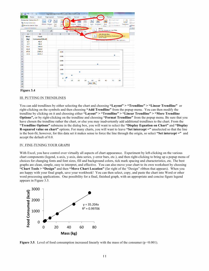
You can change other chart elements by selecting them (left-clicking on them), and then either choosing the appropriate menu from the top, or by right-clicking and choosing items from a popup menu that appears. For example, you need to provide axis labels describing your variables and units. Choose “Layout” and then “Axis Title” (in the “Labels” subgroup that appears) , then “Primary Horizontal Axis” and finally “Title Below Axis” (see Figure 3.4 next page). Now you can click in the “Axis Title” box that appears below the horizontal axis and type in an appropriate title (describe the variable and give its units if necessary). You can similarly add an axis title for the vertical axis – “Rotated title” is often a good choice. You can modify the appearance of the symbols by right-clicking on them, and then choosing “Format Data Series” at the bottom of the popup menu that appears. Note that fill color options are found under “Marker Fill”, but outline color options are found under “Marker Line Color”.

Figure 3.2

Figure 3.3

Be  sure  to  delete  the  default  entry  in  the  “Series  Y  values”  box  before  selecting  your  y-­‐values!

11

III. PUTTING IN TRENDLINES

You can add trendlines by either selecting the chart and choosing “Layout” > “Trendline” > “Linear Trendline” or right-clicking on the symbols and then choosing “Add Trendline” from the popup menu. You can then modify the trendline by clicking on it and choosing either “Layout” > “Trendline” > “Linear Trendline” > “More Trendline Options”, or by right-clicking on the trendline and choosing “Format Trendline” from the popup menu. Be sure that you have chosen the trendline rather the chart, or else you may inadvertently add additional trendlines to the chart. From the “Trendline Options” submenu in the dialog box, you will want to select the “Display Equation on Chart” and “Display R-squared value on chart” options. For many charts, you will want to leave “Set intercept =” unselected so that the line is the best-fit; however, for this data set it makes sense to force the line through the origin, so select “Set intercept =” and accept the default of 0.0. IV. FINE-TUNING YOUR GRAPH With Excel, you have control over virtually all aspects of chart appearance. Experiment by left-clicking on the various chart components (legend, x-axis, y-axis, data series, y-error bars, etc.), and then right-clicking to bring up a popup menu of choices for changing fonts and font sizes, fill and background colors, tick mark spacing and characteristics, etc. The best graphs are clean, simple, easy to interpret, and effective. You can also move your chart to its own worksheet by choosing “Chart Tools > “Design” and then “Move Chart Location” (far right of the “Design” ribbon that appears). When you are happy with your final graph, save your workbook! You can then select, copy, and paste the chart into Word or other word processing applications. One possibility for a final, finished graph, with an appropriate and concise figure legend appears in Figure 3.5.

Figure 3.5. Level of food consumption increased linearly with the mass of the consumer (p <0.001).

y  =  35.204x  R²  =  0.99706  

0  

1000  

2000  

3000  

0   20   40   60   80  Food

 Con

sumed

 (kcal)  

Mass  (kg)  

Figure 3.4

12

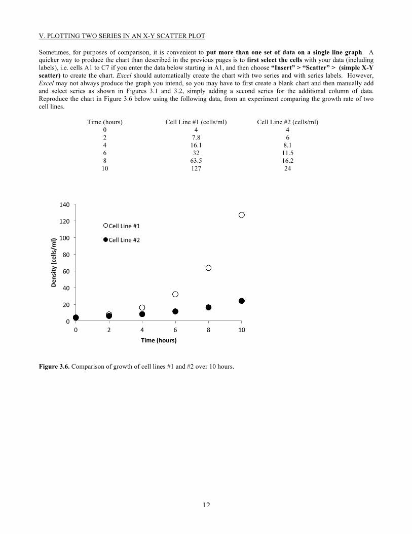
V. PLOTTING TWO SERIES IN AN X-Y SCATTER PLOT Sometimes, for purposes of comparison, it is convenient to put more than one set of data on a single line graph. A quicker way to produce the chart than described in the previous pages is to first select the cells with your data (including labels), i.e. cells A1 to C7 if you enter the data below starting in A1, and then choose “Insert” > “Scatter” > (simple X-Y scatter) to create the chart. Excel should automatically create the chart with two series and with series labels. However, Excel may not always produce the graph you intend, so you may have to first create a blank chart and then manually add and select series as shown in Figures 3.1 and 3.2, simply adding a second series for the additional column of data. Reproduce the chart in Figure 3.6 below using the following data, from an experiment comparing the growth rate of two cell lines.

Time (hours) Cell Line #1 (cells/ml) Cell Line #2 (cells/ml)

0 4 4 2 7.8 6 4 16.1 8.1 6 32 11.5 8 63.5 16.2

10 127 24

Figure 3.6. Comparison of growth of cell lines #1 and #2 over 10 hours.

0  

20  

40  

60  

80  

100  

120  

140  

0   2   4   6   8   10  

Density

 (cells/m

l)  

Time  (hours)  

Cell  Line  #1  

Cell  Line  #2