You Can’t Always Get What You Want:

The Impact of the UK Jobseeker’s Allowance

Alan Manning Centre for Economic Performance

London School of Economics Houghton Street

London WC2A 2AE

June 2005

Abstract In 1996 the UK made major changes to its welfare system for the support of the unemployed with the introduction of the Jobseeker’s Allowance. This tightened the work search requirements needed for eligibility for benefit. It resulted in large flows out of claimant status, but, this paper concludes, not into employment. The movement out of claimant status was largest for those with low levels of search activity. But, this paper finds no evidence of increased job search activity as a result of this change. Keywords: Unemployment Insurance, Job Search, Labour Supply JEL Classification: J64 I would like to thank Olivier Marie for his help in pointing me to data sources for this project and to seminar participants at CEP, MIT, Berkeley and McMaster for their comments. Equation Chapter 1 Section 1

1

Introduction

Most systems of welfare support for the unemployed make receipt of benefit

conditional on the individual making efforts to seek work, to be available for work

and not to impose unreasonable restrictions on the type of work they accept – what

are collectively known as eligibility conditions. Grubb (2000) provides an overview

of different OECD countries regulations of this type and argues that “the enforcement

of eligibility criteria may have a larger impact on behaviour than variations in

replacement rates…because the income implications for the individual are larger”

(Grubb, 2000, p149), although discussions of the incentive effects of UI systems tend

to focus on the level and duration of benefits.

This paper is about the impact of a major change to the UK system of welfare

support for the unemployed in October 1996 – the introduction of the Jobseeker’s

Allowance (JSA). This change had a large number of elements (described in more

detail below) but the most important aspect was a stricter enforcement of eligibility

conditions. Indeed the name change from the previous Unemployment Benefit

suggests the new emphasis on this welfare benefit being an allowance for those who

are looking for work instead of an income for those who are unemployed (that they

have a right to because of previous social security contributions they have paid).

In the UK, JSA is widely believed to have been a ‘big deal’. The reason for

this can be understood from a few pictures. Figure 1 presents the time series on the

UK claimant count for the period 1984-2004. JSA was introduced at a time when the

claimant count was falling but the months following introduction show a markedly

higher rate of decline. The fall in the seasonally adjusted claimant count in November

1996 was the highest ever recorded (Sweeney and McMahon, 1998). The reduction

2

in the claimant count seems primarily to have been due to an increased off-flow rather

than a reduced on-flow as can be seen from Figure 2.

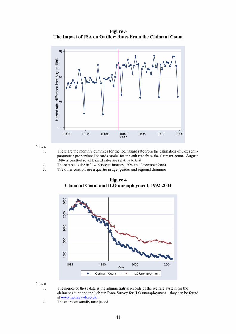
This is impressionistic evidence but more formal econometric evidence for an

increase in the outflow rate from the claimant count is strong. To make this point I

used the JUVOS dataset, a 5% random sample of claimants that contains information

of start and end dates as well as crude demographic characteristics (gender, age and

region). I estimated a model of the exit rate from the claimant count using a Cox

semi-parametric proportional hazard model with the baseline hazard being a function

of some demographics and separate dummies for each month. The coefficients on

these month dummies are plotted in Figure 3, where the vertical line marks the

introduction of JSA. There is clear evidence that the exit rate is higher after JSA than

before (the standard error on an individual monthly estimate is about 0.044 so these

differences are very significant). The estimate of a model of these month dummies on

a polynomial in time (to capture trends in the outflow rate), month dummies and a

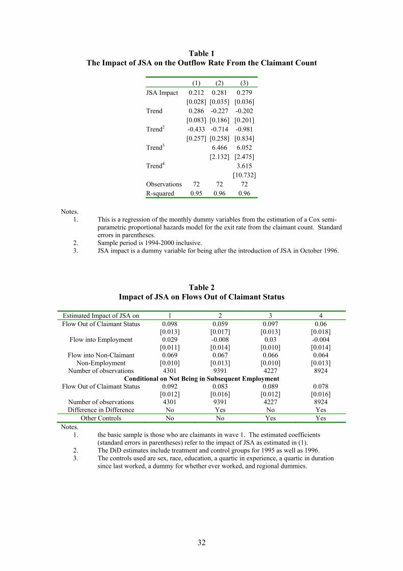
post-JSA dummy is reported in Table 1. According to these estimate the introduction

of JSA raised exit rates from the claimant count by between 21% and 28%, a very

large impact.

It does seem that JSA had an impact on the claimant count but did it also have

the other intended effects notably to encourage greater search activity among the

unemployed that, presumably, leads to higher flows into employment? It is widely

believed that it did. The research commissioned by the UK government into the

impact of JSA – see Trickey et al (1998), McKay et al (1999), Rayner et al, (2000),

and Smith et al (2000) - is voluminous but a good summary is “the initial increase in

movements off benefit was due to a ‘weeding out’ of those who were not previously

assiduous in their job search or were claiming fraudulently; and secondly, a stepping-

3

up of job search efforts on the part of jobseekers leading to more successful rates of

movement off benefit in the period immediately after the introduction of JSA”

(Rayner et al 2000, p1).

Unfortunately the research design used in this ‘evaluation’ has limitations.

The precise reasons for this are described below but it primarily consisted of a

comparison of two cohorts of claimants – one taken before JSA and one taken after.

This research design is unable to take account of the changing composition of the

claimant count if JSA weeded out those with low search intensity and unable to

consider the fate of those who were moved off the claimant count. If all those leaving

the claimant count went into employment that might not be such a deficiency but

there is evidence to suggest that many of those removed from the claimant count

remained non-employed. Figure 4 presents a comparison of the claimant count with

the numbers who are unemployed on the ILO definition (looked for work in the past 4

weeks and available to start work within 2 weeks). Prior to JSA these two series

tracked each other very closely (though there were always some claimants who were

not ILO unemployed and vice versa) but after JSA there is a remarkable divergence

that has never disappeared. This suggests that JSA removed some claimants who

were and remained unemployed on the ILO definition, perhaps suggesting that the

eligibility conditions under JSA were stricter than those implied by the ILO definition

of unemployment. Information on the destination of claimants leaving the count are

also recorded, albeit somewhat imperfectly. Figure 4 plots the proportion of exits to

employment, to inactivity (which includes sickness and disability benefits, retirement,

training and education and death) and to an unknown destination. There is no

evidence of a rise in the proportion of exits to employment after JSA and it also

4

suggests that a rising proportion of those leaving the claimant count were to

destinations unknown1.

The plan of this paper is as follows. The next section discusses related

literature and how this paper makes a contribution to it. The second section then

discusses the changes to the welfare system associated with the introduction of JSA.

The third section discusses the existing evaluation of JSA, arguing that some (though

not all) of the conclusions drawn are not really justified on the basis of the analysis

done. The fourth section discusses what economic theory has to say about the impact

of stricter eligibility conditions making the simple (but perhaps surprising point) that

those who are moved off welfare as a result of these rules may actually choose to

reduce their search activity. The fifth section discusses the data used in this paper and

reproduces the results obtained in the existing evaluation when using its methodology.

The sixth section then proposes a different methodology to get a better estimate of the

impact of JSA that avoids the problems identified in the existing evaluation. It shows

that JSA did have a sizeable impact on the flows out of claimant status but that this

flow was all into non-claimant non-employment and that this impact was larger for

those with low initial levels of job search activity – this is the ‘weeding-out’ effect.

The seventh section shows, however that the best estimate of the ‘average’ treatment

effect on search activity is very close to zero. The eighth section then investigates

whether there is any impact on the distribution of search activity but none is found.

The bottom line is that there is no evidence here that JSA had any impact on the

behaviour of any of the non-employed even though it did have a sizeable ‘weeding-

out’ effect.

1 See also Machin and Marie (2004) for evidence that JSA led to increases in crime. These extra crimes are not necessarily committed by the non-employed so this does not necessarily imply anything about employment destinations but it is suggestive that some of those leaving JSA are taking desparate measures.

5

1. Relationship to Existing Literature

There are a number of strands of existing literature related to the subject

matter of this paper.

First, there is a sizeable literature on the impact of stricter eligibility

requirements in UI systems and one might wonder what this study contributes to that

literature. This is an especially pertinent question as many of these studies use

randomised trials so might be thought to be higher quality than any analysis of JSA

(that was a non-experimental nationwide change) could possibly hope to be. Most of

the evidence from randomised trials comes from the US. Often these experiments

mix job search assistance with work search requirements so that there is a

combination of carrots and sticks involved. Meyer (1995) provides a very useful

review of the early studies and more recent ones can be found in Klepinger et al

(1997), Ashenfelter et al (1998), Black et al (2003). Typically these studies find that

increased job search assistance leads to modest but cost-effective reductions in UI

duration but the conclusions on the impact of stricter eligibility conditions seems

more mixed. Ashenfelter et al (1998) found little or no impact of tighter eligibility

checks on UI duration while Klepinger et al (1997) did find a modest impact of

requiring reporting of employer contacts. In the UK there is one randomized trial

(though others of recent policy initiatives are now under way) – that of the Restart

scheme that was introduced in 1989 (see Dolton and O’Neill, 1995, 1996, 2002, for

evaluation of this programme in various dimensions). In many ways this was a

precursor to JSA as it introduced the requirement of a compulsory eligibility check

after 12 months of unemployment (later reduced to 6 months).

6

Given the existence of randomized trials with similar interventions one might

wonder what is the contribution to knowledge that can be expected from studying JSA

as its introduction applied to everyone. There are several reasons for thinking that

there is useful information to be had from the study of JSA. First, findings from other

countries do not obviously generalise. Indeed, it will become apparent that all the

evidence suggests that the introduction of JSA resulted in larger numbers of

individuals moving off benefits so that the US studies that find little impact of stricter

eligibility checks would not seem to apply in the UK case – whether this is because

the UK requirements are now stricter or were laxer than the typical US system is

unclear.

Secondly, the study of a large change makes it possible to trace the impact

using national data sets rather than the specially constructed data sets commonly used

in the randomized trials. All of the randomized trials primarily report the impact of

the treatment on UI receipt and duration and, while this is of some independent

interest, one might also be interested in the destinations after leaving UI. The

motivation for many of the interventions is not just to move claimants off benefit to

reduce the burden on the public purse but also to move people from unemployment to

employment. A number of the studies give the impression that all those leaving UI

must be going into employment but there are some reasons to be sceptical abut this –

Figures 3 and 4 suggest this may not have happened with JSA. Many of the US

studies do report impacts on employment and earnings (tracking them through the

social security system) but it is very hard to know from these studies what fraction of

those leaving UI are actually ending up in employment. The evidence on JSA

presented below suggests that more attention should be paid to the destinations of

those leaving UI. Of course, how important this effect is likely to be depends on

7

whether the intervention under consideration is primarily a ‘carrot’ or a ‘stick’: while

JSA has aspects of both, the stick aspect seems the dominant one in practice.

Also relevant are the primarily Dutch studies of the impact of temporary

sanctions imposed on UI recipients for some violations of eligibility conditions With

the exception of van den Berg and van der Klaauw (2001) these are non-experimental

(see Abbring et al, 1997; van den Berg at al, 2004). Identification is achieved in these

models by the assumption that hazard rates have a mixed proportional form. These

studies find a very large effect of sanctions on the hazard rate both out of UI and into

employment, effects that seem to last much longer than the duration of the sanctions

themselves. These studies stand out as having results that are very different from the

ones found here.

The focus of this paper on search activity also means the paper has relevance

for the smaller literature that considers the impact of benefit receipt on job search

(see, for example, Blau and Robins, 1990, for the US, and Wadsworth, 1991, Schmitt

and Wadsworth, 1993, 2002, for the UK). These studies typically find that claimants

search more actively than non-claimants though a big problem with these studies is

the direction of the causality. Consideration of a change like JSA is helpful in

establishing whether the relationship is causal or not.

Finally this paper hopes to make a contribution to the literature on the

determination of search activity among the non-employed. As the definition of labour

market participation is based primarily on whether an individual searches for work,

this can be thought of as a contribution to the economics of labour supply. This

approach to labour supply has been taken before (see, for example, Burdett and

Mortensen, 1978, Burdett et al, 1984, Blundell at al, 1987, 1998) but the literature on

it is surprisingly small and one often comes away from that literature with the

8

impression that it is a nuisance to be controlled for when one is studying the important

aspect of labour supply - hours of work – rather than an important issue in itself.

2. What Is the Jobseeker’s Allowance?

JSA is the current system of welfare for those who are unemployed in the UK. It was

introduced on 7 October 1996 replacing the previous system of Unemployment

Benefit and Income Support (UB/IS). JSA comes in two forms. Contributory JSA

(known as contJSA) is a UI scheme with entitlement based on previous national

insurance contributions (as the UK social security payments are known) of limited

duration (6 months being the maximum), and not means-tested. This replaced the

previous UI scheme called Unemployment Benefit. Income-based JSA (known as

incJSA) is a UA scheme of potentially unlimited duration and potentially open to all

but means-tested. This replaced the previous UA scheme of Income Support. incJSA

is much more important with 85% of recipients of JSA getting that form in February

1997 and even among those with a duration of claim less than 6 months who are

potentially eligible for contJSA approximately 75% are receiving incJSA. The reason

for this is that many of the unemployed have insufficient National Insurance

contributions for entitlement to contJSA and the level of contJSA is quite low with

payments being topped up through incJSA if, for example, there are dependents in the

claimant’s household.

But the change of JSA was not simply a change of name: there were

substantive changes. Like most welfare systems, JSA is very complicated (see

Poynter and Barnes, 1997, for a 400-page guide to JSA produced for claimants) and

there were many changes in the switch from UB/IS to JSA. But the most important

changes can classified into two main areas.

9

First there were changes to the duration and level of benefits in the move from

UB to contJSA. UB had been payable for a maximum duration of 12 months and this

was reduced to 6 and the level of UB had been 10% higher than the level of IS and

this differential was eliminated. But, because a relatively small proportion of

unemployed claimants received UB the impact of this was relatively modest – Figure

6 plots the average payments received across the introduction of JSA – there is no

very marked change.

Secondly (and, I will argue, more importantly) there were changes to the job

search requirements required for eligibility. All claimants had to agree and sign a

Jobseeker’s Agreement with the Employment Service Staff – a copy of one is

attached in Appendix A. This detailed the type of job being sought, when the

claimant was able to work, and what steps will be taken to identify and apply for jobs.

Claimants were required to keep a record of their job search activities and at

fortnightly interviews these records were checked against what had been detailed in

the agreement. Furthermore, Employment Service staff were given the power to

direct claimants to apply for certain jobs.2 All of this was backed up with a greater

threat of sanctions and disqualification though the actual size of the sanctions

themselves was relatively modest. It seems likely that the main means by which JSA

moved claimants off benefit was by introducing the extra administrative hurdle of the

Jobseeker’s Agreement as other studies report that simply sending a letter inviting a

UI recipient to an interview that is meant to be of assistance to them (see Black et al,

2003 for a US example and Dolton and O’Neill, 2002, for a UK example) is enough

to make a sizeable proportion ‘disappear’. 2 There is of course a question about their ability to force claimants to take jobs – see the website www.urban75.com/Action/Jsa/jsa2.html for entertaining and creative advice to claimants on how to subvert the efforts of the ES to get you a job including “If you get an interview be (un)imaginative. Ask employers which union represents their workforce and whether they would object to you joining it, or, if there isn't one, starting one up”.

10

The thinking behind JSA was not entirely new. There was a widespread

perception that in the very severe ‘Thatcher’ recession of the early 1980s, eligibility

checks had virtually disappeared as the caseload rose, the number of case-workers

was reduced and the benefit administration and employment service were separated.

But beginning in the mid 1980s there were increasing attempts to enforce existing and

strengthen eligibility conditions (see Schmitt and Wadsworth, 2002, for a list of all

the changes). For example the Restart scheme that started in 1986 increased the

monitoring of the job search activity of the long-term unemployed, first for those with

duration more than 12 months and later extended to those unemployed for more than

six months. Schmitt and Wadsworth (2002) argue that the fall in the proportion of the

male unemployed who are claimants were mostly caused by stricter eligibility

requirements3. But, although JSA can be seen as the continuation of an existing trend

it was much more radical in requiring an explicit statement of what job search would

be done and holding claimants to this. And, as has already been seen in Figures 1 and

2 there does indeed seem to have been a particularly large impact effect.

3. The Existing ‘Evaluation’ of the Impact of JSA

The UK government did make some attempt to do an evaluation of the impact of JSA.

But it did not choose to use a randomized trial that had been used to evaluate the

earlier Restart programme. Essentially, a `before and after’ approach was taken with

two cohorts of benefit claimants. The first cohort was drawn from those unemployed

in July 1995 (i.e. pre-JSA) who were interviewed in Autumn 1995, Spring 1996 and

Summer 1997. The second cohort was drawn from a post-JSA sample and

interviewed twice. The methodology for evaluating JSA was essentially a comparison

3 This is perhaps in contrast to the US where Blank and Card (1992) ascribe a similar trend to falling take-up.

11

of the behaviour of these two cohorts. There are a number of reports on this but the

findings are well-summarized by “the initial increase in movements off benefit was

due to a ‘weeding out’ of those who were not previously assiduous in their job search

or were claiming fraudulently; and secondly, a stepping-up of job search efforts on the

part of jobseekers leading to more successful rates of movement off benefit in the

period immediately after the introduction of JSA” (Rayner et al 2000, p1).

Unfortunately, the research design of this evaluation means that the foundation

of some of these conclusions is not as strong as might be hoped for. There are two

main problems. First, if JSA did have a ‘weeding-out’ effect and disproportionately

removed low search activity individuals from the claimant count (and the evidence

presented below suggests that it did) then the average level of search intensity among

those who remain will be higher purely because of the composition effect. The post-

JSA cohort will show more search activity than the pre-JSA cohort but this need not

represent any change in behaviour at all.

The second problem is that the research design gives no information on what

happens to the search activity of those who were removed from the claimant count by

JSA but did not go into employment – the evidence of Figure 4 suggests this is quite a

large group. A reading of the literature often gives the impression that the fate of this

group is of no concern, either because they are not searching for work (so cannot do

less and might do more) or because they are abusing the system through a fraudulent

claim. But a less perjorative view would see at least some of this group as simply

having a level of search activity insufficient to meet the tighter eligibility restrictions

(and Figure 4 suggests many are still unemployed on the ILO definition) without

labelling them as ‘cheats’ in any way. And, as the next section makes clear, we

12

would expect some impact on the search activity of those who are moved off the

claimant count.

4. A Simple Model of Search Activity

In this section we present a very simple model of search intensity to develop some

predictions about the likely impact of tighter eligibility conditions. The model is a

familiar one in the literature (e.g. see Barron and Mellow, 1979; Mortensen, 1986)

There is a distribution of wage offers f(w) that arrive at a certain rate, ( )u sλ

for the non-employed and ( )e sλ for the employed that can be influenced by the level

of search activity, s, that has costs ( )uc s for the non-employed and ( )ec s for the

employed. The non-employed get a flow income of b and have to choose the

reservation wage, r, and the search intensity s. The value function for being without a

job can be written as:

( ),max ( ) ( ) ( )u us r u ur

V b s V w V dF w c sβ λ = + − − ∫ (1)

where β is the discount factor. The employed are assumed to face an exogenous risk

of job loss δ so their value function can be written as:

( ) ( ) ( ) ( ) ( )max ( ) ( ) us e ew

V w w s V x V w dF x V V w c sβ λ δ = + − + − − ∫ (2)

and they also have to choose their search intensity. The optimal policies are derived

in Appendix B but the essence of the model can be captured in a simple diagram. If

we substitute out the optimal reservation wage as a function of b and search intensity

then the indifference curves in b-s space for the non-employed will be as drawn in

Figure 7. A rise in b always raises utility and it is non-monotonic in s as there is an

optimal search intensity. If income while unemployed is independent of search effort

then the optimal search effort can be read off from the point where the indifference

13

curves are horizontal. Figure 7 shows the optimal levels of search intensity for two

levels of b – s must be declining in b for the simple reason that higher b makes non-

employment more attractive relative to employment.

A constant b can be thought of as a welfare system for the unemployed that is

independent of search effort. But a simple representation of a welfare system with

eligibility checks is that the payment of benefits is conditional on search effort being

above a certain level. For simplicity assume that the required search effort is non-

stochastic and known with certainty - denote it by s*. The budget line facing an

individual non-employed person can be thought of as a low level of benefits (it could

be zero) if s<s* and a higher level of benefits if s>s* - this is represented in Figure 8.

Now consider how the individual’s search intensity varies with the strictness

of the eligibility requirement. If s* is very low then the individual will choose Ls and

the eligibility condition will not bind. If * Ls s= the eligibility constraint starts to bind

and further increases in it lead to one-for-one increases in search intensity. This goes

on until we reach the point s** where the individual is indifferent between searching

at s** (and receiving welfare benefits) and leaving claimant status. A further increase

in s* makes the individual think it is too onerous to meet the eligibility requirements

and search intensity falls back to Hs . Note that an increase in job search requirements

in this case has actually led to a fall in search activity and a move out of claimant

status. The relationship between the search activity of the individual and s* will be as

plotted in Figure 9.

This should make it clear that economic theory does suggest that there is

reason to be interested in the impact of tighter eligibility conditions on those who

leave the claimant count as a result. It is possible that the search activity of this group

actually falls. Such an effect is not inevitable – if, for example, one moves from a

14

system with no effective eligibility checks to one with strict ones then even those who

leave the claimant count will raise their search effort because the level of benefit has

fallen. A similar analysis could apply if the level of benefits paid for a given level of

s* is reduced: some individuals may leave the claimant count as a result and their

search activity may fall. In understanding these effects it is important to think of the

welfare system as a subsidy to job search and not just a payment to those without

work.

There are other possible ways in which the benefit system could affect search

intensity. The specification of the utility function in (1) assumes that the time and

money involved in search activity is separable from the utility from income. It is

possible that there are ‘perverse’ effects of benefits on job search if there are strong

enough income effects e.g. workers at subsistence level or who are liquidity-

constrained or for whom leisure is locally inferior may use part of an increase to

search harder for work (see, for example, Hamermesh, 1982; Ben-Horim and

Zuckerman, 1987, and van den Berg, 1990). Schmitt and Wadsworth (1993, 2002)

also suggest that not being in claimant status reduces access to the job-placement part

of the Employment Service so may reduce flows out of non-employment. There are

also models of the impact of sanctions paying particular attention to the stochastic

element of the eligibility conditions (see Boone et al, 2000, 2001), something that

probably adds both realism and complication to the model. If the level of s* is

stochastic then one would expect a smooth but still non-monotonic relationship

between s and the strength of the eligibility conditions.

What this section has suggested is that a complete evaluation of JSA must take

account of any impact on those who are moved out of claimant status and that the

impact on job search intensity may have a different sign for different people. The

15

theory suggests that those with very high search intensity may see no effect (the

eligibility conditions never bind), those with a lower level of search intensity may see

a rise to maintain their claimant status and some of those who move out of claimant

status may actually see falls in their search activity. Hence it is of some interest to

look not just at average treatment effects but the distributional effect as well. The

methodology described below is designed to be able to address these concerns.

5. Data

This paper uses a methodology that is designed to avoide the pitfalls of the

existing evaluation of JSA. It is not a research design that one would choose if one

was given the power to do so but, given the way in which JSA was implemented, it is

the best I have come up with.

The main data set used in this paper is the UK Labour Force Survey (LFS), an

address-based quarterly survey of approximately 60,000 households that is the basis

for most UK labour market statistics (broadly it is equivalent to the US Current

Population Survey though it is much more detailed). Each sampled address is

followed for 5 quarters so there is a limited panel element. As this is a representative

national sample no-one is going to go missing and the impact of JSA is large enough

to be statistically detectable.

In addition to the usual demographic and labour market activity variables

(descriptive statistics on which can be found in Appendix C, Table C1), the LFS has

information on whether the individual is claiming unemployment-related benefits and

on search activity: these questions form the basis for the analysis. All those without a

job are asked whether they have searched for work in the past week and in the past 4

weeks (the latter information being used as part of the definition for ILO

16

unemployment). Those who do not report looking for work in the past four months

are then asked “even though you were not looking for work in the four weeks ending

Sunday, would you like to have a regular paid job at the moment” – using this

question one can divide the non-searchers into two categories – those who do not

want work and those who do4. Of course, one might wonder what exactly it means to

want work in an abstract sense but not search for it but, in practice, those who report

they do want work are more likely to enter employment than those who do not want

work even though neither group is recorded as searching for work in the past 4 weeks

(see Flinn and Heckman, 1983; Jones and Riddell, for statistical attempts to

discriminate between these different labour market states). I think it is probably best

to think of those who want work but have not searched in the past 4 weeks as having a

low level of search activity (e.g. they might have searched 6 weeks ago) rather than

zero. I will refer to this four-category classification of search activity as search

intensity.

For those who have searched for work in the past 4 weeks, there are questions

about the search methods used. These can be analysed independently or a summary

measure such as the number of search methods computed. In practice these variables

are correlated with moves into employment (see Gregg and Wadsworth, 1996) so,

while they may not be perfect measures of search activity they do seem to capture

some important elements of it.

4 There are then supplementary questions on why there is no job search among those who would like a job – for claimants, 28% report caring responsibilities, 15% the belief that no job is available (the traditional discouraged worker), 13% that they are long-term sick or disabled, 12% that they are temporarily sick or injured, 7% that they are a student, 6% that they have not started looking yet and 18% give some other reason. Among those who say they do not want work but are claimants, 41% report caring responsibilities as the reason , 19% that they are long-term sick or disabled, 7% that they are temporarily sick or injured, 12% that they are a student, 5% that they are retired and 14% give some other reason.

17

A first purpose is to show, using this data, that one can mimic the ‘findings’ of

the JSA evaluation. Figure 10 presents a time-series on the proportion of claimants

who report having searched for work in the past 4 weeks and in the past week. The

vertical line marks the introduction of JSA. The ‘evaluation’ of JSA compared these

variables at two points in time, before and after the introduction of JSA. There seems

to be a noticeable increase in the fraction of claimants who report searching in the

past week/month after JSA. Figure 11 then presents a similar time-series for the

fraction of claimants who report they have not searched but do want a job and who do

not want a job. There is a noticeable fall in the proportions of claimants in these

categories after the introduction of JSA. Figure 12 reports the average number of

search methods used by claimants. Again there is a marked rise in the number around

the introduction of JSA. In the evaluation of JSA this type of evidence is interpreted

as supportive of the view that JSA succeeded in raising the search intensity of the

unemployed. But, it does not control for the compositional changes in the claimant

stock induced by JSA and it does not tell us anything about what is happening to those

who are moved off the claimant count. My way of dealing with these issues is

described in the next section.

6. Methodology

The methodology for estimating the impact of JSA is the following. For a

‘treatment’ group I use claimants in the period July to September 1996 inclusive.

When first observed (what will be referred to as wave 1) these individuals will be

subject to pre-JSA rules and their eligibility for benefits will be defined by the pre-

JSA rules. But, when they are next observed 3 months later (what will be called wave

2) they will be subject to JSA rules. Of course, any change in labour market

18

outcomes or behaviour over these 3 months cannot be ascribed simply to the impact

of JSA. So, as the ‘control group’; we use claimants in the period April to June 1996

inclusive: when these individuals are observed 3 months later in wave 2 they are still

in the pre-JSA stage. Of course one might wonder how good a control group this is

but, as Table C1 shows the distribution of observed characteristics including job

search activity is very similar in treatment and control groups so that it does not seem

too unreasonable to assume the distribution of unobserved characteristics is also

similar. This finding also helps to allay fears that there were widespread anticipatory

effects of the introduction of JSA on behaviour because, for example, that would

cause differences in wave 1 search intensity between treatment and control groups.

But the treatment and control groups cannot be similar in season and there might be

concerns that any differences in outcomes between treatment and control groups

simply reflect a normal seasonal pattern. To allay these fears I construct treatment

and control groups in the same way for 1995 (the ‘treatment’ group here is not

receiving a treatment) and use a difference-in-difference approach to estimate the

impact of JSA. In practice, in most of the paper I use a simple regression approach to

estimating these treatment effects so estimate equations of the form:

0 1 1996 2 3 1996*y D JSA JSA Dβ β β β= + + + (3)

where y is the outcome variable, 1996D is a dummy variable for coming from the year

1996, JSA is a dummy variable for being form the July-September group and

1996*JSA D is an interaction between the two. The coefficient on this last variable

represents the difference-in-difference estimate of the impact of JSA. Sometimes

extra regressors are also included in (3) though their inclusion or exclusion typically

makes little differences as would be expected given the evidence presented earlier that

the treatment and control groups have very similar characteristics.

19

Is There Evidence of a Treatment?

I start by presenting evidence that JSA did move people off benefits as was strongly

suggested by the evidence from administrative data presented in Figures 1 and 2.

Accordingly the dependent variable in (3) is whether the individual has stopped

claiming at wave 2. Estimates of the treatment effect are presented in Table 2. Four

estimates are presented – the straight comparison of treatment and control group for

1996 and the difference-in-difference estimator, both with and without controls for

individual characteristics.

Table 2 presents estimate off the impact of JSA on the flow of claimants out of

claimant status. These estimates for 1996 alone suggest 9.8% of claimants were

moved out of claimant status by JSA with the inclusion or exclusion of controls

making little difference: the difference-in-difference estimators suggesting a lower

figure of 6%. These are in line with both the ONS estimates of 5-10% (Sweeney and

McMahon, 1998) and almost exactly in line with the estimate of a 21-28% increase in

the hazard rate from the earlier analysis of administrative data summarized in Table

15. Of course, these increased exits could be going to one of two destinations –

employment or non-claimant non-employment. The next part of Table 2 presents

estimates of the flows to these two states. As one can see, the 1996 data alone

suggests a modest increase of 3 percentage points in the flow into employment but

this disappears in the difference-in-difference estimates suggesting it represents a

seasonal effect and not the true impact of JSA. In contrast there remains a large

estimated increase of about 6.7 percentage points in the flow from claimant status to

5 One can obtain this by using the formula that if approximately 69% of claimants remain in that state in the absence of JSA and this falls by 6% with the introduction of JSA then the proportional increase in the hazard is ln(ln(0.69-0.06)/ln(0.69))=0.22.

20

non-claimant non-employed – this is consistent with Figure 4. So, JSA did increase

the exit rates from the claimant count but did not increase the flows into employment.

In what follows the sample used for estimation is often constructed as those

who were initially claimants but who had not exited to employment because search

activity is not observed for those who are subsequently employed. There is clearly a

selection issue involved in doing this but, given that the employment effect seems to

be very small, this does not seem to be important in practice. Table C2 also shows

that the treatment and control groups remain balanced when the sample is restricted in

this way. The bottom panel of Table 2 shows the estimated impact of JSA on flows

out of claimant status when the sample is constructed in this way – the estimates

suggest that JSA increased the flow out of claimant status by 8 to 9 percentage points.

Table 2 investigated the impact of JSA on flows out of claimant status. But it

is also possible that JSA had an impact on flows into claimant status. Table 3

presents a similar exercise for those who were non-employed non-claimants at wave 1

and Table 4 for those who were employed at wave 1. The estimated impacts of JSA

are all very small suggesting small impacts on the inflow. This is in line with Figure

2 that suggested that most of the impact was on out-flows. Given this, the rest of the

paper focuses on those who were claimants at wave 1.

As described above JSA had two main aspects: a reduction in potential

benefits for claimants with less than 12 months duration and stricter enforcement of

the eligibility conditions. So, one might expect that the impact on outflows depends

on the characteristics of the claimants. Tables 5 to 7 investigate this. Table 5

interacts the JSA dummy with the four levels of search intensity at wave 1: those who

have searched in the past week, those who searched only in the past 4 weeks, those

who want a job but have not searched in the past 4 weeks and those who do not want

21

a job. The first column shows that those who have searched in the past week are less

likely to be moved off claimant status by JSA than those who want a job but have not

searched in the past week. There is a slight anomaly in that those who do not want

work seem to have the smallest impact of JSA but the difference-in-difference

estimates of the JSA impact for this group are large suggesting this is a seasonal

effect. It should be noted however that there is a significant estimated impact of JSA

on those who have searched in the past week even though the impact is larger for

those with lower initial levels of search intensity6.

Table 6 does the same exercise but using the number of search methods in

wave 1 as the measure of search activity. The estimated impact of JSA is larger for

those who report lower numbers of search methods in wave 1. So, both Tables 5 and

6 suggest that JSA had a ‘weeding-out’ effect as the existing evaluation concluded,

disproportionately removing from he claimant count those with low levels of search

activity.

Finally Table 7 investigates the importance of the duration of claim by

including controls for those with less than 12 months duration of claim (who were

potentially affected by the benefit reductions). The reported coefficients are the extra

treatment effect for this group. The coefficient of –0.045 in the first column of the

first row of Table 7 suggests that short-duration claimants were less likely to be

moved off claimant status than long duration claimants, the opposite of what would be

expected to happen if the benefit reductions were the most important aspect of JSA.

The second and third rows of Table 7 shows that this effect gets larger if one also

controls for the differential impact of JSA according to the level of wave 1 search

activity, either search intensity (the second row) or the number of search methods (the

6 It should be remembered that this is reported search activity prior to JSA so the intensity might change over time.

22

third row). This suggests the main impact of JSA was from the tighter eligibility

conditions and not from the benefit reductions. This is consistent with the fact that

the benefit reductions seem to have been small (see Figure 6).

So, JSA does seem to have increased the flows out of claimant status,

primarily (and maybe totally) into non-claimant non-employment. The impact is

estimated to be larger for those who initially reported low levels of search activity so

JSA did have the intended ‘weeding-out’ effect. But, what were the impacts on

search behaviour? – this is the subject of the next section.

7. The Impact of JSA on Job Search Activity: Average Treatment Effects

The previous section demonstrated that one way to lessen the impact of JSA

was to be searching intensively and using a large number of different search methods.

Given this one might expect that the incentives to search were increased by JSA (as

was its intention) and one should be able to see this in the reported levels of search

activity.

Table 8 investigates this using the two different measures of search activity.

The first row reports the results where the measure of search activity is the four-fold

categorization of search intensity. This is estimated using an ordered probit so the

four categories can be reduced to one dimension (later estimates look at the four

categories separately). The reported coefficients are the index in the ordered probit

model. The estimated treatment effects are tiny and insignificantly different from

zero. The second row does the same exercise but with the number of search methods

as the dependent variable. Again the estimated treatment effects are tiny and

insignificantly different from zero. There is no evidence here that JSA had any

impact on reported job search activity.

23

How can this be reconciled with the graphical evidence presented in Figures

10-12. The answer is that JSA did disproportionately remove from the claimant count

those with low levels of search activity – the changing composition of the claimant

count then could account for some or all of the apparent increase in job search activity

among claimants. One can see this by attempting to estimate the impact of JSA on

search activity using wave 2 claimants as the sample – not wave 1 claimant status.

This is a similar exercise to that which was done in the official evaluation of JSA.

The second panel of Table 8 shows that this leads both to large estimated ‘treatment’

effects that are significantly different from zero. And these results are obtained using

only one quarter pre- and post-JSA: precision would be much greater if more quarters

were included. However, it should be emphasized that these ‘treatment’ effects are

spurious.

A simple way of illustrating the difference between the true and ‘spurious’

treatment effects is contained in Table 9. In the top panel the outcome measure is the

proportion searching in the past week at wave 2 and in the bottom panel it is the

average number of search methods used. We report these outcome measures for those

who remain claimants at wave 2, those who become non-employed non-claimants and

for both groups together. The ‘spurious’ treatment effect can be found by comparing

the outcomes of treatment and control groups for those who remain claimants. Both

outcomes show an increase in search activity. If one compares the outcomes for wave

2 non-claimants one also finds increase in search activity, with a very large effect.

But these apparent treatment effects are driven entirely by the changes in composition

of the claimant stock as a result of the ‘weeding-out’. The row labelled ‘all’ shows

the true treatment effect and this is zero.

24

There are two possible explanations for the finding of zero average treatment

effects. One is that there really is no effect on anyone, the other that there is an

impact on the distribution of search effort with those who remain claimants increasing

their search activity at the same time as those who leave the claimant count are

perhaps reducing theirs as the theory presented above suggested. The next section

investigates distributional effects.

8. The Impact of JSA on Job Search Activity: The Distribution of Treatment

Effects

This section investigates whether there is any impact of JSA on the

distribution of job search activity. The theory presented in the fourth section

suggested that there might be both an increase in the numbers reporting high levels of

search activity and a low level of search activity. This obviously has the ability to

explain why the average treatment effect is essentially zero at the same time as JSA

still had an impact on search activity.

There are a number of ways in which one might hope to detect any

distributional effect. The first is to consider directly the impact of JSA on the

distribution of search activity with no other conditioning variables. The second is to

take advantage of the fact that the theory predicts different impacts on those with

different levels of search activity. Of course, we do not observed what search activity

would have been in the absence of JSA but because job search activity is correlated

over time (something that can be verified from an analysis of the control groups) one

can look for different treatment effects by differing levels of wave 1 search activity.

Finally the theory suggested different treatment effects for those who remain in and

those who are moved out of claimant status with positive impacts for the former and

25

possibly negative effects for the latter. So, a third strategy is to try to estimate

average treatment effects for these two groups. All of these strategies are tried in

what follows.

The Unconditional Distribution

For the search intensity variable there are only four categories so that the

distributional impact can be summarized by estimating the impact of JSA on the

proportions of workers in those four categories. These estimates are presented in

Table 10. There is perhaps a little bit of evidence that there is a rise in the proportion

who don’t work at the expense of the proportions in the next two categories but the

effects are small and insignificantly different from zero so there is not really any

evidence here that the introduction of JSA led to a widening dispersion of outcomes.

Turning to the number of search methods, Table 11 reports the estimates of the

impact of JSA on the proportion of workers reporting different number of search

methods. Again there seems to be no impact at any point in the distribution.

There is no evidence here that the zero average treatment effect is hiding a

widening dispersion but perhaps this has low power because one would expect very

little impact on the overall distribution.

The Conditional Distribution

The theory presented in section 4 suggested that the impact of JSA might vary

according to what the level of job search activity would be in the absence of JSA with

zero effect for those with the highest search activity, positive effects for those in the

middle and possibly negative effects for those at the bottom. Of course, the search

activity in the absence of JSA is not observed but, because the most powerful

26

predictor of future search intensity is current search intensity one way of looking at

the conditional distribution is to estimate the average treatment effects for those with

a different level of search intensity in wave 1. The paper has already shown that those

with low levels of search intensity in wave 1 are more likely to be moved off the

claimant count by JSA. This is done for search intensity in Table 11 and the number

of search methods in Table 12. There is no evidence here of any distributional

effects.

The Treatment Effect for Stayers and Movers

The theory suggested that the treatment effect for those who remain in claimant status

(call this group the stayers) should be positive while for those who move out of

claimant status (call this group the movers) it could be negative. This suggests trying

to estimate separate treatment effects for these two groups.

Suppose we are interested in some outcome variable y with a distribution

function G(y)7. The distribution of y for wave 2 claimants and non-claimants is

observed both pre-JSA (from the control group) and post-JSA (from the treatment

group). The notation used and the information available is summarized in Table 14.

In addition, one can observe the proportions in claimant and non-claimant status in the

treatment and control groups.

From this information we would like to be able to identify the different

treatment effects for the movers and the stayers. One can think of classifying

individuals by what their wave 2 claimant status would be under the pre-JSA and

post-JSA regimes – this is a version of the full-outcomes approach used by Angrist

7 The discussion of identification is phrased in terms of the identification of the change in the distribution function because this is quite general and other statistics like mean treatment effects can be derived from it

27

and Imbens (1994). Denote by ijp the proportion of the population who would be in

state i (where i=C,N) under the pre-JSA regime and in state j under the post-JSA

regime. There are obviously 4 potential groups. For each of these groups denote by

( )0ijF y the distribution of y under the pre-JSA regime and by ( )1

ijF y the distribution

of y under the post-JSA regime. There are eight such distribution functions so one

cannot immediately identify the treatment effects for the different groups from the

four observed distribution functions in Table 14.

One can get some identifying assumptions if one takes the theory of job search

choice seriously. First, there are no individuals who would be non-claimants under

the pre-JSA regime and are claimants under the post-JSA regime. This amounts to

the restriction:

0NCp = (4)

This can be thought of as a version of the monotonicity assumption of Angrist and

Imbens (1994). This restriction allows us to estimate the other ijp from observations

on the proportion of claimants and non-claimants in pre- and post-JSA regimes. For

example, the excess of the proportion of non-claimants in the post-JSA regime over

the pre-JSA regime is the estimate of CNp , the proportion of claimants in the post-

JSA regime is the estimate of CCp , and the proportion of non-claimants in the pre-

JSA regime is the estimate of NNp .

The restriction in (4) also implies that ( )0NCF y and ( )1

NCF y are both

undefined and irrelevant because they refer to the behaviour of individuals who do not

exist. This gives two identifying assumptions on the distribution functions.

The theory also predicts that the behaviour of those who are non-claimants in

wave 2 in both regimes is the same under both regimes as the behaviour cannot be

28

influenced by a welfare system in which they do not participate. This amounts to the

identifying restriction:

0 1NN NNF F= (5)

But even with these identifying restrictions we are still one restriction short of

full identification. What can be identified in this case?: Appendix D shows that the

best that can be identified is the treatment effect for a weighted average of the movers

and stayers which is given by:

CN CN CC CC

CN CC CN CC

p F p F Gp p p p

∆ + ∆ ∆=

+ + (6)

where 1 0G G G∆ = − , 1 0CN CN CNF F F∆ = − , the treatment effect for movers and

1 0CC CC CCF F F∆ = − , the treatment effect for stayers. The numerator of the right-hand

side of (6) is the overall treatment effect that has been analysed earlier and was found

to be close to zero. (6) says that this overall treatment effect (divided by the fraction

of individuals for whom the treatment effect is non-zero) is a weighted average of the

treatment effects for movers and stayers. It should be apparent that (6) is consistent

with positive effects for the stayers and negative effects for the movers with the

weighted average of the two averaging out to the zero that is approximately the

overall treatment effect. Appendix D shows that the source of the inability to identify

the separate treatment effects for movers and stayers is the lack of information on

wave 2 claimants in the control group about who would be a mover and who a stayer

if treatment were applied.

There are a number of ways in which one might make progress. If one could

find an ‘instrument’ that affected the sample proportions in (6) but left the treatment

effects unchanged then one could use this to work out the treatment effects for movers

and stayers. However, anything that is likely to affect the proportion of movers and

29

stayers is also likely to affect the treatment effects e.g. more stringent eligibility

requirements are likely to mean a larger positive treatment effect for stayers and a

more negative one for movers.

Here, I take a less ambitious approach and seek to provide bounds for the

treatment effects. The finite nature of the outcome variables being considered helps

to provide bounds. To give an example of how this works, to get an upper bound for

the treatment for stayers we assign all those with low values of the outcome variable

among the wave 2 claimants in the control group to be stayers. This minimizes the

outcome variable for stayers in the control leading to an upper bound for the treatment

effect. The other side of this coin is a lower bound for the treatment effect for

movers. One can then apply the process in reverse to get an upper bound for the

movers and a lower bound for the stayers.

The results of this exercise are presented for two outcome variables in Table

15 – the proportion who have searched for work in the past week and the average

number of search methods. The 95% confidence intervals are computed using a

bootstrap with 1000 replications. The bounds are very large, especially for the

movers because they are a smaller fraction of the group. Because these bounds are (as

is quite common) too large to be useful, I also report some bounds based on more

‘intuitive’ restrictions.

To have very large positive treatment effects for the movers and large negative

effects for the stayers is somewhat implausible as it implies that it is the stayers who

had low levels of search intensity in the absence of treatment. A reasonable

restriction is that the distribution of search intensity among the stayers stochastically

dominates that for the movers in the absence of treatment i.e to impose a bound of the

form:

30

0 0CC CNF F≤ (7)

Appendix D then shows that this can then be used to put an upper bound on the

treatment effect for the stayers: of the form:

CC CF G∆ ≥ ∆ (8)

and a lower bound on the treatment effect for the movers of the form:

CC C

CNCN

G p GFp

∆ − ∆∆ ≤ (9)

To get the other bounds, I impose a lower bound on the treatment effect for

stayers of zero on the grounds that it is hard to believe that JSA reduced search

activity for those who remained claimants. This restriction, using (6), translates into

an upper bound on the treatment effect for movers of zero as well, given that the

overall change is zero.

Applying the intuitive bounds leads to the results in the second panel of Table

15. These are much smaller than the bounds obtained from the data restrictions alone.

Because of the lower bound of zero imposed on the treatment effect for stayers there

is little surprise that the bounds for stayers are non-negative but the bounds for the

movers now lie almost all in the non-positive region of the real line.

These bounds mean that the data is largely consistent with the view that the

treatment effect is positive for the stayers and negative for the movers but it must also

be admitted that it is also consistent with the view that it is zero for both groups

9. Conclusion

The introduction of JSA in the UK was a big deal – it seems to have reduced the

claimant count by about 8 percentage points. The impact was larger for those with

low levels of search activity. This obviously resulted in savings in the payment of

31

welfare benefits but it was also intended that the change increase the search activity of

jobseekers and, hence, raise inflows into employment. This paper has found no

evidence that moves into employment or measures of search activity were increased

by JSA and has argued that there serious problems with existing evidence on this

subject. However, this paper has not resolved all problems: it is not clear why there

was little or no behavioural response to a regime change that did tighten eligibility

conditions considerably.

There is something of a puzzle here: the results suggest that one way to

insulate oneself from the impact of JSA was to increase search intensity yet no

claimants seem to have done that. Rather, the implication of zero treatment effects is

that claimants accepted JSA in a fatalistic way. This might be because the

construction of the treatment and control groups used here inevitably only looks at

short-term impacts: perhaps the longer-term impacts were more positive. It is

difficult to provide a test of this in the absence of a good research design but there is

certainly no sign of a change in reported search activity among the non-employed

associated with the introduction of JSA. Figure 13 presents a time series on the

average number of search methods reported by the non-employed as a whole for the

period 1995-1998. The downward trend is primarily because the labour market

recovery is meaning that a higher proportion of the non-employed are those who are

not interested in paid.work. There is no noticeable break at the introduction of JSA.

Anyone who wanted to argue for a positive impact of JSA would have to argue that

the downward trend would have been even more marked in the absence of JSA: while

conceivable, this is hardly persuasive evidence.

So, the best that can be said is that the short-run effect of JSA on search

activity seems to have been negligible and the case for a longer-run impact unproven.

32

Table 1 The Impact of JSA on the Outflow Rate From the Claimant Count

(1) (2) (3) JSA Impact 0.212 0.281 0.279 [0.028] [0.035] [0.036] Trend 0.286 -0.227 -0.202 [0.083] [0.186] [0.201] Trend2 -0.433 -0.714 -0.981 [0.257] [0.258] [0.834] Trend3 6.466 6.052 [2.132] [2.475] Trend4 3.615 [10.732]Observations 72 72 72 R-squared 0.95 0.96 0.96

Notes.

1. This is a regression of the monthly dummy variables from the estimation of a Cox semi-parametric proportional hazards model for the exit rate from the claimant count. Standard errors in parentheses.

2. Sample period is 1994-2000 inclusive. 3. JSA impact is a dummy variable for being after the introduction of JSA in October 1996.

Table 2 Impact of JSA on Flows Out of Claimant Status

Estimated Impact of JSA on 1 2 3 4

0.098 0.059 0.097 0.06 Flow Out of Claimant Status [0.013] [0.017] [0.013] [0.018] 0.029 -0.008 0.03 -0.004 Flow into Employment

[0.011] [0.014] [0.010] [0.014] 0.069 0.067 0.066 0.064 Flow into Non-Claimant

Non-Employment [0.010] [0.013] [0.010] [0.013] Number of observations 4301 9391 4227 8924

Conditional on Not Being in Subsequent Employment 0.092 0.083 0.089 0.078 Flow Out of Claimant Status

[0.012] [0.016] [0.012] [0.016] Number of observations 4301 9391 4227 8924 Difference in Difference No Yes No Yes

Other Controls No No Yes Yes Notes.

1. the basic sample is those who are claimants in wave 1. The estimated coefficients (standard errors in parentheses) refer to the impact of JSA as estimated in (1).

2. The DiD estimates include treatment and control groups for 1995 as well as 1996. 3. The controls used are sex, race, education, a quartic in experience, a quartic in duration

since last worked, a dummy for whether ever worked, and regional dummies.

33

Table 3

Impact of JSA on Flows Into Claimant Status: Non-Claimant, Non-Employed

Estimated Impact of JSA on 1 2 3 4 0.014 -0.005 0.014 -0.004 Flow into Claimant Status

[0.003] [0.005] [0.003] [0.005] -0.008 0.008 -0.009 0.006 Flow into Employment [0.004] [0.005] [0.004] [0.005] -0.005 -0.003 -0.005 -0.002 Flow into Non-Claimant

Non-Employment [0.002] [0.003] [0.002] [0.003] Number of observations 23817 47812 23337 45886

Conditional on Not Being in Subsequent Employment -0.005 -0.003 -0.005 -0.002 Flow Out of Claimant Status [0.002] [0.003] [0.002] [0.003]

Number of observations 22127 44468 21674 42622 Difference in Difference No Yes No Yes

Other Controls No No Yes Yes Notes.

1. the basic sample is those who are non-employed but non-claimants in wave 1. The estimated coefficients (standard errors in parentheses) refer to the impact of JSA as estimated in (1).

2. The DiD estimates include treatment and control groups for 1995 as well as 1996. 3. The controls used are sex, race, education, a quartic in experience, a quartic in duration

since last worked, a dummy for whether ever worked, and regional dummies.

Table 4 Impact of JSA on Flows Into Claimant Status: Employed

Estimated Impact of JSA on 1 2 3 4

-0.0012 0 -0.0013 0 Flow into Claimant Status [0.0006] [0.0009] [0.0006] [0.0009] 0.0016 -0.0002 0.0017 0.0001 Flow into Employment

[0.0011] [0.0015] [0.0011] [0.0015] 0 0.0002 -0.0004 -0.0001 Flow into Non-Claimant

Non-Employment [0.001] [0.0012] [0.0009] [0.0012] Number of observations 90761 183192 90057 178963

Conditional on Not Being in Subsequent Employment -0.031 -0.008 -0.045 -0.022 Flow Out of Claimant Status [0.019] [0.027] [0.018] [0.025]

Number of observations 2342 4885 2320 4739 Difference in Difference No Yes No Yes

Other Controls No No Yes Yes

Notes. 1. the basic sample is those who are employed in wave 1. The estimated coefficients

(standard errors in parentheses) refer to the impact of JSA as estimated in (1). 2. The DiD estimates include treatment and control groups for 1995 as well as 1996. 3. The controls used are sex, race, education, a quartic in experience, a quartic in duration

since last worked, a dummy for whether ever worked, and regional dummies.

34

Table 5

Impact of JSA on Claimant Outflow by Wave 1 Search Intensity

Wave 1 Search Intensity 1 2 3 4 0.031 0.131 0.025 0.123 Don’t want work

[0.041] [0.038] [0.042] [0.040] 0.154 0.128 0.142 0.113 Want Work – no search

[0.036] [0.035] [0.037] [0.036] 0.189 0.157 0.203 0.169 Search in Past 4 weeks

[0.051] [0.046] [0.051] [0.047] 0.082 0.064 0.08 0.061 Search in Past week

[0.013] [0.016] [0.013] [0.016] Difference in Difference No Yes No Yes

Other Controls No No Yes Yes Observations 4301 9391 4227 8924

Notes. 1. The sample are the claimants used and is the same as in Table 2. Notes to that table apply here. The search intensity variables are interacted with all year and treatment dummies.

Table 6 Impact of JSA on Claimant Outflow by Wave 1 Number of Search Methods

No. of search methods in

wave 1 1 2 3 4

0.099 0.127 0.09 0.119 0 [0.028] [0.027] [0.028] [0.028]

0.114 0.148 0.111 0.118 1 [0.063] [0.058] [0.063] [0.064]

0.175 0.183 0.161 0.161 2 [0.046] [0.044] [0.047] [0.046]

0.126 0.093 0 0.084 3 [0.036] [0.034] [0.000] [0.035] 0.067 0.063 0.06 0.064 4

[0.032] [0.031] [0.032] [0.031] 0.071 0.035 0.08 0.043 5

[0.029] [0.029] [0.029] [0.029] 0.09 0.053 0.084 0.047 6

[0.028] [0.028] [0.027] [0.028] 0.056 0.035 0.058 0.038 7

[0.035] [0.035] [0.035] [0.035] 0.052 0.081 0.058 0.085 8+

[0.052] [0.051] [0.051] [0.050] Difference in Difference No Yes No Yes

Other Controls No No Yes Yes Observations 4301 9391 4227 8924

Notes. 1. The sample are the claimants used and is the same as in Table 2. Notes to that table apply here. The search intensity variables are interacted with all year and treatment dummies.

35

Table 7

Dffierential Impact of JSA on Claimant Outflow for Short-Duration Claimants

Other controls 1 2 3 4 -0.045 -0.052 -0.054 0.067 None

[0.027] [0.024] [0.027] [0.024] -0.065 -0.067 -0.070 -0.074 Wave 1 search

activity

[0.026] [0.023] [0.026] [0.023]

-0.062 -0.063 -0.066 -0.071 Wave 1 number of search methods

[0.026] [0.023] [0.026] [0.023]

Difference in Difference

No Yes No Yes

Other Controls No No Yes Yes Observations 4301 9391 4227 8924

Notes. 1. The sample are the wave 1 claimants as in Table 2. Notes to that table apply here. 2. The reported coefficients are those for the differential treatment effect on those with duration less than 12 months.

Table 8 Average Impact of JSA on Search Activity

Outcome Variable 1 2 3 4

‘True’ Treatment Effects -0.012 0.009 -0.018 0.018 Search Intensity [0.039] [0.053] [0.041] [0.056] -0.007 -0.007 -0.022 0.022 Number of Search

Methods [0.081] [0.109] [0.076] [0.105] Number of

observations 4301 9391 4227 8924

‘Spurious’ Treatment Effects 0.101 0.107 0.071 0.07 Search Intensity

[0.040] [0.053] [0.045] [0.061] 0.246 0.227 0.14 0.135 Number of Search

Methods [0.072] [0.097] [0.074] [0.101] Number of

observations 4794 10741 4007 8640

Difference in

Difference No Yes No Yes

Other Controls No No Yes Yes Notes. 1. The sample in the panel labelled ‘True Treatment Effects’ are the claimants used and is the same as in Table 2. Notes to that table apply here. 2. The sample in the panel labelled ‘Spurious Treatment Effects’ use as the sample those who are claimants at wave 2. For the treatment group this will be affected by JSA.

36

Table 9

Reconciling ‘True’ and ‘Spurious’ Treatment Effects

Control Group Treatment Group Proportion Search in Past Week at Wave 2

Wave 2 Claimant 0.812 (0.39)

0.838 (0.37)

Wave 2 Non-Claimant 0.310 (0.46)

0.424 (0.49)

All 0.734 (0.44)

0.736 (0.44)

Average Number of Search Methods in Wave 2 Wave 2 Claimant 4.39

(2.42) 4.54

(2.40) Wave 2 Non-Claimant 1.69

(2.59) 2.22

(2.65) All 3.97

(2.63) 3.97

(2.66) Sample Sizes

Wave 2 Claimant 339 521 Wave 2 Non-Claimant 1849 1591

All 2188 2112 Notes.

1. These relate to 1996 treatment and control groups only who are not in employment at wave 2. Standard errors in parentheses.

Table 10 The Impact of JSA on the Distribution of Search Intensity

Wave 2 Search

Intensity 1 2 3 4

0.012 0.011 0.01 0.006 Don’t want work [0.009] [0.012] [0.009] [0.012]

-0.01 -0.019 -0.008 -0.018 Want Work – no search [0.010] [0.013] [0.010] [0.013]

-0.004 -0.002 -0.004 -0.001 Search in Past 4 weeks [0.007] [0.009] [0.007] [0.010]

0.002 0.01 0.002 0.013 Search in Past week [0.013] [0.018] [0.013] [0.018]

Difference in Difference

No Yes No Yes

Other Controls No No Yes Yes Observations 4300 9390 4300 9390

Notes. 1. The sample are those who are claimants in wave 1 and is the same as in Table 2. Notes to that table apply here.

37

Table 11

Impact of JSA on Distribution of Search Methods

No. of search methods in wave

2

1 2 3 4

0.003 -0.006 0.002 -0.011 0 [0.012] [0.017] [0.012] [0.016]

0.002 0.004 0.005 0.006 1 [0.006] [0.007] [0.006] [0.007]

0.003 0.014 0.002 0.007 2 [0.007] [0.009] [0.007] [0.009]

-0.003 0.004 -0.003 0.006 3 [0.009] [0.012] [0.009] [0.012] -0.002 -0.011 -0.001 -0.009 4

[0.010] [0.013] [0.010] [0.014] -0.001 -0.004 -0.003 -0.001 5 [0.011] [0.015] [0.011] [0.015] -0.012 -0.018 -0.012 -0.015 6 [0.012] [0.015] [0.012] [0.016] 0.008 0.017 0.007 0.018 7

[0.010] [0.013] [0.010] [0.013] 0.004 -0.001 0.003 -0.002 8+

[0.007] [0.010] [0.007] [0.010] Difference in

Difference No Yes No Yes

Other Controls No No Yes Yes Observations 4301 9391 4227 8924

Notes. 1. The sample are those who are claimants in wave 1 and is the same as in Table 2. Notes to that table apply here.

Table 12 Treatment Effect by Wave 1 Level of Search Intensity

Wave 1 Search Intensity

1 2 3 4 Number of Obser-vations

-0.045 -0.033 -0.167 -0.171 329 Don’t want work

[0.141] [0.188] [0.164] [0.204]

0.153 0.118 0.222 0.208 430 Want Work – no search [0.110] [0.148] [0.117] [0.156]

-0.096 -0.071 -0.048 -0.143 217 Search in Past 4 weeks [0.151] [0.202] [0.171] [0.214]

-0.049 0.019 -0.062 0.017 3324 Search in Past week [0.055] [0.077] [0.057] [0.079]

Difference in Difference

No Yes No Yes

Other Controls

No No Yes Yes

Notes. 1. The sample are those who are claimants in wave 1 and is the same as in Table 2. Notes to that table apply here.

38

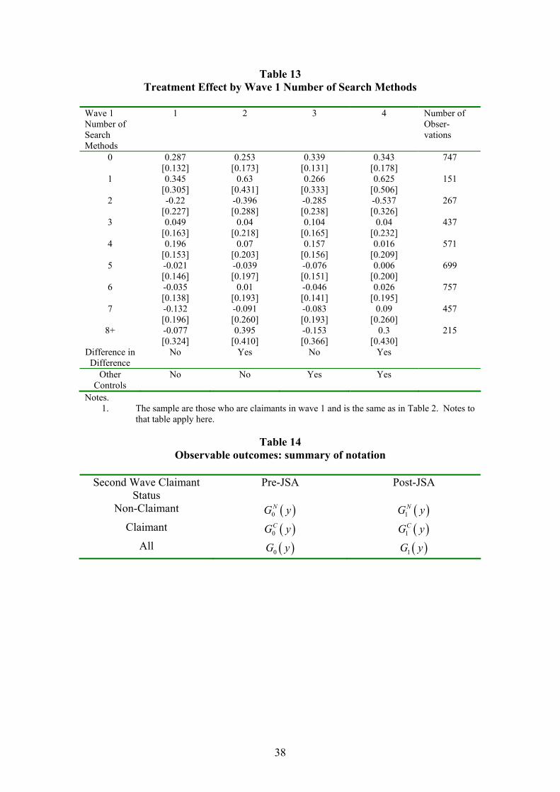
Table 13 Treatment Effect by Wave 1 Number of Search Methods

Wave 1 Number of Search Methods

1 2 3 4 Number of Obser-vations

0.287 0.253 0.339 0.343 747 0 [0.132] [0.173] [0.131] [0.178]

0.345 0.63 0.266 0.625 151 1 [0.305] [0.431] [0.333] [0.506]

-0.22 -0.396 -0.285 -0.537 267 2 [0.227] [0.288] [0.238] [0.326]

0.049 0.04 0.104 0.04 437 3 [0.163] [0.218] [0.165] [0.232] 0.196 0.07 0.157 0.016 571 4

[0.153] [0.203] [0.156] [0.209] -0.021 -0.039 -0.076 0.006 699 5 [0.146] [0.197] [0.151] [0.200] -0.035 0.01 -0.046 0.026 757 6 [0.138] [0.193] [0.141] [0.195] -0.132 -0.091 -0.083 0.09 457 7 [0.196] [0.260] [0.193] [0.260] -0.077 0.395 -0.153 0.3 215 8+ [0.324] [0.410] [0.366] [0.430]

Difference in Difference

No Yes No Yes

Other Controls

No No Yes Yes

Notes. 1. The sample are those who are claimants in wave 1 and is the same as in Table 2. Notes to

that table apply here.

Table 14 Observable outcomes: summary of notation

Second Wave Claimant

Status Pre-JSA Post-JSA

Non-Claimant ( )0NG y ( )1

NG y Claimant ( )0

CG y ( )1CG y

All ( )0G y ( )1G y

39

Table 15

Bounds on Treatment Effects for Movers and Stayers

Proportion Searched in Past Week

Average Number of Search Methods

Lower Bound Upper Bound Lower Bound Upper Bound Bounds From Data Restrictions

Stayers -0.073 (-0.113,-0.037)

0.048 (0.023,0.073)

-0.386 (-0.621,-0.161)

0.566 (0.379,0.746)

Movers -0.382

(-0.529,0.190) 0.618

(0.471,0.810) -4.734

(0.023,0.073) 3.107

(2.330,3.960) Bounds From Intuitive Restrictions

Stayers 0 (0,0)

0.026 (0.001,0.048)

0 (0,0)

0.147 (-0.142,0.316)

Movers -0.195

(-0.339,-0.006) 0.016

(-0.255,0.329) -1.286

(-2.030,-0.453) -0.076

(-1.661,1.747) Notes.

1. The estimates are reported, followed in parentheses by the 95% confidence interval derived from a bootstrap of 1000 replications.

40

Figure 1 The UK Claimant Count. 1984-2004

1000

1500

2000

2500

3000

3500

Cla

iman

t Cou

nt

1985 1990 1995 2000 2005Year

Notes:

1. The source of these data is the administrative records of the welfare system – they can be found at www.nomisweb.co.uk .

2. These are seasonally unadjusted.

Figure 2 Flows On and Off the Claimant Count

150

200

250

300

1988 1993 1998 2003Year

Off-flows('000) On-flows('000)

Notes:

1. The source of these data is the administrative records of the welfare system – they can be found at www.nomisweb.co.uk .

2. These are seasonally adjusted.

41

Figure 3 The Impact of JSA on Outflow Rates From the Claimant Count

-1-.5

0.5

Haz

ard

rate

- diff

eren

ce fr

om A

ugus

t 199

6

1994 1995 1996 1997 1998 1999 2000Year

Notes.

1. These are the monthly dummies for the log hazard rate from the estimation of Cox semi-parametric proportional hazards model for the exit rate from the claimant count. August 1996 is omitted so all hazard rates are relative to that

2. The sample is the inflow between January 1994 and December 2000. 3. The other controls are a quartic in age, gender and regional dummies

Figure 4 Claimant Count and ILO unemployment, 1992-2004

1000

1500

2000

2500

3000

1992 1996 2000 2004Year

Claimant Count ILO Unemployment

Notes:

1. The source of these data is the administrative records of the welfare system for the claimant count and the Labour Force Survey for ILO unemployment – they can be found at www.nomisweb.co.uk .

2. These are seasonally unadjusted.

42

Figure 5 Exits from the Claimant Count: Recorded Destinations

Notes. 1. These data come from the JUVOS administrative database on claimants. 2. The raw data contain more different destinations and these are aggregated measures.

Figure 6

Average Weekly Payment Under UB/IS and JSA

5254

5658

60A

vera

ge W

eekl

y P

aym

ent (

£)

1996 1998 2000 2002Year

Notes. 1. Source is Work and Pensions Statistics, 2002.

.1.2

.3.4

.5.6

prop

ortio

n of

tota

l exi

ts

1995 1996 1997 1998Year

Employment InactivityUnknown

43

Figure 7

The Choice of Search Intensity

Figure 8

The Impact of Stricter Eligibility Conditions

Benefits

bL

bH

sH sL

Benefit rule

s*0 s*1 s*2

Benefits

bL

bH

sH sL Search Intensity

Search Intensity s**

44

Figure 9 The relationship between individual search intensity and Eligibility Conditions

Figure 10

Search Intensity Among Claimants, Part I

Notes. 1. Computations from Labour Force Survey.

.7.75

.8.85

.9Pro

portio

n

1995 1996 1997 1998Year

Looked For Work in Past Month Looked For Work in Past Week

Search Intensity, s

sL

sH

Eligibility Condition, s*

45

Figure 11

Search Intensity Among Claimants, Part II

Notes. 1. Computations from Labour Force Survey.

Figure 12 Average Number of Search Methods Among Claimants

Notes. 1. Computations from Labour Force Survey.

44.2

4.44.6

4.8(m

ean)

nmeth

s

1995 1996 1997 1998Year

.02.04

.06.08

.1.12

Propo

rtion

1995 1996 1997 1998Year

Want Job - No Search Don't Want a Job

46

Figure 13 The Average Number of Search Methods Among the Non-employed, 1995-1998

.3.3

5.4

.45

.5A

vera

ge N

umbe

r of S

earc

h M

etho

ds

1995 1996 1997 1998Year

Notes. 1. Computations from Labour Force Survey.

47

Appendix A: A Typical Jobseeker’s Agreement

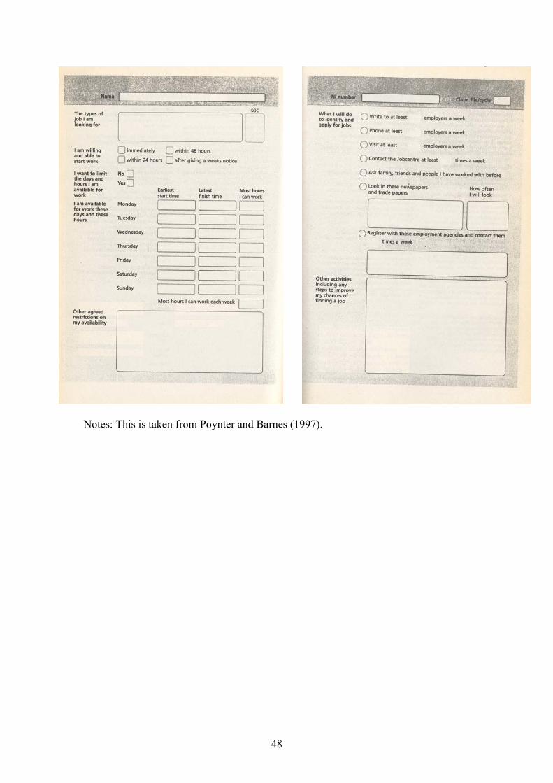
48

Notes: This is taken from Poynter and Barnes (1997).

49

Appendix B

A Simple Model of the Determination of Search Intensity The value function for being without a job can be written as:

( ),max ( ) ( ) ( )u us r u ur

V b s V w V dF w c sβ λ = + − − ∫ (10)

where r is the reservation wage, s is search intensity, F(w) is the distribution function of wage offers, β is the discount factor, ( )u sλ is the arrival rate of offers and ( )uc s is the cost of search effort. Before analysing the behaviour of someone without a job it is useful to discuss the behaviour of someone with a job. Similarly, the value function for an employed worker at wage w can be written as:

( ) ( ) ( ) ( ) ( )max ( ) ( ) uw e ew

V w w s V x V w dF x V V w c sβ λ δ = + − + − − ∫ (11)

where δ is the rate of job loss, assumed to be exogenous. This can be thought of as leading to a solution for search intensity, s(w). Differentiating (11) we have that:

( ) ( )( ) ( )( )1'

1e

V ws w F wβ δ λ

=+ + −

(12)

and, integrating by parts, one then has:

( ) ( )( ) ( )( )( ) ( )( )

1( ) ( ) 1 '( )

( ) 1w w we

F xV x V w dF x F x V x dx dx

s x F xβ δ λ−

− = − = + + −∫ ∫ ∫ (13)

Substituting this into (11), the first-order condition for the choice of search intensity by a worker employed at wage w can be written as:

( )( ) ( )( )

( ) ( )( ) ( )( )1'

( ) 1e

ewe

s w F xdx c s w

s s x F xλ

β δ λ∂ −

=∂ + + −∫ (14)

Note that the solution to this is independent of the level of benefits paid when unemployed. Now consider the behaviour of those without a job. Using (13) one can write the value function for the unemployed as:

( ) ( )( )( ) ( )( ),

1max ( )

( ) 1u

s r u ure

F x dxV b s c s

s x F xβ λ

β δ λ−

= + −+ + −∫ (15)

The reservation wage will be the level of the wage such that ( ) uV r V= . For given levels of benefit and search intensity this will solve the equation:

( ) ( ) ( )( )( ) ( )( )

1( ) ( ) ( ( ))

( ) 1u e u ere

F x dxr b s s r c s c s r

s x F xλ λ

β δ λ−

= + − − + + + −∫ (16)

One can think of a solution to this equation ( ),r b s where the reservation wage depends positively on b as differentiation of (16) leads to: :

( ) ( )( )( ) ( )( )( ) 1

01

e

u

s x F xrb s F x

β δ λβ δ λ+ + −∂

= >∂ + + −

(17)

The dependence of r on s is ambiguous in sign as differentiation of (16) leads to:

50

( ) ( )( )( ) ( )( )

( ) ( )( )( ) ( )( ) ( )

( ) 1 1'

1 ( ) 1e u

uru e

s x F x F x dxsr c ss ss F x s x F x

β δ λ λβ δ λ β δ λ

+ + − −∂∂= −

∂ ∂+ + − + + − ∫ (18)

The intuition is that an increase in search intensity makes the individual more (resp. less) choosy if the marginal return to search activity is positive (resp negative). Using these results on b, let us know differentiate (15) to work out the impact of the value of being unemployed of b and s: We have:

( ) ( )( ) 0

1

u

u

Vb s F x

β δββ δ λ

∂ += >

∂ + + − (19)

and:

( ) ( )( )( ) ( )( )

( ) ( )( ) ( )1

'1 ( ) 1

uu

uru e

F x dxsV c ss ss F x s x F x

λβ δββ δ λ β δ λ

−∂∂ += −

∂ ∂+ + − + + − ∫

which is first increasing and then decreasing in s. Also of importance is the dependence of the optimal b on s. This is negative as a rise in b raises the reservation wage and this reduces the return to searching. Hence the indifference curves must look as drawn in Figure 7.

51

Appendix C Descriptive Statistics and Analysis of Treatment and Control Groups

Table C1

Descriptive Statistics

All control Treatment Mean s.d. Mean s.d. Mean s.d.

Wave 1 Search Activity

Don't Want Job 0.065 0.247 0.066 0.248 0.065 0.246 Want Job but

no Search 0.093 0.291 0.090 0.286 0.096 0.295

Searched in last 4 weeks but not

last week

0.052 0.222 0.050 0.217 0.054 0.227

Number of search methods

4.22 2.47 4.24 2.48 4.19 2.46

Wave 2 Search Activity and Claimant Status Non-claimant

Non-employed 0.16 0.37 0.13 0.33 0.19 0.40

Claimant 0.65 0.48 0.70 0.46 0.60 0.49 Don't Want Job 0.07 0.26 0.07 0.26 0.08 0.27 Want Job but

no Search 0.10 0.29 0.10 0.30 0.09 0.29

Searched in last 4 weeks but not

last week

0.04 0.21 0.05 0.21 0.04 0.20

Searched in Past Week

0.60 0.49 0.61 0.49 0.59 0.49

Employed 0.19 0.39 0.17 0.38 0.20 0.40 Number of

search methods 3.43 2.81 3.48 2.80 3.38 2.82

Personal Characteristics Male 0.72 0.45 0.73 0.44 0.72 0.45 Black 0.04 0.19 0.04 0.19 0.04 0.20 Asian 0.04 0.20 0.04 0.20 0.04 0.20

Experience 18.50 12.58 18.67 12.53 18.33 12.64 University Graduate

0.13 0.33 0.11 0.32 0.14 0.35

`A' Level or equivalent

0.21 0.41 0.21 0.41 0.21 0.40

No qualifications

0.37 0.48 0.39 0.49 0.35 0.48

Ever worked 0.92 0.26 0.93 0.25 0.92 0.28 Duration since

last job 3.11 4.36 3.10 4.35 3.13 4.37

Married 0.62 0.49 0.63 0.48 0.61 0.49 Number of

children 0.76 1.19 0.77 1.20 0.74 1.18

Age of youngest child

2.31 4.39 2.33 4.39 2.29 4.40

tyne & wear 0.02 0.15 0.03 0.16 0.02 0.15 Rest of north 0.04 0.19 0.04 0.19 0.04 0.19

South yorkshire 0.03 0.16 0.02 0.15 0.03 0.16 West yorkshire 0.04 0.19 0.03 0.18 0.04 0.19 rest of yorks+ Humberside

0.02 0.15 0.03 0.16 0.02 0.14

East midlands 0.07 0.25 0.07 0.25 0.06 0.25

52

east anglia 0.03 0.17 0.02 0.16 0.03 0.17 inner london 0.08 0.26 0.08 0.27 0.07 0.26 outer london 0.08 0.27 0.07 0.26 0.08 0.27 South west 0.07 0.25 0.06 0.24 0.07 0.26

West midlands (met)

0.06 0.24 0.06 0.25 0.06 0.24

rest of west midlands

0.04 0.18 0.04 0.18 0.04 0.18

Greater manchester

0.04 0.20 0.04 0.21 0.04 0.20

Merseyside 0.03 0.18 0.03 0.18 0.03 0.18 rest of north-

west 0.03 0.17 0.03 0.17 0.03 0.17

Wales 0.05 0.22 0.05 0.22 0.05 0.22 Strathclyde 0.05 0.22 0.05 0.22 0.05 0.21

rest of scotland 0.05 0.21 0.04 0.20 0.05 0.21 Northern ireland

0.06 0.23 0.06 0.24 0.05 0.23

Notes. 1. All this data refers to those who are claimants and to 1996 only.

53

Table C2

The Balancing of Treatment and Control Groups

1 2 3 4 Sample All All Non-

employed Non-employed

Don’t Want Job -0.012 -0.034 -0.024 -0.041 [0.034] [0.036] [0.036] [0.038] Want Job but no Search -0.015 -0.021 -0.032 -0.034 [0.031] [0.032] [0.033] [0.035] Searched in last 4 weeks but not last week

0.017 0.016 0.027 0.025

[0.032] [0.032] [0.035] [0.036] Number of search methods

-0.004 -0.007 -0.006 -0.008

[0.004] [0.004] [0.005] [0.005] Male -0.022 -0.011 [0.028] [0.032] Black 0.039 0.022 [0.038] [0.040] Asian -0.012 -0.008 [0.036] [0.039] Experience -0.002 0 [0.002] [0.003] Experience squared 0 0 [0.000] [0.000] University Graduate 0.048 -0.018 [0.024]* [0.028] `A’ Level of equivalent 0.007 0.017 [0.021] [0.023] No qualifications -0.032 -0.031 [0.018] [0.020] ever had paid job -0.057 -0.073 [0.030] [0.034]* Duration since last job 0.009 0.009 [0.004]* [0.004]* Duration squared 0 0 [0.000] [0.000] Married 0.005 0.009 [0.028] [0.032] Number of children -0.009 0 [0.016] [0.017] Age of youngest child -0.001 -0.004 [0.004] [0.004] Married* Male 0.009 0.009 [0.033] [0.037] No. of Kids * Male 0.006 -0.002 [0.018] [0.019] Age of youngest child* Male

0.001 0.003

[0.004] [0.005] tyne & wear 0.009 0.032 [0.049] [0.055] rest of northern region -0.008 0.001

54

[0.039] [0.044] south Yorkshire 0.034 0.048 [0.048] [0.052] west Yorkshire 0.003 0.014 [0.042] [0.046] rest of yorks & Humberside -0.088 -0.05 [0.048] [0.055] east midlands -0.025 -0.001 [0.034] [0.038] east anglia 0.06 0.082 [0.044] [0.050] inner London -0.068 -0.048 [0.033]* [0.036] outer London 0.024 0.062 [0.032] [0.035] south west 0.022 0.018 [0.033] [0.038] west midlands (met county) -0.024 -0.009 [0.035] [0.039] rest of west midlands -0.026 -0.01 [0.042] [0.046] Greater Manchester -0.018 0 [0.039] [0.043] Merseyside -0.019 0.016 [0.043] [0.048] rest of north west -0.04 -0.041 [0.044] [0.052] Wales 0.002 0.034 [0.036] [0.040] Strathclyde -0.017 0.023 [0.037] [0.041] rest of Scotland 0.018 0.021 [0.037] [0.042] northern Ireland -0.039 -0.035 [0.036] [0.040] Observations 5292 5207 4301 4227 p-value 0.82 0.22 0.57 0.64

Notes. 1. These tables report the marginal effects from a probit model in which the dependent

variable is one if the observation comes from the treatment group and zero if it comes from the control group. Standard errors in brackets and * denotes coefficient significant at 5%; ** significant at 1%.

2. The reported p-value is from a test of the hypothesis that all the slope coefficients are zero – this is a test that the treatment and control groups are ‘balanced’.

3. The first two columns report the estimates when the sample is all who are claimants at wave 1 and the second two columns when the sample is restricted to those who had not exited to employment at wave 2.

55

Appendix D Identifying Treatment Effects by Final Claimant Status

With the imposition of the identifying assumptions described in the text we must have the following relationships between the observed distribution functions and the ones we would like to observe: 0 0

N NNG F= (20)

0 11 11

NN NN CN CNNN NN CN CNN

NN CN NN CN

p F p Fp F p FGp p p p

++= =

+ + (21)

0 00

CC CC CN CNC

CC CN

p F p FGp p

+=

+ (22)

1 1C CCG F= (23)

From the discussion in the text, we know that ( ), ,CN NN CCp p p are identified. The lack of identification on the 'F s can be seen from the fact that there are four equations and five unknowns. (20) says that 0

NNF can be identified and (23) that 1CCF

can be identified. Then, using (20) and (21) we have that:

( ) 1 0

1

NN CN N NN NCN

CN

p p G p GF

p+ −

= (24)

This implies that the identification problem relates to 0CCF and 0

CNF . So what can be identified? Denote the overall distribution of y under the pre-JSA regime as ( )0G y

and under the post-JSA regime as ( )1G y . We must have the following:

( )1 1 1NN CN N CC CG p p G p G= + + (25)

( )0 0 0NN N CC CN CG p G p p G= + + (26)

Taking differences and then using the relationships in (20) to (23) we end up with: CN CN CC CCG p F p F∆ = ∆ + ∆ (27) so that:

CN CN CC CC

CN CC CN CC

p F p F Gp p p p

∆ + ∆ ∆=

+ + (28)

i.e. the change in the distribution function of outcomes between the treatment and control divided by the fraction of the population to have a non-zero treatment effect can be interpreted as the average treatment effect across those who remain in claimant status post-JSA and those who are moved out of claimant status. This is a fairly obvious result as these are the only groups with a non-zero treatment effect. And the overall treatment effect can be obtained by comparing the distribution outcomes between treatment and control groups.

56

References Abbring, Jaap H., Gerard J. van den Berg and Jan van Ours (1997) “The effect of unemployment insurance sanctions on the transition rate from unemployment to employment”, Working Paper, Tinbergen Institute, Amsterdam. Angrist, Joshua D and Guido W Imbens (1994) “Identification and Estimation of Local Average Treatment Effects”, Econometrica, 62: 467-75. Ashenfelter, Orley, David Ashmore, and Olivier Deschênes, (1998). "Do Unemployment Insurance Recipients Actively Seek Work? Evidence From Randomized Trials in Four U.S. States," Princeton IR Section Working Paper, No. 412. Barron, John M. and Wesley Mellow (1979) “Search Effort in the Labor Market”, Journal of Human Resources, 14, 390-404. Ben-Horim, Moshe and Dror Zuckerman, 1987, “The Effect of Unemployment Insurance on Unemployment Duration”, Journal of Labor Economics, 5(3), July, pages 386-90. Van den Berg, Gerard J., (1990), “Search Behaviour, Transitions to Nonparticipation and the Duration of Unemployment”, Economic Journal; 100(402), September, pages 842-65. van den Berg, Gerard J & Bas van der Klaauw, (2001), "Counselling and Monitoring of Unemployed Workers: Theory and Evidence from a Controlled Social Experiment," CEPR Discussion Papers 2986, C.E.P.R. Discussion Papers van den Berg, Gerard J.; Bas van der Klaauw, and Jan van Ours, (2004) ”Punitive Sanctions and the Transition Rate from Welfare to Work”, Journal of Labor Economics, 22, 211-41. Black, Dan A., Jeffrey A. Smith, Mark C. Berger and Brett J. Noel (2003) “Is the Threat of Reemployment Services More Effective Than the Services Themselves? Evidence from Random Assignment in the UI System”, American Economic Review, 93, 1313-1327. Blank, R. and Card, D., (1992), `Recent Trends in Insured and Uninsured Unemployment: Is There an Explanation ?', Quarterly Journal of Economics, vol. 61, No. 4, pp 1157-90. Blau, David M. and Philip, K. Robins, 1990, “Job Search Outcomes for the Employed and Unemployed”, Journal of Political Economy; 98(3), June, pages 637-55. Blundell, Richard, John Ham, and Costas Meghir, 1987, “Unemployment and Female Labour Supply”, Economic Journal; 97, Supplement, pages 44-64.

57

Blundell, Richard, John Ham, and Costas Meghir, 1998, “Unemployment, Discouraged Workers and Female Labour Supply”, Research in Economics, 52, 103-131. Boone, Jan and Jan van Ours (2000) “Modeling Financial Incentives to Get Unemployed Back to Work”, IZA Discussion Paper, No. 108. Boone, Jan, Peter Fredriksson, Bertil Holmlund and Jan van Ours (2001) “Optimal Unemployment Insurance with Monitoring and Sanctions”, IZA Discussion Paper, No. 401. Burdett, Kenneth, Nicholas M. Kiefer, Dale T. Mortensen, and George Neumann, 1984, “Earnings, Unemployment, and the Allocation of Time over Time”, Review of Economic Studies; 51(4), October, pages 559-78. Burdett, Kenneth, and Dale T. Mortensen, 1978, “Labor Supply Under Uncertainty” in: Ronald G. Ehrenberg (ed) Research in Labor Economics, Greenwich Ct: JAI Press. Crepon, Bruno, Muriel Dejemeppe and Marc Gurgand (2004) “Counseling the unemployed: does it lower unemployment duration and recurrence?”, unpublished CREST. Decker, Paul T., Robert B. Olsen, Lance Freeman and Daniel Klepinger (2000) “Assisting Unemployment Insurance Claimants: The Long-Term Impacts of the Job Search Assistance Demonstration”, Dolton, Peter & O'Neill, Donal, (1995). "The Impact of Restart on Reservation Wages and Long-Term Unemployment," Oxford Bulletin of Economics and Statistics, 57, 451-70. Dolton, Peter & O'Neill, Donal, (1996). "Unemployment Duration and the Restart Effect: Some Experimental Evidence," Economic Journal, 106, 387-400. Dolton, Peter and Donal O’Neill (2002) “The Long-Run Effects of Unemployment Monitoring and Work-Search Programs: Experimental Evidence from the United Kingdom”, Journal of Labor Economics, 20, 381-403. Flinn, Christopher J. and James J. Heckman, 1983, “Are Unemployment and Out of the Labor Force Behaviorally Distinct Labor Force States?” Journal of Labor Economics; 1(1), January, pages 28-42. Gregg, P. and Wadsworth, J., (1996), ‘How Effective are State Employment Agencies?’, Oxford Bulletin of Economics and Statistics, Vo. 58, August, pp. 443-468. Grubb, David (2000) “Eligibility Criteria for Unemployment Benefits”, OECD Economic Studies, 31, 147-183.

58

Hamermesh, Daniel S., (1982) “The Interaction between Research and Policy: The Case of Unemployment Insurance”, American Economic Review; 72(2), May, pages 237-41. Jones, Stephen R.G. and W. Craig Riddell, 1999, “The Measurement of Unemployment: An Empirical Approach”, Econometrica; 67(1), January , pages 147-61. Klepinger, Daniel H., Terry R. Johnson, Jutta M. Joesch and Jacob M. Benus (1997) “Evaluation of the Maryland Unemployment Insurance Work Search Demonstration”, http://workforcesecurity.doleta.gov/dmstree/op/op98/op_02-98.pdf . Machin, Stephen and Olivier Marie (2004) “Crime and Benefit Sanctions”, CEP LSE Discussion Paper No. 645, August 2004, http://cep.lse.ac.uk/pubs/download/dp0645.pdf McKay, Stephen, Alison Smith, Rachel Youngs and Robert Walker (1999) “Unemployment and Jobseeking after the introduction of Jobseeker’s Allowance”, Department of Social Security, Research Report No. 99. Meyer, Bruce D., 1995, “Lessons from the U.S. Unemployment Insurance Experiments” Journal of Economic Literature; 33(1), March, pages 91-131. Mortensen, Dale T., 1986, “Job Search and Labor Market Analysis” in Ashenfelter, Orley and Richard Layard (eds.) Handbook of labor economics, Volume 2, Amsterdam: North-Holland, pages 849-919. Poynter, Richard and Martin Barnes (1997) Jobseeker’s Allowance Handbook, London: Child Poverty Action Group. Rayner, Elizabeth, Sohagini Shah, Richard White, Len Dawes and Kevin Tinsley (2000) “Evaluating Jobseeker’s Allowance: A Summary of the Research Findings”, Department of Social Security, Research Report No. 116. Schmitt, J. and Wadsworth, J. (1993), `Unemployment Benefit Levels and Search Activity,' Oxford Bulletin of Economics and Statistics, Vol. 55, No. 1, pp 1-20. Schmitt, John and Jonathan Wadsworth (2002) “You Won’t Feel the Benefit: A Pseudo-Panel Analysis of Changing Unemployment Benefit Entitlement and Unemployment Outflows in Britain”, Centre for Economic Performance, LSE. Smith, Alison, Rachel Youngs, Karl Ashworth, Stephen McKay and Robert Walker with Peter Elias and Abigail McKnight (2000) “Understanding the Impact of Jobseeker’s Allowance”, Department of Social Security, Research Report No. 111. Sweeney, Kate and Denis McMahon (1998) “The effect of Jobseeker’s Allowance on the claimant count”, Labour Market Trends, 106, 195-203.

59

Trickey, Heather, Karen Kellard, Robert Walker, Karl Ashworth and Alison Smith (1998) “Unemployment and Jobseeking: Two Years On”, Department of Social Security, Research Report No. 87. Wadsworth, J. (1991), `Unemployment Benefits and Search Effort in the U.K. Labour Market,' Economica, vol. 58, pp. 17-34.