you for downloading this document from the rmit research...

Thank

Citatio

See th

Version

Copyri

Link to

you for do

on:

is record i

n:

ght Statem

o Published

wnloading

in the RMI

ment: ©

d Version:

this docum

IT Researc

ment from

ch Reposit

the RMIT R

ory at:

Research RRepository

PLEASE DO NOT REMOVE THIS PAGE

Vu, L and Baulch, B 2011, 'Assessing alternative poverty proxy methods in rural Vietnam',Oxford Development Studies, vol. 39, no. 3, pp. 341-362.

http://researchbank.rmit.edu.au/view/rmit:17730

Submitted Version

2011 Oxford Department of International Development

http://dx.doi.org/10.1080/13600818.2011.599207

http://researchbank.rmit.edu.au/

For Peer Review O

nly

Assessing Alternative Poverty Proxy Methods in Vietnam

Journal: Oxford Development Studies

Manuscript ID: CODS-2010-0036.R1

Manuscript Type: Original Article

Keywords: poverty, rural sector, Vietnam

URL: http:/mc.manuscriptcentral.com/cods Email: [email protected]

Oxford Development Studies

For Peer Review O

nly

1

ASSESSING ALTERNATIVE POVERTY PROXY METHODS IN RURAL VIETNAM

20 December 2010

Abstract

This paper compares and contrasts the use of four ‘short-cut’ methods for identifying poor households: (i) the poverty probability method; (ii) OLS regressions; (iii) principal components analysis; and, (iv) quantile regressions. After evaluating these four methods using two alternative criteria (total and balanced poverty accuracy) and representative household survey data from rural Vietnam, we conclude that the poverty probability method─which can correctly identify around four-fifths of poor and non-poor households─ is the most accurate ‘short-cut’ method for measuring poverty for specific sub-populations, or in years when household surveys are not available. We then test the performance of the poverty probability method with different poverty lines and using an alternative household survey, and find it to be robust.

Page 2 of 37



123456789101112131415161718192021222324252627282930313233343536373839404142434445464748495051525354555657585960

For Peer Review O

nly

2

I. Introduction

In most developing countries, it is only feasible to conduct detailed household surveys every few using relatively small samples of households. The results of these surveys can usually only be disaggregated to the regional or provincial level, and cannot be disaggregated for many population groups that are of interest to policy makers (for example, specific occupations or ethnic groupings). However, government and donor agencies often require that poverty should be monitored on an annual basis for specific administrative or project areas, or require projects demonstrate their impact on specific groups or occupations. Poverty measurement using household surveys is also difficult, expensive and time consuming, requiring detailed information is collected on all the different components of household expenditures and/or incomes.

Short-cut methods for measuring monetary poverty in specific areas or sub-populations have therefore been devised for around 30 developing countries, most noticeable by the Grameen Foundation and USAID Poverty Assessment Tools project.1 Typically these methods use 10 to 20 easily verifiable indicators to obtain an index or score that is highly correlated with household poverty status. Using these short-cut methods, non-specialists can collect data for each household in the field in ten to fifteen minutes which, when combined with the coefficients from models estimated with nationally representative household survey data,can provide a reasonably accurate prediction of household’s poverty status. However, there have been few attempts to systematically compare such methods (especially using out-of-sample predictions).

This paper compares and contrasts the use of four ‘short-cut’ methods for measuring monetary poverty in rural Vietnam. These three methods, which we shall hereafter describe collectively as poverty proxy methods, are: (i) the poverty probability method; (ii) OLS regressions; (iii) principal components analysis and (iv) quantile regression. Each of these poverty proxy methods have been used in the past in Vietnam using different datasets and poverty lines (see Section II), but to date there has been no study which compares the accuracy of these different methods using the same data set, and few which have compare their out-of-sample predictive power using different data sets. Accordingly, this study uses the 2006 Vietnamese Household Living Standards Survey (VHLSS 2006) to test these four methods for rural households using a common international poverty line ($1.25/day in 2005 PPP terms). After evaluating these four methods using two alternative criteria (total and balanced poverty accuracy, which are explained below), we also test the models’ performance with different poverty lines and its out-of-sample performance using an alternative household survey (the VHLSS of 2004). We conclude that the poverty probability method is the most accurate ‘short-cut’ method for measuring poverty for specific sub-populations of interest, or in years when representative household surveys are not available.

II. Literature Review

This section provides a brief overview of six previous applications of poverty proxy methods in Vietnam in approximate chronological order.2 While two of these studies have been developed independently by Vietnam-based researchers, the remaining four are part of larger cross-country efforts to development ‘short-cut’ poverty assessment for various development organisations.

1 See www.microfinance.org/#Poverty_Scoring and www.povertytools.org 2 This section draws on Chen and Schreiner (2009).

Page 3 of 37



123456789101112131415161718192021222324252627282930313233343536373839404142434445464748495051525354555657585960

For Peer Review O

nly

3

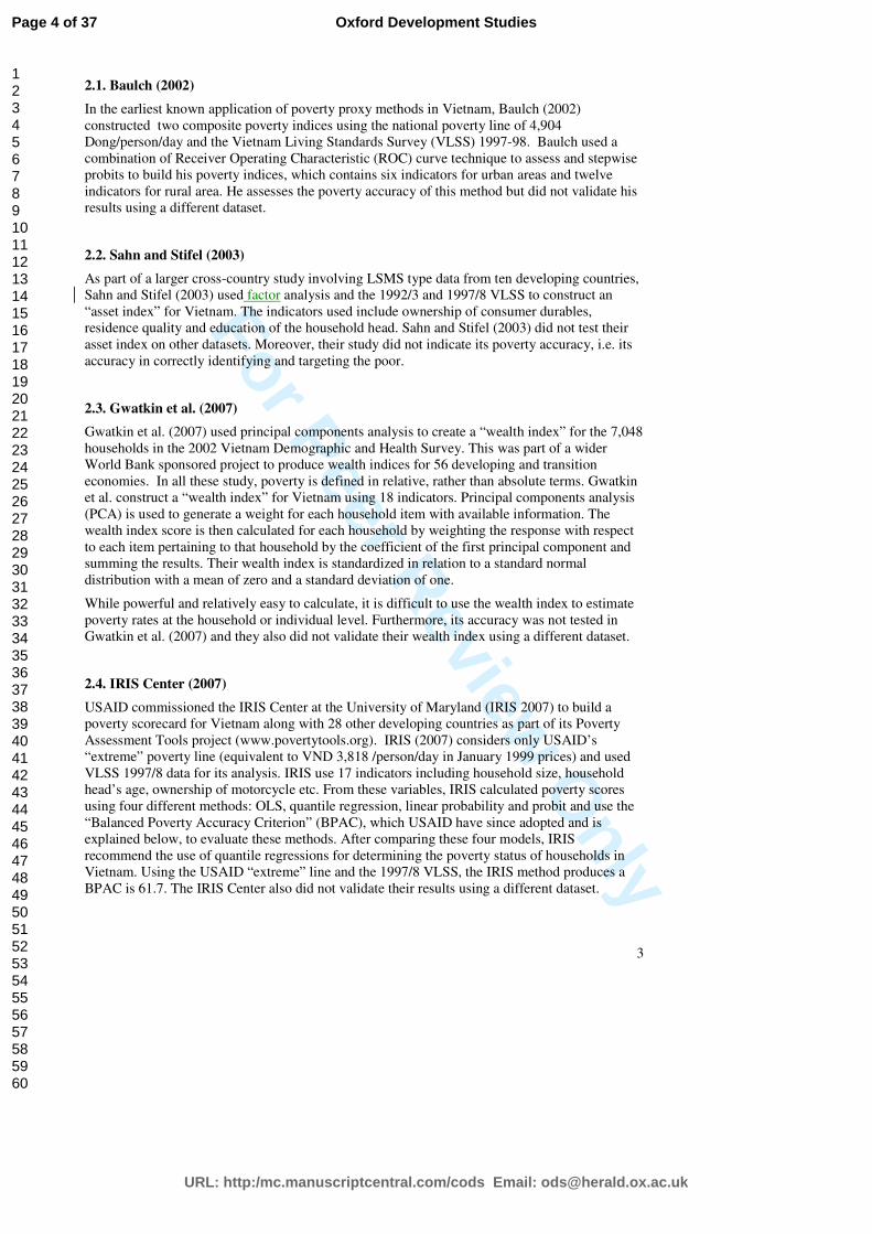
2.1. Baulch (2002)

In the earliest known application of poverty proxy methods in Vietnam, Baulch (2002) constructed two composite poverty indices using the national poverty line of 4,904 Dong/person/day and the Vietnam Living Standards Survey (VLSS) 1997-98. Baulch used a combination of Receiver Operating Characteristic (ROC) curve technique to assess and stepwise probits to build his poverty indices, which contains six indicators for urban areas and twelve indicators for rural area. He assesses the poverty accuracy of this method but did not validate his results using a different dataset.

2.2. Sahn and Stifel (2003)

As part of a larger cross-country study involving LSMS type data from ten developing countries, Sahn and Stifel (2003) used factor analysis and the 1992/3 and 1997/8 VLSS to construct an “asset index” for Vietnam. The indicators used include ownership of consumer durables, residence quality and education of the household head. Sahn and Stifel (2003) did not test their asset index on other datasets. Moreover, their study did not indicate its poverty accuracy, i.e. its accuracy in correctly identifying and targeting the poor.

2.3. Gwatkin et al. (2007)

Gwatkin et al. (2007) used principal components analysis to create a “wealth index” for the 7,048 households in the 2002 Vietnam Demographic and Health Survey. This was part of a wider World Bank sponsored project to produce wealth indices for 56 developing and transition economies. In all these study, poverty is defined in relative, rather than absolute terms. Gwatkin et al. construct a “wealth index” for Vietnam using 18 indicators. Principal components analysis (PCA) is used to generate a weight for each household item with available information. The wealth index score is then calculated for each household by weighting the response with respect to each item pertaining to that household by the coefficient of the first principal component and summing the results. Their wealth index is standardized in relation to a standard normal distribution with a mean of zero and a standard deviation of one.

While powerful and relatively easy to calculate, it is difficult to use the wealth index to estimate poverty rates at the household or individual level. Furthermore, its accuracy was not tested in Gwatkin et al. (2007) and they also did not validate their wealth index using a different dataset.

2.4. IRIS Center (2007)

USAID commissioned the IRIS Center at the University of Maryland (IRIS 2007) to build a poverty scorecard for Vietnam along with 28 other developing countries as part of its Poverty Assessment Tools project (www.povertytools.org). IRIS (2007) considers only USAID’s “extreme” poverty line (equivalent to VND 3,818 /person/day in January 1999 prices) and used VLSS 1997/8 data for its analysis. IRIS use 17 indicators including household size, household head’s age, ownership of motorcycle etc. From these variables, IRIS calculated poverty scores using four different methods: OLS, quantile regression, linear probability and probit and use the “Balanced Poverty Accuracy Criterion” (BPAC), which USAID have since adopted and is explained below, to evaluate these methods. After comparing these four models, IRIS recommend the use of quantile regressions for determining the poverty status of households in Vietnam. Using the USAID “extreme” line and the 1997/8 VLSS, the IRIS method produces a BPAC is 61.7. The IRIS Center also did not validate their results using a different dataset.

Page 4 of 37



123456789101112131415161718192021222324252627282930313233343536373839404142434445464748495051525354555657585960

For Peer Review O

nly

4

2.5. Linh Nguyen (2007)

In a paper for the Asian Development Bank, Linh Nguyen (2007) uses multiple regression techniques to assess poverty using the VHLSS 2002 data. This technique detects variables or predictors that are correlated with a household’s consumption expenditure and consequently, its poverty status. She used bivariate and multivariate analysis to narrow down the number of variables from an initial list of 60 variables to 22 indicators in rural and 15 indicators in urban areas. Linh Nguyen (2007) validated her results using the VLSS 1998 data and a subset of the VHLSS 2002 (for Thanh Hoa and Nghe An provinces).

2.6 Chen and Schreiner (2009)

Schreiner and colleagues have developed poverty scorecards for the Grameen Foundation in 28 developing countries (www.microfinance.com/#Poverty_Scoring). Chen and Schreiner (2009) develop a simple poverty “scorecard” for Vietnam with 10 indicators selected from an initial list of 150 indicators drawn from the VHLSS 2006. Each indicator is first screened with an entropy-based “uncertainty coefficient” that measures how well each indicator predicts poverty on its own. Their final indicator selection uses both judgement and statistics (a forward stepwise logit). The final scorecard is built using a PPP $1.75/day poverty line and a logit regression.3 One advantage of Chen and Schreiner (2009) method is their validation of the scorecard using the VHLSS 2004. However, its performance is not compared to those of other methods.

Appendix A1 summarises and compares the different indicators that were used to predict poverty in each of these studies, and compares them with those proposed in this paper.

It should be noted that four of the six of these poverty proxy methods have an explicit focus on monetary poverty (identified according to whether a household’s per capita expenditure is above or below a pre-determined absolute poverty line) while the other two methods concern asset poverty. None of the methods consider the wider non-monetary dimensions of poverty that are considered in, for example, the UNDP’s Multidimensional Poverty Index (Alkire and Santos, 2010). While focusing on monetary poverty is obviously restrictive, it does reflect the principal way in which poverty is measured in Vietnam (and many other countries).

III. Data and Methods

We used data from the VHLSS 2006, the most recent available national income and expenditure survey in Vietnam. The data cover over 45,000 households in rural and urban areas. It includes information on household income, assets, expenditure4 and other socio-economic dimensions. Using the VHLSS06 data, we compare the results of four poverty proxy approaches. In addition, we used the VHLSS 2004 and the Thanh Hoa Resurvey data for validation of estimates of poverty rates.

There are two “official” poverty lines in Vietnam. The General Statistical Office (GSO) defines a food poverty line based on the expenditure required to obtain 2100 calories per person per day. Based on the food poverty line, the national poverty lines are then defined as the food poverty lines plus non-food expenditure by a reference group with food expenditure close to the food poverty line. The GSO’s poverty line is equivalent to VND 7,011/person/day at January, 2006 prices. The GSO’s poverty line is, however, based on a food basket which was first estimated in

3 Chen and Schreiner justify the use of a PPP $ 1.75/day poverty line by saying that it is close to the national poverty line. 4 The expenditure data are collected from a subsample of just over 9,000 households.

Page 5 of 37



123456789101112131415161718192021222324252627282930313233343536373839404142434445464748495051525354555657585960

http://www.microfinance.com/#Poverty_Scoring

For Peer Review O

nly

5

1993, and has only been updated by inflating its food and on-food components by the relevant price indices.

An alternate set of poverty lines are set by Ministry of Labour, Invalids, and Social Affairs (MOLISA) for 2006–2010 as VND 6,575/person/day for rural areas and VND 8,548/person/day for urban areas (Chen and Schreiner 2009). The MOLISA poverty lines are administratively determined and updated periodically to reflect changes in both the cost of living and living standards. In contrast to the General Statistics Office, MOLISA’s poverty lines are based on per capita incomes. At the present time, there is an ongoing debate about the updating of the MOLISA poverty lines for the 2011 to 2015 period.

Because of the dated nature of both of the GSO and MOLISA poverty lines, the poverty lines used in our analysis are the international poverty lines of PPP $1.25 and $2.00 per person per day. These lines were calculated by the World Bank using household survey data from 116 countries together with the results of the 2005 International Comparisons Project (Ravallion et al., 2008). In Vietnamese Dong, the $1.25/day line is equivalent to VND 242,250/person/month while the $2/day line is VND 387,600/person/month, in January, 2006 prices. These are the poverty lines which most international and bilateral donors use for monitoring the MDGs. Those with incomes (or expenditures) of less than PPP $1.25/day are usually regarded as extremely poor, while those living between PPP $1.25 and $2/day as moderately poor.

We use two criteria to assess the accuracy in predicting poverty. The first criterion is total accuracy, i.e. weighted average of poverty accuracy and non-poverty accuracy. It is calculated by the following formula:

Total accuracy= Headcount index × Poverty accuracy+ (1- Headcount index) × Non-poor accuracy. (1)

Thus total accuracy, which will always vary between 0 and 100, shows the percentage of people correctly identified as poor and non-poor.

The second criterion is BPAC index, adopted by USDA in its poverty assessment. The BPAC index is calculated by the following formula

BPAC= (Inclusion – |Under-coverage – Leakage|) x [100 ÷ (Inclusion + Under-coverage)] (2)

in which, Under-coverage= the “true” poor incorrectly predicted as non-poor, expressed as a percentage of total “true” poor; Leakage = “true” non-poor incorrectly predicted as poor, expressed as a percentage of total “true” poor; Inclusion= the “true” poor correctly predicted as poor, expressed as a percentage of total “true” poor. In other words, BPAC is the poverty accuracy minus the difference between under-coverage and leakage expressed as percentages of total “true” poor. Note that unlike, Total Accuracy, BPAC can take negative values when the absolute difference between under-coverage and leakage exceeds poverty accuracy.

In line with Prosperity Initiative’s goal of reducing poverty at scale (that is having systemic impacts on poverty reduction that extend beyond the communities in which the organisation is working) our preferred criterion is the BPAC. As Total Accuracy combines accurate identification of both poor and non-poor, this measure is only useful if one is interested in an aggregate assessment of poverty status without wanting to target the poor specifically. Indeed, in some cases, a proxy method with high Total Accuracy can give a highly inaccurate identification of poor people. For example in Table 5, at the cut-off point of 0.5, Total Accuracy is the highest (82.74) but only 38.1 percent of the poor are correctly identified. So for this reason, we focus on the BPAC in assessing different poverty proxy models.

We also employ Receiving Operating Characteristic (ROC) curves to show the accuracy of different poverty proxy methods. ROC curves are diagrams which portray the ability of different Deleted: non-parametric

Page 6 of 37



123456789101112131415161718192021222324252627282930313233343536373839404142434445464748495051525354555657585960

For Peer Review O

nly

6

diagnostics tests to distinguish between a binary outcome, and were originally developed for use in electrical engineering and signal processing (Baulch, 2002; Wodon, 1997). A ROC curve shows the ability of a test to distinguish between two states or conditions. In poverty analysis, ROC curves plot the probability of a test correctly identifying a poor person as poor (which is called the test’s “sensitivity”) on the vertical axis against one minus the probability of the same test correctly classifying a non-poor person as non-poor on the horizontal axis (which is called the test’s “specificity”). Typically, ROC curves are concave and embody a trade-off between coverage of the poor and inclusion of the non-poor (see Figures 1 to 3 below). As long as an indicator or index increases in value as the likelihood of poverty increases, then the area under an ROC curve—which will always vary between zero and one—can be used for ranking their relative efficacy as poverty proxies. An ROC curve with an area of 0.5 will lie mostly below the leading diagonal.

IV. Constructing poverty proxies for rural Vietnam

1. Poverty indicators

In order to assess poverty, we use three alternative poverty proxy methods: the poverty probability (probit), OLS regression, and principal component analysis (PCA). As shown in Section 2, these are the three most commonly used methods in poverty proxy studies in Vietnam (as well as other developing countries). After comparing the accuracy of these methods in identifying the poor and non-poor in rural Vietnam, we then select our preferred model.

At the first step, we collect 48 potential poverty indicators at household level5 in the following categories:

- Household characteristics (such as household size, share of female members, share of children)

- Education indicators (such as household head’s education level, spouse’s education level).

- Housing indicators (such as type of the main residence, type of toilet).

- Asset indicators (ownership of durable goods such as motorcycle, bicycle, radio).

- Agriculture and land variables (such as whether the household grows crops, annual crop areas, total area, irrigated area).

The list of candidate indicators is presented in Table 1, categorized by poverty status (based on the absolute international poverty line of PPP $1.25).

5 We do not use commune or village level information as our aim is to construct a quick-and-easy method for predicting a household’s poverty status.

Page 7 of 37



123456789101112131415161718192021222324252627282930313233343536373839404142434445464748495051525354555657585960

For Peer Review O

nly

7

Table 1: Mean values of Candidate Poverty Indicators

Housing Type Poor Non-poor

Living area Continuous 50.19 62.41

Own house Binary 0.97 0.98

Villa or house with private bathroom/kitchen

Binary 0 0.04

House with shared bathroom or kitchen Binary 0.06 0.14

Garden Binary 0.2 0.26

Semi-permanent house Binary 0.62 0.64

Drinking water from private tab Binary 0.03 0.08

Flush toilet Binary 0.06 0.27

Double-vault toilet Binary 0.3 0.39

Electricity Binary 0.87 0.95

Daily water from private tab Binary 0.04 0.08

Daily water from well Binary 0.63 0.72

Have land for agricultural purpose Binary 0.92 0.85

Irrigated area Continuous 0.27 0.46

Annual crop area Continuous 0.51 0.47

Household size Continuous 4.77 4.22

Total land area Continuous 0.84 0.89

Head's age Continuous 48.43 49.32

Share of under 15-year old members Continuous 0.30 0.21

Share of female members Continuous 0.54 0.51

Share of members aged 15-59 years Continuous 0.53 0.66

Head is illiterate Binary 0.02 0.02

Head finishing primary school Binary 0.26 0.27

Head finishing secondary school Binary 0.19 0.3

Head finishing high school and above Binary 0.04 0.12

Spouse finishing primary school Binary 0.20 0.24

Spouse finishing secondary school Binary 0.15 0.23

Spouse finishing high school and above Binary 0.02 0.08

Minority Binary 0.39 0.13

Crop cultivation Binary 0.89 0.8

Number of wage earners Integer 0.78 0.99

Number of household members with farm jobs

Integer 2.39 1.9

Number of household members with non-farm self-employment

Integer 0.25 0.55

Page 8 of 37



123456789101112131415161718192021222324252627282930313233343536373839404142434445464748495051525354555657585960

For Peer Review O

nly

8

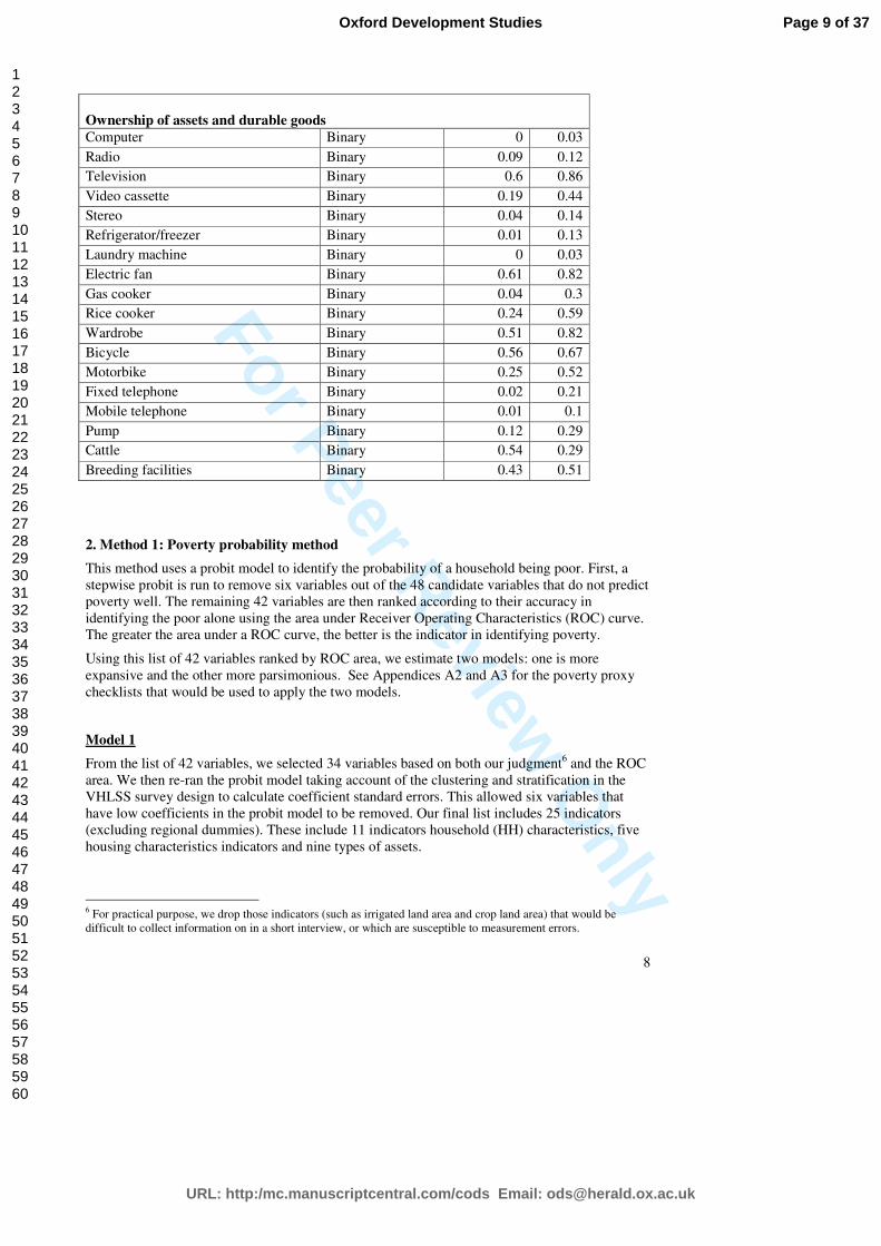
Ownership of assets and durable goods Computer Binary 0 0.03

Radio Binary 0.09 0.12

Television Binary 0.6 0.86

Video cassette Binary 0.19 0.44

Stereo Binary 0.04 0.14

Refrigerator/freezer Binary 0.01 0.13

Laundry machine Binary 0 0.03

Electric fan Binary 0.61 0.82

Gas cooker Binary 0.04 0.3

Rice cooker Binary 0.24 0.59

Wardrobe Binary 0.51 0.82

Bicycle Binary 0.56 0.67

Motorbike Binary 0.25 0.52

Fixed telephone Binary 0.02 0.21

Mobile telephone Binary 0.01 0.1

Pump Binary 0.12 0.29

Cattle Binary 0.54 0.29

Breeding facilities Binary 0.43 0.51

2. Method 1: Poverty probability method

This method uses a probit model to identify the probability of a household being poor. First, a stepwise probit is run to remove six variables out of the 48 candidate variables that do not predict poverty well. The remaining 42 variables are then ranked according to their accuracy in identifying the poor alone using the area under Receiver Operating Characteristics (ROC) curve. The greater the area under a ROC curve, the better is the indicator in identifying poverty.

Using this list of 42 variables ranked by ROC area, we estimate two models: one is more expansive and the other more parsimonious. See Appendices A2 and A3 for the poverty proxy checklists that would be used to apply the two models.

Model 1

From the list of 42 variables, we selected 34 variables based on both our judgment6 and the ROC area. We then re-ran the probit model taking account of the clustering and stratification in the VHLSS survey design to calculate coefficient standard errors. This allowed six variables that have low coefficients in the probit model to be removed. Our final list includes 25 indicators (excluding regional dummies). These include 11 indicators household (HH) characteristics, five housing characteristics indicators and nine types of assets.

6 For practical purpose, we drop those indicators (such as irrigated land area and crop land area) that would be difficult to collect information on in a short interview, or which are susceptible to measurement errors.

Page 9 of 37



123456789101112131415161718192021222324252627282930313233343536373839404142434445464748495051525354555657585960

For Peer Review O

nly

9

Table 2 presents the accuracy of these indicators in identifying the poor in rural Vietnam in terms of the area under the ROC curve for each variable. Recall that the higher is the area under an ROC curve, the better the variable underlying it is in distinguishing between the poor and non-poor. Recall that the maximum value which the area under an ROC curve is 1, and that values less than 0.5 will generally lie below the leading diagonal. Indicators with areas under the ROC curve that are significantly greater than 0.5 can be viewed as useful poverty proxies, while areas substantially less than 0.5 may be regarded as indicators of non-poverty.

Table 2: Accuracy of different indicators in identifying the poor in Vietnam

Indicators Type Area under ROC curve

Household size HH characteristics 0.605

Share of children HH characteristics 0.642

Share of working HH characteristics 0.363

Share of female HH characteristics 0.536

Head finishing primary school HH characteristics 0.499

Head finishing secondary school HH characteristics 0.457

Head finishing high school and above HH characteristics 0.459

Minority HH characteristics 0.635

Wage job HH characteristics 0.453

Non-farm self-employment HH characteristics 0.401

Semi-permanent house Housing 0.496

House with private bathroom/kitchen Housing 0.480

Electricity Housing 0.463

Flush toilet Housing 0.391

Double-vault toilet Housing 0.461

House with shared bathroom or kitchen Housing 0.458

Radio Assets 0.484

Mobile telephone Assets 0.447

Refrigerator/freezer Assets 0.434

Pump Assets 0.416

Fixed telephone Assets 0.401

Electric fan Assets 0.398

Television Assets 0.380

Video cassette Assets 0.372

Motorbike Assets 0.366

Note on Indicators: Share of children: proportion of household members less than 15 years of age. Minority: 0= all ethnic groups except Kinh and Hoa; 1= Kinh or Hoa Housing indicators: binary variables indicating if the household has these durables/facilities.

The results of the probit model are presented in Table 3. Larger household size, a higher share of women or children, and a lower share of working members are all associated with higher probability of poverty. In contrast, households with non-farm wages or non-farm self-employment have a lower probability of being poor. As expected, households whose heads belong to one of the ethnic minorities have higher probability of being poor, while the head’s education level has the opposite effect. Finally, better house type, better toilet type and the

Page 10 of 37



123456789101112131415161718192021222324252627282930313233343536373839404142434445464748495051525354555657585960

For Peer Review O

nly

10

ownership of consumer durables and fixed assets are associated with lower probabilities of being poor.

Page 11 of 37



123456789101112131415161718192021222324252627282930313233343536373839404142434445464748495051525354555657585960

For Peer Review O

nly

11

Table 3: Probit model for the composite poverty indicator (model 1)

Variables Coef. Std. Err. t-statistic

Household size 0.17 0.01 21.30

Share of children 0.74 0.06 12.85

Share of women 0.23 0.05 4.19

Share of working people -0.24 0.05 -4.92

Non-farm self-employment -0.25 0.02 -12.64

Wage jobs -0.18 0.01 -14.43

Minority 0.31 0.04 7.68

Head finishing primary school -0.18 0.03 -6.55

Head finishing secondary school -0.27 0.03 -8.96

Head finishing high school and above -0.43 0.05 -9.46

House with private bathroom/kitchen -0.57 0.05 -12.11

House with shared bathroom or kitchen -0.68 0.11 -6.14

Semi-permanent house -0.33 0.03 -10.59

Electricity 0.29 0.06 4.85

Radio -0.14 0.04 -3.94

Flush toilet -0.26 0.04 -6.60

Double-vault toilet -0.10 0.03 -3.61

Mobile telephone -0.56 0.08 -6.68

Refrigerator/freezer -0.37 0.06 -5.92

Pump -0.15 0.03 -4.87

Fixed phone -0.35 0.05 -7.45

Electric fan -0.20 0.03 -6.65

Television -0.35 0.03 -13.51

Video cassette -0.23 0.03 -8.73

Motorbike -0.40 0.03 -15.99

North East -0.24 0.04 -5.43

Central Highlands -0.32 0.07 -4.81

South East -0.58 0.06 -9.08

Mekong River Delta -0.75 0.04 -16.93

Constant -0.27 0.08 -3.34

Number of obs 33745

F(29, 2201) 121.74

Prob > F 0

Note: Some regions are removed from model because of the stepwise probit process

Figure 1 shows the ROC curve for the composite poverty indicator. As the cut-off used to distinguish the poor from the non-poor is increased, the proportion of the poor correctly identified as poor increases, along with the proportion of the non-poor who are incorrectly identified as poor. Thus the concavity of the ROC curve displays the usual trade-off between coverage of the poor and inclusion of the non-poor. The area under the ROC curve is 0.8403. This figure shows that there is a trade-off between coverage of the poor and exclusion of the non-poor in rural areas. In general, the more accurately a method is in identifying the poor, the less accurately it will be in identifying the non-poor (and vice versa).

Page 12 of 37



123456789101112131415161718192021222324252627282930313233343536373839404142434445464748495051525354555657585960

For Peer Review O

nly

12

Figure 1: ROC curve for model 1.

0.0

00

.25

0.5

00.7

51.0

0C

ove

rage

of P

oo

r (S

en

sitiv

ity)

0.00 0.25 0.50 0.75 1.00Inclusion of Non-Poor (1 - Specificity)

Area under ROC curve = 0.8403

Model 2

In the model 2, we chose a more parsimonious list of 11 household-level indicators based on several criteria including their ease of collection, their ROC area, and their coefficients and statistical significance in explaining absolute income poverty. The final list includes 4 household characteristics (share of children, minority, household size, head finishing high school), 3 accommodation characteristics (house with private bathroom/kitchen, house with shared bathroom or kitchen, flush toilet) and 4 durable ownership variables (mobile phone, electric fan, television and motorbike).

Page 13 of 37



123456789101112131415161718192021222324252627282930313233343536373839404142434445464748495051525354555657585960

For Peer Review O

nly

13

Table 4: Probit model for the composite poverty indicator (model 2)

Variables Coef. Std. Err. t-statistics

Share of children 1.05 0.05 21.30 Minority 0.44 0.04 11.06 Household size 0.10 0.01 14.77 Head finishing high school and above -0.32 0.04 -7.94 House with private bathroom/kitchen -0.49 0.10 -4.85 House with shared bathroom or kitchen -0.36 0.04 -9.82 Flush toilet -0.40 0.04 -11.19 Mobile phone -0.83 0.08 -10.32 Electric fan -0.25 0.03 -8.85 Television -0.50 0.03 -19.15 Motorbike -0.50 0.02 -20.54 North East -0.20 0.04 -4.48 Central Highlands -0.24 0.06 -3.74 South East -0.52 0.06 -8.83 Mekong River Delta -0.62 0.04 -16.35 Constant -0.51 0.04 -12.04 Number of obs 33745 F(15, 2215) 190.26 Prob > F 0

Figure 2 shows the ROC curve for model 2. The ROC area is 0.8116, less than the ROC area in Model 1 (0.8403). Thus, Model 1 performs better than Model 2 in terms of ROC areas.

Figure 2: ROC area for model 2

0.0

00.2

50.5

00

.75

1.0

0C

overa

ge

of

Po

or

(Se

nsitiv

ity)

0.00 0.25 0.50 0.75 1.00Inclusion of Non- Poor (1 - Specificity)

Area under ROC curve = 0.8116

Page 14 of 37



123456789101112131415161718192021222324252627282930313233343536373839404142434445464748495051525354555657585960

For Peer Review O

nly

14

Table 5 shows the trade-off between correct coverage of the poor and exclusion of the non-poor in rural areas at different cut-off points. The cut-off points are the predicted probability scores from the probit models in Table 3 and Table 4. If a very low value for the cut-off (such as 0.05) is chosen, nearly all the households (97.3%) would be correctly identified as poor in model 1. However, at this cut-off, only 34.6% of the non-poor would be correctly identified as non-poor in mode 1. In contrast, if a very high value for the cut-off such as 0.95 is chosen, all non-poor households would be correctly identified as non-poor but only 1.11 percent of the poor households would be correctly identified. Thus, the choice of cut-off point would depend on the relative importance that policy-makers attaches to the two objectives: (a) coverage of the poor and (b) exclusion of the non-poor.

In Table 5, the optimal cut-off points based on total accuracy (that is the proportion of all households who are correctly identify as poor or non-poor) are 0.40 for model 1 and 0.45 for model 2. At the cut-off point of 0.40, 52 percent of the poor and 90 percent of the non-poor are correctly identified in Model 1 and 45 percent of the poor and 91 percent of the non-poor are correctly identified in Model 2.

On the other hand, the optimal cut-off point based on BPAC (which give more weight to accurate identification of the poor) is 0.35 for both models. At this cut-off point, which is shown in bold in Table 5, 79.2 percent and 77.7 percent of the people are correctly identified in models 1 and 2, respectively. In addition, 59.2 percent of the poor and 86.8 percent of the non-poor are correctly identified in Model 1. For Model 2, 53.1 percent of the poor and 87.1 percent of the non-poor are correctly identified.

Comparing the two models, it is clear that Model 1 performs better than Model 2 in terms of both poverty accuracy and total accuracy. Model 1 also performs better than Model 2 at almost all cut-off points in terms of BPAC. However, Model 2 has higher BPAC than Model 1 at the optimal cut-off point. Yet, Model 2 is more susceptible to the choosing of cut-off point. For example, moving from the cut-off point of 0.4 to 0.45 reduces BPAC by 60.2 percent in Model 1 and by 77.7 percent in Model 2.

Page 15 of 37



123456789101112131415161718192021222324252627282930313233343536373839404142434445464748495051525354555657585960

For Peer Review O

nly

15

Table 5: Accuracy of the Poverty Probability Method

----------------Model 1----------------------------- ----------------Model 2 -------------------

Cut-

off

point

Poverty

accuracy

Non-

poverty

accuracy

Total

accuracy

BPAC Poverty

accuracy

Non-

poverty

accuracy

Total

accuracy

BPAC

0.05 97.32 34.63 48.20 -136.53 97.54 26.68 42.02 -165.31

0.10 92.88 49.72 59.06 -81.93 92.99 43.52 54.23 -104.35

0.15 87.56 61.07 66.80 -40.87 85.96 57.30 63.50 -54.51

0.20 81.30 70.12 72.54 -8.10 77.28 68.36 70.29 -14.47

0.25 73.90 77.07 76.38 17.02 69.29 76.62 75.04 15.41

0.30 66.75 82.46 79.06 36.55 59.75 83.20 78.12 39.21

0.35 59.15 86.81 80.82 52.29 53.11 87.07 79.71 53.02

0.40 52.01 90.28 81.99 39.21 44.71 91.21 81.14 21.23

0.45 44.86 92.85 82.46 15.61 40.13 93.23 81.74 4.74

0.50 38.06 95.09 82.74 -6.09 32.13 95.70 81.93 -20.18

0.55 32.17 96.56 82.61 -23.20 27.55 96.73 81.75 -33.06

0.60 27.02 97.69 82.39 -37.61 21.59 97.98 81.44 -49.51

0.65 22.06 98.43 81.89 -50.19 16.69 98.60 80.87 -61.56

0.70 17.82 98.99 81.42 -60.71 13.43 99.16 80.60 -70.12

0.75 13.61 99.39 80.82 -70.58 8.57 99.57 79.87 -81.30

0.80 9.70 99.75 80.25 -79.69 6.49 99.76 79.57 -86.17

0.85 5.94 99.91 79.56 -87.78 3.23 99.90 78.97 -93.19

0.90 3.07 99.98 78.99 -93.80 1.15 99.96 78.56 -97.54

0.95 1.11 100.00 78.59 -97.78 0.25 100.00 78.40 -99.51

2. Method 2: OLS regression

In this method, a stepwise OLS regression is run based on the list of candidate variables in Table 1. The dependent variable is the natural logarithm of per capita real household income in 2006 in rural Vietnam. After dropping 10 variables (including living area, total land area, and source of drinking water) that were not statistically different from zero at the 10% level have insignificant explanatory power, the results from OLS are presented in Table 6.

Page 16 of 37



123456789101112131415161718192021222324252627282930313233343536373839404142434445464748495051525354555657585960

For Peer Review O

nly

16

Table 6: OLS regression of real per capita income 2006

Coef. Std. Err. t-statistic

Household size -0.39 0.01 -29.03 Minority -0.09 0.02 -5.42 Share of working members 0.17 0.02 7.92 Share of children -0.20 0.03 -6.91 Share of women -0.12 0.02 -6.09 Non-farm self employment 0.07 0.01 13.50 Wage job 0.04 0.00 9.80 Head finishing primary school 0.06 0.01 5.96 Head finishing secondary school 0.08 0.01 7.30 Head finishing high school and above 0.14 0.01 9.79 Head’s age (logarithm) 0.06 0.02 3.46 House with private bathroom/kitchen 0.14 0.03 5.04 House with shared bathroom or kitchen

0.07 0.01 6.52

Flush toilet 0.10 0.01 7.56 Double-vault toilet 0.04 0.01 3.42 Gas cooker 0.16 0.01 13.46 Wardrobe 0.11 0.01 10.74 Fixed phone 0.11 0.01 8.51 Television 0.10 0.01 8.52 Motorbike 0.14 0.01 16.22 Video cassette 0.08 0.01 9.33 Rice cooker 0.07 0.01 8.15 Electric fan 0.04 0.01 3.68 Mobile phone 0.21 0.01 13.98 Laundry 0.17 0.03 4.83 Refrigerator/freezer 0.17 0.02 11.08 Pump 0.03 0.01 3.64 Cattle -0.05 0.01 -5.33 North East 0.11 0.02 6.64 Central Highlands 0.17 0.03 6.80 South East 0.13 0.02 6.55 Mekong River Delta 0.28 0.02 17.52 Constant 8.15 0.08 101.67 Number of obs 24815 F( 32, 2186) 295.9 Prob > F 0 R-squared 0.46

From the OLS regression, it is possible to predict household per capita income. Then by comparing predicted per capita income with the poverty line, each household’s poverty status can be predicted. Table 7 shows the tabulation between predicted and actual poverty status using OLS regression and an absolute poverty line of $1.25/day. 36.8 percent of the poor and 95.7 percent of the non-poor are correctly identified using the absolute poverty line of $1.25 per day.

Page 17 of 37



123456789101112131415161718192021222324252627282930313233343536373839404142434445464748495051525354555657585960

For Peer Review O

nly

17

Table 7: Predicted and actual poverty using absolute poverty line (OLS regression)

Predicted non-poor Predicted poor

Actual non-poor 95.71 4.29

Actual poor 63.32 36.68

Poverty accuracy 36.68

Total accuracy 83.49

BPAC 48.82

The BPAC for Method 2 is equal to 48.82, lower than the corresponding figure for Method 1.

For further comparison between Method 1 and Method 2, we estimate the probability of households being poor from the OLS regression. The probability of a household being poor is given as

)ln

{'

*

σ

βii

XzP

−Φ= where z is the poverty line ($1.25), Φ is the cumulative standard normal

distribution and σ is the standard error of the residuals (Hentschel et al., 2000). Table 8 presents the accuracy in identifying poverty based on the poverty line of $1.25 and the estimated poverty probability. BPAC is maximized at the cut-off point of 0.35 (again shown in bold). At that point, 58 percent of the poor and 87.6 percent of the non-poor are correctly identified.

Generally, the OLS method is quite good in identifying poverty. Another advantage of the OLS method over the probit models is that it can predict the incomes of particular households, thus enable calculate such income-based poverty statistics as poverty gap and poverty severity. However, the standard errors associated with such poverty measures at the household level are typically very large.

Page 18 of 37



123456789101112131415161718192021222324252627282930313233343536373839404142434445464748495051525354555657585960

For Peer Review O

nly

18

Table 8: Poverty identification accuracy- OLS method

Cut-off points

Poverty accuracy

Non- poverty accuracy

Total accuracy

BPAC

0.05 97.43 30.82 44.61 -165.07

0.10 93.83 47.07 56.75 -102.81

0.15 88.01 58.95 64.97 -57.28

0.20 81.04 69.41 71.82 -17.20

0.25 74.46 77.27 76.69 12.91

0.30 65.97 82.98 79.46 34.78

0.35 57.95 87.64 81.49 52.63

0.40 50.00 91.19 82.66 33.75

0.45 43.38 93.76 83.34 10.66

0.50 36.68 95.71 83.50 -10.21

0.55 30.16 97.28 83.39 -29.25

0.60 24.09 98.33 82.96 -45.42

0.65 18.11 99.02 82.28 -60.04

0.70 13.21 99.47 81.62 -71.54

0.75 8.52 99.82 80.92 -82.26

0.80 5.38 99.89 80.33 -88.83

0.85 2.64 99.99 79.84 -94.66

0.90 0.79 100.00 79.47 -98.41

0.95 0.10 100.00 79.32 -99.81

3. Method 3: Principal Component Analysis

The third method we use is principal component analysis (PCA). Principal component analysis is a technique for reducing the information contained in a large set of variables to a smaller number. The first principal component is the linear index of the underlying variables that captures the most variation among them (Filmer and Pritchett, 2001). The method has been applied extensively in the education and health literature in other countries (Filmer and Prichett, 2001; Rutstein and Rubin, 2004) and in several unpublished papers which estimate an “asset index” for Vietnamese households (Gwatkin et al. 2007, Chowdhuri and Baulch, 2010).

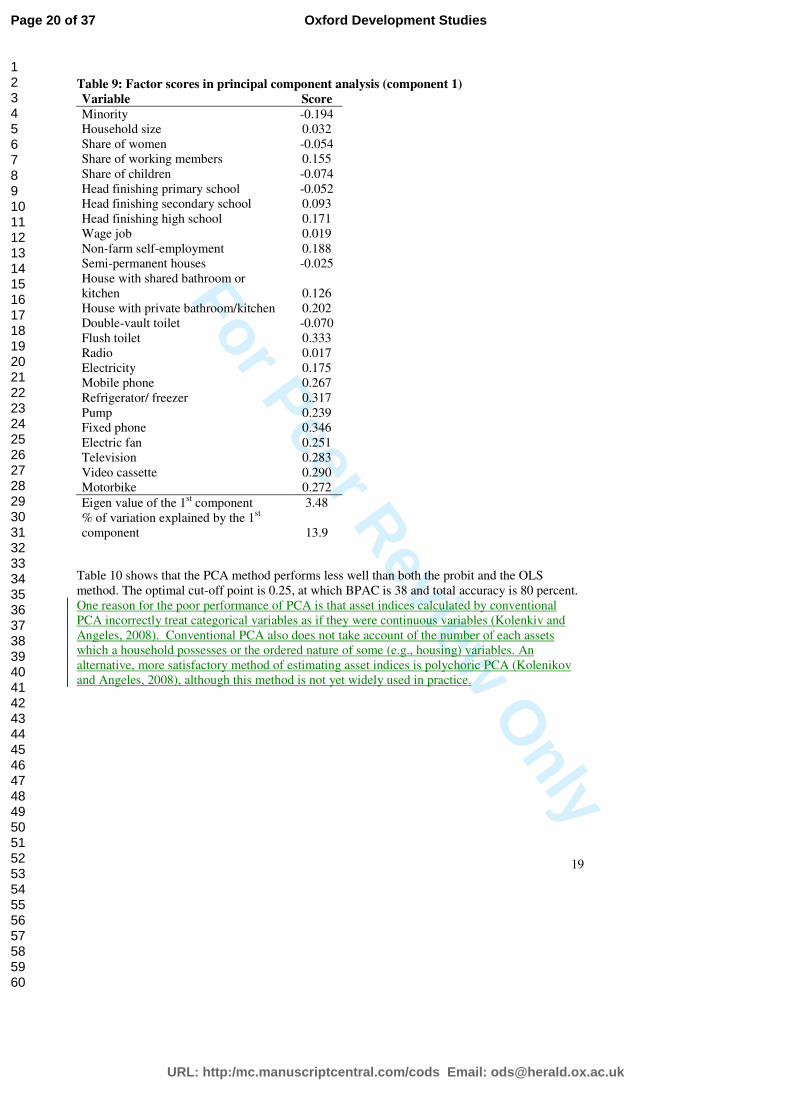
For the sake of simplicity, we use the same set of variables as in Method 1(Model 1) for our PCA. Table 9 shows the factor scores associated with these variables. Generally, a variable with a positive factor score is associated with higher socio-economic status, while a variable with a negative factor score is associated with lower socio-economic status. Using the factor scores from the first principal components as the weights, we then construct an asset index for each household which has a mean equal to zero and a standard deviation equal to one. Table 10 shows the accuracy from this method, using percentiles of asset index as cut-off points.

Deleted: Sahn and Stiffel, 2003;

Page 19 of 37



123456789101112131415161718192021222324252627282930313233343536373839404142434445464748495051525354555657585960

For Peer Review O

nly

19

Table 9: Factor scores in principal component analysis (component 1) Variable Score Minority -0.194 Household size 0.032 Share of women -0.054 Share of working members 0.155 Share of children -0.074 Head finishing primary school -0.052 Head finishing secondary school 0.093 Head finishing high school 0.171 Wage job 0.019 Non-farm self-employment 0.188 Semi-permanent houses -0.025 House with shared bathroom or kitchen 0.126 House with private bathroom/kitchen 0.202 Double-vault toilet -0.070 Flush toilet 0.333 Radio 0.017 Electricity 0.175 Mobile phone 0.267 Refrigerator/ freezer 0.317 Pump 0.239 Fixed phone 0.346 Electric fan 0.251 Television 0.283 Video cassette 0.290 Motorbike 0.272

Eigen value of the 1st component 3.48 % of variation explained by the 1st component 13.9

Table 10 shows that the PCA method performs less well than both the probit and the OLS method. The optimal cut-off point is 0.25, at which BPAC is 38 and total accuracy is 80 percent. One reason for the poor performance of PCA is that asset indices calculated by conventional PCA incorrectly treat categorical variables as if they were continuous variables (Kolenkiv and Angeles, 2008). Conventional PCA also does not take account of the number of each assets which a household possesses or the ordered nature of some (e.g., housing) variables. An alternative, more satisfactory method of estimating asset indices is polychoric PCA (Kolenikov and Angeles, 2008), although this method is not yet widely used in practice.

Page 20 of 37



123456789101112131415161718192021222324252627282930313233343536373839404142434445464748495051525354555657585960

For Peer Review O

nly

20

Table 10: Accuracy of the PCA method

Cut-off points

Asset index

Poverty accuracy

Non-Poverty accuracy

Total accuracy

BPAC

0.05 -2.55 14.39 97.59 79.58 -62.52

0.10 -2.02 26.58 94.58 79.86 -27.23

0.15 -1.66 37.11 91.11 79.41 6.39

0.20 -1.36 46.28 87.26 78.39 38.65

0.25 -1.11 54.56 83.16 76.96 39.06

0.30 -0.89 61.89 78.81 75.15 23.34

0.35 -0.69 68.10 74.14 72.83 6.45

0.40 -0.49 73.89 69.36 70.34 -10.85

0.45 -0.29 78.51 64.26 67.34 -29.32

0.50 -0.10 82.63 59.02 64.13 -48.29

0.55 0.11 86.40 53.68 60.76 -67.61

0.60 0.33 89.36 48.11 57.04 -87.75

0.65 0.58 92.17 42.51 53.26 -108.03

0.70 0.84 94.63 36.81 49.33 -128.65

0.75 1.17 96.31 30.88 45.05 -150.08

0.80 1.59 97.70 24.89 40.66 -171.76

0.85 2.12 98.77 18.80 36.12 -193.79

0.90 2.83 99.42 12.60 31.40 -216.24

0.95 3.83 99.88 6.35 26.60 -238.87

4. Method 4: Quantile regression

The fourth method we consider is quantile regression. This method is recommended by IRIS Center (2008) as the most suitable method in Vietnam using a poverty cut-off corresponding to the 50 percentile of the expenditure distribution. For comparability, we use the same set of variables in the quantile regressions as in Model 1 of the poverty probability model and the PCA. However, unlike the IRIS centre we ran the regression with the quantile approximating to the $1.25/day poverty line (0.22). 7 Table 11 reports results from the quantile regression at the 22nd percentile while Table 12 shows the accuracy of the method.

7 We thank an anonymous reviewer for this suggestion. Note that we have also run this regression with the quantile corresponding to the median, and the results are similar to those with the 22nd percentile.

Page 21 of 37



123456789101112131415161718192021222324252627282930313233343536373839404142434445464748495051525354555657585960

For Peer Review O

nly

21

Table 11: Quantile regression

Coef. Std. Err. t-statistic

Household size -0.08 0.00 -30.87 Share of children -0.27 0.02 -12.88 Share of women -0.06 0.02 -2.77 Share of working people 0.14 0.02 7.93 Non-farm self-employment 0.09 0.00 18.25 Wage jobs 0.08 0.00 21.22 Minority -0.12 0.01 -9.53 Head finishing primary school 0.06 0.01 6.71 Head finishing secondary school 0.09 0.01 8.86 Head finishing high school and above 0.18 0.01 13.06 House with private bathroom/kitchen 0.27 0.02 11.52 House with shared bathroom or kitchen 0.20 0.01 14.01 Semi-permanent house 0.14 0.01 13.52 Electricity -0.09 0.02 -5.33 Radio 0.06 0.01 5.17 Flush toilet 0.13 0.01 11.06 Double-vault toilet 0.05 0.01 5.12 Mobile telephone 0.23 0.01 15.45 Refrigerator/freezer 0.17 0.01 12.66 Pump 0.06 0.01 6.76 Fixed phone 0.14 0.01 12.58 Electric fan 0.08 0.01 7.94 Television 0.14 0.01 13.36 Video cassette 0.09 0.01 10.80 Motorbike 0.16 0.01 19.39 North East 0.11 0.01 9.58 Central Highlands 0.15 0.02 8.61 South East 0.19 0.01 13.79 Mekong River Delta 0.29 0.01 26.99 Constant 7.74 0.03 286.26

Table 12 evaluates the accuracy of the quantile regression method. With a cut-off point of 0.25, the quantile regression method identifies 62 percent of the poor and 85 percent of the non-poor correctly, resulting in a total accuracy of 80 percent. The BPAC for the quantile regression method is 46.5, which is substantially lower than those for the poverty probability and OLS models.

Page 22 of 37



123456789101112131415161718192021222324252627282930313233343536373839404142434445464748495051525354555657585960

For Peer Review O

nly

22

Table 12: Accuracy of the quantile regression method

Cut-off points

Poverty accuracy

Non-Poverty

accuracy

Total accuracy

BPAC

0.05 18.83 98.82 81.50 -58.08 0.10 32.85 96.31 82.57 -20.96 0.15 44.01 93.01 82.40 13.30 0.20 53.74 89.32 81.62 46.10 0.25 61.94 85.21 80.17 46.47 0.30 69.09 80.80 78.26 30.53 0.35 75.13 76.09 75.88 13.48 0.40 80.20 71.10 73.07 -4.57 0.45 84.09 65.80 69.76 -23.74 0.50 87.89 60.47 66.41 -43.04 0.55 90.73 54.87 62.64 -63.28 0.60 93.17 49.17 58.69 -83.93 0.65 95.34 43.38 54.64 -104.85 0.70 96.64 37.36 50.20 -126.64 0.75 98.02 31.36 45.79 -148.35 0.80 98.92 25.23 41.18 -170.55 0.85 99.47 19.00 36.42 -193.08 0.90 99.72 12.69 31.53 -215.93 0.95 99.96 6.37 26.64 -238.77

To conclude this section, we present a tabular and graphical comparison of the four poverty proxy approaches. Table 13 compares these four approaches at their optimal cut-points. The quantile regression approach has the highest poverty accuracy, while OLS has the highest non-poverty accuracy. However, judged in terms of total accuracy, the OLS approach has the best result, followed by the probit model 1. If BPAC, which is our preferred measure is used, the Probit Model 1, Probit Model 2 and OLS produce similar results, while those for PCA and quantile regression approaches are substantially lower. The PCA approach has both the lowest total accuracy and BPAC.

Table 13: Comparing the accuracy of the four approaches

Cut-off points

Poverty accuracy

Non-Poverty accuracy

Total accuracy

BPAC

Probit: Model 1 (enlarge) 0.35 59.15 86.81 80.82 52.29

Probit: Model 2 (parsimonious)

0.35 53.11 87.07 79.71 53.02

OLS 0.35 57.95 87.64 81.49 52.63

PCA 0.25 54.56 83.16 76.96 39.06

Quantile regression 0.25 61.94 85.21 80.17 46.47

Page 23 of 37



123456789101112131415161718192021222324252627282930313233343536373839404142434445464748495051525354555657585960

For Peer Review O

nly

23

Figure 3 summarizes the ROC areas under four approaches, using 20 cut-off points for each model described above. The probit Model 1, OLS regression and the quantile regression have very similar ROC areas, and their ROC curves are visually (and statistically) indistinguishable from one another. This confirms these three models’ performance using the BPAC. In contrast, probit Model 2 and the PCA method have lower ROC curves and areas, with PCA having the lowest area under the ROC curve. This confirms the PCA methods poor performance according to the BPAC.

Finally, we report the poverty headcount ratios, as calculated by four models at the optimal points. Poverty rates are defined as the percentage of households who are considered poor at the optimal cut-off points to the total population. The standard errors of the poverty rates are calculated based on bootstrapping with 200 replications. The results are presented in Table 14. Table 14 shows that Model 1 slightly overestimates the true poverty rate while the other models underestimate it. The 95% confidence intervals show that the Probit Model 1 and OLS estimates of the poverty headcount ratio are not statistically different from the “true” poverty headcount ratio estimated directly from the VHLSS06.

Page 24 of 37



123456789101112131415161718192021222324252627282930313233343536373839404142434445464748495051525354555657585960

For Peer Review O

nly

24

Table 14: Poverty headcount ratios and standard errors the four approaches

Poverty headcount

Ratio

Bootstrapped standard errors

95% confidence interval

Probit: Model 1 23.14 0.50 22.28 24.00

Probit: Model 2 21.63 0.41 20.85 22.31

OLS 21.80 0.50 20.88 22.72

PCA 20.00 0.27 22.14 23.10

Quantile regression 20.00 0.28 19.45 20.55

"True" poverty headcount ratio 22.36

From this analysis, we choose the probit method with Model 1 as our preferred model, as it performs well in terms of Total Accuracy, the BPAC, the area under the ROC curve and in predicting the poverty headcount. In the next section, we will validate this model by testing its robustness to different poverty lines and an alternative household datasets.

Figure 3: Areas under the ROC curve for the four approaches

0.0

00.2

50.5

00

.75

1.0

0C

overa

ge o

f P

oor

(Sen

sitiv

ity)

0.00 0.25 0.50 0.75 1.00Inclusion of Non-Poor (1-Specificity)

Probit Model 1: 0.8353 Probit Model 2: 0.8047

OLS: 0.8355 PCA: 0.7781

Quantile Regression: 0.8346 Reference

5. Validating the Poverty Probability Method

To validate the use of the poverty probability method, we conduct three exercises: using two different poverty lines with the same dataset (VHLSS06), and using an alternative household

Page 25 of 37



123456789101112131415161718192021222324252627282930313233343536373839404142434445464748495051525354555657585960

For Peer Review O

nly

25

datasets (the VHLSS04) to test its robustness. As Chen and Schreiner (2009) and others have pointed-out, it is important to know about the out-of-sample predictive power of an approach since an approach which identifies the poor very accurately with one dataset may perform poorly when applied to different data.

5.1. Validating using a moderate poverty line

We tested our preferred model (Model 1, probit) with the higher international income poverty line of $2 per capita per day, which is used to identify the moderately poor (Chen and Ravallion, 2008). . The results in Table 15 show that the model is rather good at predicting both extreme and moderate poverty. At the cut-off point of 0.50, the model correctly identifies 75.6 percent of the poor and 73.2 percent of the non-poor. Overall, the poverty status of 74.4 percent of all households is correctly identified, while the BPAC is relatively high at 72.4.

Table 15: Accuracy of Poverty Probability Method with $2/day Poverty Line

Cut-off points

Poverty accuracy

Non-poverty accuracy

Total accuracy

BPAC

0.05 99.56 12.31 55.36 9.95

0.10 98.66 20.38 59.00 18.25

0.15 97.54 27.58 62.10 25.63

0.20 95.98 34.41 64.78 32.65

0.25 94.04 41.65 67.50 40.08

0.30 91.68 48.15 69.62 46.75

0.35 88.69 54.97 71.61 53.76

0.40 85.17 61.07 72.96 60.02

0.45 80.93 67.35 74.05 66.47

0.50 75.60 73.14 74.35 72.42

0.55 69.58 78.48 74.09 61.26

0.60 62.91 83.38 73.28 42.89

0.65 55.51 87.88 71.91 23.46

0.70 47.58 91.53 69.85 3.85

0.75 39.24 94.64 67.30 -16.01

0.80 31.26 96.79 64.46 -34.18

0.85 22.57 98.39 60.98 -53.20

0.90 14.81 99.28 57.61 -69.64

0.95 7.24 99.86 54.17 -85.38

Page 26 of 37



123456789101112131415161718192021222324252627282930313233343536373839404142434445464748495051525354555657585960

For Peer Review O

nly

26

1.2. Validating using a consumption-based poverty line

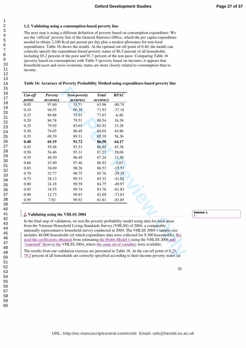
The next step is using a different definition of poverty based on consumption expenditure. We use the ‘official’ poverty line of the General Statistics Office, which the per capita expenditure needed to obtain 2,100 Kcal per person per day plus a modest allowance for non-food expenditures. Table 16 shows the results. At the optimal cut-off point of 0.40, the model can correctly specify the expenditure-based poverty status of 86.5 percent of all households, including 65.2 percent of the poor and 91.7 percent of the non-poor. Comparing Table 16 (poverty based on consumption) with Table 5 (poverty based on income), it appears that household asset and socio-economic status are more closely related to consumption than to income.

Table 16: Accuracy of Poverty Probability Method using expenditure-based poverty line

Cut-off

points

Poverty

accuracy

Non-poverty

accuracy

Total

accuracy

BPAC

0.05 97.60 55.71 63.96 -80.74

0.10 94.55 66.39 71.93 -37.16

0.15 89.88 73.93 77.07 -6.40

0.20 84.78 79.51 80.54 16.38

0.25 79.92 83.65 82.92 33.28

0.30 74.05 86.49 84.04 44.86

0.35 69.39 89.31 85.39 56.36

0.40 65.19 91.72 86.50 64.17

0.45 59.48 93.53 86.82 45.38

0.50 54.46 95.31 87.27 28.06

0.55 49.50 96.49 87.24 13.30

0.60 43.90 97.46 86.92 -1.83

0.65 38.69 98.26 86.53 -15.51

0.70 32.77 98.75 85.76 -29.35

0.75 28.13 99.33 85.32 -41.02

0.80 24.18 99.59 84.75 -49.97

0.85 18.55 99.74 83.76 -61.83

0.90 12.73 99.83 82.69 -73.83

0.95 7.92 99.92 81.81 -83.85

2. Validating using the VHLSS 2004

In the final step of validation, we test the poverty probability model using data for rural areas from the Vietnam Household Living Standards Survey (VHLSS) of 2004, a comparable nationally representative household survey conducted in 2004. The VHLSS 2004’s sample size includes 46,000 households (of which expenditure data were collected for 9,300 households). We used the coefficients obtained from estimating the Probit Model 1 using the VHLSS 2006 and “exported” these to the VHLSS 2004, where the same set of variables were available.

The results from our validation exercise are presented in Table 18. At the cut-off point of 0.25, 79.2 percent of all households are correctly specified according to their income poverty status (at

Deleted: ¶3

Page 27 of 37



123456789101112131415161718192021222324252627282930313233343536373839404142434445464748495051525354555657585960

For Peer Review O

nly

27

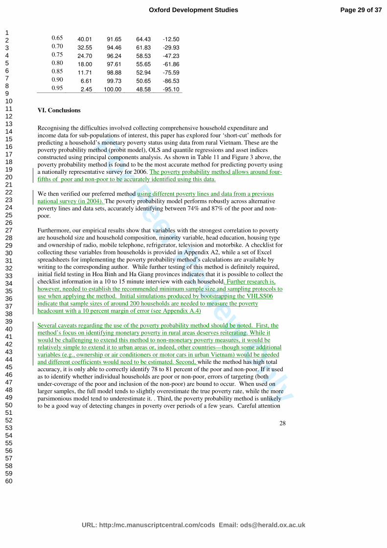
$1.25 per head), including 52.8 percent of the poor and 86.9 percent of the non-poor. The BPAC is 50.4We also test the model with the moderate international poverty line of $2 per capita in Table 19. The results show that the model performs well. At the cut-off point of 0.4, 70.9 percent of all households are correctly classified, including 75.5 percent of the poor and 65.8 percent of the non-poor. The BPAC is high at 69.3. Table 18: Accuracy of Poverty Probability Method using VHLSS 2004 and $1.25/day line

Cut-off

points

Poverty

accuracy

Non-poor

accuracy

Total

accuracy

BPAC

0.05 91.32 43.31 54.17 -93.87 0.10 81.48 61.41 65.95 -31.97 0.15 71.86 72.88 72.65 7.27 0.20 61.71 81.55 77.06 36.92 0.25 52.79 86.89 79.18 50.40 0.30 43.86 90.91 80.27 18.80

0.35 37.25 93.90 81.08 -4.66

0.40 30.38 95.55 80.81 -24.02

0.45 23.86 97.01 80.46 -42.07

0.50 18.24 98.08 80.01 -56.94

0.55 14.41 98.78 79.69 -67.00

0.60 10.70 99.38 79.31 -76.47

0.65 7.32 99.75 78.84 -84.51

0.70 5.05 99.86 78.41 -89.43

0.75 2.72 99.91 77.92 -94.24

0.80 1.26 99.92 77.60 -97.21

0.85 0.60 100.00 77.51 -98.79

0.90 0.42 100.00 77.47 -99.16

0.95 . . . .

Table 19: Accuracy of Poverty Probability Method using VHLSS 2004 and $2/day line

Cut-off

points

Poverty

accuracy

Non-

poor

accuracy

Total

accuracy

BPAC

0.05 99.62 7.38 56.00 16.89 0.10 98.40 16.83 59.82 25.37

0.15 96.36 25.99 63.08 33.60

0.20 93.67 34.66 65.76 41.37

0.25 90.31 43.10 67.98 48.94 0.30 86.32 51.80 69.99 56.75

0.35 81.10 59.41 70.85 63.58

0.40 75.50 65.75 70.89 69.27

0.45 69.94 73.13 71.45 64.00 0.50 62.92 78.45 70.26 45.17

0.55 55.20 83.33 68.50 25.35

0.60 47.27 88.02 66.54 5.28

Deleted: 4

Deleted: 3

Deleted: .

Deleted: ¶

Page 28 of 37



123456789101112131415161718192021222324252627282930313233343536373839404142434445464748495051525354555657585960

For Peer Review O

nly

28

0.65 40.01 91.65 64.43 -12.50

0.70 32.55 94.46 61.83 -29.93

0.75 24.70 96.24 58.53 -47.23 0.80 18.00 97.61 55.65 -61.86

0.85 11.71 98.88 52.94 -75.59

0.90 6.61 99.73 50.65 -86.53

0.95 2.45 100.00 48.58 -95.10

VI. Conclusions

Recognising the difficulties involved collecting comprehensive household expenditure and income data for sub-populations of interest, this paper has explored four ‘short-cut’ methods for predicting a household’s monetary poverty status using data from rural Vietnam. These are the poverty probability method (probit model), OLS and quantile regressions and asset indices constructed using principal components analysis. As shown in Table 11 and Figure 3 above, the poverty probability method is found to be the most accurate method for predicting poverty using a nationally representative survey for 2006. The poverty probability method allows around four-fifths of poor and non-poor to be accurately identified using this data. We then verified our preferred method using different poverty lines and data from a previous national survey (in 2004). The poverty probability model performs robustly across alternative poverty lines and data sets, accurately identifying between 74% and 87% of the poor and non-poor. Furthermore, our empirical results show that variables with the strongest correlation to poverty are household size and household composition, minority variable, head education, housing type and ownership of radio, mobile telephone, refrigerator, television and motorbike. A checklist for collecting these variables from households is provided in Appendix A2, while a set of Excel spreadsheets for implementing the poverty probability method’s calculations are available by writing to the corresponding author. While further testing of this method is definitely required, initial field testing in Hoa Binh and Ha Giang provinces indicates that it is possible to collect the checklist information in a 10 to 15 minute interview with each household. Further research is, however, needed to establish the recommended minimum sample size and sampling protocols to use when applying the method. Initial simulations produced by bootstrapping the VHLSS06 indicate that sample sizes of around 200 households are needed to measure the poverty headcount with a 10 percent margin of error (see Appendix A.4) Several caveats regarding the use of the poverty probability method should be noted. First, the method’s focus on identifying monetary poverty in rural areas deserves reiterating. While it would be challenging to extend this method to non-monetary poverty measures, it would be relatively simple to extend it to urban areas or, indeed, other countries—though some additional variables (e.g., ownership or air conditioners or motor cars in urban Vietnam) would be needed and different coefficients would need to be estimated. Second, while the method has high total accuracy, it is only able to correctly identify 78 to 81 percent of the poor and non-poor. If it used as to identify whether individual households are poor or non-poor, errors of targeting (both under-coverage of the poor and inclusion of the non-poor) are bound to occur. When used on larger samples, the full model tends to slightly overestimate the true poverty rate, while the more parsimonious model tend to underestimate it. . Third, the poverty probability method is unlikely to be a good way of detecting changes in poverty over periods of a few years. Careful attention

Page 29 of 37



123456789101112131415161718192021222324252627282930313233343536373839404142434445464748495051525354555657585960

For Peer Review O

nly

29

should be given to the standard errors of the poverty rates produced, which as mentioned above are quite wide. It would also be useful to investigate how estimated coefficients of the underlying model change over time, which is possible in Vietnam due to the biennual frequency of its national household surveys. Finally, further field testing of the poverty proxy checklist and the Excel worksheets which accompany it are needed before the method can be firmly recommended for ex ante and ex post poverty impact work.

Page 30 of 37



123456789101112131415161718192021222324252627282930313233343536373839404142434445464748495051525354555657585960

For Peer Review O

nly

30

References

Alkire, S. and M.E. Santos (2010) Acute multidimensional poverty: a new index for developing countries, Human Development Research Paper 2010/11, New York: United Nations Development Program.

Baulch, B. (2002) Poverty monitoring and targeting using ROC curves: Examples from Vietnam, IDS Working Paper No. 161, http://www.ids.ac.uk/ids/bookshop/wp/wp161.pdf.

Chen, S. and M. Ravallion (2008) The developing world is poorer than we thought, but no less successful in the fight against poverty, Policy Research Working Paper Series 4703, World Bank, Washington, DC.

Chen, S. and M. Schreiner (2009) A simple poverty scorecard for Vietnam, Progress Out of Poverty, Grameen Foundation. http://www.microfinance.com/#Vietnam.

Chowdhuri. R. and Baulch, B. (2010) Should PI use an asset based approach for its poverty analysis?, Mimeo, Prosperity Initiative, Hanoi

Filmer, D. and L. Pritchett (2001) Estimating wealth effects without income or expenditure data -- or tears: an application to educational enrollments in states of India, Demography 38(1), pp. 115-132

Gwatkin, D., S. Rutstein, K. Johnson, E. Suliman, A. Wagstaff and A. Amouzou. (2007) Socio-economic differences in health, nutrition, and population: Vietnam, Country Reports on HNP and Poverty, Washington, D.C.; World Bank, http://siteresources.worldbank.org/INTPAH/Resources/400378-178119743396/vietnam.pdf.

IRIS Center (2007) Client assessment survey—Vietnam, online at http://www.povertytools.org/USAID_documents/Tools/Current_Tools/USAID_PAT_VIET_7-2007.xls.

IRIS Center (2008) Accuracy results for 20 poverty assessment tool countries, online at http://www.povertytools.org/other_documents/PAT_20_country_accuracy_results_Dec2008.pdf.

Kolenikov, S. and G. Angeles (2008), Socioeconomic status measurement with discrete proxy variables: is principal components analysis a reliable answer?, Review of Income and Wealth, 55(1), pp. 128-165.

Nguyen, Linh (2007) Identifying poverty predictors using household living standards surveys in Viet Nam, in G. Sugiyarto (ed.) Poverty Impact Analysis Selected Tools and Applications, Asian Development Bank, Manila, Philippines.

Ravallion, M., S. Chen and P. Sangraula (2008) Dollar a day revisited, Policy Research Working

Paper Series 4620, World Bank., Washington, DC.

Rustein, S. and Johnson, K. (2004) The DHS Wealth Index, DHS Comparative Reports 6, Calverton: ORC Macro

Sahn, D. and D. Stifel. (2003) Exploring alternative measures of welfare in the absence of expenditure data, Review of Income and Wealth, 49(4), pp. 463–489.

Wodon, Q. (1997) Targeting the poor using ROC curves, World Development, 25(12), pp. 2083-2092.

Page 31 of 37



123456789101112131415161718192021222324252627282930313233343536373839404142434445464748495051525354555657585960

http://www.microfinance.com/#Vietnam

For Peer Review O

nly

31

Appendices

A1. Comparison of poverty/asset indicators used by different studies in Vietnam

IRIS Sahn & Stifel Baulch

Gwatkin et al.

Chen & Schreiner Linh N.

This paper

Household characteristics

Composition

Household size √ √ √

Number of children √ √ √

Number of women √ √

% of dependents √

% of working age members √

% of working in agriculture √

Head

Head’s age √ √

Head’s marital status √

Head ethnicity √ √ √

Education

Head's education √ √ √

Spouse’s education √ Number of adults with no education √

Occupation

Agriculture activities √ √ √

Wage activities √

Non-farm activities √

Crop activities √

Agricultural services √

Accommodation and land

Type of house √ √ √

Type of roof √ √

Type of toilet √ √ √ √ √ √

Type of floor √ √ √

Source of lighting √ √ √ √

Main cooking fuel √ √

Source of drinking water √ √ √

Living area √

Number of rooms occupied √ Number of people per bedroom √

Land area √ √

Land rented out √

Page 32 of 37



123456789101112131415161718192021222324252627282930313233343536373839404142434445464748495051525354555657585960

For Peer Review O

nly

32

Assets and durables goods

Television √ √ √ √ √

Refrigerator √ √ √ √ √

Motorcycle and/or car √ √ √ √ √ √ √

Radio √ √ √ √ √

Cookers (or stoves) √ √

Bicycle √ √

Motor scooter √

Boat √

Washing machine √

Video cassette √ √

Fixed telephone √ √

Mobile telephone √

Ploughing machines √

Sewing machine √

Wardrobe √

Mill √

Garden √

Electric fan √

Pump √

# of chickens owned √

Geographic Region √ √

Page 33 of 37



123456789101112131415161718192021222324252627282930313233343536373839404142434445464748495051525354555657585960

For Peer Review O

nly

33

Appendix A2: A Poverty Proxy Checklist for Rural Vietnam (Expanded Module)

Household ID:

Date of interview: _ _ / _ _ / _ _ _ _ Length of Interview: minutes

Household head's name: Interviewer's name:

Village: Commune:

District: Province:

Please put numbers to answers

1 How many people are there living in your household?

2 How many household members…

are 14 years old or younger?

are from 15 to 59 year years old?

3 How many household members are female?

4 In the past 12 months, how many household members

work for wages/salaries

are self-employed

Please write 1 if the answer is YES, 0 if the answer is NO

5 Does the household’s head belong to an ethnic minority (not Kinh or Hoa)?

6 What is the highest education level completed by the household's head

A. Less than primary

B. Primary

C. Secondary

D. High school or above

7 What type is the household's main residence?

A. Villa or private house

B. House with a shared kitchen or bathroom/toilet

C. Semi-permanent house

D. Makeshift or other

8 Is electricity used as the main lighting in the household?

9 What type of toilet arrangement does the household have?

A. Flush toilet or sulabh toilet *

B. Double vault compost latrine or toilet directly over the water

C. No toilet or others

10 Does the household have a radio or radio cassette player?

11 Does the household have a motorbike?

12 Does the household have a fixed telephone?

13 Does the household have a mobile telephone?

14 Does the household have a television?

15 Does the household have a refrigerator/freezer?

16 Does the household have a video cassette?

17 Does the household have an electric fan?

18 Does the household have a pump? *Note: Sulabh toilets (hố xí thấm dội nước) are latrines with open bottoms, which disintegrate stools by water pouring and absorbing.

Page 34 of 37



123456789101112131415161718192021222324252627282930313233343536373839404142434445464748495051525354555657585960

For Peer Review O

nly

34

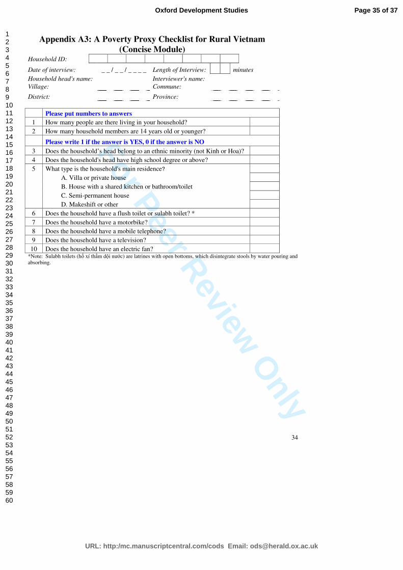
Appendix A3: A Poverty Proxy Checklist for Rural Vietnam (Concise Module)

Household ID:

Date of interview: _ _ / _ _ / _ _ _ _ Length of Interview: minutes

Household head's name: Interviewer's name:

Village: Commune:

District: Province:

Please put numbers to answers

1 How many people are there living in your household?

2 How many household members are 14 years old or younger?

Please write 1 if the answer is YES, 0 if the answer is NO

3 Does the household’s head belong to an ethnic minority (not Kinh or Hoa)?

4 Does the household's head have high school degree or above?

5 What type is the household's main residence?

A. Villa or private house

B. House with a shared kitchen or bathroom/toilet

C. Semi-permanent house

D. Makeshift or other

6 Does the household have a flush toilet or sulabh toilet? *

7 Does the household have a motorbike?

8 Does the household have a mobile telephone?

9 Does the household have a television?

10 Does the household have an electric fan? *Note: Sulabh toilets (hố xí thấm dội nước) are latrines with open bottoms, which disintegrate stools by water pouring and absorbing.

Page 35 of 37



123456789101112131415161718192021222324252627282930313233343536373839404142434445464748495051525354555657585960

For Peer Review O

nly

35

A4. Sample Size Simulations

A question arising in the poverty proxy checklist method is a suitable sample size to estimate poverty. To check this, we implemented a bootstrapping simulation based on a subset of VHLSS 2006, which include two provinces in North-Western Vietnam which are of particular interest to PI: Thanh Hoa and Hoa Binh. This subset of the VHLSS06 includes 1620 households

In the simulation, we drew n number of households from the data, and estimated poverty rate based on the subsamples, with 500 replications for each approach. We use the standard error ratio, that is the standard error of the poverty rate estimated by each of the four approach expressed as a percentage of “true” poverty rate, to determine the extend of error

The results in Table A4.1 show that if we draw less than 12% of the sample (200 households), the standard error ratio as percentage of true poverty rate is about 10.2%. If we want to achieve less than 5% standard error ratio, the sample size must be above 50% of the whole sample.

Table A4.1: Comparing sensitivity of poverty estimates to sample sizes by different approach

Standard Error Ratio (%) Sample

Size (households) Probit 1 OLS PCA

Quantile regression

5 52.19 47.97 54.26 47.05

10 43.12 43.62 50.59 41.90

20 32.34 34.69 42.52 30.81

40 23.28 25.77 30.3 21.68

60 19.56 21.48 23.27 18.14

80 16.51 19.95 21.06 15.55

100 15.08 16.69 19.04 14.12

150 12.07 13.06 16.07 11.21

200 10.19 11.19 13.7 9.42

250 9.28 10.09 12.46 8.48

300 8.54 9.17 10.99 7.76

400 7.43 7.76 9.78 6.65

500 6.62 6.92 8.5 5.95

750 5.39 5.58 7.34 4.76

1000 4.57 4.87 6.36 4.05

1500 3.6 3.91 5.23 3.27

As shown in Table A4.1 below, the standard error ratio for each of the four poverty proxy approaches falls dramatically until sample sizes of around 60 households are reached. Thereafter, although the standard error ratio continues to decline it does so at a declining rate.

Page 36 of 37



123456789101112131415161718192021222324252627282930313233343536373839404142434445464748495051525354555657585960

For Peer Review O

nly

36

Figure A4.1: Comparing sensitivity to sample sizes by approach

Page 37 of 37



123456789101112131415161718192021222324252627282930313233343536373839404142434445464748495051525354555657585960

you for downloading this document from the rmit research...

Documents