YOUR THESIS TITLE

A THESIS

Presented to

The Faculty of the Department of Economics and Business

The Colorado College

In Partial Fulfillment of the Requirements for the Degree

Bachelor of Arts

By

[Your Name]

Graduation Month Year

Center this page horizontally & vertically.

(Template available on the

Economics & Business website.)

This will be either December or May.

Title is in ALL CAPS.

Watch out for typos.

NO PAGE NUMBER.

1-1/2” margin on left.

1” margin on right.

TITLE OF THESIS GOES HERE

Your Name

Month Year

Major

Abstract

Insert text of abstract here. An abstract must be no longer than one page, but may be as short as 1 paragraph. An abstract is a brief summary of your thesis. It should include the context of the problem, a statement of your problem or hypothesis, the approach or method, and the data or evidence used in your analysis. An abstract usually ends with a statement of the main point or with a statement that anticipates the main point of the thesis. KEYWORDS: (Word, Word, Word)

Copy your title from your title page.

Template available

on the Economics &

Business website.

This is either December or May.

ON MY HONOR, I HAVE NEITHER GIVEN NOR RECEIVED UNAUTHORIZED AID ON THIS THESIS

Signature

Center this page horizontally & vertically.

THIS PAGE IS ONLY IF YOU

WANT TO GET YOUR THESIS

BOUND

(Template available on the

Economics & Business website.)

NO PAGE NUMBER.

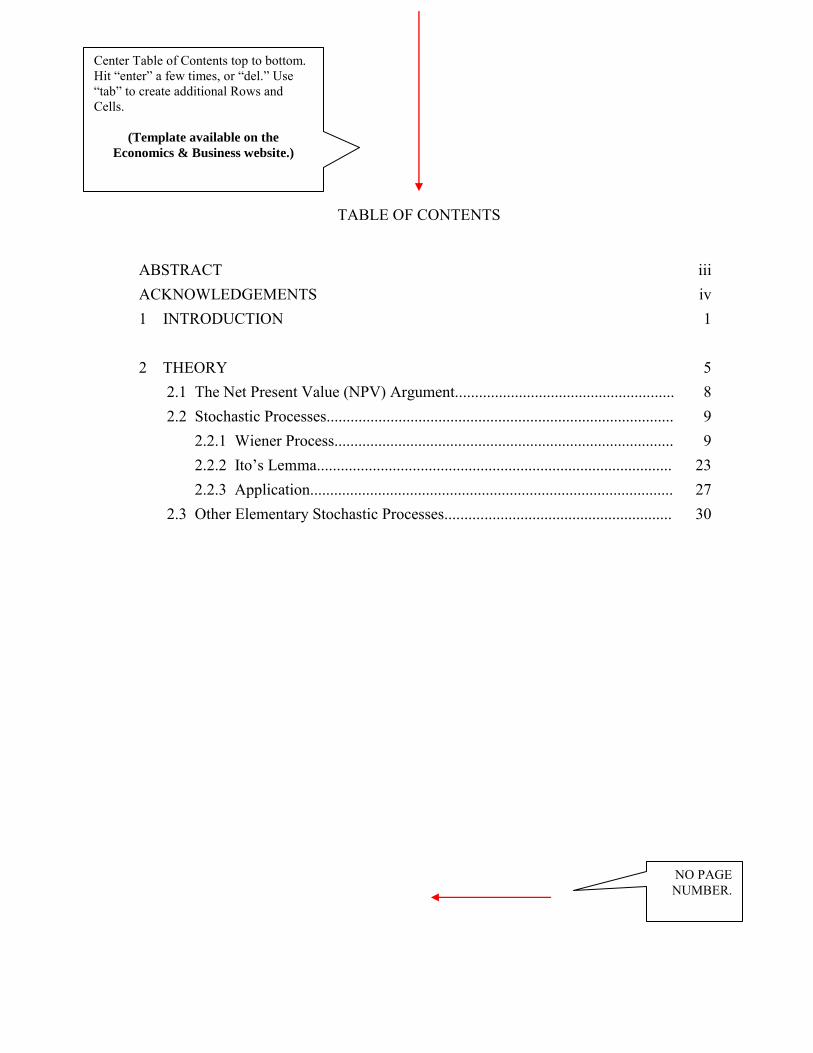
TABLE OF CONTENTS

ABSTRACT iii ACKNOWLEDGEMENTS iv 1 INTRODUCTION 1 2 THEORY 5 2.1 The Net Present Value (NPV) Argument....................................................... 8 2.2 Stochastic Processes....................................................................................... 9 2.2.1 Wiener Process..................................................................................... 9 2.2.2 Ito’s Lemma......................................................................................... 23 2.2.3 Application........................................................................................... 27 2.3 Other Elementary Stochastic Processes......................................................... 30

Center Table of Contents top to bottom. Hit “enter” a few times, or “del.” Use

“tab” to create additional Rows and

Cells.

(Template available on the

Economics & Business website.)

NO PAGE NUMBER.

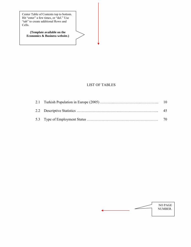
LIST OF TABLES

2.1 Turkish Population in Europe (2005) ………..………………….…………... 10

2.2 Descriptive Statistics …………………………….………………………….. 45

5.3 Type of Employment Status ………………………………………………… 70

Center Table of Contents top to bottom. Hit “enter” a few times, or “del.” Use

“tab” to create additional Rows and

Cells.

(Template available on the

Economics & Business website.)

NO PAGE NUMBER.

LIST OF FIGURES

3.1 Venture Capital Decision Process.……………………………………………. 26

3.2 Financing Decision……...…………………………………………………….. 31

3.3 Potential Investors…...………………………………………………………... 32

3.4 SBA Loan Process……..……………………………………………………… 34

3.5 Banks…..……………………………………………………………………… 35

3.6 Angel Investors……...………………………………………………………... 36

3.7 Venture Capital………..……………………………………………………… 37

Center top to bottom. Hit “enter” a few times, or “del.”

Use “tab” to create additional Rows

and Cells.

(Template available on the

Economics & Business website.)

NO PAGE NUMBER.

1

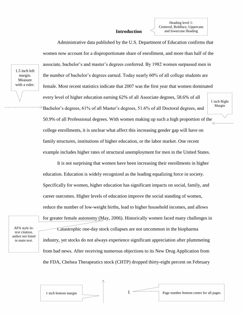
Introduction

Administrative data published by the U.S. Department of Education confirms that

women now account for a disproportionate share of enrollment, and more than half of the

associate, bachelor’s and master’s degrees conferred. By 1982 women surpassed men in

the number of bachelor’s degrees earned. Today nearly 60% of all college students are

female. Most recent statistics indicate that 2007 was the first year that women dominated

every level of higher education earning 62% of all Associate degrees, 58.6% of all

Bachelor’s degrees, 61% of all Master’s degrees, 51.6% of all Doctoral degrees, and

50.9% of all Professional degrees. With women making up such a high proportion of the

college enrollments, it is unclear what affect this increasing gender gap will have on

family structures, institutions of higher education, or the labor market. One recent

example includes higher rates of structural unemployment for men in the United States.

It is not surprising that women have been increasing their enrollments in higher

education. Education is widely recognized as the leading equalizing force in society.

Specifically for women, higher education has significant impacts on social, family, and

career outcomes. Higher levels of education improve the social standing of women,

reduce the number of low-weight births, lead to higher household incomes, and allows

for greater female autonomy (May, 2006). Historically women faced many challenges in

Catastrophic one-day stock collapses are not uncommon in the biopharma

industry, yet stocks do not always experience significant appreciation after plummeting

from bad news. After receiving numerous objections to its New Drug Application from

the FDA, Chelsea Therapeutics stock (CHTP) dropped thirty-eight percent on February

1.5 inch left

margin.

Measure

with a ruler.

1 inch Right

Margin

Page number bottom center for all pages

APA style in-

text citation,

author not listed

in main text.

1 inch bottom margin

Heading level 1:

Centered, Boldface, Uppercase

and lowercase Heading

2

13th, 2012 and saw its stock decline another sixty-seven percent from its February 13th

closing price over the next six months.

Figure 1.3. CHTP Stock Performance

Source: Stockcharts.com

Typical financial metrics used for valuation are irrelevant as most small

capitalization biopharmaceutical companies have little or no revenue. Investors place

huge bets for or against a company based on the perceived chance a drug will continue to

progress through the FDA process, which causes biopharma stocks to see the biggest

price gyrations in the market and makes them high-risk/high-reward investments. This

high volatility offers opportunities for enormous profits for well-timed trades. This begs

the question: Can a trader implement a strategy to achieve consistent abnormal profits

from taking a position after these large price drops? This paper begins to answer this

Figures should be

numbered to

include chapter

placement.

Title should

continue

immediately after

figure number in

upper and lower

case letters

If title is longer

than one line, the

subsequent lines

should be hanging

(indented).

Captions above

and below should be

centered.

Captions should

be a concise

explanation of

the figure and

explain any

symbols used in

the figure.

10

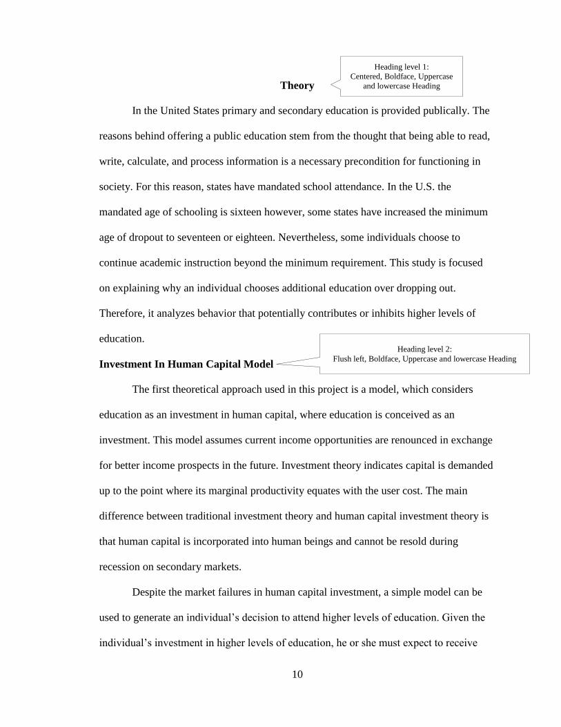
Theory

In the United States primary and secondary education is provided publically. The

reasons behind offering a public education stem from the thought that being able to read,

write, calculate, and process information is a necessary precondition for functioning in

society. For this reason, states have mandated school attendance. In the U.S. the

mandated age of schooling is sixteen however, some states have increased the minimum

age of dropout to seventeen or eighteen. Nevertheless, some individuals choose to

continue academic instruction beyond the minimum requirement. This study is focused

on explaining why an individual chooses additional education over dropping out.

Therefore, it analyzes behavior that potentially contributes or inhibits higher levels of

education.

Investment In Human Capital Model

The first theoretical approach used in this project is a model, which considers

education as an investment in human capital, where education is conceived as an

investment. This model assumes current income opportunities are renounced in exchange

for better income prospects in the future. Investment theory indicates capital is demanded

up to the point where its marginal productivity equates with the user cost. The main

difference between traditional investment theory and human capital investment theory is

that human capital is incorporated into human beings and cannot be resold during

recession on secondary markets.

Despite the market failures in human capital investment, a simple model can be

used to generate an individual’s decision to attend higher levels of education. Given the

individual’s investment in higher levels of education, he or she must expect to receive

Heading level 1:

Centered, Boldface, Uppercase

and lowercase Heading

Heading level 2:

Flush left, Boldface, Uppercase and lowercase Heading

11

higher wages after schooling. This higher wage is known as the college premium and is

used in simple wage equation models. If an individual experiences two life periods youth

(in period t) and adulthood in period (t+1) then the individual can devote a fraction of

his/her time to schooling in order to increase his/her stock of human capital Hit (Checchi,

2006: 18-19). Human capital is rewarded in the labor market by a higher wage rate βt.

Therefore, an individual’s incentive to accumulate higher levels of human capital is

shown by the increased future wage gains displayed in equation 3.1 (Checchi, 2006: 18-

19).

(3.1)

where Wij indicates the labor earnings of individual i in period j. The accumulation of

human capital requires time and does depreciate with time at a rate of δ which leaves

human capital accumulation to grow as given by equation 3.2.

(3.2)

(3.3)

therefore, human capital will accumulate based on the fraction of time spent on schooling

(S), on the individual’s innate ability (A), access to resources (libraries, family resources,

quality teachers) (E), and decreasing returns on time spent in education (H). In addition,

individuals face varying preferences for discounting the value of life-long earnings as

shown by equation 3.4 (Checchi, 2006).

Equation numbered on right margin

Additional equations

numbered along right

margin with chapter listed

first

APA

citation

for

author

not

listed in

main

text,

pages

known.

12

here, γt represents the direct cost of school attendance and ρ indicates the subjective rate

of intertemporal discount. If a perfect financial market existed, ρ would be replaced by

the market rate of interest.

Defining Access To Resources

As shown by the literature on human capital accumulation, access to resources is

a prominent indicator for an individual’s academic success. However, many variables

contribute to resource access, both at the individual’s elementary and secondary schools

as well as at home. This study classifies the following categories as access to resources

components of the game: family income, family academic resources, family household

characteristics, and secondary school resources.

Family Income. As shown by a vast amount of literature, family income is highly

correlated with an individual’s educational investment decision. Therefore, family

income is included in this study as part of an individual’s access to resources. Wealthier

families are more likely to invest in a child’s education and therefore, individual’s from

these families are likely to have access to higher quality schools such as a private

education, higher quality teachers as provided by higher income districts, and more

academic resources1.

In this study family income is taken at each survey and the categories are broken

down as follows: a high income family is noted by an income of $100,000 or greater, a

median income family is classified as an income of $20,000 to $100,000 and a low

1 The reasoning behind the idea that wealthier families place higher value on education, and are therefore

more willing to put greater resources towards their children’s education, stems from the idea that education

is a normal good, so as income increases, families will spend more on it. Additionally, as the “College

Pays” article highlights more highly educated families place greater emphasis on educating their children

(Baum, Ma, and Payae, 2010). Thus, having more wealth and greater levels of education in one generation

will lead to higher education levels in the following generation.

Heading Level 2

Flush left, Boldface, Uppercase and Lowercase Heading

Level

Heading 3:

Indented,

boldface,

lowercase

paragraph

heading

ending with

a period.

Footnotes are

for ancillary

comments only

13

income family is defined as a family with household income of $20,000 and below.

These values relate to high, medium, and low access to resources because a high income

family will have a child with high access to resources, a medium income family will have

a youth with medium access to resources, and a low income family corresponds with a

youth that has low access to resources. Family income as access to resources is closely

tied to the next sub-section: family academic resources.

Family academic resources. According to Teachman (1987), family background

resources are an important indicator of an individual’s academic success. A family that

provides academic resources is better able to prepare a youth for higher educational

attainment. Family academic resources include items like access to books at home, access

to newspapers at home, whether or not the parents provide a study space in the home

Level Heading

4:

Indented,

boldface,

italicized,

lowercase

paragraph

heading

ending with a

period.

APA in

text

citation

for

author

in main

text.

Table 4.2

Statistical Summary For Each Industry And The Entire Sample

Aerospace Mean Median Max Min Std. Dev. No. of

Obs.

Financial

Services

Mean Median Max Min Std.

Dev.

No.

of

Obs.

PRI 41.16 39.91 69.98 17.52 14.03 56 PRI 42.72 41.76 67.59 22.81 10.07 43

SI 0.22 0.15 2.30 -0.92 0.62 54 SI 0.22 0.16 2.00 -0.92 0.62 42

GPGR 11.31 11.71 76.14 -63.35 17.49 56 GPGR 16.49 11.37 247.38 -62.27 39.91 44

ROE 0.10 0.11 0.22 0.00 0.07 55 ROE 0.15 0.15 0.21 0.07 0.04 44

LIA 1.54 1.53 2.02 1.13 0.22 56 LIA 0.31 0.32 0.38 0.17 0.06 44

LEV 0.53 0.55 0.70 0.28 0.11 56 LEV 1.38 1.35 1.92 0.87 0.23 43

FCF 195.1

7

-22.62 2324.42 -362.91 562.45 56 FCF -

1367.29

-210.35 8347.56 -1449.79 3692.2

9

44

DIV 1.23 1.11 5.85 0.85 0.66 56 DIV 1.17 1.21 1.78 0.76 0.23 42

Healthcare Mean Median Max Min Std. Dev. No. of

Obs.

Healthcare Mean Median Max Min Std.

Dev.

No.

of

Obs.

PRI 47.57 47.87 75.16 28.06 10.89 56 PRI 43.33 43.04 68.87 24.61 9.89 56

SI 0.21 0.15 2.00 -0.92 0.60 54 SI 0.21 0.15 2.00 -0.92 0.60 54

GPGR 11.71 12.43 20.32 2.25 4.47 55 GPGR 11.43 11.82 109.85 -63.95 20.93 56

ROE 0.14 0.16 0.30 0.00 0.08 56 ROE 0.12 0.13 0.21 0.00 0.07 55

LIA 2.15 2.20 2.86 1.31 0.39 56 LIA 1.63 1.62 2.05 1.22 0.21 56

LEV 0.41 0.44 0.60 0.19 0.13 56 LEV 0.40 0.44 0.54 0.18 0.11 56

FCF 394.8

1

23.15 3307.59 -122.80 766.85 56 FCF -161.98 -28.61 2858.33 -3036.23 876.37 56

DIV 1.13 1.15 1.64 0.65 0.30 56 DIV 1.41 1.17 1.40 0.77 0.18 55

Source: 2011-2012 Thesis Guidelines and Illustrative Materials.

20

Man

ually

insert p

age n

um

bers

for lan

dscap

e pag

es

1.5 inch margin on top

22

Table 5.8

Weight Status, Body Dissatisfaction, and Weight Control Behaviors At Time 1 And

Suicidal Ideation At Time 2

Unadjusteda

Adjusted for

Demographic

Variablesb

Adjusted for

Demographic

Variables and Time

2 Depression

Variable OR 95% CI OR 95% CI OR 95% CI

Weight Status

Young men 0.97 [0.78, 1.21] 0.94 [0.75,1.19] 0.95 [0.74, 1.22]

Young women 1.06 [0.88, 1.26] 1.02 [0.85, 1.23] 1.02 [0.85, 1.23]

Body

Dissatisfaction

Young men 0.88 [0.50,1.54] 0.99 [0.56, 1.75] 0.67 [0.36, 1.24]

Young women 1.06 [0.77, 1.46] 1.02 [0.74, 1.42] 0.93 [0.93, 1.30]

UWCB

Young men 0.81 [0.54, 1.24] 0.77 [0.50, 1.19] 0.62 [0.39, 1.00]

Young women 0.89 [0.65, 1.21] 0.93 [0.68, 1.27] 0.82 [0.59, 1.13]

EWCB

Young men 1.36 [0.55, 3.36] 1.73 [0.69, 4.37] 1.66 [0.62-4.43]

Young women 1.98 1.34, 2.93] 2.00 [1.34, 2.99] 1.79 [1.19, 2.71]

Note. OR = odds ratio; CI = confidence interval; UWCB = unhealthy weight control behaviors; EWCB =

extreme weight control behaviors. Adapted from “Are Body Dissatisfaction, Eating Disturbance, and Body

Mass Index Predictors or Suicidal Behavior in Adolescents? A Longitudinal Study,” by S. Crow, M.E.

Eisenberg, M. Story, and D. Neumark-Sztainer, 2008, Journal of Consulting and Clinical Psychology, 76,

p 890. Copyright 2008 by the American Psychological Association. aFour weight-related variables entered simultaneously.

bAdjusted for race, socioeconomic status, and age

group.

Table number and table title: upper and

lower case letters. Title falls directly below

table number. If title is longer than one line

it should be flush with margin.

Tables may have three kinds of notes

placed below the table: general notes,

specific notes, and probability notes.

General notes should include explanations

that relate to the table as a whole including

the source of the table. Specific notes will

refer to particular columns or rows.

Wh

en a tab

le inclu

des p

oin

t estimates, fo

r exam

ple, m

eans,

correlatio

ns, o

r regressio

n slo

pes, it sh

ou

ld also

inclu

de

con

fiden

ce interv

als.

Tables should be aligned by decimal points.

Decked heads: heading that is stacked often to avoid

reputation or words in column headings

23

Table 5.15

Fixed Effects Estimates Of The Predictors Of Positive Parenting

Parameter Model 1 Model 2 Model 3 Model 4 Model 5

Intercept 12.51

(0.04)

12.23

(0.07)

12.23

(0.07)

12.23

(0.07)

12.64

(0.11)

Level 1 (Child Specific)

Age -0.49*

(0.02)

-0.48*

(0.02)

-0.48*

(0.02)

-0.48*

(0.02)

Age2 0.06*

(0.01)

0.06*

(0.01)

0.06*

(0.01)

0.06*

(0.01)

Negative Affectivity -0.56*

(0.08)

-0.53*

(0.08)

-0.57*

(0.09)

-0.57*

(0.09)

Girl 0.05

(0.05)

0.05

(0.05)

0.04

(0.05)

0.07

(0.05)

Not bio. mother -0.34

(0.26)

-0.28

(0.26)

-0.28

(0.26)

-0.30

(0.28)

Not bio. father -0.34*

(0.10)

-0.31*

(0.10)

-0.30*

(0.10)

-0.29

(0.15)

oldest sibling 0.38*

(0.07)

0.37*

(0.07)

0.37*

(0.07)

0.36*

(0.07)

middle sibling -0.36 *

(0.06)

-0.34*

(0.06)

-0.35*

(0.06)

-0.28*

(0.06)

Level 2 (family)

SES 0.18*

(0.06)

Marital dissatisfaction -0.43*

(0.14)

Family size -0.41*

(0.08)

Single Parent 0.09

(0.19)

All-girl sibship -0.20

(0.13)

Mixed gender sibship -0.25*

(0.10)

Note: Standard errors are in parentheses. Not bio. mother = not living with biological mother; not

bio. father = not living with biological father; SES = socioeconomic status. Adapted from “The

Role of the Shared Family Context in Differential Parenting,” by J.M. Jenkins, J. Rasbash, and

T.G. O’Connor, 2003, Developmental Psychology, 39, p. 104. Copyright 2003 by the American

Psychological Association.

*p<0.05.

Note should

include

significance

values

Stan

dard

errors o

r con

fiden

ce

interv

al sho

uld

be d

isplay

ed in

tables

with

mean

s, correlatio

ns, o

r

regressio

n slo

pes.