ysis and synthesis of concurrent - si2.epfl.chdemichel/graduates/theses/coelho.pdf · ws marcio,...
TRANSCRIPT

ANALYSIS AND SYNTHESIS OF CONCURRENT
DIGITAL SYSTEMS USING CONTROL-FLOW
EXPRESSIONS
a dissertation
submitted to the department of electrical engineering
and the committee on graduate studies
of stanford university
in partial fulfillment of the requirements
for the degree of
doctor of philosophy
Claudionor Jos�e Nunes Coelho Junior
February, 1996

c Copyright 1996
by
Claudionor Jos�e Nunes Coelho Junior
ii

I certify that I have read this thesis and that in my opin-
ion it is fully adequate, in scope and in quality, as a
dissertation for the degree of Doctor of Philosophy.
Giovanni De Micheli(Principal Adviser)
I certify that I have read this thesis and that in my opin-
ion it is fully adequate, in scope and in quality, as a
dissertation for the degree of Doctor of Philosophy.
David Dill(Associate Adviser)
I certify that I have read this thesis and that in my opin-
ion it is fully adequate, in scope and in quality, as a
dissertation for the degree of Doctor of Philosophy.
Bruce Wooley
Approved for the University Committee on Graduate
Studies:
iii

Abstract
We present in this thesis a modeling style and control synthesis technique for system-
level speci�cations that are better described as a set of concurrent descriptions, their
synchronizations and complex constraints. For these types of speci�cations, conven-
tional synthesis tools will not be able to enforce design constraints because these tools
are targeted to sequential components with simple design constraints.
In order to generate controllers satisfying the constraints of system-level speci�ca-
tions, we propose a synthesis tool called Thalia that considers the degrees of freedom
introduced by the concurrent models and by the system's environment.
The synthesis procedure will be subdivided into the following steps: We �rst
model the speci�cation in an algebraic formalism called control- ow expressions, that
considers most of the language constructs used to model systems reacting to their en-
vironment, i.e. sequential, alternative, concurrent, iterative, and exception handling
behaviors. Such constructs are found in languages such as C, Verilog HDL, VHDL,
Esterel and StateCharts.
Then, we convert this model and a suitable representation for the environment
into a �nite-state machine, where the system is analyzed, and design constraints such
as timing, resource and synchronization are incorporated.
In order to generate the control-units for the design, we present two scheduling
procedures. The �rst procedure, called static scheduling, attempts to �nd �xed sched-
ules for operations satisfying system-level constraints. The second procedure, called
iv

dynamic scheduling, attempts to synchronize concurrent parts of a circuit description
by dynamically selecting schedules according to a global view of the system.
v

Dedication
To Carla and Jean-Luc,
vi

Acknowledgments
I have many people to thank for this dissertation. First, in order to ful�ll one of Prof.
Giovanni De Micheli's last requests as an advisor, I shall be brief. So, instead of
saying all good things one usually says about advisors, I will just say that I consider
myself very fortunate to have him as my advisor and as a friend.
I would like to thank Prof. David Dill for all the help and support as a co-advisor.
I am also very thankful to him for allowing me to participate in the veri�cation
group meetings and discussions, where I learned a lot. Prof. Bruce Wooley has been
generous with his time by reading this dissertation. I would like to thank also Prof.
Teresa Meng and Prof. Gordon Kino for serving on my oral defense committee.
I have many thanks to the members of the CAD and veri�cation groups at Stan-
ford. Many good ideas and discussions followed the interaction with them, especially
with Luca Benini, Dave Filo, Rajesh Gupta, David Ku, Vincent Mooney, Polly Siegel,
Han Yang and Jerry Yang. I would like to thank Toshiyuki Sakamoto, who has been
working on the implementation of the Parnassus system. I have no words to thank
Lilian Betters for making my life at Stanford so much easier by dealing with the
university bureaucracy. Charlie Orgish and Thoi Nguyen have been very helpful in
keeping the machines working. I have also to thank the people with whom I shared
my o�ce in the trailers and at CIS (Dave Ofelt, Je� Kuskin, John Heinlein, and
Wingra Fang) for making a friendly o�ce environment.
Many friends I made at Stanford came from outside the research environment.
vii
Thanks to all of them, specially to the lunch group, Alexandre Santoro and Jo~ao
Comba, for making my lunch hours much more relaxing and enjoyable. Thanks
also to the several friends I have met here and who helped me throughout these
years: Antonio Todesco, Luis Portela, Ciro Noronha, Tyiomari, Angela Comba, Felipe
Guardiano, Alvaro Hernandez, Beto Cimini, Leda Beck, Ingrid and Luiz Franca.
Thanks also to Gilberto Mayor, Di�ogenes Silva, Berthier Ribeiro and Rodolfo Resende
for the friendship prior to my Stanford days.
I would like to thank my parents for believing in me and for all the support,
guidance and encouragement. Thanks also to the support given by Maria, Florinda
and by my in-laws Marcio, Domingos, Sirene and Carlos Vinicio.
Finally, I reserve a special gratitude to my beloved wife, Carla Nacif Coelho, for
her support, love, patience and encouragement during our stay at Stanford, and for
all the good moments we had here. Thanks to Jean-Luc, for bringing me the joy of
being a parent. To them I dedicate this thesis.
This research was sponsored by the scholarship 200212/90.7 provided CNPq/Brazil,
by a fellowship from Fujitsu Laboratories of America, and by ARPA, under grant No.
DABT 63-95-C-0049.
viii

Contents
Abstract iv
Dedication vi
Acknowledgments vii
1 Introduction 1
1.1 Overview of System-Level Synthesis : : : : : : : : : : : : : : : : : : : 3
1.2 Synthesis Tools used for System-Level Designs : : : : : : : : : : : : : 5
1.3 Issues in System-Level Synthesis : : : : : : : : : : : : : : : : : : : : : 8
1.3.1 Synchronization Synthesis : : : : : : : : : : : : : : : : : : : : 9
1.3.2 Scheduling under Complex Interface Constraints : : : : : : : : 14
1.4 Objectives and Contributions : : : : : : : : : : : : : : : : : : : : : : 16
1.5 Thesis Outline : : : : : : : : : : : : : : : : : : : : : : : : : : : : : : : 18
2 Modeling of Concurrent Synchronous Systems 20
2.1 Abstraction Model : : : : : : : : : : : : : : : : : : : : : : : : : : : : 21
2.2 Algebra of Control-Flow Expressions : : : : : : : : : : : : : : : : : : 25
2.3 Axioms of Control-Flow Expressions : : : : : : : : : : : : : : : : : : 31
2.4 Extended Control-Flow Expressions : : : : : : : : : : : : : : : : : : : 34
2.4.1 Exception Handling : : : : : : : : : : : : : : : : : : : : : : : : 36
ix

2.4.2 Basic Blocks : : : : : : : : : : : : : : : : : : : : : : : : : : : : 42
2.4.3 Register Variables : : : : : : : : : : : : : : : : : : : : : : : : : 43
2.4.4 De�nition of Extended Control-Flow Expressions : : : : : : : 48
2.5 Comparison of CFEs with Existing Formalisms : : : : : : : : : : : : 50
2.6 Summary : : : : : : : : : : : : : : : : : : : : : : : : : : : : : : : : : 56
3 Modeling the Environment 58
3.1 Quanti�cation of the Design Space : : : : : : : : : : : : : : : : : : : 59
3.2 Constraint Speci�cation : : : : : : : : : : : : : : : : : : : : : : : : : 63
3.2.1 Dynamically Satis�able Constraints : : : : : : : : : : : : : : : 66
3.2.2 Statically Satis�able Constraints : : : : : : : : : : : : : : : : 71
3.3 Summary : : : : : : : : : : : : : : : : : : : : : : : : : : : : : : : : : 76
4 Analysis of Concurrent Systems 78
4.0 Notation : : : : : : : : : : : : : : : : : : : : : : : : : : : : : : : : : : 79
4.1 Control-Flow Finite State Machines : : : : : : : : : : : : : : : : : : : 79
4.1.1 Derivatives of Control-Flow Expressions : : : : : : : : : : : : 81
4.1.2 Derivatives in Extended Control-Flow Expressions : : : : : : : 84
4.1.3 Control-Flow Expression Su�xes : : : : : : : : : : : : : : : : 91
4.1.4 Revisiting Exception Handling : : : : : : : : : : : : : : : : : : 94
4.2 Constructing the Finite State Representation : : : : : : : : : : : : : : 95
4.2.1 Satis�ability of Design Constraints : : : : : : : : : : : : : : : 99
4.3 Representation of CFFSM as a Transition Relation : : : : : : : : : : 100
4.3.1 Characteristic Functions and Transition Relation : : : : : : : 100
4.3.2 Representation of the CFFSM Using the Transition Relation : 101
4.3.3 Computing Reachable States and Valid Transitions : : : : : : 107
4.4 Summary : : : : : : : : : : : : : : : : : : : : : : : : : : : : : : : : : 109
x

5 Synthesis of Control-Units 110
5.1 Obtaining Control-Units from the CFFSM : : : : : : : : : : : : : : : 111
5.2 Scheduling Operations in Basic Blocks : : : : : : : : : : : : : : : : : 114
5.3 Static Scheduling Operations in CFFSMs : : : : : : : : : : : : : : : : 118
5.3.1 Extracting Constraints from the CFFSM : : : : : : : : : : : : 119
5.3.2 Exact Scheduling for Basic Blocks : : : : : : : : : : : : : : : : 132
5.4 Dynamic Scheduling Operations in CFFSMs : : : : : : : : : : : : : : 139
5.4.1 Selecting the Cost Function : : : : : : : : : : : : : : : : : : : 143
5.4.2 Derivation of Control-Unit : : : : : : : : : : : : : : : : : : : : 146
5.5 Comparison with Other Scheduling Methods : : : : : : : : : : : : : : 149
5.6 Summary : : : : : : : : : : : : : : : : : : : : : : : : : : : : : : : : : 151
6 Experimental Results 153
6.1 The E�ects of Encoding on the Synthesis Procedure : : : : : : : : : 155
6.2 Protocol Conversion : : : : : : : : : : : : : : : : : : : : : : : : : : : 156
6.3 Control-Unit for Xmit frame : : : : : : : : : : : : : : : : : : : : : : : 161
6.4 FIFO Controller : : : : : : : : : : : : : : : : : : : : : : : : : : : : : : 164
7 Conclusions and Future Work 168
7.1 Summary : : : : : : : : : : : : : : : : : : : : : : : : : : : : : : : : : 168
7.2 Future Work : : : : : : : : : : : : : : : : : : : : : : : : : : : : : : : : 170
Bibliography 172
A Algebra of Synchronous Processes 182
B Binary Decision Diagrams 185
xi

List of Tables
1 Link between Verilog HDL constructs and control- ow expressions : : 30
2 Axioms of control- ow expressions : : : : : : : : : : : : : : : : : : : : 33
3 One-hot encoding for decision variables : : : : : : : : : : : : : : : : : 155
4 Binary encoding for decision variables : : : : : : : : : : : : : : : : : : 156
5 Gray encoding for decision variables : : : : : : : : : : : : : : : : : : : 157
6 PCI/SDRAM protocol conversion example : : : : : : : : : : : : : : : 160
7 Results for the synthesis of xmit frame : : : : : : : : : : : : : : : : : 164
8 Results for the synthesis of xmit frame with dynamic variable ordering
of BDDs : : : : : : : : : : : : : : : : : : : : : : : : : : : : : : : : : : 164
9 Axioms for ASP : : : : : : : : : : : : : : : : : : : : : : : : : : : : : : 184
xii

List of Figures
1 System-level tasks : : : : : : : : : : : : : : : : : : : : : : : : : : : : : 6
2 Ethernet controller block diagram : : : : : : : : : : : : : : : : : : : : 9
3 Abstracted behaviors for DMArcvd, DMAxmit and enqueue : : : : : 12
4 System architecture : : : : : : : : : : : : : : : : : : : : : : : : : : : : 14
5 Writing cycles for synchronous DRAM (a) and for synchronous FIFO
(b) : : : : : : : : : : : : : : : : : : : : : : : : : : : : : : : : : : : : : 15
6 Thesis outline : : : : : : : : : : : : : : : : : : : : : : : : : : : : : : : 18
7 Partitioning of speci�cation into control- ow/data ow : : : : : : : : : 24
8 Greatest-common divisor example : : : : : : : : : : : : : : : : : : : : 35
9 Hierarchical View of a CFE : : : : : : : : : : : : : : : : : : : : : : : 38
10 Conversion between C constructs and ECFE disable constructs : : : : 40
11 Exception handling in Verilog HDL : : : : : : : : : : : : : : : : : : : 41
12 Data ow for Di�erential Equation Fragment : : : : : : : : : : : : : : 43
13 Program-State Machine Speci�cation : : : : : : : : : : : : : : : : : : 44
14 (a) Speci�cation and (b) Reduced dependency graph : : : : : : : : : 45
15 (a) Data ow graphs for program-state machine and (b) reduced de-
pendency graph : : : : : : : : : : : : : : : : : : : : : : : : : : : : : : 48
16 Static and dynamic decision variables : : : : : : : : : : : : : : : : : : 59
17 Minimum (a) and maximum (b) execution times for the operations of
the di�erential equation CDFG : : : : : : : : : : : : : : : : : : : : : 61
xiii

18 Process P and its Environment : : : : : : : : : : : : : : : : : : : : : 65
19 Path-activated constraint : : : : : : : : : : : : : : : : : : : : : : : : : 73
20 Exception handling in Verilog HDL : : : : : : : : : : : : : : : : : : : 75
21 Mealy machine for control- ow expression (a � b � c)! : : : : : : : : : : 80
22 Finite-state representation for synchronization synthesis problem : : : 96
23 Algorithm to construct �nite-state representation : : : : : : : : : : : 98
24 Finite-state representation observing synchronization constraints : : : 99
25 Encoding for Basic Block of Di�erential Equation : : : : : : : : : : : 102
26 Encoding for Sequential/Parallel Blocks : : : : : : : : : : : : : : : : : 103
27 Exception Handling in CFFSMs : : : : : : : : : : : : : : : : : : : : : 106
28 Algorithm to Compute Transition Relation of a CFE : : : : : : : : : 107
29 Algorithm to Compute Reachable States of a CFFSM : : : : : : : : : 108
30 Methodology for synthesizing control-units : : : : : : : : : : : : : : : 112
31 (a) Graphical representation of CFE p and (b) CFFSM for p : : : : : 123
32 Finite-State Machine Representing the Path-Activated Constraint : : 124
33 Algorithm to Compute a Minimum Path-Activated Constraint in a
CFFSM : : : : : : : : : : : : : : : : : : : : : : : : : : : : : : : : : : 127
34 Algorithm to Compute a Maximum Path-Activated Constraint in a
CFFSM : : : : : : : : : : : : : : : : : : : : : : : : : : : : : : : : : : 128
35 Path-Activated Constraint FSM for min (2; [a1; c]) : : : : : : : : : : : 129
36 Algorithm to Compute Solve : : : : : : : : : : : : : : : : : : : : : : : 137
37 Implementation for CFFSM : : : : : : : : : : : : : : : : : : : : : : : 138
38 Path cost selection in CFFSM : : : : : : : : : : : : : : : : : : : : : : 146
39 Implementations for control- ow expression p3 = ((x : 0)�:a)! : : : : : 148
40 Block diagram of Parnassus Synthesis System : : : : : : : : : : : : : 154
41 Protocol conversion for PCI bus computer : : : : : : : : : : : : : : : 158
42 PCI write cycle : : : : : : : : : : : : : : : : : : : : : : : : : : : : : : 159
xiv

43 PCI read cycle : : : : : : : : : : : : : : : : : : : : : : : : : : : : : : 159
44 SDRAM read and write cycles : : : : : : : : : : : : : : : : : : : : : : 160
45 Program state machine for process xmit frame : : : : : : : : : : : : : 161
46 Implementation of program state machine with exception handling : : 163
47 Datapath for FIFO controller : : : : : : : : : : : : : : : : : : : : : : 165
48 High-level view of FIFO controller : : : : : : : : : : : : : : : : : : : : 166
49 Binary Decision Diagram for function x1x2 : : : : : : : : : : : : : : : 186
50 BDD representing the constraint 4x1 + 5x2 � 8 : : : : : : : : : : : : 187
xv

Chapter 1
Introduction
The use of synthesis tools in synchronous digital designs at the logic and higher levels
has gained large acceptance in industry and academia. Three of the reasons for its
acceptance are the increasing complexity of the circuits, the need for reducing time
to market and the requirement to design circuits correctly and optimally. In order to
meet these requirements of today's marketplace, designers have to rely on the ability
to specify their designs at higher levels of abstraction. In particular, designers depend
upon models that describe the speci�cation at a level higher than logic level and RTL
level [Mic94].
Above the logic level of abstraction, circuit designs have been described at high-
level and system-level. We denote by high-level abstraction the modeling style based
on the representation of a circuit design by blocks of operations and their dependen-
cies. High-level abstraction has been used e�ectively for representing designs in digital
signal processing applications [VRB+93]. However, when representing designs that
are better speci�ed as a set of concurrent and interacting components, this abstraction
level will not be able to capture the synchronization introduced by the components
executing concurrently.
1

2 CHAPTER 1. INTRODUCTION
We call system-level abstraction a modeling style based on the description of con-
current and interacting modules and system-level synthesis the corresponding task
of deriving a logic-level description from such a model. Concurrency allows design-
ers to reduce the complexity by partitioning the circuit into smaller components.
Communication guarantees that these concurrent parts will cooperate to determine
the correct circuit behavior. For example, communication processors, such as the
MAGIC chip [KOH+94] and an ethernet coprocessor [HLS], are representative de-
signs of systems speci�ed at this level of abstraction. These descriptions consist of
several protocol handlers that execute concurrently and interact through data trans-
fers and synchronization.
Traditionally, system-level designs have been synthesized by high-level synthesis
tools [MPC90], where synthesis is performed by partitioning the circuit description
into sequential blocks containing operations, which are scheduled over a discrete time
and bound to components [KM92]. This technique is called single process synthesis
in [WTHM92], since it ignores concurrency and communication in the beginning, thus
focusing only on the sequential parts of the design. After the synthesis is performed
on each concurrent component, they are combined at the lower levels, i.e. at RTL or
logic-level. Note that at this level the results are already suboptimal and harder to
optimize.
Single process synthesis imposes severe restrictions on system-level designs. First,
since only one sequential component is synthesized at a time, the synthesis tool cannot
consider the degrees of freedom available in other concurrent parts of the design.
Second, the interface uses a model that does not consider communication. As a
result, intricate relations between a model and its environment cannot be enforced
during synthesis. Finally, single process synthesis targets area or delay optimization
of each sequential block, which may not yield an optimal design since the design
contains concurrent and interacting components. For example, the minimization of

1.1. OVERVIEW OF SYSTEM-LEVEL SYNTHESIS 3
the execution time in a concurrent speci�cation requires the minimization of delays
over execution paths.
This dissertation focuses on modeling, analysis and synthesis of concurrent and
communicating systems. In particular:
� We present an algebraic model for concurrent and communicating systems that
gives a formal interpretation for system-level descriptions, such that these sys-
tems can be abstracted, analyzed and synthesized.
� We present a technique for scheduling operations subject to complex interface
constraints and synchronizations.
� We present a technique for synchronizing the concurrent parts of the design by
dynamically scheduling operations or blocks of operations.
1.1 Overview of System-Level Synthesis
System-level design contains sub-components showing sequential, alternative, concur-
rent, repetition and exception handling behaviors [GVNG94]. We assume that the de-
sign is originally speci�ed by a description language supporting these behaviors, such
as VHDL [LSU89], Verilog HDL [TM91], HardwareC [KD90], StateCharts [DH86],
Esterel [BS91].
Synthesis of system-level designs di�ers from standard high-level synthesis [DKMT90,
CBH+91, WTHM92, KLMM95] because the emphasis of the tool is placed on con-
current models and their interactions. In addition, implementation of system-level de-
signs are often not con�ned to a single chip or a hardware implementation alone [Gup93].
As a result, the steps of partitioning, scheduling, synchronization, interface synthe-
sis, and datapath generation in system-level synthesis will focus in the generation of

4 CHAPTER 1. INTRODUCTION
controllers subject to constraints crossing the concurrent models of the speci�cation
and di�erent implementation paradigms.
In system-level synthesis, partitioning involves the selection of clusters of opera-
tions and models that should be synthesized together [DGL92, TWL95] and clusters
that should be synthesized separately. A good partition will be obtained by clustering
parts of the speci�cation that are tightly coupled and share the same critical resources
of the design. This will allow the tools used at the later stages of the design to better
optimize the cluster.
Another important task of system-level synthesis is scheduling. Scheduling denotes
the assignment of operations over discrete time slots. Although high-level synthesis
also considered scheduling as a synthesis task, we emphasize here the di�erences
between scheduling in high-level synthesis and scheduling in system-level synthesis.
In high-level synthesis, the main emphasis is put into the scheduling of operations
within a basic block. Optimality of a design in high-level synthesis is usually given in
terms of the optimality of the execution time in basic blocks or the cost of resources
in basic blocks, such as the number of multipliers, adders or multiplexors. In system-
level synthesis, on the other hand, we have to consider the interactions that cross
basic block boundaries as well. When the system is partitioned in clusters some
of the interactions of the system are converted into environment constraints, which
should guide the tool in �nding feasible and optimal implementation. Whenever
these environmental constraints cross implementation paradigms (such as hardware
and software), appropriate synchronization must be added as well. In addition to this,
the optimality criteria in system-level synthesis shifts from basic blocks to whole parts
of the design. For example, in a cache controller, the speci�cation can be divided into
a hit and miss case, both of which can share some parts of the speci�cation. Since
the hit case is going to be executed more often than the miss case, the primary
optimization goal should be the minimization of the execution time of the hit path,

1.2. SYNTHESIS TOOLS USED FOR SYSTEM-LEVEL DESIGNS 5
and using the minimization of the execution time of the miss case as a secondary
goal.
Synchronization and interface synthesis refers to the generation of protocol con-
verters for some parts of the design. At the system-level of the speci�cation, the user
may have not committed to a protocol for the communication of the events across
concurrent parts of the design, or the speci�cation of the protocol may already exist in
the form of libraries. In synchronization synthesis, the tool produces protocols for the
communication among di�erent parts of the speci�cation, and generates converters
between protocol libraries and the speci�cation, according to the design constraints.
Finally, in datapath generation we obtain datapaths for the operations and their
dependencies in the speci�cation. During datapath generation, the tool selects com-
ponents for an implementation, binds the components to operations, and binds the
variables of the speci�cation into registers.
Figure 1 gives an example of the tasks involved in the synthesis of system-level
designs. From the speci�cation of a concurrent system, a system-level tool �rst par-
titions the description and generates a set of crossing these partitions, then the tool
schedules the operations over a discrete time according to the environmental con-
straints, synthesizes the synchronization skeletons and protocols for the di�erent parts
of the speci�cation, and generates datapaths for the operations and variables.
1.2 Synthesis Tools used for System-Level Designs
Many systems implemented by Application Speci�c Integrated Circuits (ASICs) are
control-dominated applications [Keu89]. In such applications, high-level synthesis
techniques have been used previously to synthesize control-units for system-level de-
signs.

6 CHAPTER 1. INTRODUCTION
Sender Receiver
alwaysbegin data = receive(ch); @posedge clk;end
alwaysbegin send(ch,data); data <= data + 1;end
data
+
1
data
data
1 send
data <= data + 1 @posedge clk
receive
Specification
Partitioning
Synchronization Synth.
data
data
1
Scheduling
Data−path Generation
Figure 1: System-level tasks
The Olympus Synthesis System [DKMT90] targets control-dominated ASIC de-
signs. Starting from the high-level language HardwareC, the system performs the
high-level synthesis tasks of scheduling operations over discrete times, binding oper-
ations to components and variables to registers. One of the unique features of the
Olympus Synthesis System is that it allows the user to specify synchronization and
data transfers using high-level message passing communication constructs. In this
system, send and receive operations are used to generate synchronizations and to
transfer data across concurrent models. Although HardwareC allows the system to
be speci�ed using concurrent and communicating modules, the synthesis technique
applied in these modules considers only one module at a time, preventing the synthe-
sis from utilizing the degrees of freedom from the other modules during the synthesis
of a single module.

1.2. SYNTHESIS TOOLS USED FOR SYSTEM-LEVEL DESIGNS 7
The HIS System [CBH+91] was developed at IBM to synthesize mixed data ow
intensive/control- ow intensive speci�cations. The system being synthesized was �rst
partitioned into its control- ow/data ow components, for which a control unit and
datapath were generated, respectively [Cam91]. In path-based scheduling, operations
in a path can be scheduled into a single discrete time as long as it does not have
any con icts with the other operations scheduled in the same discrete time. Because
scheduling is performed on a path-basis, this algorithm is able to schedule operations
across sequential, alternative and repetitive control- ow structures.
The Princeton University Behavioral Synthesis System [WTHM92] (PUBSS) and
the Synopsys Behavioral Compiler [KLMM95] were conceived using ideas similar to
those of the HIS system. Both systems allow control- ow with arbitrary sequential,
alternative and repetitive behaviors. In addition to that, PUBSS is able to consider
more aggressive timing constraints than the previous systems described in this section,
called path activated constraints. PUBSS is also able to handle the tightly coupled
parts of the design by merging them together during synthesis. Nevertheless, it is not
able to cross parallel composition barriers, which may exist in Verilog or StateChart
descriptions.
The Clairvoyant system [Sea94] was designed for the speci�cation and control
generation of control-dominated applications using a grammar-based speci�cation
language. The system is speci�ed using a grammar languages supporting sequential,
alternative and parallel composition, loops, synchronization and exception handling.
Since the Clairvoyant system does not allow the incorporation of any design con-
straints, the synthesis technique is limited to a syntax-directed translation from the
grammar speci�cation to the control-unit, and thus all timing information must be
already present and scheduled during the speci�cation of the design.
We will describe in this thesis a tool called Thalia 1 for system-level synthesis
1The muse of comedy
8 CHAPTER 1. INTRODUCTION
that will be unique because it will be able to handle several of the design issues
regarding system-level designs, some of which were mentioned in this section. We
will consider speci�cations containing sequential, alternative, parallel compositions,
loops and exception handling mechanisms. Such constructs are present in Verilog,
StateCharts, and VHDL. We will not limit the speci�cations to contain concurrency
only at the highest levels of the speci�cation, as it is the case in IBM Synthesis
System, PUBSS and Synopsys Behavioral Compiler. We will be also consider general
forms of design constraints, which will help us to model the environment, and exible
objective functions, which will help us to better cast our design goal.
In the next section, we will present some design problems that will help us to
better understand the issues in system-level synthesis.
1.3 Issues in System-Level Synthesis
This section presents examples of designs that either cannot be synthesized or are
synthesized sub-optimally by typical high-level synthesis tools. We show intuitively
that valid and optimal implementations can be obtained only if synchronization,
dynamic scheduling and scheduling with complex timing and resource constraints are
considered during the design space exploration.
One of the major problems of using current synthesis tools to implement system-
level designs is that the tool must consider how the environment a�ects the model
being synthesized. Since the speci�cation of the environment in which the circuit is
going to execute is generally a formidable task, the user must have a better control
over the synthesis tool in order obtain optimal results. With Thalia, the user can
specify complex environment constraints and exible cost functions.
In the next three examples, we motivate the reader about the need for tools that
can handle concurrent and communicating systems.

1.3. ISSUES IN SYSTEM-LEVEL SYNTHESIS 9
1.3.1 Synchronization Synthesis
In this example, we show how we can synchronize multiple processes sharing the
same critical resource. We will see that this synchronization can be synthesized only
if we consider the degrees of freedom among the di�erent processes that share the
critical resource. We are going to see that the model being synthesized will have to
dynamically recon�gure itself in order to allow other models to use the same resource
at di�erent times. In this example, in order to obtain a feasible solution, we have
to specify a constraint that spans across concurrent models, i.e., the critical resource
should not be used by more than one model at a time.
HostCPU
Memory
System Bus
DMA−RCVD
RCVD−FRAME RCVD−BUFFER RCVD−BIT
DMA−XMIT XMIT−FRAME XMIT−BIT
ENQUEUE EXEC−UNIT
RXE
RXD
TXD
TXE
CRS
CDT
Receive Unit
Transmit Unit
Execute Unit
Ethernet Coprocessor
Figure 2: Ethernet controller block diagram
The block diagram of an ethernet coprocessor is shown in Figure 2. This coproces-
sor contains three units: an execution unit, a reception unit and a transmission unit.
These three units are modeled by thirteen concurrent processes, with three processes
accessing the bus: DMAxmit , DMArcvd , and enqueue. The problem we want to

10 CHAPTER 1. INTRODUCTION
solve is the synthesis of the synchronization among the three processes such that any
bus access for the three processes is free of con icts. Note that the di�culty in solving
this problem comes from the transfers that are non-deterministic over time, i.e., we do
not know a priori when each process accesses the bus, since this operation is control
dependent. Also, the transfers of di�erent processes are uncorrelated, i.e. knowing
that one process accesses the bus at a speci�c time does not imply the transfers in
other processes are known.
Related Work in Synchronization Synthesis
The problem of synchronizing critical resources across concurrent models has been
solved for the simpli�ed assumption that the models are data ows executing at the
same rate [HP92]. Note that in the problem described here, however, we do not
know when each bus access will take place, since we may have arbitrary control- ow
speci�cations that will make the bus accesses to be dependent on the environment
and to execute at di�erent rates. Thus, the approach described in [HP92] cannot be
used for the bus accesses of the ethernet coprocessor described here.
Filo et al. [FKJM93] addressed the problem by rescheduling transfers inside a
single loop or conditional to reduce the number of synchronizations among processes.
This method is restrictive because all transfers that are optimized must be enclosed
in the same loop or conditional, and only the synchronizations due to the transfers
are considered during the simpli�cation. A synchronization is eliminated if its exe-
cution is guarded by a previous synchronization. As we are going to show later, our
formalism allows processes to be speci�ed by their control- ow with an abstraction on
the data ow parts, and thus will subsume the solutions found by the two approaches
previously discussed. Also, our formalism achieves the simpli�cation of synchroniza-
tion that crosses loops and conditionals, and we do not restrict this simpli�cation to
only transfers present in single loops or conditional branches, as in [FKJM93].

1.3. ISSUES IN SYSTEM-LEVEL SYNTHESIS 11
In [CE81], the system was speci�ed by a set of �nite state machines and a set
of properties speci�ed using CTL (Computation Tree Logic) formulae. These for-
mulae characterized the desired behavior of the system in terms of safety (\nothing
bad ever happens") and liveness (\something good eventually happens") properties.
Each machine of the system was considered to execute asynchronously with respect to
the other machines, and a product machine was obtained by combining the machines
of all speci�cations. A synchronizer was extracted from the product machine such
that this sub-machine satis�ed the set of CTL formulae. A similar method was also
reported in [Wol82], but using linear time temporal logic formulae for specifying the
temporal properties of the system. This model considered concurrency of the speci-
�cations as an interleaving of executions, as opposed to the model we will de�ne in
the next chapter, which will consider true concurrency. As a result, the synchronizers
generated by these procedures will be subject to much stricter constraints than they
will experience.
Zhu et al. [ZJ94, ZJ93a] used timing expressions to capture synchronizations of
models. A timing expression is an expression containing timing relations between a
set of signals, which are expressed using traces of executions. In his descriptions,
the system is speci�ed by a set of timing expressions and the synchronization is
speci�ed by a set of constraints a system has to satisfy. These constraints have been
solved by [Zhu92] using an algorithm that returns a set of timing expressions for the
synchronizers. Timing expressions can be useful for determining relationships among
signals in a timing diagram, as shown in [ZJ94], when every signal of a timing diagram
is represented by a timing expression and the synchronization constraints represents
how these signals interact. However, timing expressions will not be able to capture
the intricate relations that are present in higher-level descriptions.

12 CHAPTER 1. INTRODUCTION
Synchronization Synthesis for the Ethernet Coprocessor
Let us �rst consider an abstraction of the original speci�cation that captures only the
bus accesses. Furthermore, in order to be able to discuss this problem throughout
this paper, we will assume a set of reduced behaviors for DMArcvd, DMAxmit and
enqueue such that the resulting behavior is small enough that can be easily under-
stood. Figure 3 presents the behaviors we assume for these descriptions in this paper,
in a pseudo-Verilog code. In this �gure, the constructs that do not belong to the
language, such as write bus, are represented in typewriter style; reserved words of
Verilog are represented in bold; and other legal syntactic constructs are represented in
italics. The signal transmission ready is assumed to be set by the environment sur-
rounding the three processes, and free bus represents the waiting period for process
enqueue.
module DMArcvd;
always
begin
write bus;
data = receive(from xmit frame);
end
endmodule
module DMAxmit;
always
begin
initialize variables
wait (transmission ready);
read bus;
end
endmodule
module enqueue;
always
begin
wait (free bus);
read bus;
end
endmodule
Figure 3: Abstracted behaviors for DMArcvd, DMAxmit and enqueue
The processes shown in the �gure are control-dominated speci�cations where the
ow of control is modi�ed by some set of wait statements. In this example, also, note
that the priority of enqueue should be the smallest one, since the execution of the
bus access in this process may be delayed. On the other hand, if the bus accesses of
the other processes are delayed, the controller will not be able to deliver data at the
interface at the proper rate.
We assume that processes DMArcvd and DMAxmit have already been synthesized,

1.3. ISSUES IN SYSTEM-LEVEL SYNTHESIS 13
and their cycle-based behaviors are presented in the �gure. We are interested in
obtaining a control-unit for process enqueue such that it will not have con icting bus
accesses with neither DMArcvd nor DMAxmit. Note that in order to synthesize the
waiting period for enqueue we must know when the other process will access the bus.
Therefore, enqueue must have a global view of the bus accesses of the other processes
in order to decide when it can access the bus.
If we assume that every operation takes one clock cycle, an implementation for the
synchronization mechanism of the bus should establish a temporal relation between
enqueue and the two other processes DMAxmit and DMArcvd. This temporal relation
should include any data-dependent operation of the two other processes, such as the
conditional transmission ready, and it should also consider when the other processes
access the bus. A possible solution to this problem would be:
module enqueue;
always
begin
@ ( posedge clock);
if (transmission ready)
begin
@ ( posedge clock);
end
else begin
read bus;
end
end
endmodule
In this implementation, we have to wait the �rst cycle because DMArcvd is ac-
cessing the bus in the �rst cycle. During the second cycle, enqueue will be able to
access the bus only if DMAxmit is not accessing it. In the following cycle, however,
DMArcvd will be accessing the bus again, and enqueue will have to wait for another
cycle. We will show later how this controller could be obtained automatically for the
process enqueue.

14 CHAPTER 1. INTRODUCTION
1.3.2 Scheduling under Complex Interface Constraints
PROGRAM
uP
MEMORY
ASIC
send(addr,data)
FIFO
Figure 4: System architecture
In this example, we show how we can specialize a design by incorporating dynamic
scheduling constraints from an interface. Splitting the interface speci�cation from
the design speci�cation was addressed in [NG95, KM92, NT86, Bor88]. One of the
main advantages of abstracting interface implementation details at the higher levels
of abstraction is that more degrees of freedom can be explored during synthesis.
In such techniques, the transfers among processes are abstracted in terms of com-
munication operations (such as a send operation). During synthesis, the best protocol
and communication medium is selected to implement a particular transfer. The selec-
tion and synthesis of the protocol interface will impose complex scheduling constraints
to the design, as we will see below.
Consider a system that has an ASIC and an embedded processor, such as the one
given in Figure 4. Assume the ASIC communicates with the microprocessor either
through a synchronous memory or through a synchronous FIFO. For example, this
structure has been used in hardware-software codesign [GJM92, GJM94]. In this
system, the transfers to the memory and to the FIFO are determined at run-time
by the proper selection of the address. The interface timing is also determined at
run-time, since the timing speci�cations for these two components are di�erent, as

1.3. ISSUES IN SYSTEM-LEVEL SYNTHESIS 15
Cas
Ras
CLK
Data
Addr
We Data
WCLK
WEN
(A) (B)
Figure 5: Writing cycles for synchronous DRAM (a) and for synchronous FIFO (b)
given in Figure 5. In essence, a data transfer may take either one or three cycles to
complete. Thus, the timing constraint speci�cation should also re ect the mismatch
between the timing of the components.
The speci�cation of interface constraints has been used in the past by Nestor [NT86],
Ku [KM92] and Borriello [Bor88]. They used min/max scheduling constraints to an-
notate the design speci�cation. The use of these constraints, however, is limited to
static constraints. In the example presented above, the speci�cation of the interface
requires the design to contain implementation details, which is not desirable for the
reasons given previously.
Assuming that the address selection for the memory module is called s, the con-
straint that we need to specify is a three-cycle operation or a one-cycle operation,
depending on s. Thus, the interface can no longer be speci�ed in terms of �xed min-
imum/maximum delay between operations, since the execution time of the operation
is dependent on the address selection. In order to synthesize the protocol for the send
operation given above, we must consider a dynamic schedule for this operation.
This can be achieved by using the alternative composition in the constraint spec-
i�cation. For example, one possible representation for this constraint could be:

16 CHAPTER 1. INTRODUCTION
synchronize with \send" operation
if (s)
delay for \send" is 3 cycles
else
delay for \send" is 1 cycle
We will show that using the algebra of control- ow expressions, we can represent
this constraint as the following compact representation:
s : Ras � 0 � fCas,datag+ s : data
where Ras is an abstraction to the RAS cycle of the RAM, Cas is an abstraction of
the CAS cycle of the RAM, 0 is a one-cycle delay operation, data is an abstraction of
the data transfer, and s means that s is false.
During the synthesis procedure, the send operation is bound to an implementation
that observes this constraint. In this case, the implementation is exactly the control
that waits either one or three cycles, depending on s.
In this example, the two di�erent communications mechanisms assume di�erent
possible behaviors for the environment. Depending on how the environment requires
data, one mode should be highlighted over the other for some transfer by the proper
selection of an objective function.
1.4 Objectives and Contributions
In this thesis, we present a formal model to analyze system-level designs targeted
to control- ow intensive applications, and a methodology to synthesize the control-
units for the concurrent parts of the design. Because many applications found in
Application Speci�c Integrated Circuits are control-dominated applications [Keu89],
we will address the following issues regarding control- ow dominated system-level
designs.

1.4. OBJECTIVES AND CONTRIBUTIONS 17
� Modeling. We will present a model to represent the control- ow of concurrent
systems that includes most of the control- ow constructs present in speci�cation
languages, such as sequential, parallel and alternative compositions and loops.
In addition to that, our model will support exception handling mechanisms
which are present in languages such as Verilog HDL, Esterel and StateCharts.
We will also allow systems to be speci�ed with programming languages, such
as C. Finally, we will include in our model some of the variables of the speci�-
cations, since in some cases these variables can give a better understanding of
the control- ow behavior in such systems.
� Constraints. We will show how we can incorporate complex constraints of
the design. The constraints of the design will not be limited to the constraints
usually speci�ed in high-level synthesis tools, but we will also allow the model's
environment to be speci�ed and to synchronize with the model being synthe-
sized.
� Analysis. We will present techniques for analysis of the speci�cation and its
environment in a �nite-state machine representation, and we will show how we
can e�ciently represent this �nite-state machine. In this �nite-state machine,
we will be able to detect when no control-unit can be obtained for a speci�cation
when the speci�cation is composed with its environment.
� Synthesis. We will present two techniques for solving the scheduling and
synchronization synthesis problems. In the �rst technique, we will schedule
operations statically over time to satisfy complex interface constraints. In the
second technique, we will dynamically schedule the interacting parts of the
speci�cation in order to synchronize them. These schedules and the speci�cation
can be used to obtain a control-unit for the circuit description that optimizes a
design goal, while satisfying the environment constraints.

18 CHAPTER 1. INTRODUCTION
1.5 Thesis Outline
The outline of this thesis (which is also the outline of the tool we developed) can be
seen in Figure 6.
Integer Linear Programming
Control−Unit Implementation
Control−Flow Expressions
Control−Flow Finite State Machine
Specification Constraints
Chapter 4 (Analysis)
Chapter 2 (Modeling)
Chapter 2 (Modeling) Chapter 3 (Environment Constraints)
Chapter 5 (Synthesis)
Figure 6: Thesis outline
After the introduction and motivation described in this chapter, Chapter 2 de-
scribes our model for concurrent control-dominated systems, called control- ow ex-
pressions. There, we present the algebra of control- ow expressions, and we show how
this algebra can be used to model the control- ow aspects of a speci�cation. Then,
we present extensions to the algebra of control- ow expressions that will allow us to
consider more realistic system-level designs, by incorporating some variables into the
1.5. THESIS OUTLINE 19
control- ow model, and by allowing the speci�cation to contain exception handling
mechanisms.
Since our model assumes that the system will be interacting with other models
and with the environment, in Chapter 3 we will present techniques to incorporate
design constraints into control- ow expressions. These constraints will include timing,
resource and synchronization constraints.
Chapter 4 presents a method to analyze the system consisting of control- ow
expressions by converting the system into a speci�cation automaton that contains
all degrees of freedom of the system being synthesized. We will also show how to
represent this speci�cation automaton in terms of a transition relation, and how
to e�ciently encode the di�erent constructs of the control- ow expressions into the
transition relation.
Chapter 5 describes two synthesis methods for scheduling operations and syn-
chronizing parts of the description. Both of these algorithms are implemented as
restrictions on the behavior of the speci�cation automaton obtained in the previous
chapter.
Chapter 6 presents some design examples and how they could be solved using
the formulation presented in this thesis. Finally, in Chapter 7, we will present some
concluding remarks and some ideas for future research.

Chapter 2
Modeling of Concurrent
Synchronous Systems
We will be focusing in this chapter on a model for control-dominated system-level
descriptions. Since system-level descriptions are usually speci�ed as sets of concurrent
components interacting among themselves and with the environment, an optimal
controller can be obtained only if we understand the underlying behavior of the system
to be synthesized, and its relation to the environment.
We model the system in terms of control- ow and data ow for each concurrent
component. We will �rst attempt to restrict the control- ow to the control- ow
constructs of conventional structured languages, and we will restrict the data ow
model to the variables, and their corresponding operations. This abstraction model
is presented in Section 2.1.
In Section 2.2, we present the algebra of control- ow expressions, which is an alge-
braic model for representing the control- ow of system-level designs, while abstracting
away the data ow details. In Section 2.3, the axioms of control- ow expressions will
be introduced. These axioms form the basis for the analysis technique we will develop
in the next chapter.
20

2.1. ABSTRACTION MODEL 21
In order to better analyze the control- ow of system-level designs, it will be shown
in Section 2.4 that variables and operations may play a fundamental role in de�ning
the control- ow behavior, and we will show which parts of the data ow must be
considered during analysis and synthesis of control- ow dominated speci�cations.
In addition to that, in order to capture basic blocks of traditional programming
languages and hardware description languages, we will introduce blocks in control- ow
expressions. Finally, exception handling mechanisms will also be added to control-
ow expressions in order to capture the rupture of structured control- ow in the
designs, usually due to the occurrence of exceptions that is common to most hardware
description languages.
In Section 2.5, we compare extended control- ow expressions with existing for-
malisms that capture the control- ow of concurrent systems.
2.1 Abstraction Model
We consider in this thesis system-level designs that will be synthesized as synchronous
digital circuits running under the same clock. In the synthesis of these designs, we
need to represent the interactions among the concurrent parts, which can be best
modeled at the control- ow level.
We assume in our computation model that the speci�cation will be partitioned
in terms of a control- ow and a data ow, as described in [DGL92, Mic94, ZJ93b].
In this model, variables, their operations and operands are placed in the data ow,
and the constructs determining the ow of control of the speci�cation language are
placed in the control- ow. I/O operations between a process and the process external
environment will be placed in the data ow. We formalize this model below.

22 CHAPTER 2. MODELING OF CONCURRENT SYNCHRONOUS SYSTEMS
Data ow
We de�ne a data ow by its structure, without considering the meaning of the opera-
tions in the speci�cation, similarly to the de�nitions of [ZJ93b]. Let V = fv1; . . . ; vng
be a set of variables, and let v be a generic element of V. We assume that constant
values are speci�ed by variables whose names are represented by the constant value.
Let F be a set of functions whose typical elements are f and fi.
De�nition 2.1 An operation is de�ned as v f(v1; . . . ; vn), i.e., variable v is as-
signed the result of function f , when the function's parameters are set to the variables
v1; . . . ; vn.
We call the set of operations O. A data ow can be de�ned as a set of operations
and a partial order among them. It can be depicted as a directed acyclic graph
in which vertices are operations and edges correspond to dependencies among the
operations. Each edge is annotated with the variable that creates the dependency.
Control-Flow
In a hardware speci�cation, as well as in a software program, the sequencing of the op-
erations is determined by control- ow constructs, such as procedure calls, branching
and iteration. In particular, descriptions can be made hierarchical by using procedure
calls, which encapsulate portions of the behavior. Such a hierarchy may be abstracted
as a directed acyclic graph, whose root corresponds to the overall system, whose inter-
nal vertices correspond to sequential, parallel, alternative and iterative compositions,
and whose leaves are either operations, or groups of operations and data ow models.
Di�erent models [DGL92, Mic94, GVNG94] have been proposed to represent
branching and iteration. In this thesis, we represent branching and iteration hier-
archically, with their bodies being modeled as procedure calls, i.e. at a lower level

2.1. ABSTRACTION MODEL 23
in the representation hierarchy. Such calls are invoked conditionally according to the
value of the branching or iterative clauses.
Note that in the control- ow and data ow models de�ned above, the execution
of the control- ow is data-dependent, and because the data ow is conditionally exe-
cuted, according to the control- ow, the data ow is control-dependent. Since at this
level of abstraction, the execution time for the operations is not known yet, in order
to consider the communication between the data ow and the control- ow we model
the interface by instantaneous events. The control- ow generates output events to
the data ow that sensitize the execution of operations in the data ow. The data ow
generates input events to the control- ow that trigger the di�erent execution paths.
Example 2.1.1. In Figure 7, we show the representation of a speci�cation
in terms of its control- ow and data ow graphs.
The vertices loop and alt in the control- ow graph represent iterative and al-
ternative behavior, respectively.
We labeled each operation in the data ows by events a1; . . . ; a6. Such events are
generated by the control- ow and determine when the corresponding operations
will execute. Event a1, for example, triggers the execution of the negation of
dx. These events determine the dependency of the data ow with respect to the
control- ow. Each data ow also contains two vertices, source and sink that do
not correspond to any operation in the speci�cation. They mark the beginning
and end of execution of the data ow, respectively.
The data ow of Figure 7 generates input events c1 and c2 that trigger the
execution of the loop and the execution of the alternative path, respectively.
These events determine the dependency of the control- ow in terms of the
data ow.
The reader should note that the control- ow does not make any assumptions
on the possible values of its input events over time. In this example, we assume
that entering the loop (when event c1 is generated) and exiting the loop are
equally probable, for example. 2
We model a concurrent system by looking at the interface between the data ow
and the control- ow, i.e. at the events the control- ow generates and consumes. As a
result, we need to abstract data ow details from our model. We abstract the details

24 CHAPTER 2. MODELING OF CONCURRENT SYNCHRONOUS SYSTEMS
output [...] dx,dy;... while (a > 0) begin dx = !dx; a = a − 1; dy = a; if (dy == 1) dx = 0; end
source
dx
!
sink
dx
−
a
a
=
==
dy
c2
1
1
source
sink
=dx
0
source
sink
>a 0
c1
alt
loop
c2
c1
(a1)
(a2)
(a3)
(a4)
(a5)
(a6)
Control−Flow Dataflow
Figure 7: Partitioning of speci�cation into control- ow/data ow
from the data ow by considering three mappings at the interface between the data ow
and control- ow: a timing mapping, a binding mapping and a synchronization map-
ping. The timing mapping associates an execution time with every computation or
component. The binding mapping associates the possible functions of a computation
with their possible implementations. Finally, the synchronization mapping speci�es
how the concurrent parts interact. The control- ow and the three mappings de�ned

2.2. ALGEBRA OF CONTROL-FLOW EXPRESSIONS 25
in this paragraph provide the means by which we can analyze the validity of the spec-
i�cation with respect to design constraints, as well as the means to generate possible
implementations.
2.2 Algebra of Control-Flow Expressions
The algebra of control- ow expressions (CFEs) is de�ned by the abstraction of the
speci�cation in terms of the sensitization of paths in the data ow, and by the compo-
sitions that are used among these operations. As presented in the previous section,
we view the communication between the data ow and control- ow as an event gener-
ation/consumption process. More formally, we call the output events generated from
the control- ow actions (from some alphabet A). We assume that each action will
execute in one-unit of time (or cycle). If an operation executes in multiple cycles,
they will be handled by a composition of single-cycle actions.
Example 2.2.2. The C fragment presented below corresponds to a part of
a di�erential equation solver found in [Mic94].
xl = x + dx;
ul = u - (3 * x * u * dx) - (3 * y * dx);
yl = y + u * dx;
c = x1 < a;
During the compilation of this description, the expressions are broken into a
set of prede�ned operations including addition, multiplication, subtraction and
comparison.
m1 = 3 * x; /* m1 */
m2 = u * dx; /* m2 */
m3 = m1 * m2; /* m3 */
m4 = 3 * y; /* m4 */
m5 = m4 * dx; /* m5 */
m6 = u * dx; /* m6 */
a1 = x + dx; /* a1 */
yl = y + m6; /* a2 */

26 CHAPTER 2. MODELING OF CONCURRENT SYNCHRONOUS SYSTEMS
c = a1 < a; /* lt */
s1 = u - m3; /* s1 */
u1 = s1 - m5; /* s2 */
If we assume that each operation described above executes in one cycle, we can
represent the operations above by actions m1; m2; m3; m4; m5; m6; a1; a2; lt; s1
and s2, according to the comments to the right of the code. 2
We represent the input events of a control- ow by conditionals, which are symbols
from an alphabet C. The conditionals in a control- ow expression will enable di�erent
blocks of the speci�cation to execute. Guards will be de�ned as the set of the Boolean
formulas over the set of conditionals.
De�nition 2.2 A guard is a Boolean formula on the alphabet of conditionals. We
will use G to denote the set of guards over conditionals.
We assume that each guard and conditional is evaluated in zero time. At the
end of this section, we compare the assumptions on the execution time of actions,
conditionals and guards with the synchrony hypothesis.
Example 2.2.3. In the speci�cation if (x � y) x = y * z, a conditional
c abstracts the binary relational computation x � y. If at some instant of
time, the guard c is true, x = y * z is executed. If at some instant of time,
the guard :c is true, the else branch (which is null in this case) is executed. 2
Using control- ow expressions, we model systems by a set of operations, dependen-
cies, concurrency and synchronization. We encapsulate sub-behaviors of this system
in terms of processes, which are represented by control- ow expressions and corre-
spond to an HDL model. In our representation, each process is a mapping from labels
of the alphabet F to control- ow expressions.
We de�ne the set � as the alphabet of actions, conditionals and processes � =
A [ C [ F .

2.2. ALGEBRA OF CONTROL-FLOW EXPRESSIONS 27
The compositions that are de�ned in the algebra of control- ow expressions are
the compositions supported by existing HDLs which were captured by the control- ow
model described earlier. Verilog HDL, for example, supports sequential composition,
alternative composition, loops, parallelismand unconditional repetition. The same set
of compositions is also supported in VHDL and HardwareC, and thus is supported by
control- ow expressions. Since alternative compositions and loops in these languages
are guarded, their corresponding compositions in CFEs will also be guarded.
The setO = fsequential(�); alternative(+); guard(:); loop(�); in�nite(!); parallel(jj)g
is de�ned to be the valid compositions of control- ow expressions. The formal de�-
nition of the algebra of control- ow expressions is presented below:
De�nition 2.3 Let (�;O; �; �) be the algebra of control- ow expressions where:
� is an alphabet that is subdivided into the alphabet of actions, conditionals and
processes;
O is the set of composition operators that de�ne sequential, alternative, guard,
loop, in�nite and parallel behavior;
� is the identity operator for alternative composition;
� is the identity operator for sequential composition.
We can now de�ne the control- ow expressions recursively.
De�nition 2.4 Control- ow expressions are:
� Actions a 2 A.
� Processes p 2 P.
� � and �.

28 CHAPTER 2. MODELING OF CONCURRENT SYNCHRONOUS SYSTEMS
� If p1; . . . ; pn are control- ow expressions, and c1; . . . ; cn are guards, then the
following expressions are control- ow expressions.
{ The sequential composition, represented by p1 � . . . � pn
{ The parallel composition, represented by p1k . . . kpn
{ The alternative composition, represented by c1 : p1 + . . . + cn : pn
{ Iteration, represented by (c1 : p1)�
{ Unconditional repetition, represented by p!1.
Nothing else is a control- ow expression.
Informally, we de�ne the behavior of the compositional operators of CFEs as
follows: the sequential composition of p1, . . . , pn means that pi+1 is executed only
after pi is executed, for i 2 f1; . . . ; n � 1g. The parallel composition of p1, . . . ,
pn means that all pi's begins execution at the same time for i 2 f1; . . . ; ng. The
alternative composition of p1, . . . , pn guarded by c1, . . . , cn, respectively, means that
pi only begins execution if the corresponding ci is true. Iterative composition means
that p1 begins execution while the guard c1 is true. The in�nite composition means
that p1 begins execution in�nitely many times upon reset.
We introduced in the previous de�nition the symbol � that is called here deadlock1.
The symbol � is de�ned as ��= false : p, where p is any control- ow expression. The
deadlock symbol is an identity for alternative composition. This means that the
branch of the alternative composition represented by the deadlock is never reachable.
Later we show that these branches can in fact be removed.
1Deadlock was the name given to � in process algebras. In synthesis, � denotes code that is
unreachable due to synchronization. Since its properties are the same as the properties for deadlock
in process algebras, we used the latter name, for the sake of uniformity.
2.2. ALGEBRA OF CONTROL-FLOW EXPRESSIONS 29
We also introduced the symbol �, which is called here the null computation. The
null computation symbol is de�ned as a computation that takes zero time. For ex-
ample, this symbol can be used to denote an empty branch of a conditional. This
symbol behaves as the identity symbol for sequential composition.
Note that in our de�nition of the syntax of CFEs, every loop and every alternative
branch is guarded by \:", which makes the di�erent branches of alternative and loops
distinct. We also assume that only one alternative branch will be taken at any given
time. This restricts the speci�cation of loop bodies and alternative branches to only
accept deterministic choices with respect to the guards.
For the sake of simplicity, we restrict the sets of behaviors de�nable in control- ow
expressions in the following way: it should always be possible to obtain a control-
ow expression without any process variables, i.e. we should be able to eliminate
recursion from a control- ow expression by substituting process variables by their
respective CFE, with the recursion on a process variable being replaced by iterative
or unconditional repetition. In this thesis, whenever we refer to a CFE p, we are
referring to the CFE without recursion de�ned by the process variable p.
Although this assumption seems to constrain the representation model using
CFEs, in practice this will not impose problems because CFEs captures exactly the
control- ow constructs of structured languages such as Verilog HDL and VHDL.With
respect to C, we use a subset of C that does not allow a function to be de�ned re-
cursively in order to avoid the possibility of having a CFE with process variables
for which no CFE without process variables can be obtained. Later in this chapter
we will enrich control- ow expressions by allowing CFEs to break the conventional
ow of control, as in the case of breaks, continues and returns of the C programming
language, or as in the case of disables of the Verilog HDL.
In control- ow expressions, we consider a special action called 0, which corre-
sponds to a no-operation or abstraction of the computation. Action 0 executes in one

30 CHAPTER 2. MODELING OF CONCURRENT SYNCHRONOUS SYSTEMS
Composition HL Representation CF Expression
Sequential begin p; q end p:q
Parallel fork p; q join pjjq
Alternative
if (c)
p ;
else
q ;
c : p+ c : q
Loop
while (c)
p ; (c : p)�
wait (!c)
p ; (c : 0)�:p
In�nitealways
p ;p!
Table 1: Link between Verilog HDL constructs and control- ow expressions
unit-delay (just as any other action), but it corresponds either to an unobservable
operation of a process with no side e�ects or to a unit-delay between two computa-
tions.
Whenever possible, we will relate the HDL constructs to control- ow expressions,
instead of using the control- ow/data ow model described earlier for sake of simplic-
ity.
The semantics of the major control- ow constructs in HDL are related to control-
ow expressions in the table in the Table 1, where p and q are processes (p; q 2
F) and c is a conditional (c 2 C). In this �gure, we relate CFEs to the control-
ow structure of Verilog HDL [TM91]. In this thesis, we assume that guards (:)
have precedence over all other composition operators; loops and in�nite composition
(�; !) have precedence over the remaining compositions; sequential composition (�)
has precedence over alternative and parallel composition; alternative composition (+)
has precedence over the parallel composition. In addition to that, we use parentheses

2.3. AXIOMS OF CONTROL-FLOW EXPRESSIONS 31
to overrule this precedence and for ease of understanding. Although it is not necessary,
we will at times replace parentheses by square brackets for clarity.
We will use the following shorthand notation for control- ow expressions. The
control- ow expression pn will denote n instances of p composed sequentially (p � . . . � p| {z }n
),
which corresponds, for example, to a counting loop that repeats n times in some HDL.
The control- ow expression (x : p)<n will denote a control- ow expression in which
at most n� 1 repetitions of p may occur. This CFE is equivalent to (x : p+x : �)n�1.
In our original speci�cation, we assumed that every action in A takes a unit-time
delay in CFEs, and that every guard takes zero time delay. Then, we could possibly
design a system where after choosing a particular branch of an alternative composition
(e.g., after choosing c is true in c : p+ c : q) and executing the �rst action of process
p, the execution of this action would make c true and thus also enable the execution
of q. In order to avoid this erroneous behavior, we adopt a weaker version of the
synchrony hypothesis [BS91].
Assumption 2.1 Let p be a process and c be a guard that guards the execution of p
(de�ned as c : p). Any action of p is assumed to execute after c has been evaluated
to true. In order words, c : p can be viewed as (c : �) � p. First, the conditional
is evaluated to true, then the process p that is guarded by c is executed, and other
assignments to c will possibly a�ect future choices only.
2.3 Axioms of Control-Flow Expressions
The algebra of control- ow expressions inherits its formalism from a subset of pro-
cess algebras [Bae90] that is suitable for describing synchronous reactive systems,
called the algebra of regular synchronous processes. We further extend this algebra
by specifying Boolean variables as guards of processes. We refer the reader to Ap-
pendix A for a de�nition of the algebra of synchronous processes similar to the one

32 CHAPTER 2. MODELING OF CONCURRENT SYNCHRONOUS SYSTEMS
found in [Bae90]. The following proposition relates control- ow expressions to the
algebras of synchronous processes.
Proposition 2.1 CFEs are a subset of regular synchronous process algebras.
In this section, we present the axioms for the algebra of control- ow expressions
by extending the axioms de�nitions of process algebras to handle actions and condi-
tionals. These axioms provide the theoretical background that will be used to build
the �nite-state machine representation for control- ow expressions in Section 4.1.
In Table 2, we present the axioms of control- ow expressions, where a and b are
multisets of actions, p; q; r 2 F (processes) and c1; c2; c3 2 G (guards).
The alternative composition has � as its identity component. It is commutative,
and associates to the right or left. The sequential composition has � as its identity
component. It associates to both the right and left, and it is only distributive to the
left with respect to the alternative composition. This implies that p � (c1 : r+c2 : s) 6=
c1 : p � r + c2 : p � s. The intuitive meaning for p � (c1 : r + c2 : s) being di�erent from
c1 : p � r + c2 : p � s is that we abstracted away the computation of p, c1 and c2, and
thus we cannot answer the question on whether an action in p a�ects the choice of c1
or c2, or if the environment needs some value from p for making a decision on whether
c1 or c2 should be true. If we assumed this transformation were valid, we could make
the decision for all branches of the speci�cation upon start by propagating the guards
towards the beginning.
On the other hand, if we assumed that p � (c1 : r + c2 : s) were equivalent to
p � c1 : r + p � c2 : s, we would be in fact assuming that system were non-causal (its
current choices depending on the future value of conditionals) and in this case we
could also have propagated all those decisions to the initial start time of the system
modeled by the CFE.

2.3. AXIOMS OF CONTROL-FLOW EXPRESSIONS 33
c1 : p+ c2 : q = c2 : q + c1 : p (+ is commutative)
(c1 : p+ c2 : q) + c3 : r = c1 : p+ (c2 : q + c3 : r) (+ is associative)
= c1 : p+ c2 : q + c3 : r
(c1 : p+ c2 : q) � r = c1 : p � r + c2 : q � r (� distributes to the left with +)
(p � q) � r = p � (q � r) (� is associative)
= p � q � r
c1 : p+ c1 : p = c1 : p (+ is idempotent)
1 : p = p
0 : p = �
c1 : p+ � = c1 : p (� is the identity element for +)
� � p = � (� is the zero element for �)
p � � = p (� is the identity element for �)
� � p = p
c1 : c2 : p = (c1 ^ c2) : p
ajjb = (a [ b) if a [ b synchronize
ajjb = � if a [ b does not synchronize
ajjb = bjja
ajj0 = a
ajj� = a
a � pjjb � q = (ajjb) � (pjjq)
a � pjjb = (ajjb) � p
(c1 : p+ c2 : q)jjr = c1 : (pjjr) + c2 : (qjjr)
Table 2: Axioms of control- ow expressions
The parallel composition assumes synchronous execution semantics, also known
as maximal parallelism semantics. In these execution semantics, if two processes are
executed in parallel, then one action of each process is executed atomically at the
same time. We represent the actions that execute together by multisets of actions.
For example, if multiset a de�nes fa1; . . . ; ang, where each ai 2 A, actions a1; . . . ; an
are executed at the same time. The set consisting of multisets of actions is represented
here by the symbolMA. If two multisets a = fa1; . . . ; ang and b = fb1; . . . ; bmg are
composed in parallel, the resulting multiset fa1; . . . ; an; b1; . . . ; bmg is represented by
a [ b. We sometimes abuse our notation for multisets and use ai for faig if it can be

34 CHAPTER 2. MODELING OF CONCURRENT SYNCHRONOUS SYSTEMS
inferred by the context that ai represents the multiset faig.
In the de�nition of the axioms of CFEs, we showed that the result of the parallel
composition of two multisets a and b is dependent on some synchronization between
a and b. Although a formal de�nition of synchronization will be presented in the next
chapter, we will give an informal de�nition that will allow the reader to understand
its meaning.
Processes synchronize in control- ow expressions in two ways. The �rst way is
by de�ning multisets of actions that always have to execute at the same time, or by
de�ning multisets of actions that should never execute at the same time. The second
method of synchronization is achieved by de�ning guards that generate a deadlock
when conjoined.
Loops and in�nite computations can be de�ned by control- ow expressions with
process variables. The loop composition (c : p)� is equivalent to recursive process
q = c : p � q + c : �, where p is a process variable. The in�nite composition p! is
equivalent to the recursive process q = p � q. Their axioms can be determined by
applying those equations into axioms of the original algebra.
Example 2.3.4. We provide here an example of the representation of
Verilog HDL constructs in control- ow expressions. The speci�cation shown in
Figure 8 consists of an algorithmic representation of a greatest common divisor.
Its control- ow expression is represented by process p, where the labels on the
right correspond to the actions being executed or the conditionals on alternative
compositions.
p = [(r : 0)� � b � (c1 : (c2 : (c3 : c)� � d)� � e+ c1 : �)]
!
2
2.4 Extended Control-Flow Expressions
In the previous section, we presented the basic constructs for control- ow expres-
sions capturing most of the control- ow constructs of structured languages. In this

2.4. EXTENDED CONTROL-FLOW EXPRESSIONS 35
module GCD(Xin; Y in; ready; result);
input [7 : 0] Xin; Y in;
input ready;
output [7 : 0] result;
reg [7 : 0] result; x; y;
always
begin
wait (ready) // conditional r
fx; yg = fXin; Y ing; // action b
if (x! = 0 && y! = 0) // conditional c1
begin
while (y! = 0) // conditional c2
begin
while (x >= y) // conditional c3
x = x� y ; // action c
fx; yg = fy; xg ; // action d
end
result = x ; // action e
end
end
endmodule
Figure 8: Greatest-common divisor example
section we revise the control- ow expression model, and we extend it to incorporate
exception handling mechanisms encountered in hardware description languages. Ex-
tended control- ow expressions (ECFEs) will be formally de�ned in Section 2.4.4,
after having presented their motivation and usage.
One interesting observation about the control- ow expression model we devel-
oped in the previous sections is that it captures the control- ow of series-parallel 2
representation of systems. In imperative programming languages, however, blocks of
operations and their dependencies usually cannot be represented e�ciently using this
series-parallel representation, and as a result, in order to e�ciently consider them in
our model we will add basic blocks to CFEs.
2We denote by a series-parallel system the representation of a system in terms of mixture of
sequential and parallel compositions

36 CHAPTER 2. MODELING OF CONCURRENT SYNCHRONOUS SYSTEMS
Finally, as shown in Section 2.1, we modeled the communication between the
control- ow and data ow through events. Sometimes, this communication can be
reduced if some of the variables mapped into the data ow are considered during the
control- ow analysis, such as variables representing states of program-state machines
or counters. We will present in this section the general theory under which such de-
viations from the traditional approach to control/data ow partitioning can be made.
As opposed to the axioms presented in the previous sections, the properties for
the extended control- ow expressions will be presented only in Chapter 4, since the
system's properties will be better understood at the �nite-state machine level, which
is de�ned in Chapter 4.
2.4.1 Exception Handling
We assume the system-level design was speci�ed by a structured language such as
C, Verilog HDL or VHDL, with limited forms of disruption of the control- ow. In
particular, all compositions de�ned for CFEs have single exit points. In this section,
we enrich CFEs to allow systems to be described using multiple exit points from
the control- ow. This extension will add to the e�ciency in the representation of
more complex control- ow structures, such as exception handling mechanisms that
are present in reactive systems.
Examples of the disruption in the control- ow of structured languages can be
found in both C and Verilog HDL. In C speci�cations, returns, breaks and continues
are used to exit the procedure (as in the case of return) or the inner most loop (as in
the case of break or continue). In Verilog HDL, multiple-exits from the control- ow
corresponds to a limited form of the disable statement.
The exception handling mechanism added in this section is called disable (for its
similarities with the disable statement in Verilog) that allows the control- ow to be
disrupted at any point in the hierarchy. As it was shown in the control- ow model

2.4. EXTENDED CONTROL-FLOW EXPRESSIONS 37
presented earlier, the control- ow of a speci�cation can be viewed as a hierarchical
composition of other control- ows. Similarly, the corresponding CFE can be seen
as a hierarchical composition of other CFEs. In particular, the uplink of a control-
ow expression represents a snapshot of the hierarchy with respect to a control- ow
expression.
De�nition 2.5 Let p and q be control- ow expressions. An n � uplink relation
between p and q can be de�ned recursively as follows.
� Control- ow expression q is a 0-uplink of p if q = p.
� If qi is a n-uplink of p, then q is a n + 1-uplink of p in the following CFEs.
{ q = q0 � . . . � qi � . . . � qn;
{ q = c0 : q0 + . . . + ci : qi + . . . + cn : qn;
{ q = q0jj . . . jjqijj . . . jjqn;
{ q = q!i ;
{ q = (ci : qi)�.
The de�nition above de�nes q as an uplink of a CFE p by counting how many
compositions of control- ow expressions are necessary to obtain CFE p containing q.
This de�nition is better explained by the example below.
Example 2.4.5. The control- ow expression for the GCD algorithm of
Example 2.3.4 is presented below, and its directed acyclic graph representation
is presented in Figure 9, according to the composition rules for CFEs. In this
graph, nodes represent control- ow expression composition rules, with actions
and � being the terminal vertices. The edge (p; q) represents the relation the
control- ow p can be obtained by a composition of q.
p = [(r : 0)� � b � (c1 : (c2 : (c3 : c)� � d)� � e+ c1 : �)]
!
The following uplinks are de�ned for action c in CFE p.

38 CHAPTER 2. MODELING OF CONCURRENT SYNCHRONOUS SYSTEMS
.
*
0
b +
.
* e
.
* d
c
ω
ε
Figure 9: Hierarchical View of a CFE
� c is a 0-uplink of c in p.
� (c3 : c)� is a 1-uplink of c in p.
� (c3 : c)� � d is a 2-uplink of c in p.
� (c2 : (c3 : c)� � d)� is a 3-uplink of c in p.
� (c2 : (c3 : c)� � d)� � e is a 4-uplink of c in p.
� (c1 : (c2 : (c3 : c)� � d)� � e+ c1 : �) is a 5-uplink of c in p.
� (r : 0)� � b � (c1 : (c2 : (c3 : c)� � d)� � e + c1 : �) is a 6-uplink of c in p.
� p is a 7-uplink of c in p.
2
The uplink of a control- ow expression is used to determine where in the hierarchy
the control- ow should continue the execution after executing the disable operation.

2.4. EXTENDED CONTROL-FLOW EXPRESSIONS 39
De�nition 2.6 �(n; p) is an extended control- ow expression that takes zero time
and returns the control- ow to the ECFE following the n-uplink of �(n; p) in p.
This de�nition can be seen as the execution of the extended control- ow expression
following the n-uplink of �, when the ECFE represented by the n-uplink of � is replaced
by an �. The de�nition of � above introduces a technicality into the axioms of control-
ow expressions. Recall that ((p1 � p2) � p3) � (p1 � p2 � p3). In order for this axiom to
be valid when we consider ECFE �, we have to compute the uplink with respect to
the original speci�cation p, and not with respect an ECFE p0 equivalent to p. Thus,
if p is a n-uplink of �(m; p) in p, and even though p � p0, we still keep the expression
�(m; p) in p0.
We will refer to ECFE � as the disable construct in this thesis. The de�nition
above for the disable construct allows us to represent C's breaks, continues and re-
turns, as seen in the following propositions.
Proposition 2.2 A break command in C can be converted into a disable operation
in extended control- ow expressions, where n is the least uplink enclosing a loop, an
in�nite computation or an alternative composition corresponding to a switch command
in the extended control- ow expression representing the control- ow of the C program.
Proposition 2.3 A return command in C can be converted into a disable operation
in extended control- ow expressions, where n is the largest uplink in the extended
control- ow expression representing the extended control- ow of the C program.
Proposition 2.4 A continue command in C can be converted into a disable operation
in extended control- ow expressions in the following way. Break the block of the least
n-uplink containing a loop or in�nite computation into two blocks located at uplinks
n and n+ 1, respectively.
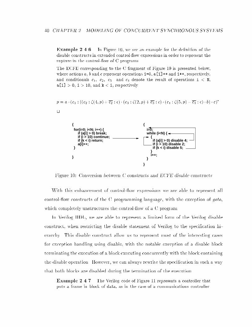
40 CHAPTER 2. MODELING OF CONCURRENT SYNCHRONOUS SYSTEMS
Example 2.4.6. In Figure 10, we see an example for the de�nition of the
disable constructs in extended control- ow expressions in order to represent the
rupture in the control- ow of C programs.
The ECFE corresponding to the C fragment of Figure 10 is presented below,
where actions a, b and c represent operations i=0, a[i]++ and i++, respectively,
and conditionals c1; c2; c3 and c4 denote the result of operations i < N,
a[i] > 0, i > 10, and k < i, respectively.
p = a � (c1 : ((c2 : �(4; p) + c2 : �) � (c3 : �(2; p) + c3 : �) � (c4 : �(5; p) + c4 : �) � b) � c)�
2
for(i=0; i<N; i++) { if (a[i] > 0) break; if (i > 10) continue; if (k < i) return; a[i]++;}
{
}
{
}
i=0;while (i<N) { { if (a[i] > 0) disable 4; if (i > 10) disable 2; if (k < i) disable 5; } i++;}
Figure 10: Conversion between C constructs and ECFE disable constructs
With this enhancement of control- ow expressions we are able to represent all
control- ow constructs of the C programming language, with the exception of goto,
which completely unstructures the control- ow of a C program.
In Verilog HDL, we are able to represent a limited form of the Verilog disable
construct, when restricting the disable statement of Verilog to the speci�cation hi-
erarchy. This disable construct allow us to represent most of the interesting cases
for exception handling using disable, with the notable exception of a disable block
terminating the execution of a block executing concurrently with the block containing
the disable operation. However, we can always rewrite the speci�cation in such a way
that both blocks are disabled during the termination of the execution.
Example 2.4.7. The Verilog code of Figure 11 represents a controller that
puts a frame in block of data, as in the case of a communications controller.

2.4. EXTENDED CONTROL-FLOW EXPRESSIONS 41
fork : BLK_0 begin : BLK_00 while (pce) @(posedge clk) out = preamble; out = sfd; out = destination[0]; out = destination[1]; out = source[0]; out = source[1]; out = length; i = 0; while (length > 0) begin @ (posedge clk) out = data[i]; i = i + 1; length = length + 1; end out = eof; disable BLK_0; end begin : BLK_01 wait (posedge CCT); disable BLK_0; endjoin
o1o2o3o4o5o6o7i1
o8i2l1
o9
Figure 11: Exception handling in Verilog HDL
This code contains two concurrent parts, a sequential code and an exception
handler. The �rst block executes a sequential code which puts the frame on the
data block and transmits it to an output port. The second block disables the
�rst one if signal CCT becomes true while executing block BLK 00, indicating
that the transmission has been interrupted. Conditional len corresponds to the
result of the comparison length > 0.
The ECFE for this Verilog is presented below, where p00 is the ECFE for block
BLK 00 and p01 is the ECFE for block BLK 01.
p = (p00kp01)
p00 = ((pce : o1)� � o2 � o3 � o4 � o5 � o6 � o7 � i1 � (len : o8 � i2 � l1)
� � o9 � �(2; p))
p01 = ((CCT : 0)� � �(2; p))
2
It is worth noting that this type of exception handling mechanism �ts perfectly
well into the framework of other languages for reactive systems, such as Esterel [BS91]
or StateCharts [DH86].

42 CHAPTER 2. MODELING OF CONCURRENT SYNCHRONOUS SYSTEMS
2.4.2 Basic Blocks
The de�nition of control- ow expressions presented in Section 2.2 presents some de-
�ciencies for representing data ow graphs, i.e., graphs that can not be easily repre-
sented by series-parallel compositions of control- ow expressions. One of the possible
ways of representing data ow graphs is the enumeration of all paths of the graph,
making these paths sequential compositions of CFEs, and composing them in parallel,
with the proper synchronization. This approach, however, makes the representation
of data ow blocks ine�cient, since it will increase the complexity of the control- ow
expression representation. We propose in this section the addition of blocks to the
algebra of control- ow expressions in order to e�ciently encapsulate data ow graphs.
De�nition 2.7 Let A be a set of actions, and let the relation!: A�Z�A represent
precedence constraint between two actions, where Z is the set of integer numbers.
Then, a1n! a2 corresponds to specifying that action a1 must be executed at least n
cycles before action a2.
In the de�nition of a precedence constraint, we will use the shorthand notation
a1! a2 whenever n is 1.
Having de�ned precedence constraints enables us to de�ne a basic block as one of
the possible compositions for control- ow expressions.
De�nition 2.8 Let ri be a precedence constraint. A basic block is an extended control-
ow expression represented by the set of precedence constraints fr1; r2; . . . ; rmg.
Note that this basic block can always be represented by the enumeration of all
paths, thus, the basic block de�nition in extended control- ow expressions only adds
a compact and e�cient representation for data ow representations. We will denote a
generic basic block by fRg.

2.4. EXTENDED CONTROL-FLOW EXPRESSIONS 43
m1 m2
m3
m4
m5
a1
lt
m6
a2
s1
s2
Figure 12: Data ow for Di�erential Equation Fragment
Example 2.4.8. The data ow graph of Example 2.2.2 is presented in
Figure 12. This data ow can be represented by the extended control- ow ex-
pression fm1 ! m3; m2 ! m3; m4 ! m5; m6 ! a2; a1 ! lt;m3 ! s1; s1 !
s2; m5! s2g.
If the actions corresponding to multiplications executed in two cycles, and all
other actions executed in one cycle, then the basic block representing this new
set of precedence constraints is given below:
fm1
2! m3; m2
2! m3; m4
2! m5; m6
2! a2; a1 ! lt;m3
2! s1; s1 ! s2; m5
2! s2g
2
2.4.3 Register Variables
In order to de�ne the last extension to control- ow expressions, let us consider Fig-
ure 13. If we adopt the conventional control- ow/data ow partitioning paradigm,
variable state is placed into the data ow. Note, however, that this variable is not
connected with any other part of the data ow, yet it triggers the execution of some
parts of a control- ow expression. This means that if we move variable state into
the control- ow, the communication between the control- ow and data ow will be
reduced. This has some advantages from a synthesis perspective. First, since the
state variable is now incorporated into the control- ow, the redundancy of control in
the data ow can be eliminated, thus reducing the size of the �nal implementation.

44 CHAPTER 2. MODELING OF CONCURRENT SYNCHRONOUS SYSTEMS
Second, when imposing constraints to the design, we will have a more accurate ex-
ecution model for the control- ow, which will be more independent on the data ow
abstraction.
reg [4:0] state;...state = ‘RESET;while ( loop condition )
pncn
c
state
c1
cn
c
p1
pn
DATAFLOW
case (state) ‘RESET: begin state = ‘CASE1; end ‘CASE1: begin state = ‘CASE2; end ‘CASEn: begin state = ‘RESET; end endcaseend
c0
c1
...(c:(c0:p0 + c1:p1 + ... + cn:pn))*...
p0
p1
p0
c0
Figure 13: Program-State Machine Speci�cation
Control- ow/data ow transformations have been regarded in the past as useful
transformations [DDT83, Sta70, DGL92]. However, only ad hoc methods were pre-
sented, and it was claimed that these transformations would probably increase the
number of states of the control.
We will �rst de�ne a reduced dependency graph below, whose structure will allow
us to determine which variables should be moved to the control- ow.
Let Df be the set of data ows of a speci�cation.
De�nition 2.9 A reduced dependency graph is the undirected graph Gr = (Vr; Er),
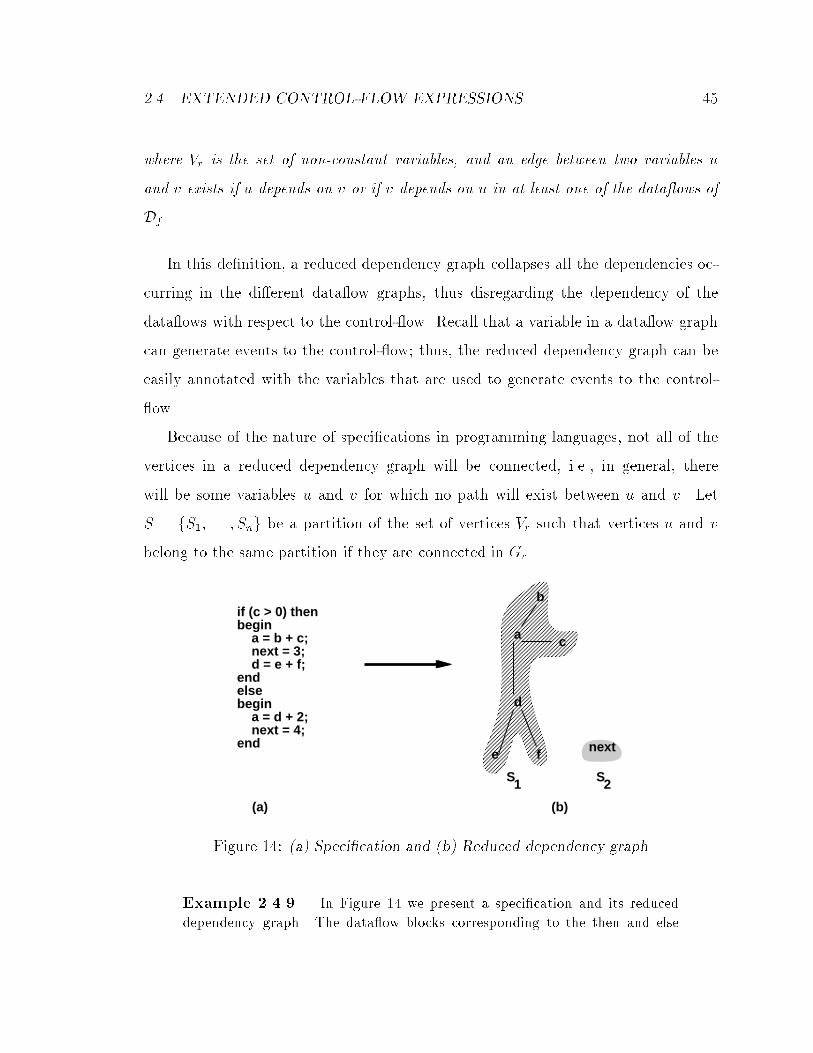
2.4. EXTENDED CONTROL-FLOW EXPRESSIONS 45
where Vr is the set of non-constant variables, and an edge between two variables u
and v exists if u depends on v or if v depends on u in at least one of the data ows of
Df .
In this de�nition, a reduced dependency graph collapses all the dependencies oc-
curring in the di�erent data ow graphs, thus disregarding the dependency of the
data ows with respect to the control- ow. Recall that a variable in a data ow graph
can generate events to the control- ow; thus, the reduced dependency graph can be
easily annotated with the variables that are used to generate events to the control-
ow.
Because of the nature of speci�cations in programming languages, not all of the
vertices in a reduced dependency graph will be connected, i.e., in general, there
will be some variables u and v for which no path will exist between u and v. Let
S = fS1; . . . ; Sng be a partition of the set of vertices Vr such that vertices u and v
belong to the same partition if they are connected in Gr.
if (c > 0) thenbegin a = b + c; next = 3; d = e + f;endelse begin a = d + 2; next = 4;end
a
b
c
d
e f next
S1 S2
(a) (b)
Figure 14: (a) Speci�cation and (b) Reduced dependency graph
Example 2.4.9. In Figure 14 we present a speci�cation and its reduced
dependency graph. The data ow blocks corresponding to the then and else
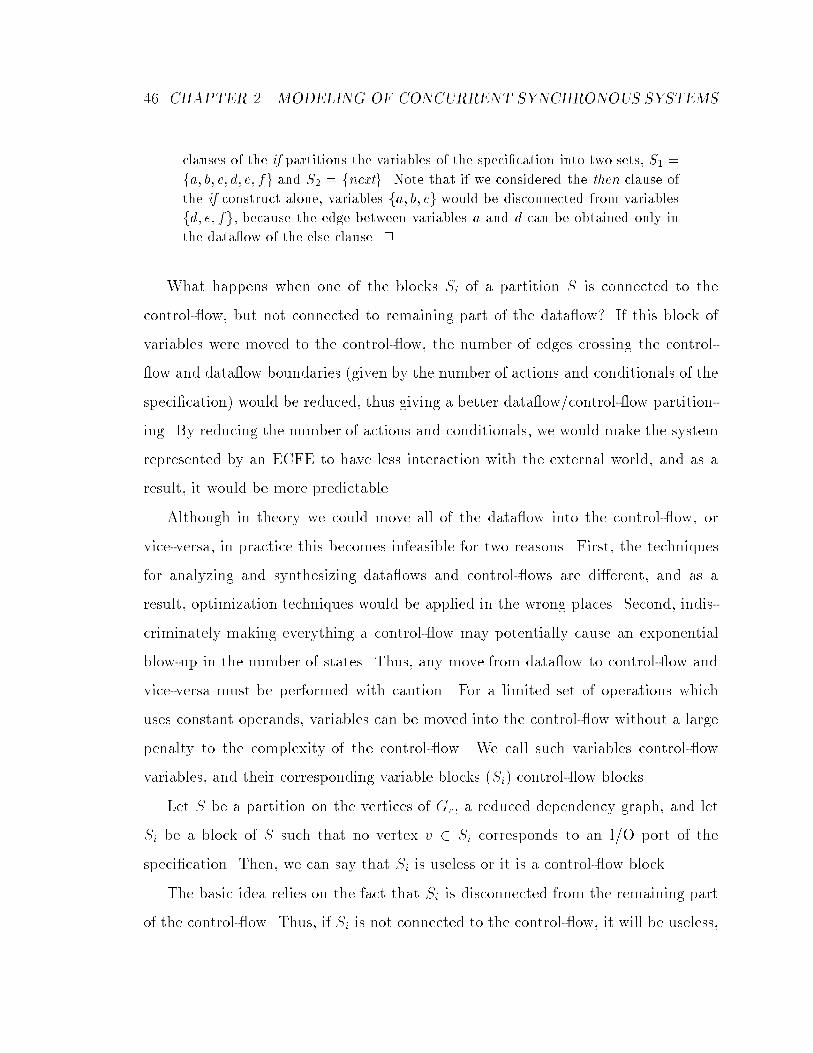
46 CHAPTER 2. MODELING OF CONCURRENT SYNCHRONOUS SYSTEMS
clauses of the if partitions the variables of the speci�cation into two sets, S1 =
fa; b; c; d; e; fg and S2 = fnextg. Note that if we considered the then clause of
the if construct alone, variables fa; b; cg would be disconnected from variables
fd; e; fg, because the edge between variables a and d can be obtained only in
the data ow of the else clause. 2
What happens when one of the blocks Si of a partition S is connected to the
control- ow, but not connected to remaining part of the data ow? If this block of
variables were moved to the control- ow, the number of edges crossing the control-
ow and data ow boundaries (given by the number of actions and conditionals of the
speci�cation) would be reduced, thus giving a better data ow/control- ow partition-
ing. By reducing the number of actions and conditionals, we would make the system
represented by an ECFE to have less interaction with the external world, and as a
result, it would be more predictable.
Although in theory we could move all of the data ow into the control- ow, or
vice-versa, in practice this becomes infeasible for two reasons. First, the techniques
for analyzing and synthesizing data ows and control- ows are di�erent, and as a
result, optimization techniques would be applied in the wrong places. Second, indis-
criminately making everything a control- ow may potentially cause an exponential
blow-up in the number of states. Thus, any move from data ow to control- ow and
vice-versa must be performed with caution. For a limited set of operations which
uses constant operands, variables can be moved into the control- ow without a large
penalty to the complexity of the control- ow. We call such variables control- ow
variables, and their corresponding variable blocks (Si) control- ow blocks.
Let S be a partition on the vertices of Gr, a reduced dependency graph, and let
Si be a block of S such that no vertex v 2 Si corresponds to an I/O port of the
speci�cation. Then, we can say that Si is useless or it is a control- ow block.
The basic idea relies on the fact that Si is disconnected from the remaining part
of the control- ow. Thus, if Si is not connected to the control- ow, it will be useless,

2.4. EXTENDED CONTROL-FLOW EXPRESSIONS 47
since all the values assigned to its variables will not be used anywhere. On the other
hand, if this block of variables is connected to the control- ow, then it will be a
control- ow block.
In the sequel we denote by � = fv; c1; . . . ; cmg a generic connected component
of Vr when ci are Boolean variables. We also denote by R = f=; 6=; <;>;�;�g the
set of relational operations and by � a generic element of R. We also denote by a
constant. The following corollary is used in our extension to control- ow expressions.
Corollary 2.1 Let v and c be variables of the connected component �. Let also f be
either an identity function, an increment or a decrement, and let cj �(v1; . . . ; vn)
and v f(v) be the only operations of the speci�cation de�ned over cj and v. Then,
either Si is a control- ow block or it is useless.
It remains to be seen that such transformations are useful by showing that these
types of speci�cations occur in real designs. It is not hard to see that the variable state
from Figure 13 satis�es the conditions of Corollary 2.1. We present in Figure 15 (a)
the di�erent data ows for the description of Figure 13, and in Figure 15 (b) the
reduced dependency graph for these data ows. Other variables that often occur in
the speci�cations of control-dominated speci�cations are counters, for example.
The observations shown in this section leads to the following extension to control-
ow expressions.
De�nition 2.10 Let � be the connected component of Vr de�ned previously. Then
[v ], [v ++] and [v ��] are extended control- ow expressions, and [�(v; )] is a
guard.
Note that every register variable v 2 Vr is �nite, since the corresponding speci-
�cation has �nite memory in the number of variables. As a result, every operation
performed on the register variable v will be computed over the range f0; . . . ; jvj � 1g,
where jvj is the number of possible values for the register.

48 CHAPTER 2. MODELING OF CONCURRENT SYNCHRONOUS SYSTEMS
state
‘RESET ‘CASE1
state
‘CASE2
state
...
state ‘RESET
c0
==
state
==...
‘CASEn
cn
(a)
state
c0 cn...
(b)
Figure 15: (a) Data ow graphs for program-state machine and (b) reduced depen-
dency graph
We could have extended the model presented above to incorporate more of the
data ow of the speci�cation into the control- ow. However, introducing more vari-
ables into the extended control- ow expressions could easily increase complexity in
the internal representation of the control- ow.
2.4.4 De�nition of Extended Control-Flow Expressions
We can now de�ne extended control- ow expressions, by putting together all the
elements from control- ow expressions with the extensions proposed in this section.
The set of symbols is extended to include registers, i.e., � = A [ C [ R [ F ,
where A is the set of actions, C is the set of conditionals, R is the set of register
variables with a �nite number of possible values and F is the set of process variables.
The set of operations is de�ned as O = f�;+; :; �; !; k; �; [:=]; [++]; [��]; fRgg, where
f�;+; :; �; !; kg are the compositions of control- ow expressions de�ned in Section 2.2,
� is the disable construct, [:=]; [++] and [��] are functions de�ned on registers, and
fRg are basic blocks. The formal de�nition is presented below.
De�nition 2.11 Let (�;O; �; �) be the algebra of extended control- ow expressions
where:

2.4. EXTENDED CONTROL-FLOW EXPRESSIONS 49
� is an alphabet that is subdivided into the alphabet of actions, conditionals,
registers and processes;
O is the set of composition operators that de�ne sequential, alternative, guard,
loop, in�nite, parallel behavior, exception handling, basic blocks and operations
over registers;
� is the identity operator for alternative composition;
� is the identity operator for sequential composition.
Guards in extended control- ow expressions are de�ned also as Boolean functions
over conditionals, but including relational operations between registers and constants.
We can now de�ne a more general form of control- ow expressions, which will be
called in this thesis extended control- ow expressions, or ECFEs.
De�nition 2.12 Extended control- ow expressions are:
� Actions a 2 A.
� Process p 2 F .
� � and �.
� �(n; p), where n is a natural number and p 2 F .
� fr1; r2; . . . ; rmg, where ri is a precedence relation of the form ajn! ak, faj; akg �
A.
� [v := constant]; [v++]; [v ��], where v is a register
� If p1; . . . ; pn are extended control- ow expressions, and c1; . . . ; cn are guards,
then the following expressions are extended control- ow expressions.

50 CHAPTER 2. MODELING OF CONCURRENT SYNCHRONOUS SYSTEMS
{ The sequential composition, represented by p1 � . . . � pn
{ The parallel composition, represented by p1k . . . kpn
{ The alternative composition, represented by c1 : p1 + . . . + cn : pn
{ Iteration, represented by (c1 : p1)�
{ Unconditional repetition, represented by p!1.
Nothing else is an extended control- ow expression.
Unless otherwise stated, we will refer to extended control- ow expressions by
control- ow expressions in the remainder of this thesis.
2.5 Comparison of CFEs with Existing Formalisms
Control- ow expressions are very useful as a modeling and abstraction formalism for
the control- ow of a concurrent system, since the translation from control/data ow
representation into CFEs is straightforward. In this section, we compare CFEs with
other representative formalisms that were used to model the control- ow, while ab-
stracting the data ow information: regular expressions, path expressions, �nite-state
machines, Petri-nets, algebra of concurrent processes (ACP), calculus of communi-
cating systems (CCS), timing expressions, CIRCAL and BFSMs.
� The algebra of regular expressions [Kle56, HU79] is used to represent strings
accepted or emitted by a �nite-state machine. This algebra is represented by
(�;+; �; �), where � is the alphabet of characters accepted/emitted, + denotes
alternative composition, � denotes sequential composition, and � denotes zero
or more repetitions of a subexpression.
Regular expressions have been used in the modeling of the control- ow of se-
quential programs [Pai77, Las90]. In [TU82], regular expressions were used as

2.5. COMPARISON OF CFES WITH EXISTING FORMALISMS 51
a speci�cation language for �nite-state machine recognizers. In order to spec-
ify the control- ow in terms of an input/output behavior, regular expressions
must be extended to guard alternative branches and loops. Also, in the case of
parallel descriptions, a parallel operator must be added. However, this parallel
operator is redundant for regular expressions, since the left and right distribu-
tivity of the sequential operator with respect to the alternative operator allow
concurrency to be traded by non-determinism [Mil84]. Such expressiveness does
not exist in control- ow expressions, because the sequential operator does not
distribute to the right with respect to the alternative operator, a requirement
for a system to react correctly to its environment.
CFEs also extends regular expressions by de�ning in�nite behaviors, which
could be achieved only by extending regular expressions to !-regular expres-
sions [Cho74], by breaking the normal ow of execution by means of the disable
construct, and by allowing certain variables from the data ow to be incorpo-
rated into the control- ow.
� Path expressions [Cam76] are equivalent to regular expressions, with the ad-
dition of parallelism. However, instead of a synchronous execution semantics for
the parallel composition, path expressions assume an interleaved execution se-
mantics. Control- ow expressions extend path expressions by providing guards
to alternative branches and loops, in the same way CFEs extended regular
expressions. CFEs also breaks the ow of control with the disable construct
and it allows certain variables from the data ow to be incorporated into the
control- ow.
� A �nite-state machine [Mea55, Moo56, HU79] recognizer is a tuple (�;S; �; S0;
F ), where � is a set of inputs, S is the set of states, � : S � � ! S is the
transition function, S0 is the set of initial states, and F is the set of �nal states.

52 CHAPTER 2. MODELING OF CONCURRENT SYNCHRONOUS SYSTEMS
In the case of �nite-state machines as computational engines, we also de�ne
an output alphabet O, and either the output transition function � : S ! O
(in the case of a Moore machine) or � : S � � ! O (in the case of a Mealy
machine). Parallelism in �nite-state machines is de�ned only at the transition
level, in which several outputs may be generated at the same time. At this level,
however, the duration for each output has already been determined, and any
transformation of the speci�cation that modi�es this execution time cannot be
performed.
A speci�cation consisting of a set of concurrently executing �nite-state machines
can also be considered in this model, as in the case of reactive system languages,
such as StateCharts [DH86] and SDL [Sar89]. In these languages, the system
is modeled as a set of hierarchical concurrent �nite-state machines, and the
system's state is de�ned to be the state of the cartesian product of all concur-
rently executing �nite-state machines. As in the case described in the previous
paragraph, at the level of �nite-state machines, the execution time for the oper-
ations has already been decided, and thus any transformation that changes the
execution time of operations cannot be performed, without requiring a restruc-
turing of the �nite-state machine. Furthermore, a �nite-state machine model
attens the hierarchy present in the control- ow, thus preventing any control-
optimization technique based in control- ow hierarchy [KM92] to be used.
� Petri nets [Pet81] are represented by the tuple (T; P; �; I), where T is the set of
transitions, P is the set of places, and � � T �P [P �T de�nes the transition
relation (or �ring) from transitions to places and vice-versa. A marking in
Petri-nets is an assignment of natural numbers (tokens) to places. I is the
initial marking of the Petri-net.

2.5. COMPARISON OF CFES WITH EXISTING FORMALISMS 53
A state in a Petri-net is a marking of places. Transitions between states are
achieved by having a marking that becomes another marking by �ring some
transition. This �ring occurs when one transition of the net has all incoming
places with more than one token. The transition takes one such token from
each place and puts one additional token in every outgoing place. Since only
one �ring can occur at any time, this model can only represent interleaved
concurrent systems.
One possible extension of Petri-nets is the synchronous �ring semantics [Wan88].
In this semantics, the set of �rings that can occur at the same time is speci�ed
along with the Petri-net. Similarly to the concurrent �nite-state machine model,
any transformations that changes the execution time of the operations, or the
structure of the graph cannot be easily performed.
Whereas Petri-nets only have a graphical representation, control- ow expres-
sions views the system in an algebraic way, presented in this chapter, and in
a graphical representation as a �nite-state machine, which will be presented
in Chapter 4. A dual view allows the analysis of a concurrent system to be
performed at two levels of abstraction. In the algebraic view, we analyze the
system by using its hierarchy (in terms of uplevels of a CFE) to abstract \un-
interesting" portions of the computation. In the graphical representation, we
perform reachability analysis that enables us to reason about the system as a
whole. Together, these two procedures can be more e�cient than just a graph-
ical representation. Similar to CFEs, Garg et. al. [GG92] de�ned concurrent
regular expressions as an algebraic model for Petri-nets. One of the key dif-
ferences between CFEs and concurrent regular expressions is that the former
will be able capture more succinctly the control- ow of systems described by
hardware description languages and programming languages.

54 CHAPTER 2. MODELING OF CONCURRENT SYNCHRONOUS SYSTEMS
� Process algebra [Bae90] and CCS [Mil91] correspond to a family of represen-
tations used to formally model concurrent systems. In these models, we view
the system as a set of operations that are represented by actions, and their
compositions in terms of sequential composition, non-deterministic choice, par-
allel composition and communication. Concurrency usually refers to interleaved
concurrency, which is represented by non-deterministic choice; and synchronous
concurrency is de�ned in terms of communication.
These representations can be considered as a superset of control- ow expres-
sions. If we restrict the set of speci�able behaviors to regular and synchronous
processes, then control- ow expressions will have the same representation capa-
bilities of process algebras and CCS. One of the unique features of control- ow
expressions that was de�ned previously in this paper is that we distinguish ac-
tions from conditionals. This allows the system to better capture the reactive
nature of hardware systems, and as a result, control- ow expressions will �t
better the model used for synthesis.
When compared to the extensions to control- ow expressions presented in Sec-
tion 2.4, we see that CFEs gives more exibility to encapsulate the control- ow
behavior present in systems that needs to react to its environment, sometimes
in a non-structured way, such as with exception handling mechanisms or by
representing state variables.
� Timing expressions [ZJ93a, ZJ94] is a model for describing behaviors of se-
quential systems and specifying sequential constraints a sequential system has
to satisfy [ZJ93a]. In timing expressions, the sequential system is represented
by expressions that may take di�erent values over time. When compared to
control- ow expressions, we see that timing expressions will be better suited
to represent the control information at lower levels of descriptions, whereas

2.5. COMPARISON OF CFES WITH EXISTING FORMALISMS 55
control- ow expressions will be better suited for representing the control- ow
at higher-levels of descriptions. In addition to that, control- ow expressions
can be considered as a superset of timing expressions, since CFEs can represent
systems containing hierarchical series-parallel speci�cations, whereas in timing
expressions parallelism can occur only at the highest level.
� CIRCAL [Mil85, Mil94] is a model for concurrent systems in which alternative
behavior and non-deterministic choice is represented separately. The represen-
tation of a concurrent system in CIRCAL consists of a set of labels executing
concurrently | thus this model supports true concurrency | and the opera-
tions among these models, including sequential, alternative, non-deterministic
choice, concurrency and communication, which is achieved by matching labels
of a CIRCAL description.
When representing a reactive system, CIRCAL does not distinguish the inputs
from the outputs of the system. Thus, we can view a CIRCAL description as
a high-level view of the interactions that occur in a system, without worrying
about how these interactions take place. In CFEs, we represent the interactions
of the inputs and the outputs in a system di�erently. Inputs of CFEs compose
using regular Boolean laws, and are assumed to execute in zero time, whereas
outputs of CFEs compose through synchronization, similar to the composition
rules for CIRCAL.
� BFSMs [WTL91] are a generalization of �nite-state machines with partial tim-
ing information on the relative execution time of the states. This model closely
resembles the algebra of control- ow expressions because it was used for mod-
eling and synthesis of control-dominated speci�cations. However, the lack of a

56 CHAPTER 2. MODELING OF CONCURRENT SYNCHRONOUS SYSTEMS
synchronization 3 formalism and the lack of a formal model for constraint speci-
�cation | which is restricted to scheduling constraints | prevents BFSMs from
being used in more complex problems. As opposed to CFEs, which uses both
expression and �nite-state machine representations for a concurrent system, the
translation from the speci�cation to a �nite-state machine description is per-
formed too early with BFSMs, and thus, optimizations that would be best used
at the expression level | such as hierarchical abstraction and rewriting | are
not available to the synthesis process. Finally, a BFSM is a model best suited
for representing the control- ow of languages in which parallelism is speci�ed
at the process level, such as VHDL. If used to represent the control- ow of lan-
guages that can specify series-parallel composition of systems, such as Verilog
HDL, its representation and constraint speci�cation becomes cumbersome.
When compared to the formalisms presented above, control- ow expressions are
able to capture more succinctly the control- ow information, abstraction from the
original speci�cation, and the degrees of freedom. When considering speci�cations in
terms of control/data ow abstractions | or in terms of the corresponding HDL code
| control- ow expressions �t perfectly as a modeling tool of the control behavior for
synthesis of system-level speci�cations.
2.6 Summary
In this section we presented a model for representing the behavior of a control-
dominated concurrent system. This model was called the algebra of control- ow
expressions, and its axioms were presented along with a discussion of its limitations
for representing the control- ow of structured programs.
3We will de�ne formally synchronization in the next chapter.

2.6. SUMMARY 57
We also provided extensions to the algebra of control- ow expressions so that we
are able to represent exception handling, basic blocks and a limited form of register
variables. Exception handling was introduced to overcome the limitation of a single-
exit point from the structured compositions of CFEs, thus allowing us to represent the
disruption of control. Basic blocks were de�ned to reduce the complexity for repre-
senting general dependency structures corresponding to basic blocks in programming
languages. Register variables enriched control- ow expressions by enabling the repre-
sentation of more diverse control- ow structure, such as in the case of a program-state
machine. We showed how to systematically repartition the control- ow and data ow
portions in order to reduce the communication between control- ow and data ow,
thus creating a more accurate execution model for the control- ow when we abstract
the data ow.
These extensions allowed us to express e�ciently most of the control- ow from
structured programming languages and hardware description languages.
In the next chapter, we will focus on the analysis of a system modeled by control-
ow expressions.

Chapter 3
Modeling the Environment
Characterizing a system for synthesis implies modeling the design and the environ-
ment surrounding it. We modeled the design in the previous chapter with CFEs. In
this chapter, we will show how the environment can be represented using CFEs.
At the higher levels of abstraction, the speci�cation is non-deterministic, because
at this level we like to encapsulate multiple design choices of the system. This non-
determinism is resolved during the synthesis of control-units by selecting a determinis-
tic implementation that optimizes a design goal. As a result, we will have to uniquely
identify the non-deterministic choices of the design when we model the system's non-
determinism. This will be achieved by guarding CFEs with decision variables.
Since the speci�cation of the environment surrounding a speci�cation is a formidable
task, we will be providing methods for abstracting the environment. In particular, we
will be interested in abstractions that can be used for scheduling operations statically
in basic blocks, and in abstractions that can be used to synchronize the concurrent
parts of the design. Among these abstractions, we will show how to represent the
environment's timing, resource usage and synchronization constraints.
58

3.1. QUANTIFICATION OF THE DESIGN SPACE 59
3.1 Quanti�cation of the Design Space
In this section, we will show how decision variables can be used to quantify the design
space. Let us begin by de�ning what is a decision variable.
De�nition 3.1 A decision variable x is a variable guarding the execution of a control-
ow expression whose value is determined by the synthesis procedure. Its possible
values are de�ned as the set of Boolean formulas over some set D.
A decision variable is a Boolean variable quantifying implementation choices for
control- ow expressions. They can be assigned either constant values or Boolean
functions over a set D. At this point, we have to distinguish among these two types
of assignments, and where they appear in control- ow expressions.
a
Static Dynamic
x1 x2
a
a
1 0
a
a
c c
Figure 16: Static and dynamic decision variables
We call static decision variables the decision variables that are assigned constant
values, and dynamic decision variables the decision variables that are assigned the
Boolean functions over D. Figure 16 shows the di�erence between static and dynamic

60 CHAPTER 3. MODELING THE ENVIRONMENT
decision variables. We assume that x1 and x2 are decision variables that will determine
when some action a will be executed. If x1 and x2 are static decision variables, they
will be assigned constant values such that only one of the possible executions for
action a will be selected during synthesis. If x1 and x2 are considered to be dynamic
decision variables, then both schedules are possible, and the selection will be made
at execution time, based on some input c.
Although it may seem that it is always better to use dynamic decision variables,
the algorithms for assigning values to them are not as e�cient as the algorithms used
for assigning values to static decision variables. As a result, we use both static and
dynamic decision variables in CFEs.
Static decision variables are used to identify possible schedules for the operations
inside basic blocks of CFEs. We will assume that basic blocks will encapsulate a set of
operations (represented by the respective actions) that must be scheduled statically
with respect to the beginning of the basic block.
Recall that a basic block is represented by a set of precedence constraints. Ac-
cording to these precedence constraints and to the maximum allowed time to execute
a basic block, each operation of the basic block will have a set of possible times it can
execute relative to the beginning of the basic block.
We annotate each possible execution time of an operation inside its basic block
with a static decision variable, and this decision variable will uniquely identify when
the operation will be executed. Suppose an operation oi can be executed at times
fj1; . . . ; jng. Then, we create n decision variables for the operation oi, namely
xij1; . . . ; xijn. If xij1 is one, operation oi is executed at time j1.
We will also introduce a decision variable for each possible execution time of the
basic block because a constraint satisfaction may require a basic block to execute
beyond the minimum time necessary to execute its operations.

3.1. QUANTIFICATION OF THE DESIGN SPACE 61
m1 m2
m3
m4
m5
s1
s2
m1 m2
m3 m4
m5s1
s2
(a) (b)
Figure 17: Minimum (a) and maximum (b) execution times for the operations of the
di�erential equation CDFG
Example 3.1.1. Static Decision Variables: Figure 17 presents the
minimum (a) and maximum (b) execution times for a part of the control-data
ow graph of the di�erential equation solver of Example 2.3.2. In this example,
we restricted the maximum execution time for the basic block to four cycles.
The basic block representing the system is given by fm1 ! m3; m2! m3; m4 !
m5; m3! s1; s1 ! s2; m5 ! s2g.
In Figure 17, since action m1 can only be executed in the �rst cycle, it only
requires one decision variable, xm1. For action m4, we represent the design
space using two decision variables, xm4;1 and xm4;2. If xm4;1 is true, then
operation m4 is executed in the �rst cycle of the basic block. If xm4;2 is true,
then operation m4 is executed in the second cycle. The decision variables for
the other actions can be obtained in a similar manner.
In addition to the decision variables de�ned in the previous paragraph, we
also de�ne four decision variables corresponding to the four cycles of the basic
block, namely decision variables y1, y2, y3 and y4. If yi is true, for example, the
basic block must execute in exactly i cycles, independent on the execution time
necessary to execute the operations of the basic block. In this case, it should
be clear that y4 will be always true, and y1, y2 and y3 will be false. If we had
chosen a basic block executing in at most 5 cycles, then either y4 or y5 could
be true. 2
We also introduce decision variables outside the scope of basic blocks. These deci-
sion variables will be called dynamic decision variables and they will be dynamically
satis�able. They will be assigned Boolean functions whose truth values change over

62 CHAPTER 3. MODELING THE ENVIRONMENT
time. In the following chapters, we will see that the assignment to these variables
will consider the \state" of the system being synthesized, and this will enable us
to synchronize the concurrent parts of the speci�cation with respect to the design
constraints.
Since static decision variables are only used to identify possible schedules inside
basic blocks, and dynamic decision variables will be used elsewhere in the speci�ca-
tion, we will refer to both as decision variables, and it will be clear from the context
which type of decision variable we are referring to.
In control- ow expressions, decision variables can be used as guards of expressions,
so we extend guards to allow decision variables and conditionals to be composed
together.
De�nition 3.2 A guard is a Boolean formula over the set of decision variables and
the set of conditionals.
Example 3.1.2. Dynamic Decision Variable: Consider the code
w = y � z; u = w + 3;. Assume both the multiplication and the addition take
one clock cycle, and that w = y � z is represented by action a and u = w + 3
is represented by action b. A constraint between a and b, or the quanti�cation
of all possible schedules such that b occurs after a is represented by the CFE
a � (x : 0)� � b, where a; b 2 A, and x is a decision variable. In this CFE, the
possible schedules are quanti�ed by the di�erent assignments of the decision
variable x over time.
Possible assignments could be:
a � b
a � 0 � b
a � 0 � 0 � b...
a � 0 � � � � � 0 � b
The �rst assignment corresponds to an assignment of x to false after the exe-
cution of action a. The second assignment corresponds to an assignment of x

3.2. CONSTRAINT SPECIFICATION 63
to true after the execution of a, then to false. The other assignments have a
similar correspondence. 2
Note the structure imposed by allowing dynamic decision variables in CFEs, and
static decision variables in basic blocks. During synthesis, operations inside basic
blocks are statically scheduled with respect to the beginning of the basic block, which
can be dynamically synchronized with other parts of the design by guarding the
basic block's execution with dynamic decision variables. In the context of pipelines,
[HB84] presented a similar structure to dynamically recon�gure the initiation rate for
multi-function pipelines.
In the following section, we will show how CFEs and decision variables can be
used to represent the design constraints.
3.2 Constraint Speci�cation
Constraints are properties that any implementation needs to satisfy. In general,
the system being synthesized needs to communicate with the external environment,
or with custom made components, for which an interface has been speci�ed. The
interface properties must be satis�ed in all valid implementations for the system to
work properly. In addition to interface constraints, the user may impose structural
constraints that will limit the degrees of freedom used to implement a behavior. For
example, the user may limit a design to use a single bus for communication with the
other models.
Since specifying the environment under which a system is going to execute is
formidable task, several approaches have been proposed in the past to specify the
system's constraints. In [NT86, KM92, Bor88, HLH91, RB93], the environment's
constraints were speci�ed as minimum or maximum timing constraints between two

64 CHAPTER 3. MODELING THE ENVIRONMENT
operations. Since the algorithms for �nding schedules satisfying those timing con-
straints were limited to basic blocks, these timing constraints were limited to opera-
tions in the same basic block. This prevented designers from specifying more complex
interactions existing in control-dominated speci�cations, such as timing constraints
in alternative paths or loops.
More recently [TWL95], the environment's timing constraints have been extended
to allow minimum and maximum timing constraints on arbitrary paths in the speci�-
cation, and in [YW] an algorithm was proposed that obtains schedules satisfying these
timing constraints. Using this new formulation, for example, the user can constrain
the execution time for the hit-case of a cache controller, while using a di�erent timing
constraint for the miss-case of the same cache controller. Note however, that since the
hit and miss cases belong to the same description and share parts of the speci�cation,
these shared parts will be constrained by the hit and miss timing constraints.
The set of timing constraints specifying the interactions between the system and
its environment can become unmanageable in some designs because of the number of
interactions among the di�erent parts, as in the case of a model whose environment
is a bus protocol or in the case we want to synthesize protocol converters between
two speci�cations. Thus, we need to extend the methods for specifying constraints
presented above by allowing the system to be described as a parallel composition of
the speci�cation and a suitable representation of the environment.
Figure 18 depicts the representation a process P corresponding to a circuit spec-
i�cation, and its environment, represented by process Env. Note that all timing con-
straints are encapsulated by process Env which synchronizes with the speci�cation
for P . Thus, the system under consideration for synthesis purposes is represented by
the CFE pjje, where p is the control- ow expression for P and e is a CFE representing
a suitable model for P 's environment.

3.2. CONSTRAINT SPECIFICATION 65
P
Env
Figure 18: Process P and its Environment
Note that we do not restrict our discussion to timing constraints in the speci-
�cation of the environment, but we also allow the environment to contain resource
usage constraints and synchronization constraints. These types of constraints are
used in this section as building blocks to construct more complex constraints with
control- ow expressions.
The reader must keep in mind the the goals in the synthesis ow. We want to
solve two problems: statically scheduling the operations inside basic blocks using
these system's constraints, and dynamically synchronizing the parts for which no
static schedule can be found. This yields two types of constraints that will be han-
dled di�erently during synthesis for e�ciency reasons: statically satis�able constraints
which constrain the operations inside a basic block, and dynamically satis�able con-
straints, which require the synthesis of synchronization skeletons for the process being
synthesized.
We will �rst present dynamically satis�able constraints, which uses compositions
of control- ow expressions. Then, we will de�ne statically satis�able constraints as a
subset of dynamically satis�able constraints.

66 CHAPTER 3. MODELING THE ENVIRONMENT
3.2.1 Dynamically Satis�able Constraints
In this section, we begin by presenting the speci�cation of constraints that can be
dynamically satis�able. We consider here a subset of constraints that can be speci�ed
as scheduling constraints, binding constraints and synchronization constraints. More
complex speci�cations can be achieved by composing these constraints using control-
ow expressions.
Timing constraints are de�ned in terms of control- ow expressions. In binding
constraints, we use expression rewriting, i.e., the incorporation of binding constraints
as a modi�cation of the original CFE. Both timing and binding constraints use deci-
sion variables as quanti�ers of the design space. Finally, synchronization constraints
use multisets of actions that should occur at the same time and multisets of actions
that should never occur at the same time.
Dynamically satis�able constraints are de�ned in terms of the actions that appear
in a control- ow expression, which we de�ne below as the support of a CFE.
De�nition 3.3 The support of a control- ow expression p is de�ned as the set of
actions that are executed in p.
Example 3.2.3. The support of a CFE p = (a � b)!jj(c � d � e)!, written as
Sp, is the set of actions of p. Here, Sp = fa; b; c; d; eg. 2
Associated with each action de�ned in the support of a CFE, we have a shadow
action, which executes every time the corresponding action executes.
De�nition 3.4 A shadow of an action a, written as �a, is de�ned to be an action
that does not correspond to any operation of the original speci�cation and executes
every time action a is executed.
Example 3.2.4. In the CFE (a � b � c)!, �a, �b and �c execute every time a,
b and c are executed, respectively. 2

3.2. CONSTRAINT SPECIFICATION 67
Scheduling Constraints
Scheduling constraints are constraints that specify the timing relations among com-
putations. Although we will only de�ne minimum and maximum timing constraints
here, we can specify and handle a much richer set of constraints with control- ow ex-
pressions, including loops, alternative composition and synchronization, as opposed
to the constraints that are handled in other CAD tools, such as [TWL95, WTHM92,
KM92, Bor88]. The speci�cation of scheduling constraints using control- ow expres-
sions can be also considered as an extension of path constraints de�ned by [TWL95].
Let us assume p to be a CFE representing a speci�cation of a design with support
Sp. Suppose we want to represent initially simpleminimumand maximumconstraints
between two actions a and b, with a; b 2 Sp.
De�nition 3.5 A minimum timing constraint of n cycles between two actions a and
b, whose shadow actions are �a and �b, can be represented by the CFE (x : 0)� � �a �
0n�1 � (y : 0)� � �b, where x and y are decision variables.
In this de�nition for minimum timing constraint, the CFE waits until action a
executes by setting x to true for multiple cycles. Then, it counts n� 1 cycles (0n�1)
and waits for action b to execute, which represented by b's shadow action �b.
De�nition 3.6 A maximum timing constraint on n cycles between two actions a and
b, whose shadow actions are �a and �b, can be represented by the CFE (x : 0)� ��a �(y :
0)<n � �b, where x and y are decision variables.
The constraint de�ned above de�nes a maximumtime between two actions by �rst
waiting for action a to execute, represented by its shadow action, and then waiting at
most n�1 cycles until it allows action b to execute, by synchronizing with b's shadow
action.

68 CHAPTER 3. MODELING THE ENVIRONMENT
The following theorem shows how to combine the two de�nitions in order to obtain
a timing constraint de�ned as the delay between two actions.
Theorem 3.1 Let min = (x1 : 0)� � �a � 0n�1 � (x2 : 0)� � �b be a minimum timing
constraint of n cycles between a and b, and let max = (x3 : 0)� � �a � (x4 : 0)<n � �b be a
maximum timing constraint of n cycles between a and b, where x1, x2, x3 and x4 are
decision variables. The CFE minkmax is the timing constraint representing exactly n
cycles between a and b, which can be rewritten as (y : 0)� � �a � 0n�1 � �b, where y is a
decision variable.
Proof: Note that x1 and x3 will have the same assignment over time, since
they will be synchronizing with the execution of �a, and this assignment
will be the same as the assignments over time for y for the same reason.
Because the execution of b in both constraints is synchronized to the
execution of the respective shadow actions, x2 will always be assigned to
0, and x4 will be assigned 1 in the �rst n � 1 cycles, and then 0. If we
substitute these assignments to x3 and x4, we obtain (y : 0)� ��a �0n�1 ��b.
]
We can now de�ne the representation of a system and the environment speci�ed
in terms of timing constraints and the auxiliary actions.
De�nition 3.7 Let p be a control- ow expression modeling a system, and let m1; . . . ;
mn be a set of CFEs representing scheduling constraints from the environment. The
control- ow expression pjjm1jj � � � jjmn denote the system consisting of p and its en-
vironmental constraints. We call this new expression the application of timing con-
straints to p.
Example 3.2.5. In the di�erential equation solver of Example 2.3.1, assume
the CFE for the speci�cation is p, and that we want to specify a maximum
timing constraint of 3 cycles between m4 and s2, which can be represented by
the CFE (x1 : 0)� � �m4
� (x2 : 0)<3 � �s2 , where x1 and x2 are decision variables.
The application of this constraint to the CFE p is represented by a new CFE
pjj(x1 : 0)� � �m4
� (x2 : 0)<3 � �s2 . 2

3.2. CONSTRAINT SPECIFICATION 69
In the previous example, we speci�ed conventional minimumand maximumtiming
constraints. As we pointed out before, CFEs can be used to specify a much broader
set of scheduling constraints, and even hide interface information from the original
speci�cation, as shown in the following example.
Example 3.2.6. In the di�erential equation solver of Example 2.3.1, let
p be the process representing the CFE for the basic block. For the CFE q =
((x1 : 0)� �a �p)!jj((x2 : 0)
� �b �p)!, the constraint (x : 0)� ��a � (c : 02+ c : 03) ��b
indicates that the �rst basic block should execute either 2 cycles or 3 cycles
before the second one, depending on the conditional c. 2
Binding Constraints
Binding constraints specify the possible implementations for each computation that
is represented by an action. We represent binding constraints as a rewriting of the
original control- ow expression.
De�nition 3.8 Let p be a control- ow expression with support Sp. A rewriting of
p, written as R(p)[a q], where q is a control- ow expression, is de�ned as the
substitution of every occurrence of a 2 Sp in p by q.
Example 3.2.7. Assume we make the rewriting of a by (c1 : a0 � a1 + c2 :
a0 � a1 � a2) into p = (a � b)!jj(c � d � e)!. Then:
R(p)[a (c1 : a0 �a1+c2 : a0 �a1 �a2)] = ((c1 : a0 �a1+c2 : a0 �a1 �a2)�b)!jj(c�d�e)!
2
De�nition 3.9 Let p be a CFE of a speci�cation and assume some action a can
be implemented by a set of components fC1; C2; � � � ; Cmg. This binding constraint is
represented by the CFE:
R(p)[a X
1�i�m
xi : Ci]
whereP
1�i�m xi : Ci represents the alternative composition of the m terms (xi :
Ci), and x1; � � � ; xm are m decision variables.

70 CHAPTER 3. MODELING THE ENVIRONMENT
In this expression rewriting, whenever xi is true, component Ci implements the
computation abstracted by action a. Note that since decision variables are assumed
to take values from the set of Boolean formulas over D, and not just the values 0
or 1, we may have an implementation in which some xi enables component Ci at
some time, and at a later time xj (i 6= j) enables component Cj, thus implementing
dynamic binding of components. Note also that if some Ci executes in more than one
cycle, then the timing semantics of the CFE will be changed.
Example 3.2.8. In this example, let us assume that actions mi; i = 1; . . . ; 5
of Figure 17 can be implemented by one of three multipliers M1;M2;M3. Then,
for the CFE p that represents this CDFG, we de�ne the binding for each mi
as:
R(p)[mi (xi1 : M1 + xi2 : M2 + xi3 : M3)]
where i ranges over 1 to 5 and xi1, xi2 and xi3 are decision variables. 2
Note that in this section we are only specifying binding constraints. When an
assignment to the decision variables is obtained in such a way that di�erent bindings
are selected at di�erent times, then we refer to this as dynamic binding.
Synchronization Constraints
Synchronization constraints specify actions that should be executed at the same time
and actions that should never be executed at the same time. The former type of
synchronization corresponds to the speci�cation data transfers, or control transfer
from one speci�cation to another. The latter kind of synchronization allows one to
specify exclusive use of a resource by some individual process.
We de�ne below ALWAYS and NEVER sets, which are sets consisting of grouped
multisets of actions.
De�nition 3.10 Let ALWAYS be a set consisting of multisets of actions that contain
multiset X. If two actions a and b belong to the same multiset X, then a and b must
always execute at the same time.

3.2. CONSTRAINT SPECIFICATION 71
De�nition 3.11 Let NEVER be a set consisting of multisets of actions that contain
multiset X. If two actions a and b belong to the same multiset X, then a and b must
never execute at the same time.
Example 3.2.9. Let us consider the synchronization synthesis problem
presented in Chapter 1. In this problem, let us assume the following control- ow
expressions for the processes DMArcvd, DMAxmit and enqueue, respectively:
p1 = [a:0]!
p2 = [0:(c : 0)�:a]!
p3 = [(x : 0)�:a]!
Where a corresponds to the bus access and 0 hides the internal computation
from the original speci�cation. The conditional c hides the evaluation of trans-
mission ready predicate and the decision variable x quanti�es the predicate
free bus. In this case, since we have the additional restriction that no two bus
accesses should occur at the same time, we have NEVER = ffa; agg. 2
If grouped, the sets of multisets of actions represent alternative synchronizations.
For example, the multiset of actions ffa; dg; fb; dg; fc; dgg can be represented by
fffa; b; cg; dgg. If this multiset is contained in the ALWAYS set, then d must execute
when any of a, b or c execute.
3.2.2 Statically Satis�able Constraints
In this section, we consider the speci�cation of statically satis�able constraints, i.e.,
constraints that will be satis�ed by a constant assignment of values to the decision
variables inside the system's basic blocks.
Because these constraints will be treated di�erently than the constraints speci�ed
before, we will use a di�erent notation for specifying them. Instead of being compo-
sitional, statically satis�able constraints will be speci�ed explicitly as path-activated
constraints, resource limiting constraints and environment processes.

72 CHAPTER 3. MODELING THE ENVIRONMENT
During synthesis, statically satis�able constraints will determine static relation-
ships between the decision variables in basic blocks. As a result, the notation for
specifying them will be much more restricted than the compositional approach we
presented in the previous subsection. In particular, we cannot allow constraints to
introduce any new conditional to the CFE representing the system.
We consider in this section three types of constraints: path-activated constraints,
resource constraints, which is a limited form of synchronization constraints, and en-
vironment processes, which are processes that statically constrain the execution of
a control- ow expression. We will be mostly interested in the syntax of these stati-
cally satis�able constraints, and in the following chapters, we will be considering the
semantics of them.
Path-Activated Constraints
Path-activated constraints for CFEs can be considered as an extension to the path-
activated constraints de�ned in [YW], where they were used to specify global timing
constraints crossing the alternative and sequential compositions of the speci�cation.
In CFEs, we will also allow these constraints to cross parallel and exception handling
compositions, which were de�ned in the previous chapter. These path-activated con-
straints will uniquely determine relationships for the decision variables of the system
being synthesized.
In a path-activated constraint, we specify actions and conditionals that must be
executed in a given order, but not necessarily form a sequence (where the execution
of one action or conditional follows immediately that of its predecessor action or
conditional). We call this ordered set a thread.
De�nition 3.12 A thread of a CFE p is the ordered set [l1; l2; . . . ; ln], where li is
an action in the support of p, or a guard without decision variables. In a thread, li
cannot execute after li+1, i 2 f0; . . . ; n� 1g.

3.2. CONSTRAINT SPECIFICATION 73
We say that a thread has been executed if the corresponding CFE p executes all
the corresponding actions and conditionals.
A path-activated constraint specify a limit on the number of cycles spent by the
CFE to execute a thread.
De�nition 3.13 Let p be an CFE and let [l1; l2; . . . ; ln] be a thread. Then, min(t; [l1;
l2; . . . ; ln]), max(t; [l1; l2; . . . ; ln]) and delay(t; [l1; l2; . . . ; ln]) are path-activated con-
straints denoting the minimum, maximum and exact delay of t cycles allowed for the
execution of the thread.
c
c
a1
a2 a3
a4
b1
b2 b3
b4
c
2 cycles
Environment
minimum
Figure 19: Path-activated constraint
Example 3.2.10. In Figure 19, we present pictorial view of the control- ow
expression (fa1 ! a2; a1 ! a3; a2 ! a4; a3 ! a4g � (c : fb1 ! b2; b1 ! b3; b2 !
b4; b3 ! b4g)�)!, with the environment requiring a1 be executed at least two
cycles apart from the evaluation of c.
Since this constraint will only constrain the possible execution times for the
operations inside the basic blocks of the system, we will represent this as the
path-activated constraint min(2; [a1; c]). 2

74 CHAPTER 3. MODELING THE ENVIRONMENT
Resource Usage Constraints
We introduce here resource usage constraints for limiting the number of concurrent
executions of a set of actions.
De�nition 3.14 Let A = fa1; . . . ; amg be a set of actions, and let n be maximum
number of concurrent executions of the actions in A. Then the constraint limit(n;A)
denotes the maximum number of concurrent executions of the actions in A.
Example 3.2.11. In the di�erential equation basic block of Example 3.2.1,
we can limit the number of multipliers mi executing concurrently by specifying
the constraint limit(1; fm1; m2; m3; m4; m5; m6g).
Note that we could have represented this constraint by the synchronization
constraint NEVER = [i;j=1...6;i6=jfmi; mjg. However, as mentioned before, we
want to distinguish constraints that can be satis�ed statically from constraints
that can be dynamically satis�able, and the de�nition above will be more con-
venient. 2
Environment Processes
Path-activated constraints can be hard to specify if their number is large. In these
cases, it may be easier to constrain the execution of p by a process executing con-
currently with p that encapsulates the path-activated constraints. This process must
use a suitable sub-set of CFEs, since the speci�cation power of CFEs may lead to
constraints that cannot be statically satis�ed.
� The environment process must not introduce any new conditionals in the spec-
i�cation, since this may require the combined speci�cation to have di�erent
schedules for the di�erent conditionals.
� If two actions a and b of process p synchronize with the actions a and b of p's
environment, then every path-activated constraint that can be written from a
to b must de�ne the same delay between a and b if they correspond to the same

3.2. CONSTRAINT SPECIFICATION 75
path-activated constraint in p, when considering the ALWAYS set containing
ffa; ag; fb; bgg.
Although these requirements are not necessary conditions for p's environment to
yield statically satis�able assignments to the decision variables, they will make p and
p's environment tightly coupled, and we will be able to extract the constraints for p's
static decision variables from this tightly couple speci�cation.
fork : BLK_0 begin : BLK_00 while (pce) @(posedge clk) out = preamble; out = sfd; out = destination[0]; out = destination[1]; out = source[0]; out = source[1]; out = length; i = 0; while (length > 0) begin @ (posedge clk) out = data[i]; i = i + 1; length = length + 1; end out = eof; disable BLK_0; end begin : BLK_01 wait (posedge CCT); disable BLK_0; endjoin
o1o2o3o4o5o6o7i1
o8i2l1
o9
Figure 20: Exception handling in Verilog HDL
Example 3.2.12. We repeat in Figure 20 the original Verilog description
of Example 2.4.7, and we rewrite processes p00 and p01 below. These processes
correspond to the blocks BLK 00 and BLK 01 of Figure 20, respectively.
p = (p00kp01)!
p00 = ((pce : o1)� � o2 � o3 � o4 � o5 � o6 � o7 � i1 � (len : o8 � i2 � l1)
� � o9 � �(2; p))
p01 = ((CCT : 0)� � �(2; p))
In this example, we assume that each oi represents the process (xi : 0)� �
outi that �rst waits until the assignment can be performed. This assignment
is constrained by another process that converts the bytes transmitted from

76 CHAPTER 3. MODELING THE ENVIRONMENT
variable out into bits. As a result, every assignment to out must be eight
cycles apart. Instead of specifying the possible timing constraints between
every output assignment, we can specify the environment process env, which
composes in parallel with p and constrains its execution. This environment
process is presented below.
p = (p00kp01kenv)
env = (or � 07)!
Process p contains the ALWAYS set fffout1; . . . ; out9g; orgg. 2
3.3 Summary
In this chapter, we showed how the environmental constraints of a design were
abstracted by CFEs. Since designs at the higher levels of abstraction were non-
deterministic due to the multiple design choices, we encapsulated these design choices
in CFEs by guarding them with decision variables. Decision variables allowed us to
uniquely identify the di�erent design choices that were necessary for quantifying a
design.
We de�ned two types of decision variables, static decision variables, which were
used to guard the execution of actions in basic blocks, and dynamic decision variables,
which could to be used anywhere in the CFE to model a synchronization point or a
design choice that could admit multiple choices.
We partitioned the speci�cation of design constraints into dynamically satis�able
constraints and statically satis�able constraints. Dynamically satis�able constraints
were de�ned in such way that they modi�ed the original speci�cation of the system.
Timing constraints were composed in parallel with the speci�cation. Resource binding
constraints were introduced by expression rewriting, and synchronization constraints
speci�ed actions that could execute at the same time and actions that could not
execute at the same time. We also showed that these constraints could be used as
3.3. SUMMARY 77
building blocks to represent more complex interactions between the speci�cation and
its environment.
Statically satis�able constraints were used to constrain the decision variables inside
basic blocks. Because these constraints would be satis�able for all possible executions
of an implementation, we restricted the constraint not to change the ow of control in
the original speci�cation. This led to path-activated constraints, which were a general
form for minimum and maximum timing constraints; action limiting constraints, that
limited the number of concurrent actions executing concurrently; and environment
processes, which were processes tightly coupled with the speci�cation whose sole
purpose was to constrain the possible static assignments to the decision variables.

Chapter 4
Analysis of Concurrent Systems
In order to synthesize controllers satisfying environmental constraints, we have to an-
alyze the (extended) control- ow expression representing the system to identify the
regions of computation that execute either concurrently or exclusively. These regions
will help us to obtain tighter constraints among the di�erent blocks of the speci�ca-
tion. In this chapter, we analyze the CFE representing a system by constructing a
speci�cation automaton with the same behavior as the control- ow expression model.
The construction of the speci�cation automaton uses the notion of a derivative of a
control- ow expression, which is a one-cycle simulation of the behavior of the CFE.
This speci�cation automaton enables us to check the feasibility of implementations
subject to the constraints of the design.
The outline of this chapter is as follows. In Section 4.1, we �rst present the
de�nition of derivatives for the control- ow expressions de�ned in Section 2.2, fol-
lowed by the de�nition of derivatives for extended control- ow expressions. Then, in
Section 4.2, we present an algorithm for constructing the �nite-state machine repre-
sentation for an ECFE, and in Section 4.3 we address some implementation issues
regarding the representation of the �nite-state machine as a transition relation.
78

4.0. NOTATION 79
4.0 Notation
In this thesis, we will use the following notation. If f and g are Boolean functions,
fg and f _ g correspond to their conjunction and disjunction respectively, while f
denotes the complementation of f (i.e. the symbol ^ is dropped for the sake of
simplicity). For a set of Boolean functions fi, i 2 f1; . . . ; ng,Vi fi and
Wi fi represent
the conjunction and the disjunction of all fi's, respectively.
If pi, i 2 f1; . . . ; ng are functions from a set S to integer numbers, then p1 + p2
represent the arithmetic sum of p1 and p2, andP
i pi denotes the arithmetic sum of
all pi's.
4.1 Control-Flow Finite State Machines
This section shows how to generate a �nite-state representation called a control- ow
�nite state machine | or CFFSM | from control- ow expressions. We use both
the algebraic and the �nite-state representations for analysis and synthesis, as well
as in our implementation tool Thalia. The algebraic representation presented in the
previous chapters allows us to manipulate and rewrite the expressions algebraically, as
in the case when we introduced environment processes to constrain the speci�cation.
The �nite-state representation allows us to analyze and to synthesize the controllers
for the speci�cation.
We obtain a �nite-state representation from a control- ow expression by com-
puting all su�xes of the expression. Informally, a su�x of a control- ow expression
represents the state of the system after an n-cycle simulation of the system. We show
that this state can be represented by another CFE, and we call this simulation of the
CFE to obtain its su�xes a derivative, because of the its resemblance to the work of
Brzozowski [Brz64] who �rst de�ned derivatives of regular expressions.

80 CHAPTER 4. ANALYSIS OF CONCURRENT SYSTEMS
In the following example, we will present the key ideas of this section in obtaining
a �nite-state representation for a control- ow expression by enumerating its su�xes.
The algorithm will be formalized later.
Example 4.1.1. For the control- ow expression p = (a � b � c)!, we wish
to obtain a �nite-state Mealy machine. By inspecting p, and assuming that
a, b and c are the outputs to the �nite-state machine representing p, we know
that a Mealy machine starting at some initial state q0, makes a transition to
some state q1 with output a being generated. From state q1, the �nite-state
machine makes a transition to some state q2 with output b. Finally, a transition
q2 occurs to the original state q0 with output c. The Mealy machine for this
control- ow expression is presented in Figure 21.
If we now look at the possible su�xes of p, the CFE b � c � (a � b � c)! is obtained
after simulating (a � b � c)! for one cycle, and the CFE c � (a � b � c)! is obtained
after simulating b � c � (a � b � c)! for one cycle. Thus, we can associate the states
q0, q1 and q2 with the su�xes (a � b � c)!, b � c � (a � b � c)! and c � (a � b � c)!,
respectively. 2
q0
q1
q2
a
b
c
(a.b.c)
b.c.(a.b.c)
c.(a.b.c)
ω
ω
ω
Figure 21: Mealy machine for control- ow expression (a � b � c)!
What we need to show now is how to compute the su�xes of a control- ow expres-
sion, that there are only a �nite number of su�xes for a given CFE, and that there is
an equivalence relation between the set of su�xes of a control- ow expression and the
states of its corresponding Mealy automaton. In the next section, we will present the
de�nition of derivatives for the control- ow expressions that were originally de�ned in

4.1. CONTROL-FLOW FINITE STATE MACHINES 81
Section 2.2. Then, in the following section, we will extend the de�nition of derivatives
to include extended control- ow expressions.
4.1.1 Derivatives of Control-Flow Expressions
We show in this section how we can use the computation of derivatives to compute
the su�xes of a CFE, and that derivatives of a CFE correspond to the cycle-by-cycle
simulation of the CFE. In order to de�ne the derivative of a control- ow expression,
we �rst need to know when the CFE executes in zero time.
Execution in Zero Time
We de�ne a function � that returns a Boolean expression over the set of conditionals
and decision variables for those guards that enable zero-cycle paths (or �-paths) in a
CFE. The de�nition of � is given below.
De�nition 4.1 Let � : F ! G be a function de�ned recursively as follows:
1. �(f : �) = f , where f 2 G
�(�) = 0
�(a) = 0, where a 2 MA
2. Let p; q 2 F and let �(p) and �(q) be the guards that generate � in p and q,
respectively. Let also c1; c2; g 2 G.
�(p � q) = �(p)� (q)
�(c1 : p + c2 : q) = c1 � (p) _ c2 � (q)
�((g : p)�) = g
�(p!) = 0
�(pjjq) = �(p)� (q)

82 CHAPTER 4. ANALYSIS OF CONCURRENT SYSTEMS
Example 4.1.2. Let p = (c : a+ c : (d : e � f)�). Then �(p) = cd. 2
The function � determines which assignment to conditionals and decision vari-
ables makes a control- ow expression execute �, which executes in zero time. Assume
for some CFE p, �(p) 6= 0. If we compose p inside a loop ((c : p)�) or in an in�-
nite computation (p!), (c : p)� and p! will violate the synchrony hypothesis and the
synchronous execution semantics we de�ned earlier, since in (c : p)�, or similarly for
p!, there is at least one assignment to the guards that would make c be evaluated
consecutively in the same clock cycle.
De�nition 4.2 Let p be a control- ow expression. We say (c : p)� and p! are well-
formed CFEs (WFCFEs) if �(p) = 0.
Although non-WFCFEs appear in real life speci�cations, synthesis tools always
make the assumption that each loop or in�nite repetition will take at least one cycle.
Thus, we must be able to convert non-WFCFEs into WFCFEs such that the execution
time for the non-� executions is maintained, and a delay is generated for � executions.
Theorem 4.1 Let �(p) 6= 0, for some CFE p. Then �(p � (�(p) : 0+�(p) : �)) = 0.
Proof: �(p � (�(p) : 0 +�(p) : �)) = �(p)�(p) = 0. ]
Example 4.1.3. Let p = (c : a+ c : (d : e � f)�), whose �(p) = cd.
The CFE q = p! is not well formed, since when cd is true, a loop executing in
0-cycles occurs. We can convert q into the expression q = (p � (cd : 0+ cd : �))!,
which contains the same behavior as q for the executions that take one or more
cycles, and executes in one cycle whenever p would execute in zero cycles. 2
Derivatives of a CFE correspond to a cycle-by-cycle simulation of the CFE. Since
actions in a control- ow expression have a single-cycle semantics, a cycle-by-cycle
simulation of a control- ow expression is equivalent to extracting all actions that can
be executed next from a control- ow expression.

4.1. CONTROL-FLOW FINITE STATE MACHINES 83
We will represent the derivative of a control- ow expression by the operator @.
This operator, when applied to a CFE, yields a triple G �MA � F , where G is the
set of Boolean expressions over the set of conditional and decision variables,MA is
the set consisting of multisets of actions, and F is the set of control- ow expressions.
The triple ( ; �; �) 2 G �MA�F obtained from a CFE p indicates that the actions
� are executed when is true, followed by the execution of �.
De�nition 4.3 Let @ : F ! G � MA � F be the a derivative of a control- ow
expression, given recursively as follows:
@f : � = f(f; �; �)g
@f : a = f(f; a; �)g
@� = ; , the empty set
@f : 0 = f(f; 0; �)g
@p � q = f( ; �; � � q) j ( ; �; �) 2 @p for (� 6= �)g [
f(�(p) ; �; �) j ( ; �; �) 2 @qg
@f1 : p+ f2 : q = f(f1 ; �; �) j ( ; �; �) 2 @p for (� 6= �)g [
f(f2 ; �; �) j ( ; �; �) 2 @q for (� 6= �)g
@p! = f( ; �; �) j ( ; �; �) 2 @(p � p!)g
@(f : p)� = f(f ; �; �) j ( ; �; �)2 @(p � (f : p)�)g
@pkq = f( p q; �p [ �q ; �pjj�q) j ( p; �p; �p) 2 @p and
( q; �q; �q) 2 @qg
Example 4.1.4. Let p = (a � b � c)!.
@p = f( ; �; �) j ( ; �; �) 2 @(a � b � c � (a � b � c)!g
= f( ; �; � � b � c � (a � b � c)!) j ( ; �; �) 2 @ag [ ;
= f(true; a; b � c � (a � b � c)!)g

84 CHAPTER 4. ANALYSIS OF CONCURRENT SYSTEMS
Thus, after the �rst cycle in which action a is executed, p transforms into
b � c � (a � b � c)!. 2
4.1.2 Derivatives in Extended Control-Flow Expressions
In this section, we extend the computation of derivatives presented in the previous
section to the ECFEs de�ned in Section 2.4.
Since we presented new compositions for ECFEs, we have to show �rst that there
exist equivalent CFEs for exception handling and basic blocks. Registers require us
to extend derivatives to consider the values that a register may have over time.
Preliminaries
We establish here the preliminary de�nitions that will be necessary in order to com-
pute the derivatives of ECFEs. In particular, we adapt the de�nitions presented in
the previous chapters for CFEs. We use an alternative de�nition for the disable con-
struct, present the de�nition of a memory in order to analyze CFEs with registers,
determine a CFE equivalent to a basic block, and check if a CFE can execute in zero
time.
Exception Handling: Instead of using the de�nition for the disable �(n; p) that we
de�ned in Chapter 2, we will use in this chapter the de�nition of a more general
exception handling mechanism, named �(q), which \forgets" the original CFE
and executes q instead. Later in this chapter, we show that 9q for all �(n; p)
such that �(n; p) = �(q).
Example 4.1.5. Let p = (a � b � (c1 : �(2; p) � c + c1 : �) � d)!. Then,
�(2; p) can be replaced by �(d � p), since d � p is the CFE that follows the
execution of �(2; p), the disabling of (c1 : �(2; p) � c+ c1 : �). 2
Registers: In order to de�ne the behavior of register variables, let us de�ne the
storage of a CFE. Let R be a set of registers for a CFE p, r one of the registers

4.1. CONTROL-FLOW FINITE STATE MACHINES 85
in R and jrj the number of possible values for r.
De�nition 4.4 The storage � of p is a partial mapping � : R ! f0; . . . ; jrj�1g
i.e., it associates a number in f0; . . . ; jrj � 1g with some of registers r 2 R.
We represent the di�erent partial functions of R by �, �0, �00, etc. In particular,
�0 denotes the total mapping in which all registers r 2 R have a value zero
(�(r) = 0). We can view the storage as a vector, whose entries are the values
(when assigned) of the register variables. Thus �0 is a vector whose entries are
all 0s. We use the notion of derived storage (� � [r n]) to assign values to
the vector entries of �, representing the loading of the corresponding register.
Namely:
� � [r n](x) =
8><>:
�(x) if x 6= r
n otherwise
where n is an integer modulus jrj.
The storage of a CFE represents the memory associated with the registers and it
will be part of the state of the systemmodeled by a CFE. In general, we will refer
to derived storages as ���0 when the registers that are de�ned in �0 are irrelevant
or unknown. We denote by S the set of all mappings R ! f0; . . . ; jrj � 1g.
Basic Blocks: The behavior of a basic block is de�ned in terms of the possible
schedules for the operations in the basic block. We mentioned before that the
de�nition of a basic block was just a convenience for e�ciently capturing the
structure of basic blocks from programming languages and hardware description
languages. We will show in the sequel that basic blocks can be represented by
a CFE without basic blocks, once we determine the possible schedules for the
operations in the basic block. Let us assume a basic block can be executed in

86 CHAPTER 4. ANALYSIS OF CONCURRENT SYSTEMS
at most s cycles (f1; . . . ; sg) and for each cycle i 2 f1; . . . ; sg, let us de�ne the
set Xi of decision variables such that if x 2 Xi, there is an action that can be
scheduled at cycle i if x is true. Since in Chapter 2 we also de�ned a decision
variable for each cycle of the basic block, we will call this decision variable yi.
Because the basic block has not been scheduled yet, we have to compute when a
cycle i of the basic block will be used in the �nite-state machine representation
of the CFE. Informally, we say that a basic block executes up to cycle i if there
is an operation scheduled at cycle i (i.e., if there is x 2 Xi that is assigned to
true), if the decision variable yi corresponding to cycle i is true, or if the basic
block needs to execute the following clock cycle. More formally, executing a
basic block up to cycle i can be computed by the following recursive de�nition.
De�nition 4.5 Let s be the maximum number of cycles of a basic block p,
and let et(p; i) be a Boolean function computing the conditions under which
p executes in at least i cycles. This function can be represented in terms of
decision variables, as shown below:
et(p; i) = 0 if i > s
et(p; i) =_
x2Xi
x _ et(p; i+ 1) _ yi if i 2 f1; . . . ; sg
We can now de�ne a CFE which is equivalent to a basic block p. This CFE
will represent the cycle by cycle behavior of the basic block. In each cycle,
the actions that can be executed will be guarded by the corresponding decision
variable. The execution of the following cycle of the basic block will be guarded
by the function et described above.
De�nition 4.6 Let p be a basic block whose actions are ai. Let the possible
cycles for the basic block be f1; . . . ; sg, and let each action ai have decision

4.1. CONTROL-FLOW FINITE STATE MACHINES 87
variables xij, according to the basic block's precedence constraints such that if
xij is true, then action ai is scheduled in cycle j.
Then p � p1, where
pj = (et(p; j) : (kQ(xij : ai + xij : 0)) � pj+1 + et(p; j) : �)
for j 2 f1; . . . ; sg
ps+1 = �
where Q is the set of actions ai such that xij 2 Xj, and kQ(xij : ai+
xij : 0) is the parallel composition (x1j : a1 + x1j : 0)k . . . k(xnj : an + xnj : 0).
Example 4.1.6. Let p = fo1 ! o2; o1 ! o3g be a basic block. Let us
assume that decision variables fx11; x12g, fx22; x23g, fx32; x33g de�ne when
o1, o2 and o3 can execute, respectively. For example, o1 can be executed
in the �rst cycle of the basic block if x11 is true, and it can be executed in
the second cycle of the basic block if x12 is true. We also assume that y1,
y2 and y3 are decision variables that are true if the �rst, second or third
cycles of the basic block needs to be executed, respectively.
We can de�ne the conditions when each of the cycles of the basic block
will be executed as follows:
et(p; 3) = y3 _ x23 _ x33
et(p; 2) = et(p; 3)_ y2 _ x12 _ x22 _ x32
et(p; 1) = et(p; 2)_ y1 _ x11
The CFE p1 de�ned below will be equivalent to the basic-block p.
p1 = (et(p; 1) : (x11 : o1 + x11 : 0) � p2 + et(p; 1) : �)
p2 = (et(p; 2) : ((x12 : o1 + x12 : 0)k(x22 : o2 + x22 : 0)k
(x32 : o3 + x32 : 0)) � p3 + et(p; 2) : �)
p3 = (et(p; 3) : ((x23 : o2 + x23 : 0)k(x33 : o3 + x33 : 0)) � p4 +
et(p; 3) : �)
p4 = �

88 CHAPTER 4. ANALYSIS OF CONCURRENT SYSTEMS
In this CFE representation of the basic block, if et(p; 1) is true, then p1
executes o1 in the �rst cycle if x11 is true, or it waits one cycle if x11 is
false. Then, p1 transfers execution to p2. If et(p; 1) is false, then p1 aborts
the execution of the basic block through an �-path. 2
Execution in Zero Time: We de�ned in the previous section the function� which
returns a Boolean guard enabling zero-cycle paths in a CFE. Here, we extend
the � function de�ned previously to include basic blocks, exception handling
and registers.
De�nition 4.7 Let � : F ! G be a function de�ned recursively as follows:
1. �(f : �) = f , where f 2 G
�(�) = 0
�(a) = 0, where a 2 MA
2. Let p; q 2 F and let �(p) and �(q) be the guards that generate � in p and
q, respectively. Let also v be a register of a control- ow expression, and let
ri be a set of precedence constraints.
�(p � q) = �(p)� (q)
�(c1 : p+ c2 : q) = c1 � (p) _ c2 � (q)
�((g : p)�) = g
�(p!) = 0
�(pjjq) = �(p)� (q)
�(�(p))1 =
8><>:
�(p) if �(p) do not depend on �(�(p))
1 otherwise
�([v constant]) = 0
�([v ++]) = 0

4.1. CONTROL-FLOW FINITE STATE MACHINES 89
�([v ��]) = 0
�(fr1; . . . ; rng) = 0
Example 4.1.7. Let p = ((c1 : �(d � p) + c1 : 0) � d)!. Then,
�(p) = c1 � (�(d � p))
= c1 � (d � p)
= 0
If p = ((c1 : �(p) + c1 : 0) � d)!, then,
�(p) = c1 � (�(p))
= c1
2
The de�nition of well-formed CFEs presented previously and Theorem 4.1 also
applies to CFEs containing basic blocks, exception handling and register vari-
ables.
Example 4.1.8. In the CFE p = (c1 : �(p) + c1 : 0)!, since (c1 :
�(p) + c1 : 0) is not well-formed in p, we have to modify the unconditional
repetition, which results in the CFE ((c1 : �(0 �p)+c1 : 0) �(c1 : 0+c1 : �))!.
2
We can now extend derivatives of control- ow expressions. Because the cycle-
by-cycle evolution of a CFE depends not only on the CFE, but also on the possible
values a register may have, the derivative of a CFE will have to consider storages
and derived storages. The operator @ applied to a CFE and a storage, yields the
quadruple G �MA�F �S, where G is the set of Boolean expressions over the set of
1In this case, if in order to compute �(p) we need to know the result of �(p), an �-path exists in
�(p). Thus, we signal that by setting �(�(p)) to 1.

90 CHAPTER 4. ANALYSIS OF CONCURRENT SYSTEMS
conditional and decision variables, MA is the set consisting of multisets of actions,
F is the set of control- ow expressions, and S is the next storage. The quadruple
( ; �; �; �0) 2 G �MA �F � S obtained from a CFE p and storage � indicates that
the actions � are executed when is true, followed by the execution of �, and yielding
the derived storage �0 from �. We will omit the storage from the derivative de�nition
whenever no register variables were de�ned for a CFE.
De�nition 4.8 Let @ : F � S ! G �MA � F � S be de�ned as a derivative of a
control- ow expression, given recursively as follows:
@(f : �; �) = f(f; �; �; �)g
@(f : a; �) = f(f; a; �; �)g
@(�; �) = ; , the empty set
@(f : 0; �) = f(f; 0; �; �)g
@(�(p); �) = @(p; �)
@(f : [r ++]; �) = f(f; 0; �; � � [r �(r) + 1 mod jrj]g
@(f : [r ��]; �) = f(f; 0; �; � � [r �(r)� 1 mod jrj]g
@(f : [r := n]; �) = f(f; 0; �; � � [r n mod jrj]g
@(fr1; . . . ; rng; �) = @(p1; �) , where p1 is the CFE corresponding to the basic
block, de�ned previously in this section.
@(p � q; �) = f( ; �; � � q; �0) j ( ; �; �; �0) 2 @(p; �) for (� 6= �)g [
f(�(p) ; �; �; �00) j ( ; �; �; �00) 2 @(q; �)g
@(f1 : p+ f2 : q; �) = f(f1 ; �; �; �0) j ( ; �; �; �0) 2 @(p; �) for (� 6= �)g [
f(f2 ; �; �; �00) j ( ; �; �; �00) 2 @(q; �00) for (� 6= �)g
@(p!; �) = f( ; �; �; �0) j ( ; �; �; �0) 2 @(p � p!; �)g
@((f : p)�; �) = f(f ; �; �; �0) j ( ; �; �; �0) 2 @(p � (f : p)�; �)g

4.1. CONTROL-FLOW FINITE STATE MACHINES 91
@(pkq; �) = f( p q; �p [ �q ; �pjj�q; � � �0 � �00) j ( p; �p; �p; � � �
0) 2 @(p; �) and
( q; �q; �q; � � �00) 2 @(q; �)g
Example 4.1.9. Let p be the CFE de�ned in Example 4.1.6. In Exam-
ple 4.1.6 we showed that the basic block p was equivalent to the CFE p1. Thus,
@(p; �0) = @(p1; �0), which can be computed as follows.
@(p; �0) = @(p1; �0)
=
8><>:
(et(p; 1) x11; o1; p2; �0);
(et(p; 1) x11; 0; p2; �0);
(et(p; 1); �; �; �0)
9>=>;
The �rst quadruple represents when operation o1 is scheduled in the �rst cycle.
The second quadruple represents the condition that operation o1 is not sched-
uled in the �rst cycle. The third quadruple represents the condition in which
the basic block can exit at p1, without scheduling any operations. 2
Example 4.1.10. In this example, we show how storages and derived
storages are used in the computation of derivatives. Let r be a 2-bit register
whose possible values are f0; . . . ; 3g, and let us compute the derivatives for the
CFE p = ([r+ +])!. Then, the following are the possible derivatives for p.
@(p; �0) =
8>>><>>>:
(true; 0; p; �0 � [r 1]);
(true; 0; p; �0 � [r 1] � [r 2]);
(true; 0; p; �0 � [r 1] � [r 2] � [r 3]);
(true; 0; p; �0)
9>>>=>>>;
2
4.1.3 Control-Flow Expression Su�xes
Now, let us extend the de�nition of @ operator to the iterative application of @ to
a control- ow expression. Since we can consider each application of @ as a one-
cycle simulation of the control- ow expression, then the iterative application of @
corresponds to a multi-cycle simulation of the control- ow expression.

92 CHAPTER 4. ANALYSIS OF CONCURRENT SYSTEMS
De�nition 4.9 Let p be a control- ow expression. @i(p; �) is de�ned recursively as
follows:
@1(p; �) = @(p; �)
@i(p; �) =[
( ; �; �; �0) 2 [i�1
j=1@j(p; �)
@(�; �0)
Let us now de�ne formally what a su�x of a control- ow expression is.
De�nition 4.10 Let p be an extended control- ow expression and let � be a storage.
The pair (q; �0) is a su�x of (p; �) if q = p and � = �0 or if 9n; ; �; �0 : ( ; �; q; �0) 2
@n(p; �).
The de�nition above allows the following formula to be used for computing the
set of su�xes of a control- ow expression.
Su�xes (p; �) = [1n=1f(�; �0) j ( ; �; �; �0) 2 @n(p; �)g [ f(p; �)g
Although the formula presented above computes all the su�xes of a control- ow
expression, the formula neither speci�es that the number of su�xes is �nite, nor does
it specify that the set of su�xes can be obtained after a �nite number of iterations.
Thus, we have to show that this procedure is in fact e�ective, i.e., that it will terminate
after a �nite number of iterations.
In order to show that the number of su�xes is �nite, we �rst have to eliminate
any two su�xes that are equivalent, according to the following de�nition.
De�nition 4.11 Two control- ow expressions, p and q, are equivalent if one can be
obtained from the other using the CFE axioms in Table 2 of Chapter 2.
Example 4.1.11. The control- ow expression (a � b � c)! is equivalent to
a � b � c � (a � b � c)!. 2

4.1. CONTROL-FLOW FINITE STATE MACHINES 93
Thus we will only consider the set of su�xes for a control- ow expression such that
no two su�xes are equivalent. This set of su�xes will be called the set of irredundant
su�xes of a control- ow expression. In the rest of this paper, we will refer to the set
of irredundant su�xes of a control- ow expression just by the set of su�xes of the
control- ow expression.
The following theorem shows that the number of derivatives of a control- ow
expression is �nite, considering that any two equivalent control- ow expressions are
represented by the same set element during the computation of a derivative.
Theorem 4.2 Every control- ow expression p has a �nite number of derivatives, i.e.,
j [1i=0@i(p; �)j (the number of elements of this set) is �nite.
Proof: We are going to prove this theorem recursively on the number of
CFE compositions without considering storages.
1. Basis: j[1i=0@i(f : a; �)j � 2 and j[1i=0
@i(�; �)j = 0
2. Inductive Step: Let j[1i=0@i(p; �)j � Np and j[
1i=0
@i(q; �)j � Nq
for control- ow expressions p and q
j[1i=0@i(p � q; �)j � (j[1i=0
@i(p; �)j � j[1i=0@i(q; �)j) +
j[1i=0@i(�(p) : q; �)j
� NpNq +Nq
j[1i=0@i(c1 : p + c2 : q; �)j � j[1i=0
@i(c1 : p; �)j + j[1i=0
@i(c2 : q; �)j
� Np +Nq
j[1i=0@i(pkq; �)j � j[1i=0
@i(p; �)j � j[1i=0@i(q; �)j
� NpNq
j[1i=0@i(p!; �)j � j[1i=0
@i(p � p!; �)j
� 2jCjj[1i=0@i(p; �)j
� 2jCjNp
j[1i=0@i((c : p)�; �)j � j[1i=0
@i(c : p � (c : p)�; �)j

94 CHAPTER 4. ANALYSIS OF CONCURRENT SYSTEMS
� 2jCjj[1i=0@i(p; �)j
� 2jCjNp
j[1i=0@i(fr1; . . . rng; �)j � j[1i=0
@i(p1; �)j
� Np1
j[1i=0@i(�(q); �)j � j[1i=0
@i(q; �)j
� Nq
In the computation of j[1i=0@i(p!; �)j, we used the fact that p and p! have
the same number of su�xes. It is not hard to see that if (�; � 0) is a su�x
of (p; �), then (� � p!; � 0) will be a su�x of (p!; �).
If we consider the number of di�erent storages to be jSj, then all expres-
sions above are multiplied by jSj, since each derivative can generate at
most jSj storages. ]
Theorem 4.3 For any control- ow expression p, there exists N such that for all
M > N [Ni=0@i(p; �) = [Mi=0
@i(p; �).
Proof: Suppose [Ni=1@i(p; �) = [N�1
i=1@i(p; �), for some N .
Note that [N+1
i=0@i(p; �) = ([Ni=0
@i(p; �))[(@N+1(p; �)), and @N+1(p; �) =
[( ;�;�;�0)2[Ni=1
@i(p;�)(�; �0).
Since [Ni=1@i(p; �) = [N�1
i=1 @i(p; �), then @N+1(p; �) = [( ;�;�;�0)2[N�1
i=1 @i(p;�)(�; �0) =
@N(p; �), and [N+1
i=0@i(p; �) = [Ni=0
@i(p; �). ]
In summary, we presented a way to compute all the su�xes of a control- ow
expression. We also showed that the number of su�xes is �nite, since the number of
derivatives is �nite, and that only a �nite number of derivatives is necessary to obtain
the sets of su�xes.
4.1.4 Revisiting Exception Handling
In the previous sections, we used �(q) as an alternative de�nition for the disable
construct �(n; p). With the de�nition of a derivative, we can show that 9q such that
�(n; p) = �(q) for a given �(n; p) in p.

4.2. CONSTRUCTING THE FINITE STATE REPRESENTATION 95
Theorem 4.4 9q such that �(n; p) = �(q).
Before we prove this theorem, let us extend rewriting to CFEs. Let p be a CFE
and let p0 be a sub-expression of p. Then, R(p)[p0 p00] substitutes the occurrence
of p0 by p00 in p.
Proof: Let p0 be a n-uplink of �(n; p) in p, action a 62 Sp, and let us
consider D = f( ; �; �; �) 2 @1(R(p)[�(n; p) a]; �0) j � =Pm
i=0ci1 : ai1 �
pi1k . . . kcil : ail � pilkc� : a � q�g, where � denotes alternative composition.
Let us assume p0 is a sub-expression of q�. Then, p0 was the result of an
expansion from a loop (�) or an unconditional repetition (!). Thus, we
can rewrite a � q� as a � q1 � p0 � q2, and what follows p0 will be q2. The CFE
c� : a � q� becomes c� : �(q2).
Let us assume now that p0 is not a sub-expression of q�. Then, q� = q1 � q2,
with (a � q1�) being a su�x of p0 for some �, and (q2; �0) being a su�x of
p, for some �0, but not of p0. Thus, we can rewrite c� : a � q� as c� : �(q2). ]
4.2 Constructing the Finite State Representation
In the previous sections we were concerned with the computation of the su�xes of
a control- ow expressions by derivatives. In this section, we present a procedure to
obtain the �nite state Mealy machine from a control- ow expression using derivatives.
This machine will be called a control- ow �nite state machine, or CFFSM for short,
and it is the Mealy machine represented byM = (I;O;Q; �; �; q0)2, where I is the set
of input variables of M , O is the set of output symbols of M , Q is the set of states,
q0 is the initial state, � is the transition function of M , i.e., � = Q� 2I ! Q, and �
is the output function of M , i.e., � : Q� 2I ! 2O.
2We use the Greek letter � to denote the transition function as used in literature. This � is
di�erent from the � introduced in Section 2.3, but the reader should be able to easily recognize when
we are referring to the deadlock symbol and when we are referring to the transition function of the
Mealy machine M .

96 CHAPTER 4. ANALYSIS OF CONCURRENT SYSTEMS
This Mealy machine is related to the set of derivatives of p and to the storage
� in the following way. The set of input variables of M corresponds to the set of
conditional and decision variables of p. The set of outputs of M corresponds to the
multiset of actions of p. With each irredundant su�x (s; �) of p, we associate a state
qs;� 2 Q. In particular, q0 corresponds to the state qp;�0, i.e., to the CFE p itself and
the storage �0 in which all registers have zero value.
The transition function (�) and the output function (�) are related to the CFE p
in the following way. Let (s; �) be an irredundant su�x of a control- ow expression
p, for which we are building the �nite-state machine representation. Assume that
( ; �; �; �0) 2 @(s; �). Thus, �(qs;�; ) = q�;�0 and �(qs;�; ) = � in M .
x:{a,a} + x:a
|| (c:0)*.a.(0.(c:0)*.a)
(a.0)ω
|| (0.(c:0)*.a) || ((x:0)*.a)
0.(a.0)
x c:a + x c:0
0
1
2
3
c x:a + x c:{a,a}
x c:a + x c:{a,a}
p
ω ω
ω ω || ((x:0)*.a)ω
|| (c:0)*.a.(0.(c:0)*.a)ω || ((x:0)*.a)ω
(a.0)ω
0.(a.0) || (0.(c:0)*.a) || ((x:0)*.a)ω ωω
x c:{a,a} + c:{a,a,a}x x:a + x:0
Figure 22: Finite-state representation for synchronization synthesis problem
Example 4.2.12. Figure 22 shows the �nite-state representation for the
synchronization example whose control- ow expression was presented in Ex-
ample 3.2.9 (p1jjp2jjp3). 2

4.2. CONSTRUCTING THE FINITE STATE REPRESENTATION 97
Note that the derivative computation does not consider the synchronization con-
straints of ALWAYS and NEVER sets. We will handle these constraints by elimi-
nating the transitions that invalidate the synchronization constraints. In the sequel,
let A1; . . . ; An; A01; . . . ; A0
n be sets of actions, and let fA1; . . . ; Akg be a multiset of
actions grouped by the sets A1; . . . ; Ak.
If a multiset of actions fA1; . . . ; Akg belongs to the ALWAYS set and if at least
one of the sets Ai intersects the actions speci�ed on the transition, then at least one
action of every group Aj 2 fA1; . . . ; Akgmust be present in the transition. In addition
to that, this transition should not intersect all the sets A01; . . . ; A0
k at the same time
if fA01; . . . ; A0
kg is a multiset of actions of the NEVER set. This condition guarantees
that the transition will not violate the synchronization requirements of the design.
De�nition 4.12 A transition �(q; f) of a �nite-state Mealy machine representation
of a control- ow expression p is valid if the following conditions apply.
� 8fA1; . . . ; Akg 2 ALWAYS; 8i 2 f1; . . . ; kg
(�(q; f)\Ai 6= ;)) (9a1 2 A1; . . . ; ak 2 Ak such that fa1; . . . ; akg 2 �(q; f))
� 8fA1; . . . ; Akg 2 NEVER; 8i 2 f1; . . . ; kg
(�(q; f)\Ai 6= ;)) 9j such that j 6= i and (�(q; f)\Aj = ;)
Since some of the transitions of the Mealy machine may be invalid, we have also
to check whether a state of the machine is reachable by valid transitions or not.
Proposition 4.1 The initial state qp;�0 of the �nite-state Mealy machine representing
the control- ow expression p is reachable, and so is any other state q 2 Q such that
there is at least one valid transition from another reachable state to q.
The algorithm of Figure 23 is used to compute the �nite-state Mealy machine
M of a speci�cation. The algorithm works by traversing the �nite-state machine

98 CHAPTER 4. ANALYSIS OF CONCURRENT SYSTEMS
=� Breath First Search of state space represented by CFE p �=
procedure Construct FSM
f
input: cfe, storage, ALWAYS, NEVER
output: �nite-state machine M
�fo.init (cfe, storage) /* initialize �fo with initial cfe */
while (�fo 6= ;) f
(cfe,storage) = �fo.�rst() /* get cfe and storage on top of �fo */
mark((cfe,storage)) /* mark cfe as traversed and make it a state */
derivative = @ (cfe,storage) /* compute all cfe's one cycle apart */
8( ; �; �; �) : (G �MA � F � S) 2 derivative f
/* check if it violates ALWAYS and NEVER sets */
if (� violates ALWAYS)
continue
if (� violates NEVER)
continue
add edge ((cfe,storage); : �; (�; �)) to fsm
if unmarked ((�; �)) /* if su�x isn't a state, insert it in �fo */
�fo.insert (�; �)
g
g
remove unreachable states
g
Figure 23: Algorithm to construct �nite-state representation
in a breadth-�rst search manner, and eliminating the invalid transitions and the un-
reachable states. The �nite-state machine obtained contains only the reachable states
and valid transitions of the system. The design space represented by the scheduling
and binding constraints are embedded into the original control- ow expression of the
speci�cation.
Example 4.2.13. If we apply the NEVER = ffag; fagg constraint to the
�nite-state representation of p1jjp2jjp3 (shown in Example 4.2.12), we obtain
the �nite-state representation of Figure 24 (b).
Note that state 3 becomes unreachable from the initial state, and thus can be
eliminated from the �nal �nite-state representation. 2

4.2. CONSTRUCTING THE FINITE STATE REPRESENTATION 99
x:{a,a} + x:a
x c:a + x c:0
0
1
2
3
c x:a + x c:{a,a}
x c:a + x c:{a,a}
x c:{a,a} + c:{a,a,a}x x:a + x:0
x:a
(a.0) ω || (0.(c:0)*.a) ω || ((x:0)*.a) ω
0.(a.0) || (c:0)*.a.(0.(c:0)*.a) || ((x:0)*.a)ω ω ω
(a.0) ω || (c:0)*.a.(0.(c:0)*.a) || ((x:0)*.a) ωω
c x:a
x c:a + x c:0 x c:a
0
1
2
(a) (b)
Figure 24: Finite-state representation observing synchronization constraints
4.2.1 Satis�ability of Design Constraints
In the design process, the user may want at some point to determine if there exists
an implementation for the speci�cation in presence of a set of design constraints. The
following theorem shows how one can test whether a problem is overconstrained or
not.
Theorem 4.5 Let p be a control- ow expression along with the synchronization con-
straints speci�ed by the sets ALWAYS and NEVER. If the procedure Construct FSM
(p; �0;ALWAYS;NEVER) returns an empty �nite-state machine, then the speci�ca-
tion is overconstrained.
Proof: We know that at least one state should exist in the �nite-state
machine: the state corresponding to q = pjjm1jj � � � jjmn. If this initial
state does not exist in the �nite-state machine, it means that it was �rst
generated (before the while loop of the algorithm in Figure 23), but later
removed from the �nite-state machine because the state was unreachable.

100 CHAPTER 4. ANALYSIS OF CONCURRENT SYSTEMS
Since invalid transitions are eliminated when they violate synchronization
constraints, q was overconstrained. ]
Note that the converse may not be true, however. If the overconstrained part of
the speci�cation is not large enough to make all states unreachable, then an implemen-
tation is still obtained for the parts of the speci�cation that satis�es the constraints.
4.3 Representation of CFFSM as a Transition
Relation
In the previous sections we showed how we can build a Mealy automaton that satis-
�es the design constraints. Since the construction of the Mealy automaton involves
the computation of a product machine, which can be computationally complex, we
present in this section implementation issues for representing the Mealy automaton
symbolically by a transition relation.
4.3.1 Characteristic Functions and Transition Relation
We revise in this section the concepts on representation of sets using characteristic
functions and representation of �nite-state machines using the transition relation,
similarly to the de�nitions found in [TSL+90, CHJ+90, CM90, McM93, Hu95].
Let S be a set and jSj its number of elements, and let B = f0; 1g. We de�ne
the bijective function e : S ! Bm as an encoding from the elements of S to the
m-dimensional Boolean space Bm. We say an encoding e : S ! BjSj is a one-hot
encoding if exactly one of the bits of BjSj has value one. A m-hot encoding is the
encoding e : S ! Bn in which exactly m out of n bits have value one, and n is
determined such that jSj � C(n;m), i.e., the selection of m out of n. A binary
encoding is the encoding e : S ! BdlogSe.

4.3. REPRESENTATION OF CFFSM AS A TRANSITION RELATION 101
De�nition 4.13 The characteristic function of a subset S0 � S is the function XS0 :
Bm ! B. For any element s 2 S, XS0(e(s)) = 1 if s 2 S0, and XS0(e(s)) = 0 if
s 62 S0.
De�nition 4.14 Let f : Bn�Bm ! Bn be a Boolean function. A transition relation
T : Bn�Bm�Bn ! B is de�ned as f(s; c; S) 2 Bn�Bm�Bn such that s = f(c; S)g.
Equivalently, we can write
T (s; c; S) =^
1�i�n
(si � fi(c; S))
4.3.2 Representation of the CFFSM Using the Transition
Relation
The transition relation can be used for representing a CFFSM in the following way.
Let M = (Q; I;O; �; �; q0) be a Mealy �nite-state machine, � : Q � 2I ! Q and
� : Q� 2I ! 2O, as de�ned in Section 4.2.
Let eq : Q! Bn be a suitable encoding for the set of statesQ, and let ei : 2I ! Bm
be a suitable encoding for the subsets of the set of inputs I. Let also s and S be
vectors over encodings of states, i.e., s = (s1; . . . ; sn) and S = (S1; . . . ; Sn) and let
c be a vector over encodings on subsets of conditionals, i.e., c = (c1; . . . ; cm). We
denote next state and current state vectors by s and S, respectively.
We can interpret the current/next state vectors in circuit terms as follows. Each
pair of state encoded variables (Si; si) denote a D- ip op in which the input is rep-
resented by variable si and the output is represented by variable Si.
We referred to the encoding functions eq and ei as a suitable encoding for states
and inputs. In the following discussion, we de�ne the encoding functions for machine
M , their relationship with the CFEs, and the representation for the output function
�.

102 CHAPTER 4. ANALYSIS OF CONCURRENT SYSTEMS
Encoding of States
Since one of our objectives for representing the CFFSM by a transition relation is a
more e�cient representation of the CFFSM, we use di�erent types of encodings to
represent di�erent parts of a CFE. In particular, we use binary encodings to represent
the states in basic blocks, one-hot encodings to represent the states of sequential
and alternative blocks of CFEs, and encodings consisting of di�erent �elds to model
concurrency.
Basic Blocks: One of the key properties of a basic block is that it is a strictly
sequential block with single entry point and possibly several exit points. Thus,
we can e�ciently encode a basic block by a binary representation of the cycles
f1; . . . ; sg of the basic block's possible schedules. We call this encoding function
ebb : f0; . . . ; sg ! Bds+1e. Note that we have to represent one more state than
the number of cycles (which we call here cycle 0), since we have to represent a
state in which no cycle of the basic block is executed.
m1 m2
m3
m4
m5
s1
s2
1
2
3
4
Figure 25: Encoding for Basic Block of Di�erential Equation
Example 4.3.14. In the basic block for the di�erential equation ex-
ample, we represent its CFFSM by Figure 25. The following encoding is a
possible binary encoding for the current states, with S = (S1; S2; S3).
ebb(0) = S1 S2 S3

4.3. REPRESENTATION OF CFFSM AS A TRANSITION RELATION 103
ebb(1) = S1 S2 S3
ebb(2) = S1 S2 S3
ebb(3) = S1 S2 S3
ebb(4) = S1 S2 S3
The encoding for the next states can be represented in a similar way. 2
Sequential Blocks: In sequential blocks we use a one-hot encoding for the di�erent
states, i.e., ep : P ! BjQj, where jQj is the number of states in the sequential
path of the control- ow expression.
a
b
c
S1 S2 S3
S1 S2 S3
S1 S2 S3
d e
S4 S5
S4 S5
(a) (b)
Figure 26: Encoding for Sequential/Parallel Blocks
Example 4.3.15. In the CFE (a �b �c)!, we encode the su�xes (a �b �c)!,
b � c � (a � b � c)! and c � (a � b � c)! by the Boolean functions representing the
current states S1 S2 S3, S1 S2 S3 and S1 S2 S3, respectively. The CFFSM
corresponding to (a � b � c)! can be seen in Figure 26 (a). 2
Parallel Blocks: One of the major sources for the computational complexity is the
representation of concurrency in control- ow expressions. If we use a one-hot
encoding for the parallel composition, then the number of variables representing
the current and next state variables may be exponentially high. Thus, instead
of explicitly computing the parallel composition, we compute the �nite-state
machines for each concurrent parts separately, and merge the �nite-state ma-
chines of the concurrent parts. This corresponds to allowing a m-hot encoding
of the parallel composition, if the m processes are composed in parallel, i.e.
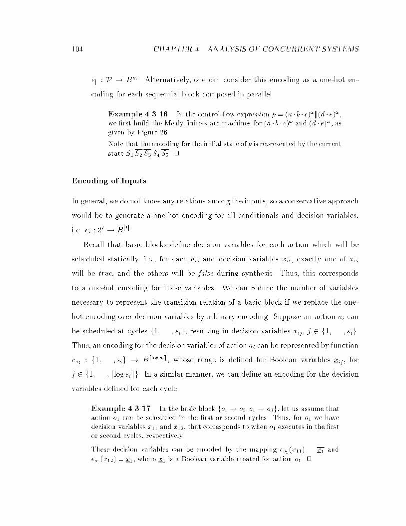
104 CHAPTER 4. ANALYSIS OF CONCURRENT SYSTEMS
ek : P ! Bm. Alternatively, one can consider this encoding as a one-hot en-
coding for each sequential block composed in parallel.
Example 4.3.16. In the control- ow expression p = (a � b � c)!k(d � e)!,
we �rst build the Mealy �nite-state machines for (a � b � c)! and (d � e)!, as
given by Figure 26.
Note that the encoding for the initial state of p is represented by the current
state S1 S2 S3 S4 S5. 2
Encoding of Inputs
In general, we do not know any relations among the inputs, so a conservative approach
would be to generate a one-hot encoding for all conditionals and decision variables,
i.e. ei : 2I ! BjIj.
Recall that basic blocks de�ne decision variables for each action which will be
scheduled statically, i.e., for each ai, and decision variables xij, exactly one of xij
will be true, and the others will be false during synthesis. Thus, this corresponds
to a one-hot encoding for these variables. We can reduce the number of variables
necessary to represent the transition relation of a basic block if we replace the one-
hot encoding over decision variables by a binary encoding. Suppose an action ai can
be scheduled at cycles f1; . . . ; sig, resulting in decision variables xij, j 2 f1; . . . ; sig.
Thus, an encoding for the decision variables of action ai can be represented by function
eai : f1; . . . ; sig ! Bdlog sie, whose range is de�ned for Boolean variables xij, for
j 2 f1; . . . ; dlog sieg. In a similar manner, we can de�ne an encoding for the decision
variables de�ned for each cycle.
Example 4.3.17. In the basic block fo1 ! o2; o1 ! o3g, let us assume that
action o1 can be scheduled in the �rst or second cycles. Thus, for o1 we have
decision variables x11 and x12, that corresponds to when o1 executes in the �rst
or second cycles, respectively.
These decision variables can be encoded by the mapping eo1(x11) = x1 and
eo1(x12) = x1, where x1 is a Boolean variable created for action o1. 2

4.3. REPRESENTATION OF CFFSM AS A TRANSITION RELATION 105
Representing the Output Function
Note that the output function for the �nite-state Mealy machine is represented by
the function � : Q � 2I ! 2O, i.e., for each transition, � represents which outputs
will be generated. We use here a modi�ed representation for the � function. Instead
of representing the possible actions that can be generated for each transition, we
represent which transitions generate a given output.
De�nition 4.15 Let o 2 O be an output of M = (Q; I;O; �; �; q0). An action activa-
tion function Af : O ! Bn �Bm ! B is a Boolean function de�ned for each output
representing the transitions in which the output will be generated.
We can write the action activation function for an output o in the following way.
Af(o) = feq(q) ei(i) such that q 2 Q; i 2 2I and o 2 �(q; i)g.
Example 4.3.18. In the CFE of Example 4.3.15, we have the following
action activation functions for actions a, b and c.
Af (a) = S1 S2 S3
Af (b) = S1 S2 S3
Af (c) = S1 S2 S3
2
Exception Handling in the Transition Relation
Because we partitioned the computation of the �nite-state machine at parallel blocks,
we must take into account when the disable construct crosses the partitioned blocks.
Thus, for each sub-expression pi of a CFE p, we de�ne an input called kill which
forces the CFE to quit its execution, i.e. the CFE pi has an associated input killi
which guards the every transition of pi's FSM by killi. In a disable construct, if pi is
a n-uplink of �(n; p) in p, then executing this command forces the killi input of pi to
be activated.

106 CHAPTER 4. ANALYSIS OF CONCURRENT SYSTEMS
kill
a
b
dc1: ζ
c
c1: 0
a
b
dc1: ζ
c
c1: 0
d
kill :
:
kill
(a) (b)
Q1
Q2
Q3
Q4
Q5
kill
Figure 27: Exception Handling in CFFSMs
Example 4.3.19. In order to construct the CFFSM for the CFE (a � b � (c1 :
�(2; p) � c+ c1 : 0) � d)! � (a � b � (c1 : �(d � p) � c+ c1 : 0) �d)
!, let us �rst consider
the CFFSM for the CFE (a � b � (c1 : 0 � c + c1 : 0) � d)!, which is represented
in Figure 27 (a). We labeled the states of this �gure as states Q1,Q2,Q3,Q4
and Q5, as it can be seen in the �gure. Since the alternative composition
(c1 : �(2; p) � c + c1 : 0) is aborted when � is executed, we create a signal kill
that becomes true when � is executed.
Since we abort the execution of the CFFSM at state Q3 if c1 is true, signal
kill will be assigned the truth value e(Q3) c1, where e(Q3) is the encoding for
state Q3. This signal will guard the execution of every path of the alternative
composition until the CFE executes d � p, as it can be seen in Figure 27 (b).
Note that by setting kill to this value, state Q4 is no longer reachable from the
initial state. 2
Putting it All Together: Computing the Transition Relation
The algorithm of Figure 28 computes the transition relation using the encoding
algorithms presented in this section. We have to distinguish between three types of
CFEs: basic blocks, parallel composition, and sequential composition for encoding
purposes. Collect kill collects all the transitions leading to the cfe coming from a
disable construct. The �nal transition tf1 � . . . � tfn generates a synchronizer that
waits until all transitions tfi have occurred.

4.3. REPRESENTATION OF CFFSM AS A TRANSITION RELATION 107
=� Computing Transition Relation of CFE �=
procedure Compute Tr
f
input: cfe,storage,kill
output: T,�nal transition,reset
if (cfe is basic block) f
return Compute Tr bb(cfe,kill)
g else if (cfe = p1k . . .kpn) f =� Compute Tr of each pi separately �=
killk = collect kill(cfe) _ kill
(Ti; tfi; reseti) = Compute Tr(pi; storage; killk)
T = T1 . . .Tnreset = reset1 . . .resetntf = tf1 � . . .� tf
n
return (T; tf; reset)
g else if (cfe = �(n; p)) f =� Make the leading transition to reset n-uplink block �=
Let p0 be the n-uplink of �(n; p)
collect kill(p0) = collect kill(p0) [ transition leading to �
g else f
killcfe = collect kill(cfe) _ kill
Compute (T; tf; reset) using derivatives
return (T; tf; reset)
g
g
Figure 28: Algorithm to Compute Transition Relation of a CFE
4.3.3 Computing Reachable States and Valid Transitions
We conclude this chapter by showing how we can use the transition relation to com-
pute the set of valid transitions and reachable states.
The algorithm of Figure 29, which is similar to the algorithm presented in [TSL+90,
CHJ+90, CM90], computes the set of reachable states in a CFFSM. In this algorithm,
S0 denotes the encoding for the initial state q0 of M , and XS = Xs[(S1; . . . ; Sn)
(s1; . . . ; sn)] denotes a new characteristic function XS in which every occurrence of si
was replaced by Si. This corresponds to the simulation of a clock tick if we consider
the pair (Si; si) to represent a D- ip op.
In order to compute valid transitions, let us extend the action activation function
Af to a set of actions. We consider T to be the transition relation of a CFFSM in

108 CHAPTER 4. ANALYSIS OF CONCURRENT SYSTEMS
=� Computing Reachable States in the CFFSM �=
procedure Reachable States
f
input: T, S0output: reachable
reachable = S0 =� Initial states are reachable �=
S = S0while (S 6= ;) f
Xs = 9S9c(T (s; c; S)XS =� Find next states satisfying T and XS �=
XS = Xs[(S1; . . . ; Sn) (s1; . . . ; sn)] =� Simulate a clock transition �=
S = S � reachable
reachable = reachable [ S =� Collect next reachable states �=
g
g
Figure 29: Algorithm to Compute Reachable States of a CFFSM
the following de�nitions.
De�nition 4.16 Let A = fa1; . . . ; amg be a set of actions. Then, the action activa-
tion function over set A is de�ned as Af (A) =_
aj2Ai
Af(aj).
Theorem 4.6 Let fA1; . . . ; Akg 2 ALWAYS. A valid transition exists only in
T (^
1�i�k
Af (Ai)j^
1�i�k
Af (Ai))
.
Proof: This follows from the de�nition of fA1; . . . ; Akg 2 ALWAYS and
from Af(Ai). ]
Theorem 4.7 Let fA1; . . . ; Akg 2 NEVER. A valid transition exists only in
T (_
1�i�k
Af(Ai))
.
Proof: This follows from the de�nition of fA1; . . . ; Akg 2 NEVER and
from Af(Ai). ]
4.4. SUMMARY 109
4.4 Summary
In this chapter we showed how to represent a CFE as a Mealy �nite-state machine
by computing the derivatives of the CFE. Derivatives correspond to a cycle by cy-
cle simulation of the CFE. We �rst showed how to compute the derivatives for the
control- ow expressions de�ned in Section 2.2. Then, we presented a more general
de�nition of derivatives for extended control- ow expressions that considered basic
blocks, exception handling and register variables. Because of registers, the state of a
control- ow expressions computed by a derivative had to consider the possible values
of register variables, which were captured by stores and derived stores.
Analysis was performed at the �nite-state machine level, where the unreachable
states violating synchronization constraints were eliminated. We showed that if the
resulting machine is empty, then the speci�cation and its constraints cannot be sat-
is�ed.
For e�ciency, we showed how to represent the �nite-state machine by a transition
relation, and we argued that an e�cient encoding technique should be used in order
to control the number of variables necessary to represent the transition relation.
Chapter 5
Synthesis of Control-Units
In this chapter, we show how to generate control-units from a CFFSM satisfying
design constraints while optimizing some design goal. Since we previously encoded
the possible control-unit implementations by decision variables, design constraints
will be translated into constraints on the possible values these decision variables may
have, and a feasible control-unit will be determined by assigning values to the decision
variables.
We will be considering two types of assignments for decision variables: the assign-
ment of constant values (0 or 1) to decision variables, and the assignment of Boolean
functions over states and conditionals. We will call the former assignment static
scheduling and the latter dynamic scheduling. While static scheduling will be used
to schedule operations in basic blocks (subject to constraints crossing basic blocks),
dynamic scheduling will be used to synthesize the synchronization skeletons for more
complex and loosely coupled interactions among the di�erent parts of a concurrent
description.
In the next section, we formulate the problem of synthesizing control-units from
CFFSMs and we highlight the similarities between static scheduling and dynamic
scheduling. Then, in Section 5.2, we review the techniques for static scheduling
110

5.1. OBTAINING CONTROL-UNITS FROM THE CFFSM 111
of operations in basic blocks subject to timing and resource constraints, and in Sec-
tion 5.3, we show how we can extend these techniques to statically schedule operations
in the basic blocks of a CFE. In Section 5.4, we show how to dynamically schedule
operations for the loosely coupled parts of the design. Our algorithms will be cast
as Integer Linear Programming (ILP) formulations, and solved by a Binary Decision
Diagram (BDD) solver that we developed.
5.1 Obtaining Control-Units from the CFFSM
In this section, we formulate the problem of obtaining control-unit implementations
from CFFSMs. This formulation will be applicable to both the static and dynamic
scheduling techniques to be developed in the following sections of this chapter.
Figure 30 (a) presents the general methodology used for obtaining control-unit
implementations from a CFE. From the CFE representing the speci�cation and design
constraints, in the previous chapter we obtained a CFFSM with the same behavior
of the CFE.
Because we guarded design choices with decision variables, and in particular,
because we guarded the execution time of actions by decision variables, the CFFSM
contains the possible execution ows for the actions of the CFE. Thus, in order to
obtain a feasible control-unit implementation for the concurrent parts of the CFE,
we have to obtain an assignment for the decision variables of the CFE.
If we only consider static assignments to the decision variables, we obtain schedules
for the actions in the CFFSM that do not change with the di�erent states of the
CFFSM. For example, the schedule of an operation relative to the beginning of a
basic block will have a �xed number of cycles under all conditions of the system. As
we mentioned before, these assignments are called static schedules.
We also consider the assignment of Boolean functions (over the transitions of the

112 CHAPTER 5. SYNTHESIS OF CONTROL-UNITS
c
a
x
Integer Linear Programming x = 0 c 0 c 0 c 0 c ...
Control−Unit Implementation c
a
0 c 0 c 0 c ...
Control−Flow Expressions (a.0) || (0.(c:0)*.a) || ((x:0)*.a)ω ω ω
Control−Flow Finite State Machine
Specification Constraints
(a) (b)
NEVER = {{a},{a}}p =
CFFSM
Figure 30: Methodology for synthesizing control-units
CFFSM) to the decision variables. This is used to satisfy more stringent constraints
and constraints among the loosely coupled parts of the system. These assignments
are called dynamic schedules.
Static scheduling and dynamic scheduling can be considered as restrictions of the
behavior of the CFFSM.We consider in this chapter the CFFSMM = (I;O;Q; �; �; q0),
as de�ned in Section 4.2, where I is the set of inputs, O is the set of outputs, Q is
the set of states, � is the transition function (2I �Q! Q), � is the output function
(2I � Q ! 2O) and q0 2 Q is the initial state. A control-unit implementation will
be the restriction of machine M to the set of assignments obtained for the decision
variables. A formal de�nition of an implementation for M is given below.
5.1. OBTAINING CONTROL-UNITS FROM THE CFFSM 113
De�nition 5.1 Let M be the CFFSM corresponding to some CFE p, and let X be
a set of decision variables, i.e. X � I. We call M 0 an implementation of M if the
following conditions hold.
1. The set of states of M 0 is a subset of the set of states of M .
2. The initial states of M and M 0 are the same.
3. The set of transitions of M 0 is a subset of the set of transitions of M .
4. The set of inputs of M 0 is I �X.
5. If every output o � O is executed in some state of M , it will be executed in
some state of M 0.
Thus, an implementation M 0 = (I 0; O;Q0; �0; �0; q0) will be an implementation of
M = (I;O;Q; �; �; q0) if I0 = I � X, Q0 � Q, �0 � �, �0 � � and 8 o � O;�(o) 6=
; ) �0(o) 6= ;. In addition to these requirements, M 0 must also satisfy additional
constraints that will be imposed by the structure of the original speci�cation. These
additional constraints will vary depending whether we are obtaining static schedules
for actions in basic blocks or dynamic schedules.
Example 5.1.1. In Figure 30 (b), we present the steps used to obtain
control-unit implementations from a CFE p. Starting from a CFE p = (a �
0)!k(0 � (c : 0)� � a)!k((x : 0)� � a)!, and a set of synchronization constraints,
i.e. NEVER = ffag; fagg, we obtain a CFFSM corresponding to p. Then, we
�nd a set of assignments to the decision variables of p over time, i.e. X = fxg
over time by casting the problem as an ILP. As mentioned previously in this
section, the control-unit implementation will be the restriction of the CFFSM
with respect to the assignments to the decision variable over time. 2
In the next section, we will review static scheduling techniques for basic blocks
cast as ILP instances. Then, in the following sections, we present static and dynamic
scheduling techniques for the CFFSM.

114 CHAPTER 5. SYNTHESIS OF CONTROL-UNITS
5.2 Scheduling Operations in Basic Blocks
We review here the basic concepts for the scheduling problem that were originally
de�ned in [HLH91, DGL92, Mic94] for basic blocks.
Let O = fo1; . . . ; ong be a set of operations. We assume that each operation oi has
an associated type type(oi) = k, which indicates what kind of resource the operation
uses.
De�nition 5.2 A scheduling problem is a mapping T : O ! N+ that assigns with
each operation a positive integer denoting the starting time of the operation, relative
to the beginning of the basic block
We denote the execution time for operation oi by ti, i.e., T (oi) = ti. Let fr1; . . . ; rmg
be a set of precedence constraints. For any precedence constraint oi1l! oi2 , the map-
ping T is such that the starting time of operation i2 occurs after the starting time of
operation i1 by at least l cycles. Equivalently, ti2 � ti1 � l.
We are going to model the scheduling problem as an instance of Integer Linear
Programming, which can be represented by following set of equations [Nem88].
minXi
cixi
Ax = b
xi 2 f0; 1g
The solution to an ILP problem is an assignment to variables xi such that they
satisfy the set of constraints Ax = b, while minimizing the cost functionP
i cixi. Here,
we are interested in the formulations in which xi are binary variables, i.e., they can
take 0 or 1 values. This problem has been also referred in the literature as a 0-1
Integer Linear Programming problem.
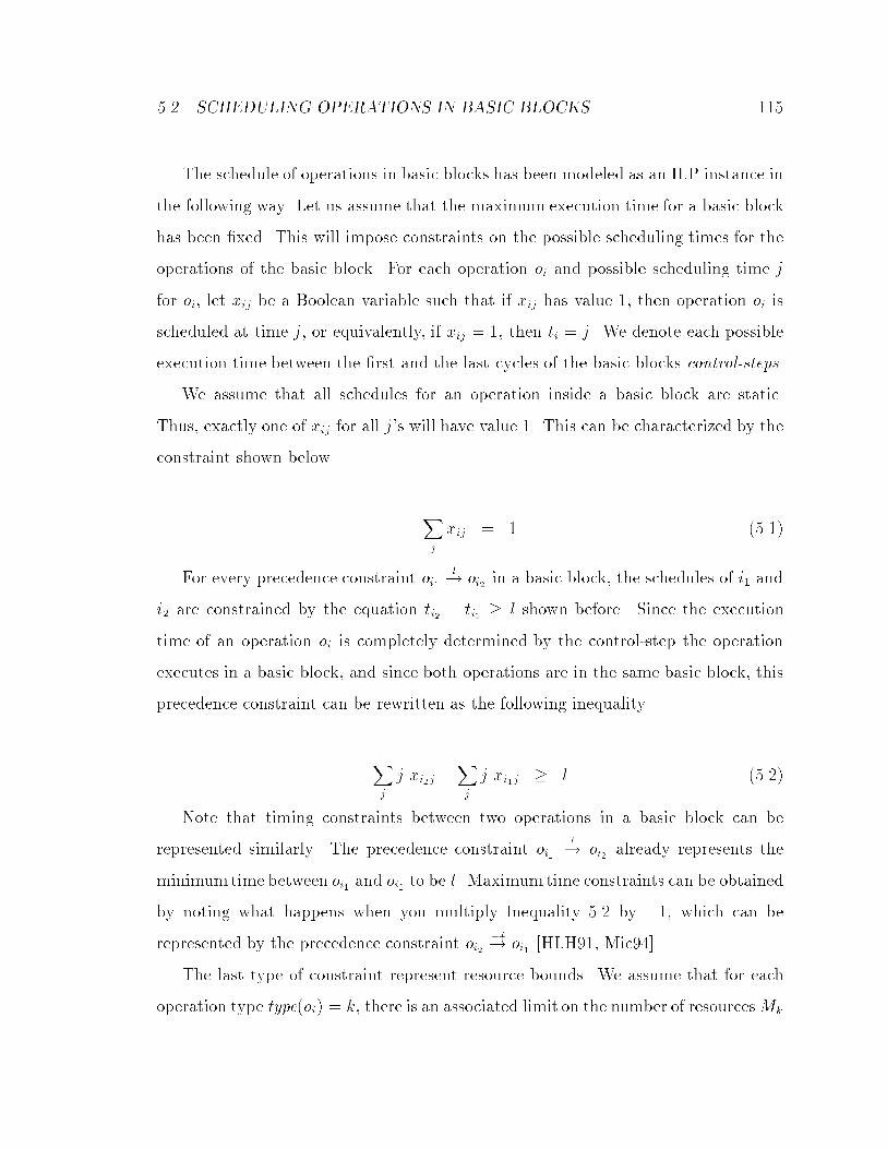
5.2. SCHEDULING OPERATIONS IN BASIC BLOCKS 115
The schedule of operations in basic blocks has been modeled as an ILP instance in
the following way. Let us assume that the maximum execution time for a basic block
has been �xed. This will impose constraints on the possible scheduling times for the
operations of the basic block. For each operation oi and possible scheduling time j
for oi, let xij be a Boolean variable such that if xij has value 1, then operation oi is
scheduled at time j, or equivalently, if xij = 1, then ti = j. We denote each possible
execution time between the �rst and the last cycles of the basic blocks control-steps.
We assume that all schedules for an operation inside a basic block are static.
Thus, exactly one of xij for all j's will have value 1. This can be characterized by the
constraint shown below.
Xj
xij = 1 (5.1)
For every precedence constraint oi1l! oi2 in a basic block, the schedules of i1 and
i2 are constrained by the equation ti2 � ti1 � l shown before. Since the execution
time of an operation oi is completely determined by the control-step the operation
executes in a basic block, and since both operations are in the same basic block, this
precedence constraint can be rewritten as the following inequality.
Xj
j xi2j �Xj
j xi1j � l (5.2)
Note that timing constraints between two operations in a basic block can be
represented similarly. The precedence constraint oi1l! oi2 already represents the
minimumtime between oi1 and oi2 to be l. Maximumtime constraints can be obtained
by noting what happens when you multiply Inequality 5.2 by �1, which can be
represented by the precedence constraint oi2�l! oi1 [HLH91, Mic94].
The last type of constraint represent resource bounds. We assume that for each
operation type type(oi) = k, there is an associated limit on the number of resourcesMk

116 CHAPTER 5. SYNTHESIS OF CONTROL-UNITS
that can be concurrently executing with oi in the basic block. Thus, this constraint
can be represented by the following equation.
Xi such that type(oi)=k
xij � Mk (5.3)
Example 5.2.2. In Figure 17 we presented the possible scheduling times
for a piece of the di�erential equation solver. We represent below the Boolean
variables de�ning the schedule for all operations of the basic block, according
to a maximum execution time of 4 cycles. Operations m1, m2, m3, s1 and s2only require one variable, while operations m4 and m5 require two variables.
xm1;1 = 1
xm2;1 = 1
xm3;2 = 1
xm4;1 + xm4;2 = 1
xm5;2 + xm5;3 = 1
xs1;3 = 1
xs2;4 = 1
2xm3;2 � xm1;1 � 1
2xm3;2 � xm2;1 � 1
3xs1;3 � 2xm3;2 � 1
4xs2;4 � 3xs1;3 � 1
(2xm5;2 + 3xm5;3)� (1xm4;1 + 2xm4;2) � 1
4xs2;4 � (2xm5;2 + 3xm5;3) � 1
In addition to these constraints, if we restrict the number of multipliers to 2,
then we obtain the following additional constraints.
xm1;1 + xm2;1 + xm4;1 � 2
xm3;2 + xm4;2 + xm5;2 � 2
xm5;3 � 2
2

5.2. SCHEDULING OPERATIONS IN BASIC BLOCKS 117
The Integer Linear Programming formulation presented above presumes the exis-
tence of an objective goal that needs to be minimized. In the scheduling problem, the
minimization of the execution time of the basic block and the minimization of some
resource usage costs have been used in the past.
The minimization of execution time can be represented by computing the execu-
tion time of the last operation of the basic block. Let oi be the last operation of the
basic block, or a sink vertex for a basic block, if the basic block does not have a single
last operation, and let its possible schedules be determined by imin and imax. Then,
the cost functionP
j2[imin;imax]j xij represents the cost function that characterizes the
execution time of the basic block, since the sink vertex of the basic block is the last
operation that is executed.
We can also obtain an objective cost function that minimizes a resource cost. For
each resource type k, let ck be its cost. Then the cost functionP
k ckMk denotes the
cost of the basic block in terms of its resources. Note that in this case, Mk is not
assumed to be a constant value, as presented in Inequality 5.3, but a variable that
may take any integer value.
Example 5.2.3. For the set of equations presented in Example 5.2.2, the
minimization of the execution time in the basic block is represented by a cost
function that computes when operation s2 executes. Thus, the cost function is
min 4xs2;4.
If the objective goal is the minimization of resource cost, we replace the last 3
equations of Example 5.2.2 by the following equations.
xm1;1 + xm2;1 + xm4;1 � Mm
xm3;2 + xm4;2 + xm5;2 � Mm
xm5;3 � Mm
In this case, Mm is a variable taking integer values. If we assume that the cost
of a multiplier is cm, the cost function can be represented by min cmMm. 2

118 CHAPTER 5. SYNTHESIS OF CONTROL-UNITS
More recent advances in exact scheduling techniques for basic blocks can be found
in [RB93, Geb91]. We will postpone any discussions until Section 5.5, when we
compare these methods with the methods proposed in this chapter.
5.3 Static Scheduling Operations in CFFSMs
One of the problems with the scheduling formulation presented in the previous sec-
tion is that they can only solve the scheduling problem for basic blocks, and that cost
functions, timing and resource constraints can only be applied to basic blocks. In this
section, we present a methodology for incorporating design constraints and applying
cost functions to the CFFSM, such that an optimal solution can be found that stati-
cally satis�es the design constraints, over a number of basic blocks simultaneously.
Recently, [TWL95] proposed a methodology of Behavior Finite State Machines
(BFSMs) for representing sequential and conditional basic blocks (which are called
behavioral states). In [YW], an algorithm was presented for the scheduling operation
in BFSMs that allowed the satisfaction of timing constraints that crossed behavioral
states. However, these techniques were restricted to sequential and conditional blocks,
and constraints were limited to path-activated timing constraints.
The formulation for the scheduling problem presented in this section considers not
only sequential and conditional paths, as in the case of BFSMs, but also concurrent
blocks. In addition to that, we allow the incorporation of resource constraints, and
the speci�cation of environment processes. Our objective is the derivation of Integer
Linear Programming constraints from the CFFSM, their solution and application
back to the CFFSM.
Because in static scheduling the constraints have to satisfy all the execution con-
ditions of the system modeled by the CFE, we will not consider them to be part of
the systemmodeled by the CFE, but we will extract static scheduling conditions from

5.3. STATIC SCHEDULING OPERATIONS IN CFFSMS 119
the CFFSM instead, and represent them separately.
5.3.1 Extracting Constraints from the CFFSM
We present in this section how we can represent static scheduling constraints of a
CFE. Let M = (Q; I;O; �; �; q0) be a CFFSM corresponding to a CFE p, let T be its
transition relation, and Df be the set of basic blocks of p. For each basic block d 2 Df ,
we assume the actions Ad = fa1; . . . ; ang are the actions de�ned in the precedence
constraints of d, and A0 =[
d2Df
Ad is the set of actions de�ned in all basic blocks of p.
Recall that in the scheduling problem presented in Section 5.2, we de�ned three
types of constraints for the Integer Linear Programming formulation. Equation 5.1
required that only one schedule for each operation was allowed. Inequality 5.2 de�ned
the precedence constraints between two operations. Inequality 5.3 de�ned resource
usage constraints inside a basic block.
In a CFE and its corresponding CFFSM, Equations 5.1 and 5.2 can be obtained
directly from the precedence constraints of a basic block, and the possible scheduling
times for the actions.
Let ai 2 A0 be an action, let j range over the possible scheduling times for ai,
and let xij be a decision variable de�ned for ai. Recall that we represented the
CFFSM by a transition relation in Chapter 4. In that chapter, we also used a e�cient
encoding e(xij) for the decision variables xij. For example, if an action ai could only
be executed in the �rst or second control-steps of a basic block, which corresponds to
de�ning decision variables xi1 and xi2, respectively, then a suitable encoding for the
decision variables of ai would be e(xi1) = xi and e(xi2) = xi, where xi is a Boolean
variable.
Since obtaining only one schedule for an action ai is equivalent to allowing only
one of the encodings for xij to be valid, we can modify Equation 5.1 to the equation

120 CHAPTER 5. SYNTHESIS OF CONTROL-UNITS
below, where e overloads the encoding function e(xij) and an arithmetic function
whose weight is 1 if the encoding e(xij) is evaluated to true, and 0 otherwise.
Xj
e(xij) = 1 (5.4)
Example 5.3.4. Suppose an operation o1 can be scheduled in cycles 1
and 2, resulting in the decision variables x11 and x12. As discussed earlier, each
decision variable will have a corresponding encoding e(x11) and e(x12). Assume
e(x11) = xa and e(x12) = xb. Then the constraint e(x11) + e(x12) = 1 can be
rewritten as the arithmetic formula.
(1 xa + 0 xa) + (1 xb + 0 xb) = 1
It should be clear that this arithmetic function has value 1 if either xaxb or
xaxb. 2
If ai1l! ai2 is a precedence constraint of a basic block, we can only allow the
assignments to the corresponding decision variables of ai1 and ai2 (xi1j and xi2j,
respectively) such that ti2 � ti1 � l, which can be represented in a form similar to
Inequality 5.2.
Xj
j e(xi2j)�Xj
j e(xi1j) � l (5.5)
Note that the function e in these set of ILP constraints acts as a linear transfor-
mation (e(c1f(x)+c2g(x)) = c1e(f(x))+c2e(g(x))) since it is a bijective function and
it distributes over arithmetic addition and multiplication by constants. Consequently,
Inequality 5.3 could be easily rewritten as:
Xi such that type(oi)=k
e(xij) � Mk (5.6)

5.3. STATIC SCHEDULING OPERATIONS IN CFFSMS 121
When the encoding function e is applied to the set of Inequalities 5.1, 5.2, 5.3, we
can no longer use conventional ILP solvers, because the equations are no longer linear
in terms of the new Boolean variables. We show later in this chapter that BDDs can
be used to e�ciently solve these set of equations.
So far, we have shown how we could represent constraints that are limited to basic
blocks. Recall that in Chapter 3 we de�ned statically satis�able constraints, namely
path-activated constraints, resource limiting constraints, and environment processes.
These constraints impose additional restrictions to the decision variables, but they
are not limited to basic blocks. We show in the sequel how to constraint the decision
variables across basic blocks based on these of constraints.
Path-Activated Constraints
In Section 3.2.2, we de�ned a path-activated constraint as a convenience for rep-
resenting timing constraints. Recall that a path-activated constraint is de�ned as
type(n; [l1; . . . ; lm]), where type is one of min, max or delay, and the term li is
either a set of actions or a Boolean guard de�ned over conditionals or comparisons
on registers. We present in this section how we can constrain decision variables in
terms of these path-activated constraints.
In order to constrain the decision variables of a CFE from a path-activated con-
straint, we have to identify how many cycles occur in the CFFSM between two consec-
utive terms li and li+1. Recall that if li and li+1 are actions, then the action activation
functions Af (li) and Af(li+1) will determine in which transitions of the CFFSM the
actions li and li+1 occur, respectively. Thus, we can constrain the decision variables by
counting the number of cycles when we traverse the CFFSM from Af(li) to Af(li+1),
while keeping the decision variables in the traversal.
Since the terms of path-activated constraints include sets of actions and Boolean
guards, we have to extend the action activation function Af for these elements. We

122 CHAPTER 5. SYNTHESIS OF CONTROL-UNITS
call here such extension an activation function, and it will be denoted by A�f . When
applied to a set of actions, A�f will uniquely identify each action activation function.
When applied to Boolean guards, however, A�f indicates in which transitions of the
CFFSM the Boolean guard occurs. In this case, the activation function consists of
two parts, the Boolean guard itself, and the intersection of the transitions for each
conditional or register speci�ed in the Boolean formula of li. We assume in the
following de�nition that the function Cf : G ! Q� 2I returns the set of transitions
in which the Boolean formula guards the transition of the corresponding CFE.
De�nition 5.3
A�f(li) =
_aj2li
xjAf(aj) if li is set of actions f. . . ; aj; . . .g
= Af (a) if li is action a
= gCf (g) if li is Boolean guard g
Note that in the case where li = f. . . ; aj; . . .g, we created a new Boolean variable
xj for each action aj. We call the set of Boolean variables xj by B. This variable
allows us to uniquely identify an action activation function in A�f .
Example 5.3.5. Let p = (fa1 ! a2; a1! a3; a2 ! a4; a3 ! a4g � (c : fb1 !
b2; b1! b3; b2! b4; b3! b4g)�)!, represented graphically in Figure 31 (a), and
let both basic blocks to execute in at most 4 cycles. The CFFSM is presented
in Figure 31 (b), where eta4 corresponds to the condition when the �rst basic
block requires 4 cycles to execute, and etb4 corresponds to the condition when
the second basic block requires 4 cycles to execute.
Because operations a4 and b4 can only execute in the third or fourth cycles
of their respective basic blocks, we can consider the exit conditions for the
basic blocks in the �rst, second and third cycles to be always false, since all
operations of the basic block must execute, according to our de�nition of an
implementation for a CFFSM. In addition to that, the exit condition for the
fourth cycle is always true, because after executing the fourth cycle of the basic
block, the basic block must exit.
Note also that a1 and b1 can execute in the �rst or second cycles of their
respective basic blocks, a2, a3, b2 and b3 can execute in the second or third

5.3. STATIC SCHEDULING OPERATIONS IN CFFSMS 123
S0 S1 S2
S0 S1 S2
S0 S1 S2
S3 S4 S5
S3 S4 S5
S3 S4 S5
c
c
c
cc
c
c c
et a4et a4
et a4
et b4 et b4
et b4
c
c
a1
a2 a3
a4
b1
b2 b3
b4
c
(a) (b)
Figure 31: (a) Graphical representation of CFE p and (b) CFFSM for p
cycles of their respective basic blocks and a4 and b4 can execute in the third or
fourth cycles of their respective basic blocks.
The Boolean formulae de�ning the execution time for the basic blocks are pre-
sented below, where ya4 and yb4 represent decision variables created for the
fourth cycles of the �rst and second basic blocks, respectively.
eta4 = (e(xa44) _ e(ya4))
etb4 = (e(xb44) _ e(yb4))
The following are activation functions for the CFFSM presented in the �gure.
A�f (a1) = e(xa11)(S0 S1 S2) _ e(xa12)(S0 S1 S2)
A�f (c) = c(S0 S1 S2 eta4 _ S0 S1S2 _ S3 S4 S5 etb4 _ S3 S4S5)
2
The extraction of a path-activated constraint can be easily explained now. The
idea is that we traverse the CFFSM represented by a transition relation T starting
at A�f(l1), then waiting until A�
f (l2) occurs in the traversal, then waiting for A�f(l3),

124 CHAPTER 5. SYNTHESIS OF CONTROL-UNITS
Af (l1)
Af (l1)
Af (l2)
Af (l2) Af (lm−1 )
Af (lm−1 )
Af (lm )
Af (lm )
SF
*
* *
* *
* *
*
Figure 32: Finite-State Machine Representing the Path-Activated Constraint
and proceeding until we reach A�f(lm). Instead of existentially quantifying all in-
puts of the CFFSM during the traversal, as shown in the algorithm of Figure 29,
we keep the decision variables such that at the end we have the set of valid assign-
ments for the decision variables. The traversal of the path-activated constraint can
be represented by the �nite-state machine of Figure 32. We traverse the CFFSM
and the machine represented in Figure 32 until we reach state SF . If the path con-
straint is min(n; [l1; . . . ; lm]), then we only keep the assignments to the decision vari-
ables for which SF is reached in more than n � 1 cycles. If the path constraint is
max(n; [l1; . . . ; lm]), then we only keep the assignments to the decision variables if SF
is reached during the traversal of the CFFSM in less than n + 1 cycles. If the path
constraint is delay(n; [l1; . . . ; lm]), then we only keep the assignments to the decision
variables in which SF is reached during the traversal in exactly n cycles.
Before we present the algorithms for computing the minimumand maximumpath-
activated constraints, let us show �rst that this procedure is equivalent to Inequal-
ity 5.5 when two actions are speci�ed in the same basic block.
Theorem 5.1 If a1 and a2 belong to the same basic block, then min(n; [a1; a2]) =Pj jx2j �
Pj jx1j � n.
Proof: First note that A�f(a1) =
Wj e(x1j)F
1
j (c; S), for some function
F 1
j (c; S). Thus, we can consider in this representation of A�f(a1) that
F 1
j (c; S) carries the information about the execution time for a1, while
e(x1j) carries the decision on whether a1 will be executed at transition
F 1
j (c; S) or not. SinceP
j e(x1j) = 1, thenWj e(x1j)F
1
j (c; S) =P
j e(x1j)
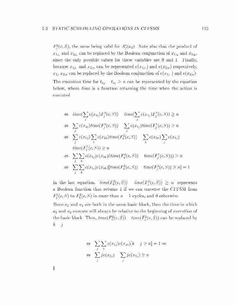
5.3. STATIC SCHEDULING OPERATIONS IN CFFSMS 125
F 1
j (c; S), the same being valid for A�f(a2). Note also that the product of
x1j1 and x2j2 can be replaced by the Boolean conjunction of x1j1 and x2j2,
since the only possible values for these variables are 0 and 1. Finally,
because x1j1 and x2j2 can be represented e(x1j1) and e(x2j2) respectively,
x1j1x2j2 can be replaced by the Boolean conjunction of e(x1j1) and e(x2j2).
The execution time for ta2 � ta1 � n can be represented by the equation
below, where time is a function returning the time when the action is
executed.
, time(Xj
e(x2j)F2
j (c; S))� time(Xj
e(x1j)F1
j (c; S)) � n
,Xj
e(x2j)time(F2
j (c; S))�Xj
e(x1j)time(F1
j (c; S)) � n
,Xj
e(x1j)Xk
e(x2k)time(F2
k (c; S))�Xk
e(x2k)Xj
e(x1j)
time(F 1
j (c; S)) � n
,Xj
Xk
e(x1j)e(x2k)(time(F2
k (c; S))� time(F 1
j (c; S))) � n
,Xj
Xk
e(x1j)e(x2k)[time(F2
k (c; S))� time(F 1
j (c; S)) � n] = 1
In the last equation, [time(F 2
k (c; S)) � time(F 1
j (c; S)) � n] represents
a Boolean function that returns 1 if we can traverse the CFFSM from
F 1
j (c; S) to F2
k (c; S) in more than n� 1 cycles, and 0 otherwise.
Since a2 and a1 are both in the same basic block, then the time in which
a1 and a2 execute will always be relative to the beginning of execution of
the basic block. Thus, time(F 2
k (c; S))� time(F 1
j (c; S)) can be replaced by
k � j.
,Xj
Xk
e(x1j)e(x2k)[k � j � n] = 1)
,Xj
je(x2j)�Xj
je(x1j) � n
]

126 CHAPTER 5. SYNTHESIS OF CONTROL-UNITS
We can now present a corollary to the theorem above that provides the tool for
computing the minimum and maximum path-activated constraints. Function Time
represents the number of cycles to traverse A�f(l1) to A�
f(lm), when passing through
A�f(l2); . . . ; A
�f(lm�1). Note that when constraining the decision variables with respect
to a path-activated constraint, all the actions that can be scheduled in the path will
be constrained. We denote by a1, . . . , ao the set of actions that are executed by the
CFE while executing the thread [l1; . . . ; lm], and we denote by x1j1, . . . , xojo their
respective decision variables, where j1, . . . , jo range over the set of possible cycles
where action ai can be scheduled. When computing the constraint for the minimum
and maximumthread execution time, we must exclude the assignments to the decision
variables which invalidates the limit on execution time for the thread. More formally,
Corollary 5.1 min(n; l1 . . . lm) =Xj1
Xj2
. . .Xjo
^i
e(xiji)[Time(A�f(l1); . . . ;
A�f(lm)) � n] = 1, where actions a1; . . . ; ao are the actions whose decision variables
x1j1; . . . ; xojo become constrained when traversing l1; . . . ; lm for more than n�1 cycles.
Corollary 5.2 max(n; l1 . . . lm) =Xj1
Xj2
. . .Xjo
^i
e(xiji)[Time(A�f(l1); . . . ;
A�f(lm)) � n] = 1, where actions a1; . . . ; ao are the actions whose decision variables
x1j1; . . . ; xojo become constrained when traversing l1; . . . ; lm for less than n+1 cycles.
Figure 33 presents the algorithm for minimum path-activated constraint and Fig-
ure 34 presents the algorithm for maximumpath-activated constraint. The algorithm
for exact delay is not presented, since it can be easily derived from both of these algo-
rithms, and it corresponds to the intersection of the constraints obtained for minimum
and maximum path constraints.
In Figures 33 and 34, we traverse the �nite-state machine presented in Figure 32
while traversing the transition relation T . For each state i of the �nite-state machine
of Figure 32, we keep the current transitions of the CFFSM leading to i in variable

5.3. STATIC SCHEDULING OPERATIONS IN CFFSMS 127
=� Computing Minimum Path-Activated Constraint from CFFSM �=
procedure Minimum Path Activated Constraint
f
input: T, A�f(l1); . . . ; A
�f(lm), n, Valid
output: constr
T1 = A�f(l1)
for(i = 1; i � m; i+ +) f
Ti+1 = Ti A�f(li+1)
Ti = Ti A�f(li+1) Valid
g
=� traverse transition relation only n� 1 times �=
for(timer = n� 1; timer > 0; timer� �) f
for(i = 1; i < m; i ++) f
=� Advance clock tick for Ti �=
Ti = 9conditionals TiF = Ti=� propagate F as far as possible �=
for(j = i; F 6= 0 && j � m; j ++) f
NTj = NTj _F A�f(lj) Valid
F = F A�f(lj) Valid
g
if (j == m + 1) constr = constr _ F
g
8i NTi = Tig
constr = 8B(9S constr)
g
Figure 33: Algorithm to Compute a Minimum Path-Activated Constraint in a
CFFSM
Ti. Since the CFFSM may make multiple transitions at the same time when A�f(li)
and A�f(li+1) are satis�ed simultaneously, after computing a new Ti (represented by
NTi), we must propagate it as far as possible, or until this new transition can not be
propagated any longer in the machine of Figure 32.
In the case of a minimum path-activated constraint, we compute the relations
among decision variables when the machine is traversed in less than n + 1 cycles,
since these assignments will be invalid. For the case of a maximum path-activated
constraint, we consider that only these assignments will be valid assignments. In

128 CHAPTER 5. SYNTHESIS OF CONTROL-UNITS
=� Computing Maximum Path-Activated Constraint from CFFSM �=
procedure Maximum Path Activated Constraint
f
input: T, A�f(l1); . . . ; A
�f(lm), n, Valid
output: constr
T1 = A�f(l1)
for(i = 1; i � m; i ++) f
Ti+1 = Ti A�f(li+1)
Ti = Ti A�f(li+1) Valid
g
=� traverse transition relation only n times �=
for(timer = n� 1; timer � 0; timer� �) f
for(i = 1; i < m; i ++) f
=� Advance clock tick for Ti �=
Ti = 9conditionals TiF = Ti=� propagate F as far as possible �=
for(j = i; F 6= 0 && j � m; j + +) f
NTj = NTj _ F A�f(lj) Valid
F = F A�f(lj) Valid
g
if (j == m + 1) constr = constr _ F
g
8i NTi = Tig
constr = 8B 9S constr
g
Figure 34: Algorithm to Compute a Maximum Path-Activated Constraint in a
CFFSM
that way, each computation of a path-activated constraint can be computed in a
�nite number of traversals (O(m2n)). The universal quanti�cation of the Boolean
variables in B guarantees that the constraints on the decision variables will satisfy
all assignments to the decision variables that can be constrained from each action of
li. Finally, because complementing a set of states can generate a state which is not
valid, every time we complement a set of states we intersect it with the variable Valid,
which represents the set of reachable states of the CFFSM.
Example 5.3.6. A minimum execution time of 2 cycles between a1 and c
can be computed as follows. Let e(xa11) = xa1 and e(xa12) = xa1 . Thus, the

5.3. STATIC SCHEDULING OPERATIONS IN CFFSMS 129
SF
*
* *
*
Af (a 1)
Af (a 1)
Af (c)
Af (c)
1 2
Figure 35: Path-Activated Constraint FSM for min (2; [a1; c])
following activation functions were computed in Example 5.
A�f (a1) = xa1(S0 S1 S2) _ xa1(S0 S1 S2)
A�f (c) = c(S0 S1 S2 eta4 _ S0 S1S2 _ S3 S4 S5 etb4 _ S3 S4S5)
As described in the algorithm of Figure 33, we traverse the machine of Figure 35,
which is the machine describing the path-activated constraint min (2; [a1; c]).
We begin the traversal of the transition relation from A�f (a1), i.e., from the
transition xa1(S0S1 S2)_xa1(S0 S1 S2). Thus, considering A�f (a1) as the initial
transition, the machine of Figure 35 steps to state 2. After the �rst transition
of T , the set of reachable states of T becomes xa1(S0 S1 S2) _ xa1(S0 S1 S2).
Since this new state intersects A�f (c), when xa1 is true, the machine of Figure 35
makes a transition from state 2 to state SF when xa1 is true.
No additional transitions are required for the path-activated constraint, and
xa1etb4S0S1S2 is the only transition that violates the path-activated constraint.
After quantifying out the state and conditional variables of the constraint, we
obtain the constraint xa1 etb4 = xa1 e(xa44) e(ya4), which is the only condition
that violates the path-activated constraint. 2
Resource Usage Constraints
We present in this section how we can generalize Inequality 5.6 to CFFSMs, in a
manner similar to the extensions described for path-activated constraints. The basic
idea is to use the transitions to detect any possibility of con ict in a set of actions,
and then quantifying out all variables of the transition but the decision variables.
We use the resource limiting constraints that were de�ned in Section 3.2.2, i.e.,
the constraint limit(n; fa1 . . .amg), where n is the maximum number of concurrent
executions of the actions in the set fa1 . . . amg.

130 CHAPTER 5. SYNTHESIS OF CONTROL-UNITS
In order to constrain the decision variables of actions in the set, we have to com-
pute recursively function C(n; a1 . . .am), which returns a Boolean function in which
at least n out of m action activation functions Af(ai) are true.
De�nition 5.4
C(n; ai . . . am) =
8>>>>><>>>>>:
0 if n > m� i+ 1
1 if n = 0
(Af(ai)C(n� 1; ai+1 . . .am)) _ C(n; ai+1 . . .am) otherwise
For e�ciency purposes, we implement C(n; ai . . . am) using a dynamic program-
ming paradigm [CLR90] such that we do not have to recompute C(n; ai+1 . . .am)
every time it is needed.
We can now de�ne limit by the following formula.
De�nition 5.5 limit(n; fa1 . . . amg) = 9 R C(n+ 1; a1 . . . am).
where R = S [ s [ conditionals.
This formula �rst computes the compositions of actions which yield more than
the n available resources. Then, it existentially quanti�es conditional variables, and
present/next state variables of the action activation functions. Finally, the result is
complemented, yielding the constraints on the decision variables such that less than
n of the actions fa1; . . . ; amg are executed concurrently.
Example 5.3.7. In Example 5.2.2, let us assume the constraint
limit (1; fa1; a2; a3; a4g) was speci�ed. Let us also assume that e(xaij) = xaiand e(xaij+1) = xai for a1, a2, a3 and a4.
Thus, the following are the activation functions for a1, a2, a3 and a4.
A�f (a1) = xa1(S0 S1 S2) _ xa1(S0 S1 S2)
A�f (a2) = xa2(S0 S1 S2) _ xa2(S0 S1 S2)
A�f (a3) = xa3(S0 S1 S2) _ xa3(S0 S1 S2)
A�f (a4) = xa4(S0 S1 S2) _ xa4(S0 S1 S2)

5.3. STATIC SCHEDULING OPERATIONS IN CFFSMS 131
According to the Equation presented before, limit(1; fa1; a2; a3; a4g) can be ob-
tained by �rst computing C(2; a1a2a3a4), which is represented by the following
equations.
C(2; a1 a2 a3 a4) = A�f (a1)C(1; a2 a3 a4) _ C(2; a2 a3 a4)
...
= A�f (a1)(A
�f(a2) _A
�f (a3) _ A
�f(a4)) _
A�f (a2)(A
�f(a3) _A
�f (a4)) _ A�
f(a3)A�f(a4)
= (xa1(xa2 _ xa3) _ xa2 xa3)S0 S1 S2 _
(xa2(xa3 _ xa4) _ xa3xa4)S0 S1 S2
After quantifying out state variables and conditionals, we obtain the following
equation:
9S C(2; a1 a2 a3 a4) = (xa1(xa2 _ xa3)_ xa2 xa3) _ (xa2(xa3 _ xa4) _ xa3xa4)
Thus, limit (1; fa1; a2; a3; a4g) = xa1(xa2 xa3 _ xa2 xa3)xa4 . 2
Environment Processes
We show in this section the last type of constraint that is satis�ed statically, namely
environment processes. As de�ned in Section 3.2.2, an environment process is a
process env which is a suitable representation of the environment and is composed in
parallel with a portion of the control- ow expression for the speci�cation p. Because
pkenv must constrain the assignments on decision variables statically, an environment
process must be strongly coupled with the speci�cation p by providing the necessary
synchronization in terms of ALWAYS and NEVER sets.
In this section, we show how we can obtain constraints for the decision variables
from these synchronization sets.
We showed in Section 4.3.3 that if the multiset fA1; . . . ; Akg consisting of the
sets of actions Ai were included in the ALWAYS set, then the set of valid transi-
tions was contained in T (V1�i�k Af(Ai) _
V1�i�k Af(Ai)). Similarly, if the multiset

132 CHAPTER 5. SYNTHESIS OF CONTROL-UNITS
fA1; . . . ; Akg consisting of the sets of actions Ai were included in the NEVER set,
then the set of valid transitions was contained in T (W
1�i�k Af(Ai)).
In order to statically constrain decision variables, we have to extract these rela-
tions from (V
1�i�k Af(Ai) _V1�i�k Af (Ai)) and (
W1�i�k Af(Ai)) by keeping only the
assignments to decision variables. For the ALWAYS case, we should consider the
assignments for the decision variables in which the valid transitions contain either all
the actions of the set executing at the same time or no actions of the set executing
at the same time. For the NEVER case, we should consider only the valid transitions
in which not all the actions in the set are executed at the same time.
De�nition 5.6
always =^
fA1;...;Akg2ALWAYS
9 R (^
1�i�k
Af (Ai) _^
1�i�k
Af(Ai)Valid)
never =^
fA1;...;Akg2NEVER
9 R (Valid_
1�i�k
Af(Ai))
where R = S [ s [ conditionals.
Example 5.3.8. In Example 5.3.5, we can also constrain the decision
variables of p by composing p with an environment process. According to our
assumptions about environment processes, recall that an environment process
must be tightly coupled with p, for example the process env = (a � 0 � 0 � 0 � (c :
0 � 0 � b)�)!, with ALWAYS = fffag; fa1gg; ffbg; fb4ggg.
This environment process not only constrains the delay between a1 and c to be
2 cycles, but it also constrains the execution time for the second basic block
to be 3 cycles. Thus, the constraint resulting from this environment process is
eta4 etb3. 2
5.3.2 Exact Scheduling for Basic Blocks
We presented previously how to extend the constraint formulation for the decision
variables to consider the speci�cation represented by the CFFSM. In this section,

5.3. STATIC SCHEDULING OPERATIONS IN CFFSMS 133
we show how we can use Binary Decision Diagrams to represent the scheduling and
resource usage constraints de�ned in the previous section. Are pointed out before,
because these constraints are represented by mixed Boolean/arithmetic constraints,
a conventional Integer Linear Programming solver will not be e�cient for solving this
set of constraints. Instead, we use a Binary Decision Diagram based solver similar to
the ones described in [RB93, JS93]. However, instead of using a conventional Integer
Linear Programming formulation, our solver can handle a more general formulation,
as described below.
LetX = fx1; . . . ; xmg be a set of Boolean variables, gi and fij be Boolean functions
over X and ci, aij and bj be numeric constants. A mixed Boolean/ILP instance can
be represented by the following set of equations.
minXi
cigi(X)
Xi
aijfij(X) � bj
Note that, in principle, this formulation can be converted into an Integer Linear
Programming formulation by introducing more variables and equations. The original
formulation of the scheduling problem which was represented by Inequalities 5.1,5.2
and 5.3, for example, contains more variables than the equivalent formulation repre-
sented by Inequalities 5.4,5.5 and 5.6.
In Appendix B we present a brief introduction to Binary Decision Diagrams, and
we show how BDDs can be used to represent the Boolean/ILP constraints described
above. The reader should refer to [BRB90, Bry86, Bry92] for a throughout explana-
tion on BDDs, including details of an e�cient implementation [BRB90].

134 CHAPTER 5. SYNTHESIS OF CONTROL-UNITS
Generating Objective Functions
In the general formulation for the Integer Linear Programming problem we presented
in the previous section, we mentioned the objective functionminP
i cigi(X), without
mentioning how to obtain it. We present here a way to generalize the cost functions
to range over decision variables of the CFFSM.
We consider here two type of objective functions, execution time and resource
constraint. We represent objective functions by functional vectors, which are de�ned
below.
De�nition 5.7 A functional vector is the vector f : Bn! Bm in which fi(X) repre-
sents the i-th output bit of f , where X � Bn.
Example 5.3.9. The functional vector
f =
"a _ b
ab
#
corresponds to the Boolean functions f0 = a _ b and f1 = ab. 2
A functional vector f = ff0; . . . ; fmg can be used to represent a mapping fN :
Bn ! N by assuming that each fi spans a partition of the Boolean space Bn, i.e.,
fifj = ; if i 6= j andSi fi = 1. Moreover, for the assignments that satisfy the Boolean
equation fi(X), the mapping fN (X) is assumed to have value i. We call function fN
a numeric extension to the functional vector, and f the functional vector of fN .
We use the notation fN =P
i i fi = 0 f0 + 1 f1 + � � � + m fm to represent the
numeric extension of the functional vector f = ff0; f1; f2; . . . ; fmg of length m + 1.
We suppress the term i fi if fi = 0.
Using this de�nition, we can apply arithmetic operations to functional vectors,
such as addition and multiplication.
De�nition 5.8 Let f and g be two functional vectors of length m1 and m2, respec-
tively, and let fN and gN be their numeric extension.

5.3. STATIC SCHEDULING OPERATIONS IN CFFSMS 135
In the addition of fN and gN , represented by hN = fN +gN , the functional vector
for hN has size m1 +m2 and it satis�es the following relation.
hk(X) =_
i;j : i+j=k
fi(X)gj(X)
In the multiplication of fN and gN , represented by hN = fN � gN , the functional
vector for hN has size m1 �m2 and it satis�es the following relation.
hk(X) =_
i;j : i�j=k
fi(X)gj(X)
Example 5.3.10. Let fN (x1) = 3x1 + 2x1 and gN (x1) = x1 + 4x1, then:
fN (x1) + gN (x1) = 3x1 + 7x1
fN (x1) � gN (x1) = 2x1 + 12x1
2
We can now de�ne the objective function for the execution time of a basic block
d.
De�nition 5.9 etN (d) =P
i i et(d; i).
When composing the cost function for a whole path of the speci�cation, we can
compute the execution time for each basic block, and add the execution times using
the de�nition above for the numeric extension of functional vectors.
Example 5.3.11. In Example 5.2.2, the numeric extension of the functional
vectors denoting the execution time for the �rst and the second basic blocks
are given below.
etN (1) = 4eta4 + 3eta4
etN (2) = 4etb4 + 3etb4

136 CHAPTER 5. SYNTHESIS OF CONTROL-UNITS
The numeric extension of a functional vector denoting the execution time in
the path consisting of the �rst and second basic blocks is given by etN (1) +
etN (2) = 8eta4 etb4 + 7(eta4 etb4jeta4 etb4) + 6eta4 etb4. 2
We can also obtain a cost function for resources, using the constraints for resource
constraints. Let fa1; . . . ; ang be a set of actions and let the cost of each resource be c.
Recall that the function limit(m; fa1; . . . ; ang) computes the set of assignments for
the decision variables such that at most m of the n actions execute at the same time.
We use this function to determine how many actions will be executed concurrently in
the de�nition presented below.
De�nition 5.10 The cost of using resources fa1; . . . ; ang is de�ned as
resourceN (fa1; . . . ; ang) =Xi
(c i)limit(i; fa1; . . . ; ang)^
0�j<i
limit(j; fa1; . . . ; ang)
Example 5.3.12. Assuming the cost of each action ai is 1, the cost function
representing the number of concurrent uses of action ai is shown below.
resourceN (fa1; a2; a3; a4g) = 3(xa1 xa2 xa3 _ xa2 xa3 xa4) +
2((xa1 _ xa4)(xa2 xa3 _ xa2 xa3) _ xa1 xa2 xa3 _
xa2 xa3 xa4) + 1 (xa1(xa2 xa3 _ xa2 xa3)xa4)
2
Solving the Integer Linear Programming Problem
We present now an algorithm for solving the scheduling problem de�ned in the pre-
vious sections.
We split the solution method into two portions: solve and commit. Solve obtains
a set of solutions that satis�es the constraints given by Inequalities 5.4,5.5 and 5.6,
path-activated constraints, resource limiting constraints and environment processes,
while minimizing the objective function given by the numeric extension of a functional
vector.

5.3. STATIC SCHEDULING OPERATIONS IN CFFSMS 137
Commit obtains a unique assignment to the Boolean variables from the set of sat-
isfying assignments obtained by solve. The advantages of such methods are twofold.
First, we can apply solve with respect to several objective functions before commit-
ting to a single solution. For example, the primary goal may be the minimization of
execution time, and the secondary goal may be the minimization of resource usage.
Second, because the complexity of the ILP (and the corresponding BDDs) will be
dependent on the number of variables and in the number of constraints, it may be
worth while to solve some basic blocks �rst in order to reduce the complexity of the
ILP solution for the whole system, but instead of committing to a single solution for
each part of the system being solved, we carry to the other basic blocks the set of
satisfying assignments such that those parts will have more degrees of freedom when
selecting an optimal solution.
Note that solve and commit steps are possible only because we are using a Boolean
representation for the solution space of the ILP problem, since conventional ILP
solvers will only give you a single solution.
The algorithm for solve is presented in Figure 36. We assume that constr is the
conjunction of the constraints obtained previously, and g is a functional vector whose
numeric extension represents a cost function.
procedure Solve
f
input: constr, g
output: X =� set of satisfying assignments �=
foreach (i = 0; i � jgj; i + +) f
X = gi constr
if (X 6= 0) break
g
g
Figure 36: Algorithm to Compute Solve
When committing to a single solution, we have to restrict the behavior of the

138 CHAPTER 5. SYNTHESIS OF CONTROL-UNITS
CFFSM by projecting the assignments of the decision variables back to the CFFSM
M in order to obtain an implementation M 0.
Let X0 be a set of assignments to decision variables which have been resolved
by a commit operation. An implementation with respect to X0 can be obtained by
constraining the output function and the transition functions ofM with respect toX0.
SinceM is represented by the transition relation T and the action activation function
Af(a) for all actions a of M , an implementation M 0 can be obtained by intersecting
T and Af (a) with X0, and then quantifying out the variables of X0. Such operation
has been de�ned by McMillan as an AND-Exists [McM93].
S0 S1 S2
S0 S1 S2
S0 S1 S2
S3 S4 S5
S3 S4 S5
S3 S4 S5
c
c
c
c
Figure 37: Implementation for CFFSM
Example 5.3.13. If we �rst solve the set of constraints using the cost
function min etN (a) + etN (b), followed by solving the set of constraints using
as a secondary goal the minimization on the number of resources ai and bi, we
obtain the implementation of Figure 37.
In this implementation, actions a1 and b1 execute in the �rst transition of
their respective basic blocks, actions a2, a3, b3 and b4 execute in the second
transition of their respective basic blocks and actions a4 and b4 execute in the
third transition of their respective basic blocks. 2

5.4. DYNAMIC SCHEDULING OPERATIONS IN CFFSMS 139
5.4 Dynamic Scheduling Operations in CFFSMs
Searching for static schedules for operations can lead to overconstrained problems if
the concurrent parts are not coupled enough so that a static schedule can be found.
For example, in the synchronization synthesis problem of Example 3.2.9, no static
schedule can be found for the bus accesses of p3 if p1 and p2 are not considered or
the problem becomes overconstrained if p1, p2 and p3 are considered and we attempt
to �nd a static schedule that satis�es the synchronization constraints, because the
accesses to the bus of p2 are non-deterministic, i.e. they depend on the result of the
evaluation of a conditional.
In this section, we will present a technique for generating control-unit implemen-
tations in which operations or basic blocks are synchronized with respect to processes
that may not be tightly coupled. To determine when the operations can execute,
we must consider the ow of control in conditional and concurrent paths to be in-
dependent of each other, as opposed to the procedure for �nding static schedules
presented in the previous section. In such systems, loops make the analysis of the
control- ow to depend on the di�erent assignments to the conditionals. Concurrency
implies that di�erent instances of the same piece of computation require di�erent
decisions. Finally synchronization implies that the di�erent parts of the speci�cation
should not be treated separately. Thus, the complexity of the synthesis task becomes
much higher.
Example 5.4.14. In Example 4.2.13, we represented the CFFSM for the
system consisting of the concurrent processes p1kp2kp3, where p1 = (a � 0)!,
p2 = (0 � (c : 0)� � a)! and p3 = ((x : 0)� � a)!, with the NEVER set being
ffag; fagg.
Recall that in this example, our goal here is the synthesis of a feasible control-
unit for p3 such that no two bus accesses occur at the same time. If we disregard
the interactions of the other concurrent parts of the speci�cation, then we will
not be able to synthesize the control-unit that satis�es the design constraint.
In Figure 24 (b), the CFFSM contains already all possible assignments to the

140 CHAPTER 5. SYNTHESIS OF CONTROL-UNITS
decision variables of the system. Note that there are two possible transitions
from State 1, one to State 0 and another to State 2. The former transition
occurs only if p2 executes the bus access (represented by action a), while the
latter transition only executes if p2 does not make a bus access. Thus, any
assignment to x will have to consider if p2 is accessing the bus or not. 2
We present in the sequel the ILP formulation for the synchronization synthesis
problem. We consider M = (I;O;Q; �; �; q0) to be the CFFSM representing the
behavior of a CFE and M 0 = (I;O;Q0; �0; �0; q0) to be an implementation of M 0, as
de�ned in Section 5.1.
The procedure we will present in this section can be considered as another exten-
sion to the scheduling technique presented before. In the previous section, because
the design constraints were satis�ed for all possible executions of the system, we did
not have to consider the state of the CFFSM, but only decision variables. When
we dynamically schedule the CFFSM, we will have to consider the global state of
the system being synthesized in addition to the decision variables, since the decision
variables will be functions of the transitions of the CFFSM.
In order to obtain an implementationM 0 fromM , we have to identify which states
will be included in M 0 and which transitions will be part of the transition function
for M 0. Thus, we create a Boolean variable yp for each state qp of M . If the Boolean
variable yp is set to 1, our interpretation will be that the state qp will belong to M0.
We will denote the state qp by p in the remainder of this section.
In order to determine a subset of the transitions of M 0, we subdivide each guard f
of a transition �(qp; f) into two conjoined parts. The �rst part contains only decision
variables and the second part contains only conditional variables. Let us call the �rst
part fx and the second part fc. Now, for each state qp, decision variable x of fx and
for each di�erent Boolean formula fc of qp, we create a Boolean variable x(qp;fc). In
the solution of the ILP problem, the variables x(qp;fc) are assigned 0-1 values such
that if fxWx x(qp;fc)
= 1, then �(qp; f) belongs to M 0, i.e., if fx evaluates to 1

5.4. DYNAMIC SCHEDULING OPERATIONS IN CFFSMS 141
when each variable x of fx is assigned the value of x(qp;fc), then �(qp; f) will belong
to M 0.
Let us de�ne also fcx which stands for (8x 2 x)fx(x = xp;fc)jx, i.e., the formula
obtained by replacing every occurrence of x 2 fx by xp;fc. We call a transition in
which fcx = 1 a satisfying transition.
Finally, letX = fxp;fcg[fypg be the set of all Boolean variables de�ned previously
for the �nite-state machine M . We want to obtain an assignment to the variables in
X such that the following set of equations hold.
� The initial state of the �nite-state machine M is a valid state of every imple-
mentation M 0 of M : yp = 1, where p denotes here the original control- ow
expression;
� If a state of M 0 has a satisfying transition to a state p0, then state p0 is also a
state of M 0. More formally, each state p0 of M is a state of M 0 (yp0 = 1) if for
every transition to p0 (�(fxfc; p) = p0), yp0 =Wp ypf
cx.
� For each alternative composition in which the guards are decision variables, only
one decision variable should be true for a given state of the �nite-state machine.
This statement is captured by following formula:Pxp;fc = 1, for all p and
transitions �(p; f) = p0 and �(p; f) = a such that x 2 x.
� For each causality constraint (x : 0)�, where x is a decision variable, we assume
that eventually the computation should proceed. In other words, there is at
least one state of the implementationM 0 in which x should be di�erent from 1.
The following equation captures this constraint:
^�(p;f)=p0^�(p;f)=a
(^xp;fc _ yp) = 0

142 CHAPTER 5. SYNTHESIS OF CONTROL-UNITS
Example 5.4.15. Let us consider the �nite-state machine of Figure 24 for
the synchronization problem presented in Section 1.3.1. For this �nite-state
machine, the set of mixed Boolean-ILP equations that quanti�es the design
space for the decision variable x is shown below.
y0 = 1
y1 � (x(0;1)y0 _ x(2;c)y2) = 0
y2 � y1(x(1;c) _ x(1;c)) = 0
x(0;1) = 1
x(1;c) = 1
x(1;c) + x(1;c) = 1
x(2;c) = 1
(x(0;1) _ y0)(x(1;c)x(1;c) _ y1)(x(2;c) _ y2) = 0
The �rst set of equations represent the transition relation of M in terms of the
decision variables and states. The �rst state of M (0) is always a state of M 0.
State 1 will be a state of M 0 if 0 is a state of M 0 and the transition �(0; x) is in
M 0, which is represented by assigning 1 to x(0;1); or if state 2 is a state of M 0
and the transition �(2; xc) is in M 0, which is represented by assigning 1 to the
Boolean variable x(2;c). A similar reasoning yields the third equation.
In the second group of equations, we represent set of valid assignments for
each state and conditional expression. The �rst equation states that the only
possible choice for state 0 is to make a transition to state 1, and thus, x(0;1)should be assigned to 1. Similarly, when c is false on state 1, since the only
possible choice is a transition to state 0, this transition should be a transition
of M 0. In the transition between states 1 and 2, there are two possible choices
when c is true, and only one of those transitions should be assigned to M 0.
In the third set of equations, we guarantee that for any causality constraint of
the type a � (x : 0)� � b, where a and b are actions and x is a decision variable,
at least one state of M 0 will have x assigned to false, i.e., b will eventually be
scheduled.
A assignment satisfying this set of equations is given by y0 = y1 = y2 = 1,
x0;1 = x1;c = x2;c = 1, x1;c = 0. 2

5.4. DYNAMIC SCHEDULING OPERATIONS IN CFFSMS 143
5.4.1 Selecting the Cost Function
In the previous section, we considered just the formulation of the constraints to �nd
an implementation of a �nite-state representation. In system-level designs, we want to
be able to distinguish possible implementations with respect to some cost measures in
order to be able to select the optimal implementation. Moreover, the designer should
be able to add information about the environment. In our tool, the designer is allowed
to control the synthesis solutions by specifying exible objective functions, i.e., cost
functions whose goals may be di�erent for the di�erent regions of the speci�cation.
For example, in a nested loop structure, the synthesis goal may be minimum delay
for the inner loop, but minimum area for the outer loops. We will show here how to
specify scheduling and binding cost functions by using actions and guards. Then, we
will generalize the procedure by showing how the designer can specify more general
objective functions with CFEs, whose goals change with the di�erent regions of the
speci�cation.
We can consider the representation of objective functions presented in this section
as an expansion of the de�nitions of Section 5.3.2, when considering the framework
of dynamic scheduling.
Selecting Minimum Scheduling Costs
A common optimization goal is synthesizing circuits whose running time is minimum.
Since in basic blocks the synthesis of minimum schedules is equivalent to minimizing
the execution time for the last operation of a basic block, every time an operation is
delayed one cycle, we can insert an action 0 (corresponding to a delay of one cycle)
before that operation. As a result, we can quantify the scheduling and synchronization
constraints by counting the number of 0's inserted by an assignment to a decision
variable in the CFFSM.

144 CHAPTER 5. SYNTHESIS OF CONTROL-UNITS
We can express the scheduling cost of an implementation by considering the syn-
chronization and scheduling constraints of the speci�cation. For synchronization
constraints of the type (x : 0)�, where x is a decision variable, we cast the sched-
ule cost as the number of times x is assigned to 1, i.e., the amount of delay in-
serted due to decision variable x. Similarly, for a scheduling constraint of the form
(x1 : 0+x2 : 02+ � � �+xn : 0n), where x1; x2; . . . ; xn are decision variables. Every time
xi is assigned to 1, the latency of the process in which xi was speci�ed is increased
by i.
Example 5.4.16. In the Example 5.3.15, we can represent the scheduling
cost on x by the cost min (y0x(0;1)) + (y1(x(1;c) _ x(1;c))) + (y2x(2;c)).
This cost function represents all possible assignments x can have in the �nite-
state representation. Whenever x is assigned to 1, corresponding to x(1;c), x(0;1),
x(1;c) or x(2;c) being assigned to 1, the execution time of process p3 increases.
Thus, any assignment to x that minimizes the number of times x is 1 over time
(corresponding to the assignments of x(1;c), x(0;1), x(1;c) or x(2;c)) reduces the
latency of p3.
The user speci�es this cost function by requesting a minimization of the as-
signments of x over time, which can be automatically translated to the cost
function given above. 2
Selecting Minimum Binding Costs
In order to select a binding cost, we will have to de�ne a partial cost function for
actions, called here �. We then compute the disjunction of every transition of M 0
that contains action a, and weight this disjunction by �(a).
Example 5.4.17. In Example 3.2.8, we rewrote the control- ow expression
of the original speci�cation in order to include binding constraints.
We can represent the binding cost of a implementation by the formula:
min �(M1)[_TM
1
] + �(M2)[_TM
2
] + �(M3)[_TM
3
]
where �(Mi) is the cost of component Mi, and [WTMi
] denotes the disjunction
of all transitions of the implementation that contains Mi. Note that due to

5.4. DYNAMIC SCHEDULING OPERATIONS IN CFFSMS 145
the complexity of the Boolean formula representing the disjunction of the set
of transitions containing Mi, we decided not to put them explicitly here.
This formula states that the cost of Mi (i 2 f1; 2; 3g) contributes to the cost
of the implementation if at least one transition of M with output M1 is a
transition of M 0. 2
Generalizing Objective Functions
We showed previously how to select minimum scheduling and binding solutions by
specifying their corresponding cost functions. We suggest in this section the combina-
tion of scheduling cost functions, binding cost functions and control- ow expressions
to obtain more general objective functions, such as the minimization of the execution
time over paths, or the minimization of the execution time of parts of a control- ow
expression.
When we showed how scheduling and binding cost functions could be represented
in our formulation, we only considered single transitions in the cost function. Because
CFEs, decision variables and shadow actions can be used to represent constraints, we
can combine constraint representation with objective functions and represent the cost
of the whole path for an implementation. This combination provides the designer with
the exibility of further controlling the synthesis tool to change its goals according to
the region being synthesized, or to guide the synthesis tool to introduce priorities in
the synthesis process.
Example 5.4.18. In the speci�cation of the ethernet coprocessor of Figure 2,
the transmission unit consists of three processes, DMA XMIT,
XMIT FRAME and XMIT BIT. ProcessDMA XMIT receives a block as a byte
stream from the bus and transmits it to the process XMIT FRAME, which en-
capsulates the block with a frame and sends it to process XMIT BIT. Thus,
the transmission unit can represented by the control- ow expression dma xmitjj
xmit framejj xmit bit, with the appropriate synchronization corresponding to
data transfers.
Let us consider the transmission of data from dma xmit to xmit frame to be
represented by action a, the transmission of data from xmit frame to xmit bit to

146 CHAPTER 5. SYNTHESIS OF CONTROL-UNITS
DMA_XMIT XMIT_FRAME XMIT_BIT
send receive send receive
MEM
a b
INITIALIZE
TXD
i
Figure 38: Path cost selection in CFFSM
be represented by action b, and the initialization of the transmission command
by action i.
The expression dma xmitjj xmit framejj xmit bitjj (x0 : 0)� � i � (x1 : 0)
� � a � (x2 :
0)� �b encapsulates with decision variables x1 and x2 all possible schedules of the
transfers in the transmission unit. Thus, minimizing a cost function de�ned over
the assignments to (x1; x2) will correspond to minimizing the execution time
of the path that begins with the execution of the transmit data command, and
ends at the transmission of the �rst bit. This path is represented in a dashed line
in Figure 38, which represents the high-level view of the interactions among the
processes DMA XMIT, XMIT FRAME, XMIT BIT and INITIALIZE, which
initializes the transmission of a frame. 2
Note that the designer should be able to provide only cost measures by specifying
which parts of the design he wants to tag a cost function. The actual composition of
the cost function and the computation of which transitions will be used in the cost
function can be determined automatically.
5.4.2 Derivation of Control-Unit
We now show how we can obtain an implementation for the original processes from
the �nite-state machine M 0. Note that M 0 not only represents the process that we

5.4. DYNAMIC SCHEDULING OPERATIONS IN CFFSMS 147
want to synthesize, but also some of the environment constraints that were expressed
by processes in CFEs. Thus, if we consider the original system to be represented
by the CFE p = p1k � � � kpn, where pi is the process for which a controller is sought,
and processes p1; . . . ; pi�1; pi+1; . . . ; pn are processes representing constraints and the
environment, the �nal control-unit should be a restriction of M 0, when considering
only the actions that are generated by pi.
The problem then becomes deriving a machine Mi = (Ii; Oi; Q0; �i; �i; q0) for pi
from the implementationM 0 = (I 0; O;Q0; �0; �0; q0). In the new machineMi, the set Ii
of inputs to Mi correspond to I 0, which is already the set of conditional variables. Oi
correspond to the multiset of actions ofMi. This multiset is a subset ofO, restricted to
the multisets of actions that can be generated from pi alone. The transition function
�i has the same transitions of �0, but with the set of inputs restricted to Ii. The
output function �i is a restriction of �0 in such a way that the inputs are restricted
to Ii and only the actions speci�ed in pi are maintained in �i.
Because machineMi is obtained from machineM 0, which contains an assignment
to the decision variables based on a global view of the system, the size of Mi will
depend on two factors: the number of states of the CFFSM representing the system
(M), and in the number of di�erent dynamic schedules selected for Mi.
In practice, we would like to keep the number of possible schedules for a given
operation small in order to keep the number of states of Mi small. In our case,
this was achieved by the following observations. First, a control- ow expression is
unrolled only if it is necessary to generate a new state, since equivalent states are
grouped together. Second, the controller obtained is a �nite-state machine partially
speci�ed with respect to the conditionals whenever possible, because we leave room
for sequential logic optimizers to further optimize the �nal controller.
Example 5.4.19. In the synchronization example discussed in previous
examples, our goal is to obtain a control-unit implementation for p3. Note that
the assignment presented in Example 5.3.15 eliminates the transition from state

148 CHAPTER 5. SYNTHESIS OF CONTROL-UNITS
0
1
2
(a.0)ω
|| (0.(c:0)*.a)ω
|| ((x:0)*.a)ω
0.(a.0) || (c:0)*.a.(0.(c:0)*.a) || ((x:0)*.a)ω ω ω
(a.0)ω
|| (c:0)*.a.(0.(c:0)*.a) || ((x:0)*.a)ω ω
0 c : 0
c : 0c : a
0,2
1
0 c : 0+ c : a
(a) (b)
Figure 39: Implementations for control- ow expression p3 = ((x : 0)�:a)!
1 to state 2 when c is true. If we restrict the implementation on the actions
generated by p3 = ((x : 0)�:a)!, we obtain the �nite-state machine presented
in Figure 39 (a). 2
The reader should note that the �nite-state machine we obtain by the procedure
above does not guarantee any minimalitywith respect to the number of states, but just
a �nite-state machine that satis�es the original constraints and minimize the primary
optimization goal (e.g. latency). We use the state minimizer Stamina [RHSJ94] to
obtain the minimum number of states for the control- ow expression. In fact, in
Example 5.4.19, an implementation with minimum number of states can be obtained
with just 2 states (Figure 39 (b)).
Note that the number of states for the �nite-state machine representing an imple-
mentation for a control- ow expression will have the number of states of the product
machine in the worst case, i.e., when the amount of synchronization among the ma-
chines is high. However, if the amount of synchronization among concurrent CFEs is
high, then the number of states of the �nite-state machine will be much lower than
the product of the number of states of the �nite-state machine for each control- ow
expression. Thus, we do not expect the �nal complexity of the machines to be much

5.5. COMPARISON WITH OTHER SCHEDULING METHODS 149
higher, except for the subparts that are not tightly coupled. Note however, that this
subparts can be broken into smaller pieces and synthesized one at a time in order to
reduce the number of states for the implementation.
5.5 Comparison with Other Scheduling Methods
We are going to analyze the procedures given previously to obtain an implementation
that minimizes or maximizes the general cost functions.
Most previous approaches to scheduling and binding are usually restricted to
single-source, single-exit control-data ow graphs [HP82, KLL91, HLH91, WT92,
FKJM93, RB93, Mar90, Geb91], i.e., speci�cations in which the concurrent parts are
restricted to begin at the same time, or to speci�cations which are data ow inten-
sive, as in the case of DSPs [Lan91, NFCM92]. The major di�erence between these
previous approaches to scheduling and the approach described in this chapter is that
previous approaches viewed time as a linear order of events, i.e. a control-step i oc-
curs always before control-step j if i < j, which is preserved in basic blocks. However,
because we consider constraints crossing basic block boundaries, loops, synchroniza-
tions and concurrency, we cannot consider time a linear order any longer, and we
have to resort to the branching structure of the CFFSM to represent the ow of time,
which is captured by the states of the CFFSM.
In [FYDM93], a framework based on �nite-automata was presented for modeling
the design space of a high-level speci�cation. Our work di�ers from this model in the
following aspects. First, we handle several language constructs that are found in the
speci�cation of complex systems, such as exception handling and register variables.
Second, we use a di�erent encoding for basic blocks in order to reduce the number
of states in the CFFSM. This compact representation does not exist in [FYDM93].
Third, we allow the user to specify exible objective functions that can be used to

150 CHAPTER 5. SYNTHESIS OF CONTROL-UNITS
capture represent higher-level design goals for optimization. Finally, we synchronize
parts of the design for which no static schedule can be found.
The two methods that we presented have di�erent complexities associated with
them. Static scheduling can be used to schedule actions of basic blocks, subject to
complex interface constraints. In these speci�cations, we assume that the system
may consist of loosely coupled parts when applying design constraints, as long as the
loosely coupled parts eventually synchronize. The running time of our algorithms
for static scheduling should be exponential in the number decision variables. Since
we used Boolean encoding in the decision variables for the actions in basic blocks,
the complexity is O(2P
dlognae), where na is the number of control-steps de�ned for
each action a. In addition to that, if we consider that not all basic blocks need to be
scheduled at the same time, the complexity | although still exponential | can be
brought down to reasonable running times for most of the problems.
The static scheduling technique can be used to schedule basic blocks, and it has
the same complexity of [HLH91, RB93]. However, we may resort to dynamic schedul-
ing for scheduling in some problems, such as the bus synchronization problem de�ned
previously. In such cases, we allow systems to be loosely coupled and we can synthe-
size the concurrent parts running at di�erent speeds or having complex interactions,
for example, through synchronization. In [HP92, FKJM93], for example, synchroniza-
tion among concurrent parts were considered, but only in a limited way. Dynamic
scheduling also allows the implementation to recon�gure itself with respect to the
system's state, since the controller may react di�erently to the conditionals of the
system. In [GPR93], recon�guration procedure for datapaths was described, but this
recon�guration is used only in case of failure. In our case, recon�guration can be
incorporated into the design as the environment.
Dynamic scheduling outperforms previous synthesis methods because it can han-
dle loops, synchronization and complex interface constraints, and multi-rate execution
5.6. SUMMARY 151
of concurrent models. However, dynamic scheduling is computationally more expen-
sive than these methods, since the number of variables that is solved is in the order
of the number of transitions of the CFFSM in the worst case. However, not all op-
erations need to be scheduled dynamically and most often, only basic blocks need to
be synchronized. This can reduce the execution time for dynamic scheduling consid-
erably. If we consider a speci�cation with 10 basic blocks with 5 operations/basic
block, although we have 50 operations to be scheduled in the speci�cation, only 10
basic blocks need to be dynamically scheduled. In addition to that, if operations of
a basic block do not need to be synchronized, then we do not need to dynamically
schedule the basic block.
5.6 Summary
We presented in this chapter two complementary procedures for generating controllers
from the CFFSM. The �rst procedure which has a lower execution time complexity,
can statically schedule operations in basic blocks such that the �nal implementation
satis�es path-activated constraints, resource limiting constraints and environment
processes.
We showed that these constraints could be represented by traversals on the CFFSM
if we keep the possible assignments for the decision variables during the traversal. This
method allowed us to consider more general scheduling problems than the ones de-
�ned in the past, which were either restricted to basic blocks or restricted to sequential
components alone.
The second procedure, with a higher execution time complexity, is used in the
parts of the design that requires the generation of synchronization skeletons. We
showed that if no static schedule can be obtained for the operations of a design, then
we would have to resort to dynamic scheduling techniques, in which the schedules

152 CHAPTER 5. SYNTHESIS OF CONTROL-UNITS
change over time with respect to the global view of the system.
Both of these methods bene�ted from using general cost functions that captured
higher level objective functions, such as the minimization of the execution time over
paths.

Chapter 6
Experimental Results
In this chapter, we present how real designs can be successfully synthesized using the
techniques described in the previous chapters. We present control-dominated designs
containing concurrent models, communication, and complex interface constraints to
show how their control-units can be e�ciently synthesized using a program we de-
veloped. This program and an embedded Binary Decision Diagram ILP solver were
implemented in 25,000 lines of C code on a tool called Thalia, which is one of the
parts of the Parnassus Synthesis System, shown in Figure 40.
In the next section, we show the e�ects of the encoding techniques described in
Chapter 4 on the overall synthesis, and how such encodings a�ect performance. We
will see that the use of such encodings is necessary in order to make Binary Decision
Diagrams e�cient to solve ILP problems.
Then, we show how this tool can be used to synthesize a protocol converter be-
tween a PCI protocol and a synchronous DRAM protocol, followed by the synthesis
of two versions of the transmission block of the Ethernet controller, one using reg-
ister variables to encode the di�erent states of the protocol, and another one using
exception handling mechanism. Finally, we will present the synthesis of a FIFO con-
troller described in [YW]. Although this last speci�cation is a sequential model, it
153

154 CHAPTER 6. EXPERIMENTAL RESULTS
C Verilog
SIF++
Calliope Urania
Thalia
Constraints
Datapath Generator
Control−units Datapath
Logic Description
Software Generation
C code
CFE−CFFSM
BDD Solver
Figure 40: Block diagram of Parnassus Synthesis System
will enable us to address the limitations of the techniques presented in this thesis,
when compared to existing tools, such as BFSM modeling and scheduling.
Unless otherwise stated, all execution times reported in this chapter will be for an
Silicon Graphics INDY 4400 at 200 Mhz with 64 Mbytes of RAM.

6.1. THE EFFECTS OF ENCODING ON THE SYNTHESIS PROCEDURE 155
6.1 The E�ects of Encoding on the Synthesis
Procedure
In this section, we will consider the e�ects of encoding in the overall synthesis tech-
nique. As pointed out in [DGL92], one of the main limitations of the 0-1 ILP formu-
lation for scheduling is that as we increase the number of control-steps of the basic
block, the number of variables for all operations increase. This can be seen in Ta-
ble 3, where we used the di�eq basic block with a limit of one multiplier and one ALU
performing addition, subtraction and comparison. In this table, the constraint size
and the transition relation size were reported in terms of the number of BDD nodes.
It is worth noting that there are 11 operations in the di�eq basic block and that no
feasible solution exists for di�eq in less than 7 cycles with 1 multiplier and 1 ALU.
Control-steps Constraint Trans. Rel. CPU Time (s) Variables
7 172 85 0.36 52
8 2059 158 0.74 63
9 6016 209 1.40 74
10 14010 272 2.21 85
11 28490 344 4.34 96
12 52777 433 9.48 107
13 91228 536 19.89 118
14 149412 648 41.78 129
15 234298 772 81.88 140
16 354455 993 211.33 151
Table 3: One-hot encoding for decision variables
As it can be seen, the size of the ILP constraints represented by BDDs soon
becomes unmanageable due to the increase on the number of variables. The encoding
used for the decision variables in the scheduling problem of di�eq was a one-hot
encoding, and, as we mentioned in Chapter 4, we could use an encoding using fewer

156 CHAPTER 6. EXPERIMENTAL RESULTS
variables by encoding the decision variables using Gray or a binary encoding. In
Tables 4 and 5, it can be seen that we obtain much better results with respect to
the compactness of the constraint representation and execution time if we encode
the decision variables using a Gray or binary encodings. In fact, it can be seen that
Gray encoding performs a little better in terms of compactness on the sizes of the
constraints, and this encoding for the input variables was suggested in Chapter 4.
Control-steps Constraint Trans. Rel. CPU Time (s) Variables
7 83 94 0.46 26
8 1044 202 0.52 33
9 2580 219 0.76 33
10 6162 342 1.15 37
11 11137 335 1.69 37
12 22376 563 3.78 44
13 35892 562 6.22 44
14 54664 702 10.22 44
15 79760 651 14.89 44
16 113486 921 25.50 44
Table 4: Binary encoding for decision variables
6.2 Protocol Conversion
In this section, we show how we can use synchronization synthesis in order to syn-
thesize the controller for converting the PCI bus protocol [PCI95] into a synchronous
DRAM protocol. In particular, we will provide here the conversion between reading
and writing cycles of a PCI bus into synchronous DRAM cycles. Figure 41 shows the
diagram of computer using a PCI bus, and a synchronous DRAM (SDRAM) memory
bank. Both protocols can use single or burst mode transfers, with the di�erence that
SDRAMs burst mode are limited to at most 8 transfers on the same row that are one

6.2. PROTOCOL CONVERSION 157
Control-steps Constraint Trans. Rel. CPU Time (s) Variables
7 83 93 0.22 26
8 1026 180 0.49 33
9 2586 210 0.73 33
10 6054 296 1.24 37
11 11101 313 1.64 37
12 21491 469 3.34 44
13 34822 490 5.94 44
14 52751 582 9.23 44
15 78338 583 16.43 44
16 109407 789 22.41 44
Table 5: Gray encoding for decision variables
cycle apart from each other.
The PCI bus has a notion of a master or initiator of a request and a slave or request
target. The master (in this case the microprocessor) begins a bus cycle by asserting
the signal FRAME# 1, writing the desired address on AD[31::0] lines and setting the
bus command to the lines C/BE#. The master also asserts the signal IRDY# to indicate
when it is ready to transmit or accept data. The target (in this case the memory),
upon receiving a request, asserts DEVSEL#. When the target is ready to transmit or
accept data, it asserts TRDY# signal.
A PCI bus cycle begins with a address phase, followed by one or more data phases.
Figure 42 shows examples of PCI bus write cycles and Figure 43 shows the PCI bus
read cycles, both taken from [PCI95]. Every data phase completes when IRDY# and
TRDY# are asserted low by the master and the target, respectively.
Wait states can be inserted in the data phase by either the microprocessor or
by the memory. The microprocessor inserts wait states during a transaction by de-
asserting the signal IRDY# during a data phase, and the memory inserts wait states
1We are using the convention used by the PCI speci�cation manual in which a signal followed by
# indicates that the signal is asserted low

158 CHAPTER 6. EXPERIMENTAL RESULTS
PCI
SDRAM CONTROLLER
READ
WRITE
REFRESH
SDRAM
Processor
AD[31::0]
FRAME#
IRDY#
TRDY#
C/BE#
DEVSEL#
Figure 41: Protocol conversion for PCI bus computer
during a transaction by de-asserting the signal TRDY# during a data phase.
The synchronous DRAM [NEC93] protocol begins by a row address selection (RAS)
phase followed by a column address selection (CAS) phase. If the previous CAS phase
used the same row address as the row address that will be initiated, then the RAS
phase can be omitted, thus saving a clock cycle. We present an example of a multiple
CAS phases sharing the same RAS phase in Figure 44.
A CAS access can be either a read access or a write access, which is determined by
signal WE. The �rst CAS phase of Figure 44 is a read cycle and the second CAS phase is
a write cycle. Associated with each CAS phase, the SDRAM has a programmable burst
length. SDRAMs have a burst length of 1,2,4, 8 bytes or a full page. In the example
of Figure 44, we assumed a burst length of 2, which is represented by accesses a and b.
The latency of a reading cycle can also be programmable. In the SDRAM [NEC93],
reading latency can be programmable to 1,2 or 3 cycles. In the example shown in

6.2. PROTOCOL CONVERSION 159
CLK
FRAME#
AD
C/BE#
IRDY#
TRDY#
DEVSEL#
1 2 3 4 5 6 7 8
ADDRESS
BUS CMD
DATA 1 DATA 2
BUS TRANSACTION
ADDR PHASE DATA PHASE DATA PHASE DATA PHASE
BE#’s 1 BE#’s 2 BE#’s 3
DATA 3
Figure 42: PCI write cycle
CLK
FRAME#
AD
C/BE#
IRDY#
TRDY#
DEVSEL#
1 2 3 4 5 6 7 8
ADDRESS
BUS CMD
DATA 1 DATA 2 DATA 3
BE#’s
BUS TRANSACTION
ADDR PHASE DATA PHASE DATA PHASE DATA PHASE
Figure 43: PCI read cycle
Figure 44, we assumed a latency of 1 cycle.
We implemented the four models for the reading and writing cycles of the PCI
local bus and the SDRAM in 230 lines of a high-level subset of Verilog HDL, with the
corresponding CFEs having similar complexity. These models are prede�ned libraries
that can synchronize with any circuit. We thus use the technique of dynamically
scheduling the transfers of each speci�cation in order to synchronize the transfers
between PCI and the SDRAM. The combined machine obtained from a PCI and
SDRAM models is then used to synthesize a unique controller that is smaller than
the two separate controllers.
Table 6 shows the number of states for the controllers in terms of a Mealy machine,
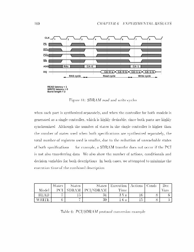
160 CHAPTER 6. EXPERIMENTAL RESULTS
CLK 1 2 3 4 5 6 7 8
CS
RAS
CAS
WE
RAsADD CA−0 CA−1
CA−0−a CA−0−b CA−1−a CA−1−b
RAS cycle Read cycle Write cycle
DQ
READ latency = 1WRITE latency = 0Burst length = 2
Figure 44: SDRAM read and write cycles
when each part is synthesized separately, and when the controller for both models is
generated as a single controller, which is highly desirable, since both parts are highly
synchronized. Although the number of states in the single controller is higher than
the number of states used when both speci�cations are synthesized separately, the
total number of registers used is smaller, due to the reduction of unreachable states
of both speci�cations | for example, a SDRAM transfer does not occur if the PCI
is not also transferring data. We also show the number of actions, conditionals and
decision variables for both descriptions. In both cases, we attempted to minimize the
execution time of the combined description.
States States States Execution Actions Conds. Dec.
Model PCI SDRAM PCI/SDRAM Time Vars.
READ 7 15 34 3.5 s 16 8 6
WRITE 6 7 30 1.6 s 15 8 3
Table 6: PCI/SDRAM protocol conversion example

6.3. CONTROL-UNIT FOR XMIT FRAME 161
6.3 Control-Unit for Xmit frame
CCT’
CCT’
CCT’
CCT’
CCT’
CCT’
discon_b = 0;xmitidle = 1;wait (txstart);xmitidle = 0;wait(DMAxmit);
st = ‘PREAMBLE;counter = 1;parity = 8’hff;
ether_xmit = preamble;txrestart = 0;discon_b = 1;if (counter < npreamble) counter = counter + 1;else state = SFD;
ether_xmit = sfd;b = DMAxmit;state = DEST1;
ether_xmit = b;parity = parity ^ b;b = DMAxmit;state = DEST2;
ether_xmit = b;parity = parity ^ b;b = DMAxmit;if (counter < length) counter = counter + 1;else state = DATAEND;
Figure 45: Program state machine for process xmit frame
We consider here the Ethernet coprocessor of Figure 2. In that �gure, let us focus
on the transmission unit. As mentioned in Example 5.4.18, the transmission unit is
composed of three processes, dma xmit, xmit frame and xmit bit. Upon receiving a
byte from process xmit frame, xmit bit sends the corresponding bit streams over the
line TXD. Thus, xmit bit must receive each byte eight cycles apart, which constrains
the rate at which the bytes are transmitted from xmit frame.
Process xmit frame was speci�ed as a program state machine written in Verilog

162 CHAPTER 6. EXPERIMENTAL RESULTS
HDL, as shown in Figure 45 [HLS], and it was also speci�ed with an exception han-
dling mechanism, i.e., the disable command of Verilog HDL. In the former implemen-
tation, because we have to abort the transmission of a frame if CCT becomes true, we
implemented the program state machine with a while loop which pools signal CCT, and
a case statement on variable state, which determines the next state of the program
state machine to be executed. Note that this state variable is not part of data ow
and it should be incorporated into the control-unit for xmit frame.
Since the execution of the while loop should be aborted if CCT becomes true, we re-
implemented the speci�cation for the program state machine of process xmit frame. In
this new speci�cation, we execute a sequential code that traverse the di�erent program
states of Figure 45, and we execute a watchdog in parallel with the new sequential
code. If condition CCT becomes true, then the watchdog will disable the execution
of the concurrent block containing both the sequential code and the watchdog. A
graphical representation of the speci�cation can be seen in Figure 46.
Table 7 presents the results for the scheduling of xmit frame from its control-
ow expression model. The �rst column shows the number of states of xmit-frame
before scheduling the operations. The second column shows the number of states
after state minimization. The third column shows the size of the constraints in terms
of BDD nodes, used by the BDD ILP solver. The fourth column shows the size of the
transition relation in terms of BDD nodes. The �fth column shows the execution time
taken to obtain a satisfying schedule minimizing the execution time of the process.
Note that by having a �nite-state representation of the behavior of the system in two
di�erent speci�cations, we were able to obtain two comparable implementations with
the same number of states.
In the table of Figure 7, note the di�erence between the sizes of the transition
relation of both implementations. Although the complexity of the CFE in the program
state machine case is larger than the complexity of the speci�cation using the disable
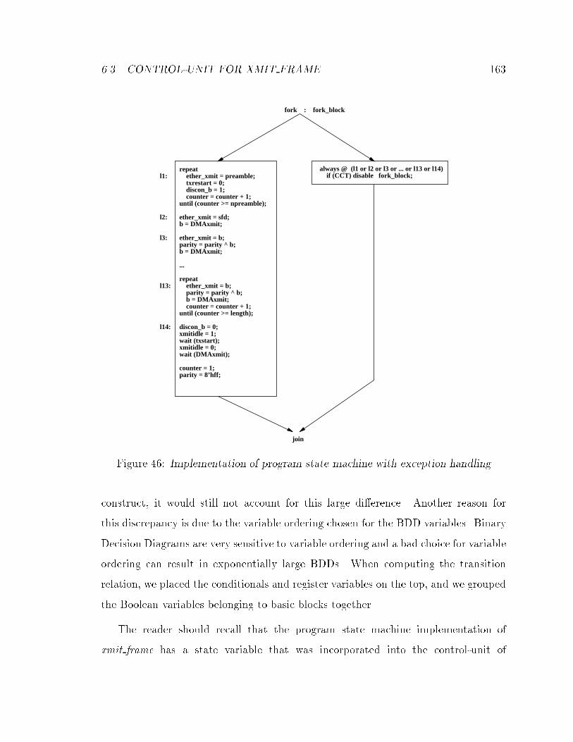
6.3. CONTROL-UNIT FOR XMIT FRAME 163
always @ (l1 or l2 or l3 or ... or l13 or l14) if (CCT) disable fork_block;
fork : fork_block
join
repeat ether_xmit = preamble; txrestart = 0; discon_b = 1; counter = counter + 1;until (counter >= npreamble);
ether_xmit = sfd;b = DMAxmit;
ether_xmit = b;parity = parity ^ b;b = DMAxmit;
...
repeat ether_xmit = b; parity = parity ^ b; b = DMAxmit; counter = counter + 1;until (counter >= length);
discon_b = 0;xmitidle = 1;wait (txstart);xmitidle = 0;wait (DMAxmit);
counter = 1;parity = 8’hff;
l1:
l2:
l3:
l13:
l14:
Figure 46: Implementation of program state machine with exception handling
construct, it would still not account for this large di�erence. Another reason for
this discrepancy is due to the variable ordering chosen for the BDD variables. Binary
Decision Diagrams are very sensitive to variable ordering and a bad choice for variable
ordering can result in exponentially large BDDs. When computing the transition
relation, we placed the conditionals and register variables on the top, and we grouped
the Boolean variables belonging to basic blocks together.
The reader should recall that the program state machine implementation of
xmit frame has a state variable that was incorporated into the control-unit of

164 CHAPTER 6. EXPERIMENTAL RESULTS
# States Constraint Trans. Rel. Time
xmit-frame (except.) 178 90 327 3022 4.3s
xmit-frame 178 90 995 24439 32.21s
Table 7: Results for the synthesis of xmit frame
xmit frame. This variable interacts with all basic blocks representing the states of
the program state machine, as it can be seen in Figure 45. As a result, no good vari-
able ordering can be found for this variable with respect to the ordering of variables
created for each basic block.
In order to smooth out the e�ects of a bad variable ordering for the state variable,
we ran both speci�cations on our program with the BDD using dynamic variable
ordering [Rud93]. The results are reported in Table 8.
# States Constraint Trans. Rel. Time
xmit-frame (except.) 178 90 327 3022 4.35s
xmit-frame 178 90 899 14149 402.64s
Table 8: Results for the synthesis of xmit frame with dynamic variable ordering of
BDDs
6.4 FIFO Controller
In this section, we will compare the results of our approach with the speci�cation of a
FIFO controller that was presented in [YW]. For this example, which is a sequential
model, we will show that we will not be able to obtain as good results as the ones
reported by [YW]. We will explain the design choices that we made that led to these
results. The reader must remember, however, that the approach presented in [YW]
cannot be used to synthesize the controllers for the examples presented previously.

6.4. FIFO CONTROLLER 165
incrementer
write register
read register
MAR
comparator
mux
RAM
wload rload
eq select mload r/w
data outdata in
read
write
Controller
Figure 47: Datapath for FIFO controller
Figure 47 presents the datapath for a FIFO controller. In this datapath, wload,
rload, select, mload and R/W are signals that must be generated to sensitize the
paths of the datapath. Signals eq, read and write are input signals to the controller.
A high-level view of the system is presented in Figure 48. In this �nite state
machine, also called in [YW] a BFSM, the states corresponds to basic blocks of the
speci�cation. For example, the IDLE basic block is represented by the CFE fmux(1) 0!
rload(1);mux(1)0! mar(1);mar(0)
0! r/w(1);mar(1)
1! mar(0); rload(1)
1! rload(0)g,
where signal(i) represents the condition of setting signal to value i. In addition to
the timing constraints implicit in the basic blocks, there are a number of path based
constraints in the speci�cation that must be satis�ed as well. For example, one of the
path based constraints that must be satis�ed is that at least two cycles must occur
between two writes of value 0 to signal r/w, i.e. min(2; r/w(0) r/w(0)). We are able
to obtain a controller for this speci�cation with 20 states before optimization in 1.778
s, with a constraint size of 86 BDD nodes and a transition relation of 2113 BDD
nodes.

166 CHAPTER 6. EXPERIMENTAL RESULTS
IDLE
WRITE READ
FULL EMPTY
eq eq
eq eq
read write
read write
Figure 48: High-level view of FIFO controller
In the solution found in [YW], the IDLE-READ-IDLE loop is reported to have 3
cycles. Using our approach, we obtained the same loop with 5 cycles. The reason for
this di�erence can be seen if we analyze how we handle constraints. We assumed the
0-1 ILP model for basic blocks, in which each basic block will take at least one cycle
to execute when all operations of the basic block can be executed in parallel. Now,
let us consider what happens when a path exists in the speci�cation that traverses n
basic blocks. In our model, we know that these n basic blocks will execute at least in
n cycles.
This restriction does not exist in the BFSM algorithm proposed in [YW]. In
this algorithm, the constraint on the minimum execution time is transferred from
the basic blocks to the loops. From Chapter 2 and Chapter 4, we know that all
loops must execute in at least one cycle. By removing the 1 cycle delay constraint of
basic blocks, the algorithm of [YW] is able to better compress the execution time of
sequential paths, and as a result, it is able to generate faster implementations such
as the one shown in this section. We will address this issue and some additional

6.4. FIFO CONTROLLER 167
improvements for our technique in the next chapter.
We must emphasize, however, that our approach is more complete in the sense
it can consider constraints traversing concurrent models, which cannot be considered
by [YW]. We can also consider register variables to be part of the speci�cation, which
cannot be easily incorporated by the BFSM representation.

Chapter 7
Conclusions and Future Work
7.1 Summary
We considered in this thesis modeling, analysis and synthesis techniques for concur-
rent and communicating, control- ow dominated designs, called system-level designs.
For these speci�cations, current synthesis tools cannot handle concurrency, synchro-
nization and exception handling and so they often achieve suboptimal results.
In order to best capture the degrees of freedom available in system-level designs,
we developed a modeling technique for control- ow dominated speci�cations, and we
presented a methodology for automatically obtaining the controllers for the concurrent
parts of the speci�cation. In particular, we focused in the following aspects of system-
level designs.
Modeling. We presented an algebraic model called control- ow expressions
to represent the control- ow of a system-level design. This model allowed us
to capture most of the control- ow constructs of speci�cation languages for
hardware, such as Verilog HDL, VHDL, StateCharts, Esterel and the C pro-
gramming language. Because it is common practice in structured programming
168

7.1. SUMMARY 169
to use variables to represent parts of the control- ow behavior of a speci�cation,
we allowed some variables of the speci�cation to be incorporated into control-
ow expressions. This added greater exibility to our model. We also allowed
control- ow structures to break the normal ow of execution, which was cap-
tured by an operation similar to the disable statement of Verilog.
Constraints. We showed how to specify complex design constraints of a sys-
tem. These constraints were not limited to timing and resource constraints,
but considered also the synchronization of concurrent parts of the design. In
addition, we were able to specify and consider constraints crossing concurrent
blocks of the design, which are generally ignored in other synthesis tools.
Analysis and Synthesis. We showed that control- ow expressions can be
analyzed by building the corresponding �nite-state machine, called a control-
ow �nite-state machine (CFFSM), which encodes the possible design choices,
and incorporates design constraints. We presented two synthesis techniques
for scheduling operations that satisfy the system's constraints. In the �rst
technique, called static scheduling, operations are scheduled statically on basic
blocks, but constraints can span over several basic blocks and control- ow con-
structs. In the second technique, called dynamic scheduling, we dynamically
schedule operations or parts of the design with respect to synchronization con-
straints, thus synchronizing the di�erent parts of the speci�cation with respect
to each other.
The solution of both scheduling problems are cast as Integer Linear Program-
ming instances and solved using Binary Decision Diagrams. There are two major
advantages in using BDDs to solve ILP problems. BDDs are able to represent
the whole space of solutions, instead of committing to a single solution that

170 CHAPTER 7. CONCLUSIONS AND FUTURE WORK
is obtained when using conventional ILP solvers. These solution space can be
used later to better constraint other parts of the design. Moreover, we showed
that BDDs allow us to consider a more compact constraint representation by
encoding the design choices using Gray or binary encoding.
Results. We showed how the techniques presented in this thesis can be used to
solve hard problems, such as the protocol conversion problem, the scheduling
problem for program state machines, and the scheduling problem for speci�ca-
tions with exception handling mechanisms. We also contrasted our modeling
and synthesis choices by showing the di�erences in the schedules obtained for
BFSMs.
7.2 Future Work
During the development of this work, we observed that several choices were made
that impacted the expressibility and synthesis results.
� Although using a model that includes concurrency, exception handling and vari-
ables increased the speci�cation and synthesis capabilities, the assumption that
every basic block executed in at least one cycle made by our approach compro-
mised the quality of the synthesis for sequential models. It is worth researching
a more general model where the one cycle constraint is imposed on loops only.
� We synchronized the concurrent parts of the design by dynamically scheduling
operations over time. As the reader may have noted, the complexity of the
dynamic scheduling technique may be too expensive at times. We believe that
it is worth researching new techniques for synchronization synthesis by investi-
gating automatic abstraction techniques for the speci�cations, or by developing
new techniques to achieve synchronization synthesis.

7.2. FUTURE WORK 171
� Since we used a model for analyzing the control- ow of the system by considering
all possible schedules, and we presented a technique for incorporating design
constraints from concurrent models, a natural extension to this is the veri�cation
of a system-level implementation. This could be achieved by considering our
model to be the speci�cation and the system's implementation to constraint
the design. Thus, checking for a feasible implementation in this problem is
equivalent to checking if the implementation satis�es the speci�cation and the
design constraints.
� The model we presented in our thesis can be extended to handle asynchronous
events, which is necessary in order to consider systems consisting of hardware
and software portions, that execute at di�erent rates. In particular, software
systems generally use a concurrency model better captured by interleaved con-
currency. Thus, a model for hardware/software codesign should consider inter-
leaved concurrency intermixed with the concurrency model presented for CFEs.

Bibliography
[Ake78] S.-B. Akers. Binary decision diagrams. IEEE Transactions on Comput-
ers, c-27, pp. 509{516, 1978.
[Bae90] J. C. M. Baeten. Process Algebra. Cambridge University Press, 1990.
[Bor88] G. Borriello. A new interface speci�cation methodology and its applica-
tion to transducer synthesis. UCB/CSD Technical Report (Dissertation)
88/430, U. C. Berkeley, 1988.
[BRB90] K. S. Brace, R. L. Rudell, and R. E. Bryant. E�cient implementation
of a bdd package. In Proceedings of the Design Automation Conference,
pp. 40{45, Orlando, FL, June 1990.
[Bry86] R. E. Bryant. Graph-based algorithms for boolean function manipula-
tion. IEEE Transactions on Computers, pp. 677{691, August 1986.
[Bry92] R. E. Bryant. Symbolic boolean manipulation with ordered binary-
decision diagrams. ACM Computing Surveys, pp. 293{318, September
1992.
[Brz64] J. A. Brzozowski. Derivatives of regular expressions. Journal of the
Association for Computing Machinery, 11(4), pp. 481{494, October 1964.
172

BIBLIOGRAPHY 173
[BS91] F. Boussinot and R. De Simone. The ESTEREL language. Proceedings
of the IEEE, 79(9), pp. 1293{1303, September 1991.
[Cam76] R. H. Campbell. Path Expressions: A Technique for Specifying Process
Synchronization. PhD thesis, University of Illinois, Urbana-Champaign.
Department of Computer Science, August 1976. UIUCDCS-R-77-863.
[Cam91] R. Camposano. Path-based scheduling for synthesis. IEEE Transactions
on CAD/ICAS, 10(1), pp. 85{923, January 1991.
[CBH+91] R. Camposano, R. A. Bergamaschi, C. E. Haynes, M. Payer, and S. M.
Wu. The ibm high-level synthesis system. In R. Camposano and Wayne
Wolf, editors, High-Level VLSI Synthesis, pp. 79{104. Kluwer Academic
Publishers, June 1991.
[CE81] E. M. Clarke and E. A. Emerson. Design and synthesis of synchronization
skeletons using branching time temporal logic. Technical Report TR-12-
81, Harvard University, 1981.
[CHJ+90] H. Cho, G. Hachtel, S. Jeong, E. Schwarz, and F. Somenzi. Atpg aspects
of fsm veri�cation. In Proceedings of the International Conference on
Computer-Aided Design, pp. 134{137, Santa Clara, November 1990.
[Cho74] Y. Choueka. Theories of automata on !-tapes: A simpli�ed approach.
Journal of Computer and System Sciences, 8, pp. 117{141, 1974.
[CLR90] T. H. Cormen, C. E. Leiserson, and R. L. Rivest. Introduction to Algo-
rithms. MIT Press, 1990.
[CM90] O. Coudert and J. C. Madre. A uni�ed framework for the formal veri�ca-
tion of sequential circuits. In Proceedings of the International Conference
on Computer-Aided Design, pp. 126{129, Santa Clara, November 1990.

174 BIBLIOGRAPHY
[DDT83] M. Davio, J.-P. Deschamps, and A. Thayse. Digital Systems with Algo-
rithm Implementation. John Wiley & Sons, 1983.
[DGL92] A. Wu D. Gajski, N. Dutt and S. Lin. High-Level VLSI Synthesis -
Introduction to Chip and System Design. Kluwer Academic Publishers,
1992.
[DH86] D. Drusinsky and D. Harel. Statecharts as an abstract model for digital
control-units. Technical Report CS86-12, Weizmann Institute of Science,
1986.
[DKMT90] G. DeMicheli, D. C. Ku, F. Mailhot, and T. Truong. The olympus
synthesis system for digital design. IEEE Design and Test Magazine,
pp. 37{53, October 1990.
[FKJM93] D. Filo, D. C. Ku, C. N. Coelho Jr., and G. De Micheli. Interface opti-
mization for concurrent systems under timing constraints. IEEE Trans-
actions on VLSI Systems, 1(3), pp. 268{281, September 1993.
[FYDM93] J. Fron, J. Yang, M. Damiani, and G. De Micheli. Synthesis framework
based on trace and automata theory. In International Workshop on Logic
Synthesis, Tahoe, CA, May 1993.
[Geb91] C. H. Gebotys. Optimal VLSI Architectural Synthesis. Kluwer Academic
Publishers, 1991.
[GG92] V. K. Garg and M. T. Gagunath. Concurrent regular expressions and
their relationship to petri-nets. Theoretical Computer Science, 96(2), pp.
285{304, 1992.
[GJM92] R. K. Gupta, C. N. Coelho Jr., and G. De Micheli. Synthesis and sim-
ulation of digital systems containing interacting hardware and software

BIBLIOGRAPHY 175
components. In Proceedings of the 29thDesign Automation Conference,
pp. 225{230, June 1992.
[GJM94] R. K. Gupta, C. N. Coelho Jr., and G. De Micheli. Program imple-
mentation schemes for hardware-software systems. IEEE Computer, pp.
48{55, January 1994.
[GPR93] L. Guerra, M. Potkonjak, and J. Rabaey. High level synthesis for re-
con�gurable datapath structures. In Proceedings of the International
Conference on Computer-Aided Design, pp. 26{29, November 1993.
[Gup93] R. K. Gupta. Co-synthesis of Hardware and Software for Digital Embed-
ded Systems. PhD thesis, Stanford University, 1993.
[GVNG94] D. Gajski, F. Vahid, S. Narayan, and J. Gong. Speci�cation and Design
of Embedded Systems. Prentice Hall, 1994.
[HB84] K. Hwang and F. A. Briggs. Computer Architecture and Parallel Pro-
cessing. McGraw-Hill Book Company, 1984.
[HLH91] C.-T. Hwang, J.-H. Lee, and Y-C Hsu. A formal approach to the schedul-
ing problem in high-level synthesis. IEEE Transactions on CAD/ICAS,
10(4), pp. 464{475, April 1991.
[HLS] Benchmarks of the 1992 high-level synthesis workshop.
[HP82] L. Hafer and A. Parker. Automated synthesis of digital hardware. IEEE
Transactions on CAD/ICAS, c-31(2), February 1982.
[HP92] Y.-H. Hung and A. C. Parker. High-level synthesis with pin constraints
for multiple-chip designs. In Proceedings of the Design Automation Con-
ference, pp. 231{234, June 1992.
176 BIBLIOGRAPHY
[HU79] J. E. Hopcroft and J. D. Ullman. Introduction to Automata Theory,
Languages and Computation. Addison Wesley, 1979.
[Hu95] A. J. Hu. Techniques for E�cient Formal Veri�cation Using Binary
Decision Diagrams. PhD thesis, Stanford University, 1995.
[JS93] S.-W. Jeong and F. Somenzi. Logic Synthesis and Optimization, chap-
ter A New Algorithm for 0-1 Programming Based on Binary Decision
Diagrams, pp. 145{166. Kluwer Academic Plublishers, 1993.
[KD90] D. C. Ku and G. DeMicheli. HardwareC - a language for hardware
design (version 2.0). CSL Technical Report CSL-TR-90-419, Stanford,
April 1990.
[Keu89] K. Keutzer. Three competing design methodologies for asics: Architec-
tural synthesis, logic synthesis, and module generation. In Proceedings
of the Design Automation Conference, pp. 308{313, June 1989.
[Kle56] S. C. Kleene. Representation of Events by Nerve Nets In C. E. Shan-
non and J. McCarthy, editors, Automata Studies, pp. 3{42. Princeton
University Press, 1956.
[KLL91] T. Kim, J. W. S. Liu, and C. L. Liu. A scheduling algorithm for condi-
tional resource sharing. In Proceedings of the International Conference
on Computer-Aided Design, pp. 84{87, Santa Clara, November 1991.
[KLMM95] D. Knapp, T. Ly, D. MacMillen, and R. Miller. Behavioral synthesis
methodology for hdl-based speci�cation and validation. In Proceedings
of the Design Automation Conference, pp. 286{291, June 1995.
[KM92] D. Ku and G. De Micheli. High-level Synthesis of ASICs under Tim-
ing and and Synchronization Constraints. Kluwer Academic Publishers,

BIBLIOGRAPHY 177
1992.
[KOH+94] J. Kuskin, D. Ofelt, M. Heinrich, J. Heinlein, R. Simoni, K. Ghara-
chorloo, J. Chapin, D. Nakahira, J. Baxter, M. Horowitz, A. Gupta,
M. Rosenblum, and J. Hennessy. The Stanford FLASH multiprocessor.
In Proceedings of the International Symposium on Computer Architec-
ture, pp. 302{313, June 1994.
[Lan91] D. Lanneer et. al. Architectural synthesis for medium and high through-
put signal processing with the new cathedral environment. In R. Cam-
posano and Wayne Wolf, editors, High-Level VLSI Synthesis, pp. 27{54.
Kluwer Academic Publishers, June 1991.
[Las90] J. Laski. Path expressions in data ow program testing. In 14th Anual
International Computer Software and Applications Conference, pp. 570{
576, Chicago, 1990.
[LSU89] R. Lipsett, C. Schaefer, and C. Ussery. VHDL: Hardware Description
and Design. Kluwer Academic Publishers, 1989.
[Mar90] P. Marwedel. Matching system and component behaviour in mimola
synthesis tool. In Proceedings of the European Design Automation Con-
ference, pp. 146{156, March 1990.
[McM93] K. McMillan. Symbolic Model Checking. Kluwer Academic Publishers,
1993.
[Mea55] G. H. Mealy. A method for synthesizing sequential circuits. Bell System
Technical Journal, 34(5), pp. 1045{1079, 1955.
[Mic94] G. De Micheli. Synthesis and Optimization of Digital Circuits. McGraw
Hill, 1994.

178 BIBLIOGRAPHY
[Mil84] R. Milner. A complete inference system for a class of regular behaviours.
Journal of Computer and System Sciences, 28, pp. 439{467, 1984.
[Mil85] G. J. Milne. Circal and the representation of communication, concur-
rency, and time. ACM Transactions on Programming Languages and
Systems, 7(2), pp. 270{298, April 1985.
[Mil91] R. Milner. Handbook of Theoretical Computer Science, volume 2, chapter
19: Operational and Albebraic Semantics of Concurrent Processes, pp.
1201{1242. MIT Press, 1991.
[Mil94] G. Milne. Formal Speci�cation and Veri�cation of Digital Systems.
McGraw-Hill, 1994.
[Moo56] E. F. Moore. Gedanken-Experiments on Sequential Machines, In
C. E. Shannon and J. McCarthy, editors, Automata Studies, pp. 129{
153. Princeton University Press, 1956.
[MPC90] M. McFarland, A. Parker, and R. Camposano. The high-level synthesis
of digital systems. Proceedings of the IEEE, 78(2), pp. 301{318, February
1990.
[NEC93] NEC Memory Products Data Book, 1993.
[Nem88] G. Nemhauser. Integer and Combinatorial Optimization. John Wiley &
Sons, 1988.
[NFCM92] S. Note, G. Goossens F. Catthoor, and H. De Man. Combined hardware
selection and pipelining in high-performance data-path design. IEEE
Transactions on CAD/ICAS, 11(4), pp. 413{423, April 1992.

BIBLIOGRAPHY 179
[NG95] S. Narayan and D. Gajski. Interfacing incompatible protocols using in-
terface process generation. In Proceedings of the Design Automation
Conference, pp. 468{473, June 1995.
[NT86] J. Nestor and D. Thomas. Behavioral synthesis with interfaces. In Pro-
ceedings of the Design Automation Conference, pp. 112{115, June 1986.
[Pai77] M. R. Paige. On partitioning program graphs. IEEE Transactions on
Software Engineering, SE-3(6), pp. 386{393, November 1977.
[PCI95] PCI Local Bus Speci�cation Revision 2.1, 1995.
[Pet81] J. L. Peterson. Petri Net Theory and the Modeling of Systems. Prentice-
Hall, 1981.
[RB93] I. Radivojevi�c and F. Brewer. Symbolic techniques for optimal schedul-
ing. In Proceedings of the Synthesis and Simulation Meeting and In-
ternational Interchange { SASIMI, pp. 145{154, Nara, Japan, October
1993.
[RHSJ94] J.-K. Rho, G. D. Hachtel, F. Somenzi, and R. M. Jacoby. Exact and
heuristic algorithms for the minimization of incompletely speci�ed state
machines. IEEE Transactions on CAD/ICAS, 13(2), pp. 167{177, Febru-
ary 1994.
[Rud74] S. Rudeanu. Boolean Functions and Equations. North-Holland, 1974.
[Rud93] R. Rudell. Dynamic variable ordering for ordered binary decision dia-
grams. In International Workshop on Logic Synthesis, Lake Tahoe, CA,
April 1993.
[Sar89] R. Saracco. Telecommunications Systems Engineering Using SDL. Else-
vier Science, 1989.

180 BIBLIOGRAPHY
[Sea94] A. Seawright. Grammar-Based Speci�cation and Synthesis for Syn-
chronous Digital Hardware Design. PhD thesis, UC Santa Barbara, 1994.
[Sta70] E. Stabler. Microprogram transformations. IEEE Transactions on Com-
puters, c-19, pp. 908{916, 1970.
[TM91] D. E. Thomas and P. R. Moorby. The Verilog hardware description
language. Kluwer Academic Publishers, 1991.
[TSL+90] H. J. Touati, H. Savoj, B. Lin, R. K. Brayton, and A. Sangiovanni-
Vincentelli. Implicit state enumeration of �nite state machines using
bdd's. In Proceedings of the International Conference on Computer-
Aided Design, pp. 130{133, Santa Clara, November 1990.
[TU82] H. W. Trickey and J. D. Ullman. A regular expression compiler. In IEEE
COMPCON, pp. 345{348, 1982.
[TWL95] A. Takach, W. Wolf, and M. Leeser. An automaton model for scheduling
constraints. IEEE Transactions on Computers, 44(1), pp. 1{12, January
1995.
[VRB+93] J. Vanhoof, K. V. Rompaey, I. Bolsens, G. Goossens, and H. De Man.
High-level Synthesis for Real-time Digital Signal Processing. Kluwer Aca-
demic Publishers, 1993.
[Wan88] T. H. Wang. Repeatable Firing Sequences for Petri Nets under Con-
ventional, Subset and Timed Firing Rules. PhD thesis, Case Western
Reserve University, 1988.
[Wol82] P. L. Wolper. Synthesis of Communicating Processes from Temporal
Logic Speci�cations. PhD thesis, Stanford University, 1982.
BIBLIOGRAPHY 181
[WT92] K. Wakabayashi and H. Tanaka. Global scheduling independent of con-
trol dependencies based on condition vectors. In Proceedings of the De-
sign Automation Conference, pages pp. 112{115, June 1992.
[WTHM92] W. Wolf, A. Takach, C. Huang, and R. Manno. The Princeton university
behavioral synthesis system. In Proceedings of the 29thDesign Automa-
tion Conference, pp. 182{187, June 1992.
[WTL91] W. Wolf, A. Takach, and T. Lee. High-Level VLSI Synthesis, R. Cam-
posano and W. Wolf, editors, in Architectural Optimization Methods for
Control-Dominated Machines. Kluwer Academic Publishers, 1991.
[YW] T.-Y. Yen and W. Wolf. Optimal scheduling for minimumdependence in
fsms. Accepted for publication in IEEE Transactions on VLSI Systems.
[Zhu92] Z. Zhu. Structured Hardware Design Transformations. PhD thesis, Indi-
ana University, 1992.
[ZJ93a] Z. Zhu and S. D. Johnson. Automatic synthesis of sequential synchro-
nization. In IFIP Conference on Hardware Description Languages and
their Applications (CHDL '93), Ottawa, Canada, April 1993.
[ZJ93b] Z. Zhu and S. D. Johnson. An example of interactive hardware transfor-
mation. Technical Report 383, Indiana University, 1993.
[ZJ94] Z. Zhu and S. D. Johnson. Capturing synchronization speci�cations for
sequential compositions. In Proceedings of the International Conference
on Computer Design, pp. 117{121, October 1994. also as University of
British Columbia TR 93-3.
Appendix A
Algebra of Synchronous Processes
In this section we de�ne the algebra of synchronous processes (ASP), in a manner
similar to the de�nitions found in [Bae90].
De�nition A.1 Let A = (�ASP; �; �; ; EASP) be the model de�ned as follows.
� The alphabet of symbols of �ASP denote the set of actions and the set of oper-
ations.
{ Actions are 0-ary functions and correspond to the atomic symbols.
{ Operations +,� and j are binary functions and correspond to alternative,
sequential and synchronous parallelism compositions, respectively.
� The two symbols � and � are de�ned as a deadlock and empty process, respec-
tively.
� The function is a partial function de�ned as : �ASP[f�g��ASP[f�g !
�ASP[f�; �g. One special symbol of �ASP is denoted by 1 which is considered
a unit element of , i.e., (a; 1) = (1; a) = a, for all actions a of �ASP. The
empty process � is considered a zero element of , i.e., (a; �) = (�; a) = �, for
all actions a of �ASP.
182
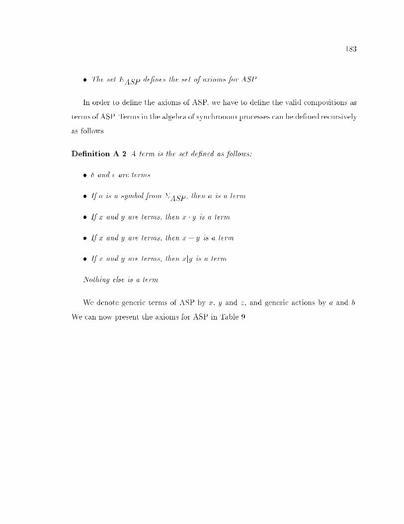
183
� The set EASP de�nes the set of axioms for ASP.
In order to de�ne the axioms of ASP, we have to de�ne the valid compositions as
terms of ASP. Terms in the algebra of synchronous processes can be de�ned recursively
as follows.
De�nition A.2 A term is the set de�ned as follows:
� � and � are terms.
� If a is a symbol from �ASP, then a is a term.
� If x and y are terms, then x � y is a term.
� If x and y are terms, then x+ y is a term.
� If x and y are terms, then xjy is a term.
Nothing else is a term.
We denote generic terms of ASP by x, y and z, and generic actions by a and b.
We can now present the axioms for ASP in Table 9.

184 APPENDIX A. ALGEBRA OF SYNCHRONOUS PROCESSES
x+ y = y + x A1(x+ y) + z = x+ (y + z) A2
x+ x = x A3(x+ y) � z = x � z + y � z A4(x � y) � z = x � (y � z) A5x+ � = x A6� � x = � A7
x � � = x A8� � x = x A9ajb = (a; b) CF1 and CF2a � xjb = (ajb) � x SC1ajb � y = (ajb) � y SC2
a � xjb � y = (ajb) � (xjy) SC3(x+ y)jz = (xjz) + (yjz) SC4xj(y + z) = (xjy) + (xjz) SC5xj� = � SC6�jx = � SC7
Table 9: Axioms for ASP

Appendix B
Binary Decision Diagrams
Binary Decision Diagrams [Bry86, Bry92] are a compact graph representation for
Boolean functions based on the decision diagrams of Akers [Ake78]. A BDD rep-
resents a Boolean function by inferring all true and false values of the function by
path traversals on the graph. A formal de�nition of BDDs due to Bryant [Bry86] is
presented below.
De�nition B.1 A Binary Decision Diagram is a rooted, directed graph with vertex
set V containing two types of vertices. A nonterminal vertex v has as attributes
an argument index index(v) 2 f1; . . . ; ng and two children low(v); high(v) 2 V . A
terminal vertex v has as attribute a value value(v) 2 f0; 1g.
The correspondence between a BDD and a Boolean function can be seen from the
following de�nition:
De�nition B.2 A BDD G having root vertex v denotes a function fv, de�ned recur-
sively as:
1. If v is a terminal vertex:
(a) If value(v) = 1, then fv = 1.
185

186 APPENDIX B. BINARY DECISION DIAGRAMS
(b) If value(v) = 0, then fv = 0.
2. If v is a nonterminal vertex with index(v) = i, then fv is the function:
fv = xi flow(v) _ xi fhigh(v)
In addition to that, a BDD is reduced if low(v) 6= high(v) for every vertex v 2 V ,
and it is ordered if index(v) < index(low(v)) and index(v) < index(high(v)) for
every nonterminal v.
Reduced ordered BDDs (ROBDDs) play an important role in Boolean function
manipulation because they are canonical, i.e. if two BDDs are isomorphic, then they
represent the same Boolean function. In this thesis, we will be referring to ROBDDs
by BDDs.
x1
x2
1 0
then
else
then else
Figure 49: Binary Decision Diagram for function x1x2
Example B.1.1. The function f(x1; x2) = x1x2 can be represented by the
BDD of Figure 49.
In this BDD, any path leading to vertex 1 represent an assignment to the
variables that yields a true value for the Boolean function f , and a path leading
to vertex 0 represent an assignment to the variables that yields a false value
for the f . 2
BDDs have been used in several di�erent applications, including the solution of In-
teger Linear Programming [JS93] described earlier, because of its low space complexity

187
to represent some types of Boolean functions. In these problems, each equation of the
ILP problem is converted into a Boolean function [Rud74], which is represented by a
BDD. This Boolean function contains all valid assignments to the Boolean variables
that satisfy the ILP equation. Since in an ILP instance of the problem is speci�ed
as a set of equations and a cost function that should be minimized, an assignment
satisfying this set of constraints can be obtained by conjoining the BDDs for the dif-
ferent equations, and a solution that minimizes a cost function can be obtained by a
branch-and-bound on the set of valid assignments to the resulting BDD with respect
to the cost function [JS93].
0 1
x
x
2
1
then else
then else
Figure 50: BDD representing the constraint 4x1 + 5x2 � 8
Example B.1.2. The equation 4x1 + 5x2 � 8 is true by any assignment
satisfying the Boolean formula x1 _ x2, whose BDD is shown in Figure 50. 2