Learning Nonparametric Forest Graphical Models with Prior

Information

Yuancheng Zhu, Zhe Liu

University of Chicago

Siqi Sun

Toyota Technological Institute at Chicago

Abstract

We present a framework for incorporating prior information into nonparametric estimationof graphical models. To avoid distributional assumptions, we restrict the graph to be a forestand build on the work of forest density estimation (FDE). We reformulate the FDE approachfrom a Bayesian perspective, and introduce prior distributions on the graphs. As two concreteexamples, we apply this framework to estimating scale-free graphs and learning multiple graphswith similar structures. The resulting algorithms are equivalent to finding a maximum spanningtree of a weighted graph with a penalty term on the connectivity pattern of the graph. We solvethe optimization problem via a minorize-maximization procedure with Kruskal’s algorithm.Simulations show that the proposed methods outperform competing parametric methods, andare robust to the true data distribution. They also lead to improvement in predictive powerand interpretability in two real data sets.

1 Introduction

Graphical models are widely used to encode the conditional independence relationships betweenrandom variables. In particular, a random vector X = (X1, . . . , Xd) is represented by an undirectedgraph G = (V,E) with d = |V | vertices and missing edges (i, j) 6∈ E whenever Xi and Xj areconditionally independent given the other variables. One major statistical task is to learn thegraph from n i.i.d. copies of the random vector.

Existing approaches for estimating graphical models make assumptions on either the underly-ing distribution or the graphical structure. Currently the most popular method, called graphicallasso [6], assumes that the random vector follows a multivariate Gaussian distribution. In thisway, learning the graph is equivalent to estimating the precision matrix Ω, since the conditionalindependence of a Gaussian random vector is entirely determined by the sparsity pattern of Ω. Thegraphical lasso finds a sparse estimate of Ω by maximizing the `1-regularized log-likelihood. On theother hand, we can make no distributional assumptions but restrict the graph to be a forest instead.Under this structural constraint, there exists a factorization of the density function involving only

1

arX

iv:1

511.

0379

6v2

[st

at.M

E]

25

May

201

6

the univariate and bivariate marginal densities, which makes nonparametric estimation tractablein high dimensions. In this case, estimating the graph amounts to finding the maximum spanningtree of a weighted graph; see, for example, [2, 10] for details.

Oftentimes, additional information on the structure of a graph is available a priori, which couldbe utilized to assist the estimation task. For example, a wide variety of the networks in recentliterature, such as protein, gene, and social networks, are reported to be scale-free. That is, thedegree distribution of the vertices follows a power law: p(degree = k) ∝ k−α for some α > 1. Insuch scale-free networks, some vertices have many more connections than others, and these highest-degree vertices are usually called hubs and serve significant roles in their networks. As anotherexample of prior information, consider the applications where we believe that several networksshare similar but not necessarily identical structures. This phenomenon is not unusual when wehave multiple sets of data across distinct classes or units, such as gene expression measurementscollected on a set of normal tissue samples and a set of cancer tissue samples. It is thus natural toask whether such prior information can be integrated to improve the estimation.

Various approaches have been proposed to incorporate the prior belief of the underlying graphs,for example, [4, 11, 13, 14] for learning scale-free graphical models, and [7, 3, 12, 15] for jointestimation of multiple graphical models. Nevertheless, to the best of our knowledge, all the existingmethods assume some parametric distribution on the data, mostly multivariate Gaussian. Suchdistributional assumptions can be quite unrealistic and unnecessary in many applications. Eventhough the marginal distribution of each variable can be transformed to approximately Gaussian,which allows arbitrary univariate distributions, the joint dependence is still restricted under theGaussian assumption.

In this paper, we relax such distributional assumptions and estimate graphical models non-parametrically. We build on the forest density estimation (FDE) method introduced in [10]. Inparticular, we reformulate the FDE approach from a Bayesian perspective, and encode the priorinformation by putting some prior distribution on the graphs, which favors those that are moreconsistent with our prior belief. We further show that for the scale-free-graph case and the multiple-graph case, such an approach amounts to finding a maximum spanning tree of a weighted graphwith a penalty term on the connection pattern of the nodes. We then devise an algorithm basedon a minorize-maximization procedure and Kruskal’s algorithm [9] to find a local optimal solution.

The rest of the paper is organized as follows. In the following section, we give background onforest density estimation. In Section 3, we first give a general framework on how to incorporateprior information to nonparametric forest-based graphical model estimation, and then illustratehow the framework can be specialized to model scale-free graphical models and jointly estimatemultiple graphical models with similar structure. In Section 4, we provide a brief review on therelated work. Experimental results on synthetic data sets and real applications are presented inSection 5, followed by a conclusion in Section 6.

2 Forest density estimation

We say an undirected graph is a forest if it is acyclic. Let F = (VF , EF ) be a forest with verticesVF = 1, . . . , d and edge set EF ∈ VF × VF . Let X = (X1, . . . , Xd) be a d-dimensional randomvector with density p(x) > 0. We say that X, or equivalently, its density p, is Markov to F ifXi and Xj are conditionally independent given the other random variables whenever edge (i, j) is

2

missing in EF . A density p that is Markov to F has the following factorization

p(x) =∏

(i,j)∈EF

pij(xi, xj)

pi(xi)pj(xj)

∏`∈VF

p`(x`), (1)

where each pij(xi, xj) is a bivariate density and each pl(xl) is a univariate density. With thisfactorization, we can write the expected log-likelihood as

E log p(X) =

∫p(x)

∑(i,j)∈EF

logpij(xi, xj)

pixipj(xj)+∑`∈VF

log p`(x`)

dx (2)

=∑

(i,j)∈EF

I(Xi;Xj)−∑`∈VF

H(X`), (3)

where I(Xi;Xj) =∫pij(xi, xj) log

pij(xi,xj)pi(xi)pj(xj)

dxidxj is the mutual information between Xi and Xj ,

and H(X`) = −∫p`(x`) log p`(x`)dx` is the entropy of X`. We maximize the right hand side of (3)

to find the optimal forest F

F = arg maxF∈Fd

∑(i,j)∈EF

I(Xi;Xj), (4)

where Fd is the collection of spanning trees on vertices 1, . . . , d. We let Fd contain only spanningtrees because there is always a spanning tree that solves the problem (4). This problem can berecast as the problem of finding a maximum spanning tree for a weighted graph, where the weightwij of the edge between nodes i and j is I(Xi;Xj). Kruskal’s algorithm [9] is a greedy algorithmthat is guaranteed to find an optimal solution, while Chow and Liu [2] propose the procedure inthe setting of discrete random variables. The method is described in Algorithm 1.

Algorithm 1 Kruskal’s (Chow-Liu) algorithm

Input Weight matrix W = (wij)d×dInitialize E(0) ← ∅for ` = 1, . . . , d− 1 do

(i(`), j(`))← arg max(i,j) wij such that E(`−1) ∪ (i(`), j(`)) doesn’t contain a cycle

E(`) ← E(`−1) ∪ (i(`), j(`))end forOutput The final edge set E(d−1)

However, this procedure is not practical since the true density p is unknown. Suppose insteadthat we have X1,1:d, . . . , Xn,1:d, which are n i.i.d. copies of the random vector X. We replace thepopulation mutual information by the estimates

I(Xi;Xj) =

∫pij(xi, xj) log

pij(xi, xj)

pi(xi)pj(xj)dxidxj , (5)

where pij(xi, xj) and p`(x`) are kernel density estimators of the bivariate and univariate marginaldensities

pij(xi, xj) =1

n

n∑t=1

1

h22K

(Xti − xih2

)K

(Xtj − xj

h2

), p`(x`) =

1

n

n∑t=1

1

h1K

(Xt` − x`

h1

)(6)

3

with a kernel function K and bandwidths h2 and h1. The resulting estimator of the graph becomes

F = arg maxF∈Fd

∑(i,j)∈EF

I(Xi;Xj). (7)

A held-out set is usually used to prune the spanning tree F by stopping early in Algorithm 1 whenthe likelihood on the held-out set is maximized. Thus we obtain a forest estimate of the graph.

3 Learning forest graphical model with prior knowledge

3.1 A Bayesian framework

Sometimes we have some prior information about the structure of the underlying graphical models,and would like to incorporate that to assist the estimation. One way to realize that is to encodethe prior knowledge into prior distributions on the spanning trees. Let π(F ) be a prior distributionon Fd, the set of the spanning trees with d nodes. Given the data X1,1:d, . . . , Xn,1:d and assumingthe density p is known and Markov to the spanning tree F , we can write the likelihood as

p(X|F ) =

n∏t=1

∏(i,j)∈EF

pij(Xti, Xtj)

pi(Xti)pj(Xtj)

∏`∈VF

p`(Xt`)

. (8)

Then the posterior probability of F is

p(F |X) ∝ p(X|F )π(F ) ∝n∏t=1

∏(i,j)∈EF

pij(Xti, Xtj)

pi(Xti)pj(Xtj)

∏k∈VF

pk(Xtk)

· π(F ). (9)

The maximum a posteriori (MAP) estimate is given by

Fmap = arg maxF∈Fd

∑(i,j)∈EF

n∑t=1

1

nlog

pij(Xti, Xtj)

pi(Xti)pj(Xtj)+

1

nlog π(F )

. (10)

Since we do not know the true density p in practice, we can plug in the estimator (5) and obtain

Fπ = arg maxF∈Fd

∑(i,j)∈EF

I(Xi;Xj) +1

nlog π(F )

(11)

as an approximation of Fmap. In fact, Fπ is obtained by replacing the true marginal densities andthe empirical distributions in (10) by their corresponding density estimates. It can also be viewedas a penalized version of the estimator (7).

The penalty term 1n log π(F ), which is sometimes combinatorial, could make the optimization

problem extremely hard to solve. However, when log π(F ) is convex with respect to the entriesof the adjacency matrix of F , we can adopt a minorize-maximization algorithm [8] to find a localoptimal solution. In fact, given the convexity of log π(F ), the objective function adopts a linearlower bound at any current estimates. This linear lower bound can be then decomposed into a sumof weights over the edges, and we can apply the Kruskal’s algorithm to update our estimate. Weshall see in details in the following two concrete examples how this can be carried out.

4

3.2 Scale-free graphs

Now suppose that we have reasons to believe that the graph is scale-free, or more generally, thatthe graph consists of several nodes that have dominating degrees compared to the rest. Let δ(F, l)be the degree of the node l of a spanning tree F ∈ Fd. Consider a prior distribution on F whichsatisfies

π(F ) ∝∏`∈VF

δ(F, `)−α, (12)

for some α > 1. This prior distribution favors the spanning trees whose degrees have a power lawdistribution, and thus reflects our prior beliefs. Plugging this in (11), we obtain

Fπ = arg maxF∈Fd

∑(i,j)∈EF

I(Xi;Xj)− λ∑`∈VF

log(δ(F, `))

, (13)

where λ = α/n can be now viewed as a tuning parameter. To solve this optimization problem, wefirst rewrite the objective function as

f(F ) =∑i<j

wijFij − λd∑i=1

log

d∑j=1

Fij

, (14)

where wij = I(Xi;Xj). Here we also abuse our notation by writing F as the adjacency matrix ofF , that is, Fij = 1 if and only if (i, j) ∈ EF . Note that we have the additional constraint that thegraph F is a spanning tree. Given a current estimate F , we first lower bound f(F ) by linearizingit at F :

f(F ) ≥∑i<j

wijFij − λd∑i=1

log

d∑j=1

Fij

+

∑dj=1 Fij −

∑dj=1 Fij∑d

j=1 Fij

(15)

=∑i<j

(wij −

λ∑d`=1 Fi`

− λ∑d`=1 Fj`

)Fij + C, (16)

where C is a constant which doesn’t depend on F . We can maximize this lower bound by applyingKruskal’s algorithm to the graph with edge weights

wij = wij −λ∑d

`=1 Fi`− λ∑d

`=1 Fj`. (17)

We see that the weights are updated at each iteration based on the current estimate of the graph.Each edge weight is penalized by two quantities that are inversely proportional to the degrees of thetwo endpoints of the edge. An edge weight is thus penalized less if its endpoints are already highlyconnected and vice versa. With such a “rich gets richer” procedure, the algorithm encourages somevertices to have high connectivity and hence the overall degree distribution to have a heavy tail. Weiterate through such minorization and maximization steps until convergence. Since the objectivefunction is always increasing, the algorithm is guaranteed to converge to a local maximum.

5

3.3 Multiple graphs with similar structure

In this part, we illustrate how the framework can be modified to facilitate the case where wehave multiple graphs that are believed to have similar but not necessarily identical structures.Instead of one single graph, suppose that we now have K graphical models with underlying forestsF (1), . . . , F (K), and for the kth one, we observe data X(k) = (X1,1:d, . . . , Xnk,1:d). Given a jointprior distribution π on (F (1), . . . , F (K)), we combine the likelihood for the K models and updatethe posterior distribution (9) to be

p(F (1:K)|X(1:K)) ∝K∏k=1

n∏t=1

∏(i,j)∈E

F (k)

p(k)ij (X

(k)ti , X

(k)tj )

p(k)i (X

(k)ti )p

(k)j (X

(k)tj )

∏`∈V

F (k)

p(k)` (X

(k)t` )

· π(F (1:K)). (18)

Next, we design a prior distribution on the set of K spanning trees which reflects our belief that thestructures across the K of them share some similarity. Again we use F (k) to denote the adjacency

matrix of the corresponding graph, that is, F(k)ij = 1 if and only if (i, j) ∈ EF (k) . We consider the

following hierarchical model:

τij ∼ Beta(α, β) for all i < j, (19)

F(k)ij | τij ∼ Bernoulli(τij) for all k and i < j. (20)

According to this model, the same edge across multiple graphs is governed by the same parameterτij , and hence encourage similarity across them. This essentially gives a prior distribution on F (1:K):

π(F (1:K)) ∝∏i<j

∫τij

p(Fij | τij)p(τij)dτij · 1F (k) ∈ Fd for all k (21)

=∏i<j

∫τij

[K∏k=1

p(F(k)ij |τij)

]p(τij)dτij · 1F (k) ∈ Fd for all k (22)

∝∏i<j

∫τij

τα+‖Fij‖1−1ij (1− τij)β+K−‖Fij‖1−1dτij · 1F (k) ∈ Fd for all k (23)

=∏i<j

B(α+ ‖Fij‖1, β +K − ‖Fij‖1) · 1F (k) ∈ Fd for all k, (24)

where Fij is the vector containing the (i, j)th entries of F (k) for k = 1, . . . ,K, ‖ · ‖1 denotes the`1 norm, and B(·, ·) denotes the Beta function. Now combining this with (18) and following thereasoning in Subsection 3.1, we obtain our estimator in this case

F (1:K)π = arg max

F (k)∈Fd, ∀k

K∑k=1

∑(i,j)∈E

F (k)

I(X(k)i ;X

(k)j ) + λ

∑i<j

logB(α+ ‖Fij‖1, β +K − ‖Fij‖1)

.

(25)Note that we include an extra tuning parameter λ in front of the penalty term to give us a bit moreflexibility in controlling its magnitude. The function k 7→ logB(α + k, β + K − k) is convex andtakes larger values when k is close to 0 or K compared to those in between. Using it as a penaltythus favors the set of graphs which share common edges.

6

To solve (25), we again adopt a minorize-maximization procedure. Specifically, write the objec-tive function as

f(F (1:K)) =

K∑k=1

∑i<j

w(k)ij F

(k)ij + λ

∑i<j

logB(α+ ‖Fij‖1, β +K − ‖Fij‖1), (26)

where w(k)ij = I(X

(k)i ;X

(k)j ). Given a current solution F (k), we linearize f(F (1:K)) at F (k) and get

f(F (1:K)) ≥K∑k=1

∑i<j

w(k)ij F

(k)ij + λ

∑i<j

(‖Fij‖ − ‖Fij‖1)(ψ(α+ ‖Fij‖1)− ψ(β +K − ‖Fij‖1)

)(27)

=

K∑k=1

∑i<j

(w

(k)ij + λ

(ψ(α+ ‖Fij‖1)− ψ(β +K − ‖Fij‖1)

))F

(k)ij + C, (28)

where ψ(x) = ddx log Γ(x) is the digamma function. This gives the following weights updating rule:

w(k)ij = w

(k)ij + λ

(ψ(α+ ‖Fij‖1)− ψ(β +K − ‖Fij‖1)

). (29)

Note that k 7→ ψ(α + k) − ψ(β + K − k) is an increasing function. Therefore, this updating ruleborrows strength across the K graphs—it increases an edge’s weight when ‖Fij‖1 is large, i.e., whenother graphs also have edge (i, j) present.

3.4 Algorithms

As a short conclusion, we summarize the two procedures, which share a lot of similarity but workfor different applications, here in Algorithm 2 and 3. After getting the output of the algorithm,we will prune the resulting spanning tree to obtain a forest estimate (to avoid overfitting in highdimensions). This can be done by going through the last iteration of the algorithm and stop at thestep where the likelihood is maximized on a held-out dataset.

Algorithm 2 Scale-free graph estimation

input Weight matrix W = (wij)d×d, tuning parameter λF ← output of Algorithm 1 on Wdo

wij ← wij − λ∑d`=1 Fi`

− λ∑d`=1 Fj`

F ← output of Algorithm 1 on W = (wij)d×dwhile F has not convergedoutput F

7

Algorithm 3 Joint estimation for multiple graphs

input Weight matrices W (k) = (w(k)ij )d×d for k = 1, . . . ,K, tuning parameters λ, α, β

F (k) ← output of Algorithm 1 on (w(k)ij )d×d for k = 1, . . . ,K

dow

(k)ij ← w

(k)ij + λ (ψ(α+ ‖Fij‖1)− ψ(β +K − ‖Fij‖1))

F (k) ← output of Algorithm 1 on W (k) = (wij)d×d for k = 1, . . . ,Kwhile F (1:K) have not convergedoutput F (1:K)

4 Related work

Before proceeding to present the performance of the proposed nonparametric methods on bothsimulated and real datasets, we pause to review some of the existing approaches on estimation ofscale-free graphical models and joint estimation of multiple graphical models.

Most existing methods for estimating graphical models with prior information assume that thedata follow multivariate Gaussian distributions. To encourage a scale-free graph, Liu and Ihler[11] propose to replace the `1 penalty in the formulation of the graphical lasso by a non-convexpower law regularization term. Along the same line, Defazio and Caetano [4] impose a convexpenalty by using submodular functions and their Lovasz extension. Essentially, both methods tryto penalize the log degree of each node, but end up using a continuous/convex surrogate to avoidthe combinatorial problems involving the degrees. Tan et al. [13] propose a general framework toaccommodate networks with hub nodes, using a convex formulation that involves a row-columnoverlap norm penalty.

Methods for inferring Gaussian graphical models on multiple units have also been proposed inrecent years. Guo et al. [7] propose a method for joint estimation of Gaussian graphical models bypenalizing the graphical lasso objective function by the square root of `1 norms of the edge vectoracross all graphs, which results in a non-convex problem. A convex joint graphical lasso approachis developed in [3], which is based on employing generalized fused lasso or group lasso penalties.Peterson et al. [12] and Zhu and Barber [15] propose Bayesian approaches for inference on multipleGaussian graphical models.

We summarize the aforementioned methods, which are to be implemented and compared in thesimulation. Methods proposed in this paper can be viewed as nonparametric counterparts to theparametric methods.

GeneralWith prior information

Scale-free graph Multiple graphs

Parametric Glasso [6] SFGlasso∗ [11] GuoGlasso∗ [7]HubGlasso† [13] JointGlasso† [3]

Nonparametric FDE [10] SF-FDE‡ J-FDE‡

∗: non-convex method †: convex method ‡: this paper

Table 1: Summary and comparison between different methods in graphical modeling.

8

5 Experiments

5.1 Synthetic data

In this subsection, we evaluate the performance of the proposed methods and other existing methodson synthetic data.

Graph structures We consider the following types of graph structures with d = 100 vertices.

• Scale-free graph: We use a preferential attachment process to generate a scale-free graph[1]. We start with a chain of 4 nodes (i.e., with edges 1–2, 2–3, and 3–4). New nodes areadded one at a time, and each new node is connected to one existing node with probabilitypi ∝ δαi , where δi is the current degree of the ith node, and α is a parameter, which we set tobe 1.5 in our experiments. A typical realization of such networks is shown in Figure 1 (left).

• Stars: The graph has 5 stars of size 20; each star is a tree with one root and 19 leaves. Anillustration is shown in Figure 1 (right).

• Multiple graphs: We follow the above two mechanisms to generate multiple graphs withsimilar structures. In particular, we generate a set of K = 3 scale-free graphs, which share80 common edges (this is done by applying the above generative model to grow a commontree of size 80 to be shared across the 3 units; each unit then continues this growing processindependently until obtaining a tree of 100 vertices), and another set of K = 3 stars graphs,which have 4 common stars and one individual star with distinct roots.

Scale-free graph Stars

Figure 1: An illustration of simulated graph patterns.

Probability distributions Given a particular graph, we generate 200 samples according to twotypes of probability distributions that are Markov to the graph: Gaussian copulas and t copulas[5]. The Gaussian copula (resp., the t copula) can be thought of as representing the dependencestructure implicit in a multivariate Gaussian (multivariate t) distribution, while each variable followsa uniform distribution on [0, 1] marginally. Since the graph structures we consider are trees orforests, we generate the data sequentially, first sampling for an arbitrary node in a tree, and thendrawing samples for the neighboring nodes according to the conditional distribution given by the

9

copula until going through all nodes in the tree. In our simulations, the degree of freedom of the tcopula is set to be 1, and the correlation coefficients are chosen to be 0.4 and 0.25 for the Gaussianand the t copula.

Methods We implement methods that are summarized in Table 1. For the forest-based methods,we use a held-out set of size 100 to select tuning parameter and prune the estimated spanningtrees. To implement the Gaussian-based methods, we first transform the data marginally to beapproximately Gaussian. We choose the tuning parameters by searching through a fine grid, andselecting those that maximize the likelihood on the held-out set. We refer to this as held-out tuning.The results obtained by the held-out tuning reflect the performance of the methods in a fully data-driven way. In addition, we also consider what we call oracle tuning, where the tuning parametersare chosen to maximize the F1 score of the estimated graph. This tuning method requires theknowledge of the true graph, and hence it’s not obvious that there would exist a data-driven wayto achieve this. We include the oracle tuning as a way to show the optimal performance possiblyachieved by the methods.

Results For both scale-free graphs and multiple graphs, we carry out four sets of experiments,with data generated from the two types of graphs and the two types of distributions. For each setof experiments, we repeat the simulations 10 times and record the F1 scores of the estimated graphsfor each method. An F1 score is the harmonic mean of a method’s precision and recall and hencea measure of its accuracy. It’s a number between 0 and 1; a higher score means better accuracyand 1 means perfect labelling. The average F1 scores are shown in Table 2. From the table, we seethat SF-FDE and J-FDE always outperform FDE on these particular situations. Also, SF-FDE andFDE perform better than the other three methods using held-out tuning as the penalized likelihoodmethods tend to select more edges when tuning parameters are chosen to maximize the held-outlikelihood. When the true copula is Gaussian, the graphical-lasso-based methods all have very highscores if oracle tuning is used; they fail to deliver good performance when the true copula is nolonger Gaussian. On the other hand, the FDE-based methods are not affected too much by thetrue distribution.

5.2 Real dataStock price data We test our methods on the daily closing prices for d = 417 stocks that areconstantly in the S&P 500 index from Yahoo! Finance. The log returns of each stock are replacedby their respective normal scores, subject to a Winsorized truncation.

In the application of learning scale-free forests, we use the data from the first 9 months of 2014as the training data and the data from the last 3 months of 2014 as the held-out data. The resultturns out that SF-FDE yields a larger held-out log-likelihood than FDE (64.5 compared to 62.6),implying that a scale-free approximation is helpful in predicting the relationships. The estimatedgraphs by FDE and SF-FDE are shown in Figure 2. We see that the resulting clusters by SF-FDE

tend to be more consistent with the Global Industry Classification Standard categories, which areindicated by different colors in the graph.

We also consider the application of learning multiple forests by dividing the data into 4 periodsfrom 2009 to 2012, one for a year, and model the 4-unit data using our proposed method. Theaggregated held-out log-likelihood over the 4 units are 193.4 for J-FDE and 185.5 for FDE. Thenumbers of common edges across the 4 graphs are 111 for J-FDE and 24 for FDE, respectively.

10

Graphs with hubs

Graph ×Dist.

FDE SF-FDEGlasso SFGlasso HubGlasso

held-out oracle held-out oracle held-out oracle

Scale-free × N 0.79 0.92 0.24 0.91 0.42 0.92 0.16 0.88Stars × N 0.82 0.96 0.25 0.93 0.46 0.98 0.08 0.99Scale-free × t 0.89 0.98 0.30 0.43 0.47 0.53 0.07 0.55Stars × t 0.93 0.98 0.32 0.56 0.50 0.67 0.09 0.79

Multiple graphs

Graph ×Dist.

FDE J-FDEGlasso GuoGlasso JointGlasso

held-out oracle held-out oracle held-out oracle

Scale-free × N 0.78 0.90 0.25 0.92 0.84 0.97 0.17 0.97Stars × N 0.80 0.92 0.26 0.92 0.80 0.95 0.17 0.96Scale-free × t 0.91 0.98 0.30 0.44 0.61 0.64 0.23 0.66Stars × t 0.92 0.98 0.33 0.53 0.66 0.70 0.27 0.71

Table 2: Averaged F1 scores for methods applied on the simulated data.

FDE SF-FDE

Figure 2: Estimated graphs for FDE and SF-FDE applied on the stock price data. The stocks arecolored according to their Global Industry Classification Standard categories.

Figure 3 shows the estimated graphs by J-FDE, where common edges across the 4 units are coloredin red.

11

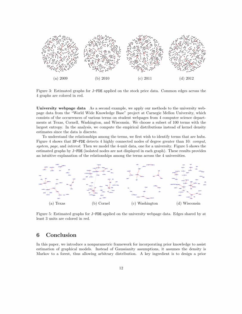
(a) 2009 (b) 2010 (c) 2011 (d) 2012

Figure 3: Estimated graphs for J-FDE applied on the stock price data. Common edges across the4 graphs are colored in red.

University webpage data As a second example, we apply our methods to the university web-page data from the “World Wide Knowledge Base” project at Carnegie Mellon University, whichconsists of the occurrences of various terms on student webpages from 4 computer science depart-ments at Texas, Cornell, Washington, and Wisconsin. We choose a subset of 100 terms with thelargest entropy. In the analysis, we compute the empirical distributions instead of kernel densityestimates since the data is discrete.

To understand the relationships among the terms, we first wish to identify terms that are hubs.Figure 4 shows that SF-FDE detects 4 highly connected nodes of degree greater than 10: comput,system, page, and interest. Then we model the 4-unit data, one for a university. Figure 5 shows theestimated graphs by J-FDE (isolated nodes are not displayed in each graph). These results providesan intuitive explanation of the relationships among the terms across the 4 universities.

comput

scienc

univers

page

home

system

depart

research

interest

work

student

austin

inform

program

link

graduat

web

texa

utexa

address

phone

public

languag

contact

group

parallel

distribut

oper

databas

hall

www

java

graphic

world

algorithm

machin

comput scienc

univers

page

home

system

departresearch

interest

work

student

engin

project

inform

program

link

cornel

web

softwar

languag

network

parallel

distributoper

stuff

school

constructdatabas

design

fall

hall

www

perform

architectur

java

list

graphic

master

high

world site

algorithm

ithaca

internet

applic

thing

friend

area

comput

sciencunivers

page

home

system

depart

research

work

student

engin

program

link

graduat

washington

web

softwar

yearseattl

languag

usa

paper

parallel

distribut

oper

perform

applic

comput

scienc

univers

page

home

system

depart

research

interest

student

enginproject

inform

program

link

offic

graduat

time

madison

web

wisconsin

phone

softwar

public

year

languag

parallel

distribut

person

oper

school

construct

databaseduc

perform

architectur

list

high

world

technolog

algorithm

street

dayton

compil

applic

data

peopl

make

(a) Texas (b) Cornel (c) Washington (d) Wisconsin

Figure 5: Estimated graphs for J-FDE applied on the university webpage data. Edges shared by atleast 3 units are colored in red.

6 Conclusion

In this paper, we introduce a nonparametric framework for incorporating prior knowledge to assistestimation of graphical models. Instead of Gaussianity assumptions, it assumes the density isMarkov to a forest, thus allowing arbitrary distribution. A key ingredient is to design a prior

12

comput

scienc

univers

pagehome

system

depart

research

interest

work

student

engin

austin

project

inform

program

link

offic

cornel

graduat

washington

time

madison

web

texa

utexa

wisconsin address

phone

softwar

email

mail

public

year

seattl

languag

network usapictur

contact

paper

group

parallel

distributresum

person

oper

stuff

school

updat

construct

click

class

databas

design

fallfax

educ

hall

postscript

find

www

perform

architectur

current

java

develop

list

graphic

master

high

modifi

world

site

imag

technologhomepag

algorithm

streetdaytonithaca

internet

compil

applic

check

thing

generdata

info

report

peopl

friend

area

machin

html

support

number

studi

model

make

comput

scienc

univers

page

home

system

depart

research

interest

work

student

engin

austin

project

inform

program

link

offic

cornel

graduat

washington

time

madison

web

texa

utexa

wisconsin

address

phone

softwar

email mail

public

year

seattl

languag

network

usa

pictur

contact

paper

group

parallel

distribut

resum

person

operstuff

school

updat

construct

click

class

databas

design

fall

fax

educ

hall

postscript

find

wwwperform

architectur

currentjava

develop

list

graphic

master

high

modifi

worldsite

imag

technolog

homepag

algorithm

streetdayton

ithaca

internet

compil

applic

check

thing

generdata

info

report peopl

friend

area

machin

html

support

number

studi

model

make

FDE SF-FDE

Figure 4: Estimated graphs for FDE and SF-FDE applied on the university webpage data.

distribution on graphs that favors those consistent with the prior belief. We illustrate the idea byproposing such prior distributions, which lead to two algorithms, for the problems of estimatingscale-free networks and multiple graphs with similar structures. An interesting future direction isto apply this idea to more applications and different types of prior information.

References

[1] Reka Albert and Albert-Laszlo Barabasi. Statistical mechanics of complex networks. Reviewsof Modern Physics, 74(1):47, 2002.

[2] C Chow and C Liu. Approximating discrete probability distributions with dependence trees.Information Theory, IEEE Transactions on, 14(3):462–467, 1968.

[3] Patrick Danaher, Pei Wang, and Daniela M Witten. The joint graphical lasso for inversecovariance estimation across multiple classes. Journal of the Royal Statistical Society: SeriesB (Statistical Methodology), 76(2):373–397, 2014.

[4] Aaron Defazio and Tiberio S Caetano. A convex formulation for learning scale-free networksvia submodular relaxation. In Advances in Neural Information Processing Systems, pages1250–1258, 2012.

[5] Stefano Demarta and Alexander J McNeil. The t copula and related copulas. InternationalStatistical Review, 73(1):111–129, 2005.

[6] Jerome Friedman, Trevor Hastie, and Robert Tibshirani. Sparse inverse covariance estimationwith the graphical lasso. Biostatistics, 9(3):432–441, 2008.

13

[7] Jian Guo, Elizaveta Levina, George Michailidis, and Ji Zhu. Joint estimation of multiplegraphical models. Biometrika, 98(1):1–15, 2011.

[8] David R Hunter and Kenneth Lange. A tutorial on MM algorithms. The American Statistician,58(1):30–37, 2004.

[9] Joseph B Kruskal. On the shortest spanning subtree of a graph and the traveling salesmanproblem. Proceedings of the American Mathematical society, 7(1):48–50, 1956.

[10] Han Liu, Min Xu, Haijie Gu, Anupam Gupta, John Lafferty, and Larry Wasserman. Forestdensity estimation. The Journal of Machine Learning Research, 12:907–951, 2011.

[11] Qiang Liu and Alexander T Ihler. Learning scale free networks by reweighted `1 regularization.In International Conference on Artificial Intelligence and Statistics, pages 40–48, 2011.

[12] Christine Peterson, Francesco C. Stingo, and Marina Vannucci. Bayesian inference of multipleGaussian graphical models. Journal of the American Statistical Association, 110(509):159–174,2015.

[13] Kean Ming Tan, Palma London, Karthik Mohan, Su-In Lee, Maryam Fazel, and DanielaWitten. Learning graphical models with hubs. The Journal of Machine Learning Research, 15(1):3297–3331, 2014.

[14] Qingming Tang, Siqi Sun, and Jinbo Xu. Learning scale-free networks by dynamic node specificdegree prior. In Proceedings of the 32nd International Conference on Machine Learning, pages2247–2255, 2015.

[15] Yuancheng Zhu and Rina Foygel Barber. The log-shift penalty for adaptive estimation ofmultiple Gaussian graphical models. In Proceedings of the 18th International Conference onArtificial Intelligence and Statistics, pages 1153–1161, 2015.

14