IEEE TRANSACTIONS ON AUDIO, SPEECH, AND LANGUAGE PROCESSING, VOL. 15, NO. 8, NOVEMBER 2007 2561

Correspondence

A Pole-Zero Placement Technique for DesigningSecond-Order IIR Parametric Equalizer Filters

Toon van Waterschoot, Student Member, IEEE, andMarc Moonen, Fellow, IEEE

Abstract—A new procedure is presented for designing second-orderparametric equalizer filters. In contrast to the traditional approach, inwhich the design is based on a bilinear transform of an analog filter, thepresented procedure allows for designing the filter directly in the digitaldomain. A rather intuitive technique known as pole-zero placement, istreated here in a quantitative way. It is shown that by making somemeaningful approximations, a set of relatively simple design equationscan be obtained. Design examples of both notch and resonance filters areincluded to illustrate the performance of the proposed method and tocompare with state-of-the-art solutions.

Index Terms—Filter design, notch filters, parametric equalizer filters,pole-zero placement, resonance filters.

I. INTRODUCTION

Many signal processing applications involve enhancing or atten-uating only a small portion of a signal’s frequency spectrum, whileleaving the remainder of the spectrum unaffected. This effect isobtained by using bandpass or bandstop filters that have a frequencyresponse which is characterized by a gain increase or decrease arounda specified center frequency fc. In digital audio equalization, anydesired frequency response may be realized by cascading such band-pass/-stop filters with different center frequencies, which are thenoften referred to as parametric equalizer filters or presence filters. Sucha cascade may moreover include high-pass and low-pass filters, alsoknown as shelving filters, which are in fact special (degenerate) casesof the bandpass/-stop filter, having one real pole-zero pair instead oftwo complex conjugate pole-zero pairs.

Apart from the center frequency, a parametric equalizer filter is alsocharacterized by its bandwidth (which we will define later on). Filtershaving a small bandwidth B relative to their center frequency (i.e.,having a high Q-factor, defined as Q = fc=B), are better known asnotch and resonance (or peaking) filters. Notch filters appear in nu-merous applications where a (nearly) sinusoidal interference has to becanceled from a broadband signal, e.g., suppressing a 50/60 Hz ac in-terference in a low-voltage measurement signal, or canceling acousticfeedback oscillations in audio amplification systems. Resonance filters

Manuscript received January 22, 2007; revised June 21, 2007. This work wassupported by the Institute for the Promotion of Innovation through Science andTechnology in Flanders (IWT-Vlaanderen) and carried out at the ESAT Labo-ratory of the Katholieke Universiteit Leuven, in the frame of K.U.Leuven Re-search Council: CoE EF/05/006 Optimization in Engineering (OPTEC), the Bel-gian Programme on Interuniversity Attraction Poles, initiated by the BelgianFederal Science Policy Office IUAP P6/04 (DYSCO, “Dynamical systems, con-trol, and optimization,” 2007-2011), the Concerted Research Action GOA-AM-BioRICS, and IWT project 040803: “SMS4PA-II: Sound Management Systemfor Public Address Systems.” The scientific responsibility is assumed by its au-thors. The associate editor coordinating the review of this paper and approvingit for publication was Dr. Helen M. Meng.

The authors are with the Department of Electrical Engineering, ESAT-SCD,Katholieke Universiteit Leuven, B-3001 Leuven, Belgium (e-mail: toon.vanwa-terschoot@esat.kuleuven.be; marc.moonen@esat.kuleuven.be).

Digital Object Identifier 10.1109/TASL.2007.905180

are typically used to recover sinusoids buried in noise (so-called lineenhancement), e.g., in communications and sonar applications.

It is well known that a bandpass or bandstop characteristic around aspecified center frequency can be realized efficiently using a second-order infinite impulse response (IIR) filter [1]–[11], also known as abiquadratic filter, with transfer function

H(z) =b0 + b1z

�1 + b2z�2

1 + a1z�1 + a2z�2: (1)

Traditionally, the five filter coefficients are calculated so as to satisfy aset of five design equations [7]:

jH(ej0)j =G0 (gain at dc) (2a)

jH(ej�)j =G� (gain at Nyquist frequency)

(2b)@

@!jH(ej!)j !=! =0 (center frequency) (2c)

jH(ej! )j =Gc (gain at resonance) (2d)

jH(ej(! �B=2))j =GB (bandwidth) (2e)

where ! = 2�f represents radial frequency. These design equationsincorporate the following design variables: (radial) center frequency!c, (radial) bandwidth B, gain at band edges GB , gain at resonanceGc, gain at dc G0, and gain at Nyquist frequency G� . Typically, the dcand Nyquist gain are chosen to be equal (except in [10], with the aim ofdigitally emulating an analog equalizer) and are set to 0 dB, i.e., G0 =G� = 1, which facilitates the cascading of several parametric equalizerfilters. Unfortunately, there is little agreement in the literature on how toappropriately define bandwidth [7]. We will adopt Moorer’s bandwidthdefinition [2], which is found to be mathematically the most consistentone [7]. If the resonance gain relative to the gain at dc, i.e., Gc=G0

(called the “boost” in a resonance filter and the “cut” in a notch filter),exceeds 6 dB in absolute value, then the band edges are defined as thefrequencies at which the gain is 3 dB below/above the peak/notch. Fora boost/cut less than 6 dB in absolute value, the band edges are foundat the so-called midpoint gain, which is defined as the geometric meanpGcG0, i.e., 1=2(Gc;dB �G0;dB) dB below/above the peak/notch.Nearly all existing design procedures start from the design of an

analog parametric equalizer filter, followed by a bilinear transform thatmaps the analog frequency axis [0;1) onto the digital frequency axis[0; fs=2], with fs the sampling frequency [1], [3]–[7], [10]. To thisend, the digital design variables !c and B should be “prewarped” toanalog variables, which can, however, not be done in an exact way forthe bandwidth [5], [7]. As an alternative, the parametric equalizer filtercan also be designed directly in the digital domain. A first approachwas suggested in [2] and starts by designing a digital parametric equal-izer filter with center frequency !c = �=2 (which is the only digitalcenter frequency that allows for a truly symmetric frequency response,leading to b1 = a1 = 0). The filter centered at �=2 is then transformedto an arbitrarily centered filter using an appropriate bilinear transform.A second approach is more intuitive and based on a technique knownas pole-zero placement. It was shown earlier how a resonance filterwith a specified center frequency and bandwidth can be designed inthe z-plane by placing two complex conjugate poles (inside, but closeto the unit circle) on the radial lines from the origin to e�j! , and twozeros at the origin [8, Ch. 6], [9, Ch. 6], [11, Ch. 11]. For this designprocedure, several approximate relations between the bandwidth andthe so-called pole radius (i.e., the distance from the origin to the pole)

1558-7916/$25.00 © 2007 IEEE

2562 IEEE TRANSACTIONS ON AUDIO, SPEECH, AND LANGUAGE PROCESSING, VOL. 15, NO. 8, NOVEMBER 2007

have been suggested [8, Ch. 6], [11, Ch. 11]. Also, it was noted in [9,Ch. 6], that by moving the zeros from the origin towards the poles, andeven beyond, the resonance characteristic can be converted into a notchcharacteristic.

The aim of this correspondence is to present a more quantitativetreatment of the pole-zero placement approach. We will derive exactrelations between the pole and zero positions on the one hand, and thedesign variables on the other hand. These relations will, however, ap-pear to be impractical for implementation, and hence we will suggestsome useful approximations. The pole-zero placement design proce-dure is outlined in Section II, where we will make a distinction be-tween notch filter and resonance filter design. Some design examplesare given in Section III, and finally, Section IV concludes this corre-spondence.

II. DESIGN PROCEDURE

The pole-zero placement design procedure is based on a radial repre-sentation of the biquadratic filter transfer function, in which poles andzeros are constrained to lie on the radial lines from the origin to e�j!

[9, Ch. 6], [11, Ch. 11], [12], i.e.,

H(z) = K (1�r e z )(1�r e z )

(1�r e z )(1�r e z )(3)

which can equivalently be written in direct form as

H(z) = K1� 2rz cos!cz

�1 + r2zz�2

1� 2rp cos!cz�1 + r2pz�2: (4)

The zero radius rz 2 [0; 1] is defined as the distance from the originto each of the complex conjugate zeros, and likewise the pole radiusrp 2 [0; 1) is defined as the distance from the origin to the poles. Abroadband gain factor K is also included.

In contrast to the original biquadratic filter transfer function in (1),the radial representation contains only four distinct parameters and, asa consequence, only four design equations can be fulfilled. Therefore,the design equations (2a) and (2b) may be replaced by only one equa-tion that specifies the filter response at an arbitrary frequency. For con-venience, however, we will just omit (2b) and retain (2a). Furthermore,since the center frequency can be specified directly in the radial rep-resentation in (3) or (4), design equations (2c) can also be omitted.Note that (2c) would, however, only be exactly fulfilled for a desiredcenter frequency at !c = f0; �=2; �g, since the maximum/minimumin the frequency response of the constrained resonance/notch filter in(3) does not generally appear at the resonance frequency, which is dueto the influence of the complex conjugate pole-zero pair [11, Ch. 11].This effect decreases as the poles approach the unit circle.

We will now derive exact and approximate relations between the re-maining three filter parameters frz ; rp; Kg and the design variablesf!c; B;G0; Gcg, by evaluating the remaining design equations (2a),(2d), and (2e). We will generally assume that the poles are close tothe unit circle, i.e., 0 � rp < 1, resulting in narrowband parametricequalizer filters. To obtain a broader bandpass/bandstop characteristic,a cascade of shelving filters should be used instead. Below, the designof notch and resonance filters is treated separately, since different as-sumptions can be made in either case.

A. Notch Filters

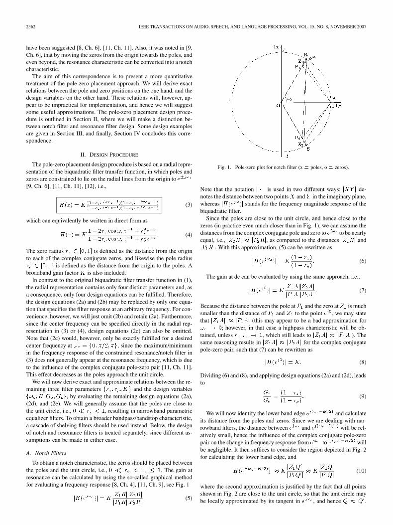
To obtain a notch characteristic, the zeros should be placed betweenthe poles and the unit circle, i.e., 0 � rp < rz � 1. The gain atresonance can be calculated by using the so-called graphical methodfor evaluating a frequency response [8, Ch. 4], [11, Ch. 9], see Fig. 1

jH(ej! )j = KjZ1RjjZ2Rj

jP1RjjP2Rj: (5)

Fig. 1. Pole-zero plot for notch filter (x = poles, o = zeros).

Note that the notation j � j is used in two different ways: jXY j de-notes the distance between two pointsX and Y in the imaginary plane,whereas jH(ej!)j stands for the frequency magnitude response of thebiquadratic filter.

Since the poles are close to the unit circle, and hence close to thezeros (in practice even much closer than in Fig. 1), we can assume thedistances from the complex conjugate pole and zero to ej! to be nearlyequal, i.e., jZ2Rj � jP2Rj, as compared to the distances jZ1Rj andjP1Rj. With this approximation, (5) can be rewritten as

jH(ej! )j = K(1� rz)

(1� rp): (6)

The gain at dc can be evaluated by using the same approach, i.e.,

jH(ej0)j = KjZ1AjjZ2Aj

jP1AjjP2Aj: (7)

Because the distance between the pole at P1 and the zero at Z1 is muchsmaller than the distance of P1 and Z1 to the point ej0, we may statethat jZ1Aj � jP1Aj (this may appear to be a bad approximation for!c ! 0; however, in that case a highpass characteristic will be ob-tained, unless rp; rz ! 1, which still leads to jZ1Aj � jP1Aj). Thesame reasoning results in jZ2Aj � jP2Aj for the complex conjugatepole-zero pair, such that (7) can be rewritten as

jH(ej0)j = K: (8)

Dividing (6) and (8), and applying design equations (2a) and (2d), leadsto

Gc

G0=

(1� rz)

(1� rp): (9)

We will now identify the lower band edge ej(! �B=2) and calculateits distance from the poles and zeros. Since we are dealing with nar-rowband filters, the distance between ej! and ej(! �B=2) will be rel-atively small, hence the influence of the complex conjugate pole-zeropair on the change in frequency response from ej! to ej(! �B=2) willbe negligible. It then suffices to consider the region depicted in Fig. 2for calculating the lower band edge, and

jH(ej(! �B=2))j � KjZ1Q

0j

jP1Q0j� K

jZ1Qj

jP1Qj(10)

where the second approximation is justified by the fact that all pointsshown in Fig. 2 are close to the unit circle, so that the unit circle maybe locally approximated by its tangent in ej! , and hence Q � Q0.

IEEE TRANSACTIONS ON AUDIO, SPEECH, AND LANGUAGE PROCESSING, VOL. 15, NO. 8, NOVEMBER 2007 2563

Fig. 2. Bandwidth calculation for notch filter.

Furthermore, the arc length betweenR andQ0 is nearly equal to jRQj.Since the frequency response is approximately symmetric around thecenter frequency if the poles are close to the unit circle [11, Ch. 11],the bandwidth can be calculated as B � 2jRQj.

Recall our definition of bandwidth

jH(ej! )jjH(ej(! �B=2))j =

1p2; if G

G� 1

2

GG; if G

G� 1

2.

(11)

Moreover, combining (6) and (10) yields

jH(ej! )jjH(ej(! �B=2))j =

(1� rz)jP1Qj(1� rp)jZ1Qj : (12)

With the Pythagorean theorem applied to the triangles P1RQ andZ1RQ, we obtain two more equations

jP1Qj2 = jP1Rj2 + jRQj2 = (1� rp)2 + jRQj2 (13)

jZ1Qj2 = jZ1Rj2 + jRQj2 = (1� rz)2 + jRQj2 (14)

which can be solved for jRQj, together with (11) and (12), resulting in

B � 2jRQj =2

(1�r ) (1�r )

(1�r ) �2(1�r ); if G

G� 1

2

2( �1)(1�r ) (1�r )

(1�r ) � (1�r ); if G

G� 1

2.

(15)

Dividing both the numerator and denominator in the above square rootexpressions by either (1� rp)

2 or (1� rz)2, and subsequently using

the result in (9), yields the following expressions for the zero and poleradius

rz =1� B

21� 2

G

G; if G

G� 1

2

1� B2

GG; if G

G� 1

2

(16)

rp =1� B

2

G

G� 2; if G

G� 1

2

1� B2

GG; if G

G� 1

2:

(17)

These expressions, together withK = G0 , constitute the notch filter

design procedure. Note that, while the expressions in (16) and (17)may theoretically yield negative results, this should never occur for thenarrowband filters we are dealing with (i.e., for sufficiently small B).

B. Resonance Filters

A similar procedure can be used to design resonance filters, but thenthe zeros should be placed between the origin and the poles, i.e., 0 �rz < rp < 1; see Fig. 3. Note that in this case, no assumption can bemade about the position of the zeros, i.e., depending on the specifiedgain at resonance, the zeros may be close to the origin, or close to the

Fig. 3. Pole-zero plot for resonance filter.

Fig. 4. Bandwidth calculation for resonance filter.

poles (near the unit circle), or anywhere in between. We will howeverassume that the distance between Z1 and P1 is significantly larger thanthe distance from P1 to the unit circle, and the same for Z2 and P2,such that the zeros can be neglected when calculating the bandwidth.As in the notch filter case, we will also assume that the influence of thecomplex conjugate pole-zero pair on the change in frequency responsefrom ej! to ej(! �B=2) is negligible. Hence, the bandwidth, which inthis case is defined by

jH(ej! )jjH(ej(! �B=2))j =

p2; if G

G� 2

GG; if G

G� 2

(18)

only depends on the pole position, see Fig. 4, i.e.,

jH(ej! )jjH(ej(! �B=2))j �

jP1Qj(1� rp)

: (19)

This expression, together with the Pythagorean theorem in (13), resultsin

B � 2jRQj =2(1� rp); if G

G� 2

2(1� rp)GG� 1; if G

G� 2

(20)

so that the pole radius can be calculated as

rp =

1� B2; if G

G� 2

1� B

2 �1

; if GG

� 2. (21)

The upper part of (21) was also derived in [8, Ch. 6].Determining the zero radius for the resonance filter is somewhat

more difficult, as no assumption can be made about the position of the

2564 IEEE TRANSACTIONS ON AUDIO, SPEECH, AND LANGUAGE PROCESSING, VOL. 15, NO. 8, NOVEMBER 2007

zeros. Graphically evaluating the gain at resonance and at dc yields

jH(ej! )j =K(1� rz)jZ2Rj(1� rp)jP2Rj (22)

jH(ej0)j =KjZ1AjjZ2AjjP1AjjP2Aj = K

jZ1Aj2jP1Aj2 : (23)

Eliminating K from (22) and (23), and taking into account design (2a)and (2d), leads to

(1� rz)jZ2RjjP1Aj2(1� rp)jP2RjjZ1Aj2 =

Gc

G0

(24)

where we can make the following approximations. Since the poles areclose to the unit circle, jP2Rj � jSRj = 2 sin!c, and jP1Aj �jRAj = 2(1� cos!c). Furthermore, the fraction

jZ1Aj2jZ2Rj =

r2z � 2rz cos!c + 1pr2z � 2rz cos 2!c + 1

(25)

may be approximated by a first-order polynomial in rz . As rz variesbetween 0 and 1, the fraction in (25) takes on a value between 1 and(1� cos!c)= sin!c, which leads to the following approximation:

jZ1Aj2jZ2Rj � (1� rz) +

1� cos!csin!c

rz : (26)

Substituting the above approximations in (24), results in a first-orderequation in rz

(1� rz)

(1� rp)=Gc

G0

rz + (1� rz)sin!c

1� cos!c(27)

which can readily be solved by using (21), i.e.,

rz =

1��

1��+; if G

G� 2

1��

1��+; if G

G� 2 (28)

with

� =

B

2

G

G

sin!

1�cos!; if G

G� 2

B

2 �1

G

G

sin!

1�cos!; if G

G� 2. (29)

It should be noted that, once the bandwidth is specified, the boostGc=G0 cannot take on an arbitrarily large value. The maximum boost,given B, is obtained when the zeros are placed at the origin, and canbe calculated from (29) with � = 1.

Finally, the broadband gain factorK can be calculated by evaluating(4) at ej0, i.e.,

K = G0

1�2r cos! +r

1�2r cos! +r: (30)

III. DESIGN EXAMPLES

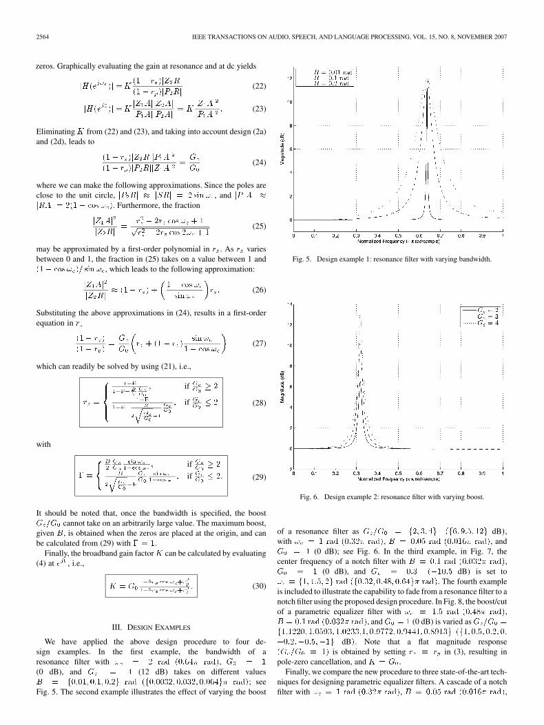
We have applied the above design procedure to four de-sign examples. In the first example, the bandwidth of aresonance filter with !c = 2 rad (0:64� rad), G0 = 1(0 dB), and Gc = 4 (12 dB) takes on different valuesB = f0:01; 0:1; 0:2g rad (f0:0032; 0:032; 0:064g� rad); seeFig. 5. The second example illustrates the effect of varying the boost

Fig. 5. Design example 1: resonance filter with varying bandwidth.

Fig. 6. Design example 2: resonance filter with varying boost.

of a resonance filter as Gc=G0 = f2; 3; 4g (f6; 9:5; 12g dB),with !c = 1 rad (0:32� rad), B = 0:05 rad (0:016� rad), andG0 = 1 (0 dB); see Fig. 6. In the third example, in Fig. 7, thecenter frequency of a notch filter with B = 0:1 rad (0:032� rad),G0 = 1 (0 dB), and Gc = 0:3 (�10:5 dB) is set to!c = f1; 1:5; 2g rad (f0:32;0:48; 0:64g� rad). The fourth exampleis included to illustrate the capability to fade from a resonance filter to anotch filter using the proposed design procedure. In Fig. 8, the boost/cutof a parametric equalizer filter with !c = 1:5 rad (0:48� rad),B = 0:1 rad (0:032� rad), and G0 = 1 (0 dB) is varied as Gc=G0 =f1:1220;1:0593;1:0233;1;0:9772;0:9441;0:8913g (f1; 0:5; 0:2; 0;�0:2;�0:5;�1g dB). Note that a flat magnitude response(Gc=G0 = 1) is obtained by setting rz = rp in (3), resulting inpole-zero cancellation, and K = G0.

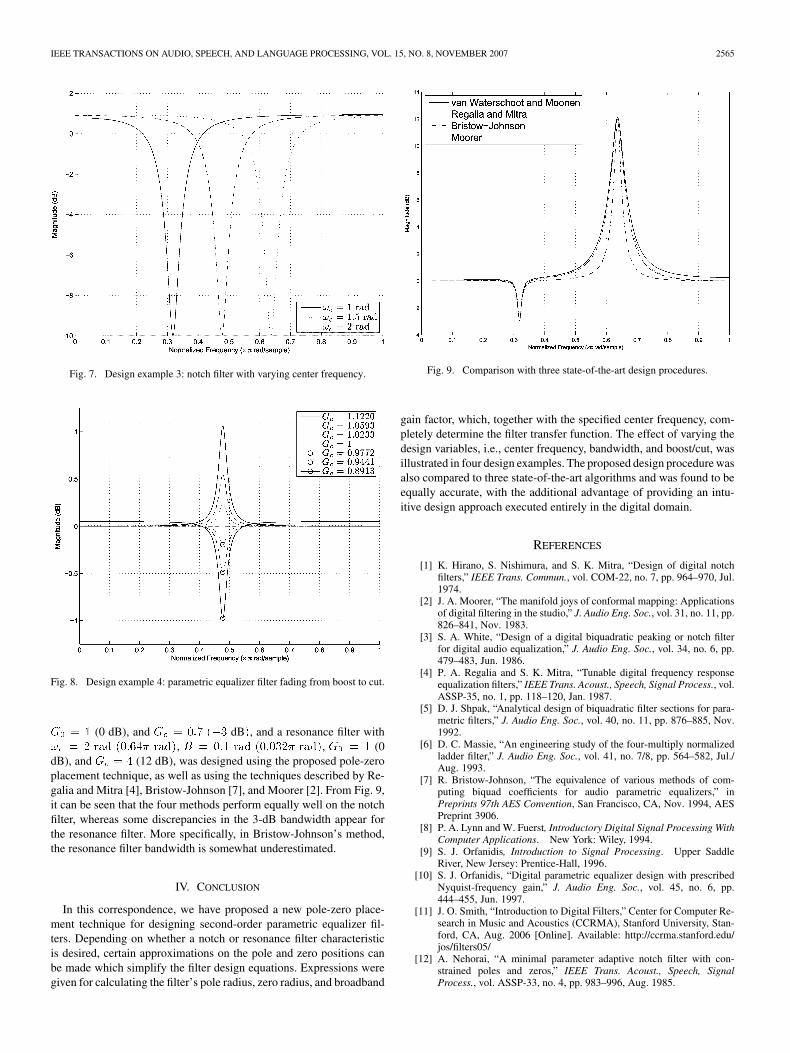
Finally, we compare the new procedure to three state-of-the-art tech-niques for designing parametric equalizer filters. A cascade of a notchfilter with !c = 1 rad (0:32� rad), B = 0:05 rad (0:016� rad),

IEEE TRANSACTIONS ON AUDIO, SPEECH, AND LANGUAGE PROCESSING, VOL. 15, NO. 8, NOVEMBER 2007 2565

Fig. 7. Design example 3: notch filter with varying center frequency.

Fig. 8. Design example 4: parametric equalizer filter fading from boost to cut.

G0 = 1 (0 dB), and Gc = 0:7 (�3 dB), and a resonance filter with!c = 2 rad (0:64� rad), B = 0:1 rad (0:032� rad), G0 = 1 (0dB), and Gc = 4 (12 dB), was designed using the proposed pole-zeroplacement technique, as well as using the techniques described by Re-galia and Mitra [4], Bristow-Johnson [7], and Moorer [2]. From Fig. 9,it can be seen that the four methods perform equally well on the notchfilter, whereas some discrepancies in the 3-dB bandwidth appear forthe resonance filter. More specifically, in Bristow-Johnson’s method,the resonance filter bandwidth is somewhat underestimated.

IV. CONCLUSION

In this correspondence, we have proposed a new pole-zero place-ment technique for designing second-order parametric equalizer fil-ters. Depending on whether a notch or resonance filter characteristicis desired, certain approximations on the pole and zero positions canbe made which simplify the filter design equations. Expressions weregiven for calculating the filter’s pole radius, zero radius, and broadband

Fig. 9. Comparison with three state-of-the-art design procedures.

gain factor, which, together with the specified center frequency, com-pletely determine the filter transfer function. The effect of varying thedesign variables, i.e., center frequency, bandwidth, and boost/cut, wasillustrated in four design examples. The proposed design procedure wasalso compared to three state-of-the-art algorithms and was found to beequally accurate, with the additional advantage of providing an intu-itive design approach executed entirely in the digital domain.

REFERENCES

[1] K. Hirano, S. Nishimura, and S. K. Mitra, “Design of digital notchfilters,” IEEE Trans. Commun., vol. COM-22, no. 7, pp. 964–970, Jul.1974.

[2] J. A. Moorer, “The manifold joys of conformal mapping: Applicationsof digital filtering in the studio,” J. Audio Eng. Soc., vol. 31, no. 11, pp.826–841, Nov. 1983.

[3] S. A. White, “Design of a digital biquadratic peaking or notch filterfor digital audio equalization,” J. Audio Eng. Soc., vol. 34, no. 6, pp.479–483, Jun. 1986.

[4] P. A. Regalia and S. K. Mitra, “Tunable digital frequency responseequalization filters,” IEEE Trans. Acoust., Speech, Signal Process., vol.ASSP-35, no. 1, pp. 118–120, Jan. 1987.

[5] D. J. Shpak, “Analytical design of biquadratic filter sections for para-metric filters,” J. Audio Eng. Soc., vol. 40, no. 11, pp. 876–885, Nov.1992.

[6] D. C. Massie, “An engineering study of the four-multiply normalizedladder filter,” J. Audio Eng. Soc., vol. 41, no. 7/8, pp. 564–582, Jul./Aug. 1993.

[7] R. Bristow-Johnson, “The equivalence of various methods of com-puting biquad coefficients for audio parametric equalizers,” inPreprints 97th AES Convention, San Francisco, CA, Nov. 1994, AESPreprint 3906.

[8] P. A. Lynn and W. Fuerst, Introductory Digital Signal Processing WithComputer Applications. New York: Wiley, 1994.

[9] S. J. Orfanidis, Introduction to Signal Processing. Upper SaddleRiver, New Jersey: Prentice-Hall, 1996.

[10] S. J. Orfanidis, “Digital parametric equalizer design with prescribedNyquist-frequency gain,” J. Audio Eng. Soc., vol. 45, no. 6, pp.444–455, Jun. 1997.

[11] J. O. Smith, “Introduction to Digital Filters,” Center for Computer Re-search in Music and Acoustics (CCRMA), Stanford University, Stan-ford, CA, Aug. 2006 [Online]. Available: http://ccrma.stanford.edu/jos/filters05/

[12] A. Nehorai, “A minimal parameter adaptive notch filter with con-strained poles and zeros,” IEEE Trans. Acoust., Speech, SignalProcess., vol. ASSP-33, no. 4, pp. 983–996, Aug. 1985.