zef-discussion papers on development policy no....
TRANSCRIPT

ZEF-Discussion Papers on Development Policy No. 186
Vijesh Krishna, Matin Qaim and David Zilberman
Transgenic Crops, Production Risk, and Agrobiodiversity
Bonn, February 2014

The CENTER FOR DEVELOPMENT RESEARCH (ZEF) was established in 1995 as an international, interdisciplinary research institute at the University of Bonn. Research and teaching at ZEF addresses political, economic and ecological development problems. ZEF closely cooperates with national and international partners in research and development organizations. For information, see: www.zef.de. ZEF – Discussion Papers on Development Policy are intended to stimulate discussion among researchers, practitioners and policy makers on current and emerging development issues. Each paper has been exposed to an internal discussion within the Center for Development Research (ZEF) and an external review. The papers mostly reflect work in progress. The Editorial Committee of the ZEF – DISCUSSION PAPERS ON DEVELOPMENT POLICY include Joachim von Braun (Chair), Solvey Gerke, and Manfred Denich. Tobias Wünscher is Managing Editor of the series.
Vijesh Krishna, Matin Qaim and David Zilberman, Transgenic Crops, Production Risk, and Agrobiodiversity, ZEF- Discussion Papers on Development Policy No. 186, Center for Development Research, Bonn, February 2014, pp.32. ISSN: 1436-9931 Published by: Zentrum für Entwicklungsforschung (ZEF) Center for Development Research Walter-Flex-Straße 3 D – 53113 Bonn Germany Phone: +49-228-73-1861 Fax: +49-228-73-1869 E-Mail: [email protected] www.zef.de The authors: Vijesh Krishna, Department of Agricultural Economics and Rural Development, Georg-August-University of Goettingen. Contact: [email protected] Matin Qaim, Department of Agricultural Economics and Rural Development, Georg-August-University of Goettingen. Contact: [email protected] David Zilberman, Department of Agricultural and Resource Economics, University of California, Berkeley. Contact: [email protected]

Acknowledgements
This study was financially co-supported by the German Research Foundation (DFG), the German Federal Ministry of Economic Cooperation and Development (BMZ) and the European Commission (EC).
Abstract
Do transgenic crops cause agrobiodiversity erosion? We hypothesize that they increase productivity and reduce production risk and may therefore reduce farmer demand for on-farm varietal diversity, especially when only a few transgenic varieties are available. We also hypothesize that varietal diversity can be preserved when more transgenic varieties are supplied. These hypotheses are tested and confirmed with panel data for the case of transgenic cotton in India. Cotton varietal diversity in India, with of over 90% adoption of transgenic technology, is now at the same level than it was before the introduction of this technology. Some policy implications are discussed.
Keywords: varietal diversity, biotechnology, smallholder farmers, production risk, India
JEL classification: D24, D81, O13, O44, Q12, Q16, Q57
1
1. Introduction
This study analyzes the impact of transgenic crop adoption on agricultural production risk
and agrobiodiversity. The genetic erosion hypothesis suggests that global biodiversity is
affected by various anthropogenic stresses (Van Straalen and Timmermans, 2002) that have
caused serious biodiversity loss over the past few decades (Millennium Ecosystem
Assessment, 2005). This also applies to agrobiodiversity, comprising the diversity of species
used in agricultural production and varietal diversity within those species. One of the major
factors that have influenced agrobiodiversity over the last 100 years is plant breeding,
coupled with the intensification of agricultural systems. Farmer adoption of a few genetically
uniform high-yielding varieties (HYVs) has the potential to erode landraces and reduce the
diversity of indigenous crop varieties (Harlan, 1975; Brush, 2000). Modern high-yielding
varieties may be attractive for farmers from a short-term profit maximizing perspective, but
it is argued that a narrower genetic base may increase production risk and disrupt the
stability and resilience of farming systems in the long run (Cooper, Engels and Frison, 1994;
Tripp, 1996). Indeed, there is broad evidence that varietal diversity has a natural insurance
function (Baumgärtner and Quaas, 2010; Di Falco and Chavas, 2009). Against this
background, some argue that the Green Revolution (i.e., the introduction of HYVs of wheat
and rice since the late 1960s in Asia and other parts of the developing world) has
contributed to serious ecological and social problems in the small farm sector (Shiva 1991).1
And there are widespread concerns that the loss of agrobiodiversity may be further
exacerbated through the introduction of new breeding technologies, such as transgenic
crops (Holt-Gimenez and Altieri, 2013).
Several recent studies have analyzed the impact of transgenic crops on agricultural
productivity and income, concluding that farmers can benefit significantly from adopting
these crops (Qaim, 2009; Carpenter, 2010). This also applies to smallholder farmers in
developing countries (Crost et al., 2007; Huang et al., 2010; Subramanian and Qaim, 2010;
Qaim and Kouser, 2013). There are also studies that have analyzed potential biodiversity
impacts occurring through outcrossing of transgenes into wild relatives of domesticated
1 Smale (1997) showed that the negative impacts of the Green Revolution on agrobiodiversity are actually
smaller than often assumed.
2
crops (Bellon and Berthaud, 2004; Raven, 2010). While certain risks for biodiversity exist,
Raven (2010) concludes that these do not differ between transgenic and conventionally bred
crops. However, to the best of our knowledge, the impact of transgenic technology on the
diversity of crop varieties grown by farmers has never been studied empirically in developing
countries.2
There are at least three aspects that make transgenic crops different from HYVs of the Green
Revolution, so previous results on the impact of breeding technologies on varietal diversity
cannot simply be extrapolated. First, many transgenic technologies involve crop resistance
to biotic and abiotic stress factors. Thus, transgenic crops may not only be higher yielding
but also risk reducing (Crost and Shankar, 2008). Adoption of stress-resistant transgenic
crops may reduce demand for the insurance function of agrobiodiversity, potentially
resulting in accelerated loss of varietal diversity. Second, the product of transgenic breeding
is not only one single new crop variety. Rather, transgenic technology allows the
introduction of desirable genes and traits into many existing varieties. Thus, it may be easier
to preserve varietal diversity (Zilberman, Ameden and Qaim, 2007). Third, transgenic crops
are primarily commercialized by private companies, and they are also associated with new
regulations, including intellectual property rights (IPRs) and complex biosafety approval
procedures. Such institutional factors may also influence the technology’s impacts on
varietal diversity (Qaim, Yarkin, Zilberman, 2005).
Here, we use data from the Indian cotton sector to analyze linkages between transgenic
technology, production risk, institutional factors, and varietal diversity. Transgenic cotton
with inbuilt insect resistance was first commercialized in India in 2002. Since then, it has
been adopted by several million smallholder farmers on over 90% of the national cotton
area (James, 2012). We use four rounds of panel data that we collected between 2002 and
2008. Hence, we capture the early diffusion phase of transgenic cotton in India with
relatively low adoption, as well as later diffusion phases with high adoption rates. The data
also provide a quasi-experimental setting for the analysis of interesting institutional and
policy aspects. In the first few years of technology diffusion, only a small number of
transgenic cotton varieties had received approval by the national biosafety authorities.
2 In an ex ante study, Kolady and Lesser (2012) have analyzed the possible effects of transgenic eggplant
technology on varietal diversity in India, but this technology was not yet commercially released in the country, so that ex post data are not available.

3
Hence, only these few approved transgenic varieties were supplied in the seed market,
alongside a much larger number of conventional cotton varieties (Qaim et al., 2006; Smale et
al., 2009). In later years, additional transgenic varieties were approved and marketed by
several seed companies. Since 2006, the number of transgenic varieties supplied in the
market has increased manifold (Tripp, 2009; Choudhary and Gaur, 2010).
The remaining part of this paper is organized as follows. In the next section, we develop a
conceptual framework and derive concrete research hypotheses. Details of the situation in
India and the data collected from cotton farms are presented in section 3. In section 4, we
describe the empirical methods, and in section 5 we present and discuss the estimation
results. Section 6 concludes with some broader policy implications.
2. Conceptual Framework and Research Hypotheses
In traditional farming with little impact of modern technology, smallholders often grow
several varieties of the same crop, that is, they have a relatively high level of on-farm varietal
diversity. Such diversity is associated with societal benefits, because the option value of a
broad base of plant genetic resources is preserved (Smale, 2006). But on-farm varietal
diversity also has private benefit components. One can discern two possible functions that
varietal diversity may offer to farmers, first, an insurance function, and second, a
productivity enhancement function (Di Falco and Chavas, 2009).
The insurance function is related to production risks due to pests, diseases, and erratic
weather conditions. Different varieties have different levels of susceptibility to such stresses;
hence growing several varieties tends to reduce covariate risks. In this situation, when a new
HYV is introduced it may be adopted only partially, especially in the absence of formal
insurance markets (Baumgärtner and Quaas, 2010). Farmers who seek to avoid downside
income risk may choose to include lower-productive but less-vulnerable traditional varieties
in their varietal portfolio, even though full adoption of the HYV might be more profitable on
average (Smale, Just and Leathers, 1994). The productivity enhancement function of varietal
diversity implies that growing several varieties on the same farm may also increase mean
yield levels, which may be due to complementarity or scale effects (Chavas and Di Falco,
2012; Boreux et al., 2013). Complementarity effects occur in a production system when
4
particular varieties perform better in the presence of others, for instance through lower
infestation levels of certain pests or diseases. Scale effects arise when the functioning of the
system is affected by its degree of fragmentation. Different plots on the same farm may
differ in soil type, slope, and other characteristics, so that crop performance may be
increased when varieties that are optimally suited for each plot are cultivated. Again, a new
HYV that is not optimally suited for all plots may be adopted only partially, especially when
plot heterogeneity is significant.
What will happen to on-farm varietal diversity when a new transgenic crop is introduced?
The answer to this question will depend on the importance of the insurance and productivity
enhancement functions of diversity in the initial situation, and on the concrete transgenic
trait that is newly introduced. Most transgenic crop technologies available so far involve
insect resistance, virus resistance, or herbicide tolerance (James, 2012). Other transgenic
traits that are in the research pipeline include fungal and bacterial resistance, and tolerance
to drought, heat, and other abiotic stresses (Qaim, 2009). Hence, the new transgenic crop is
likely to reduce production risk. At the same time, it is likely to increase yield, not necessarily
through higher yield potential but through more effective damage control (Qaim and
Zilberman, 2003). We will start the analysis with the following general hypothesis:
Hypothesis I: Transgenic technology adoption increases yield and reduces production risk
If this hypothesis is true, the transgenic crop technology may potentially substitute for both
the productivity enhancement function and the insurance function of varietal diversity. Most
of the currently available transgenic crops address only single stress factors, so the degree of
substitution will depend on the importance of the particular stress factor and of other stress
factors in the local setting. Moreover, it will depend on the local suitability of crop varieties
into which the transgenic trait is being introduced. For developing concrete hypotheses on
the impacts of transgenic technology on varietal diversity, we use two stylized conceptual
models – the first focusing on the productivity enhancement function and the second one
addressing the insurance function of agrobiodiversity.
We consider the case of a farmer who operates on a given area of land and decides whether
to adopt the transgenic technology and what level of varietal diversity to maintain across
different plots in order to maximize farm income. This model builds on Smale, Just and

5
Leathers (1994), Van Dusen and Taylor (2005), and Krishna et al. (2013), who explored
farmer adoption of different crop varieties with varying degrees of adaptability to different
plots on a given farm, yet without considering transgenic technology. The model is
graphically represented in Figure 1. For simplicity, we assume that the farm only has two
plots (plots a and b) that differ in terms of soil type and other characteristics, although the
scenario can be easily extended to a farm with multiple plots. The horizontal axis shows the
land area of the two plots, and the vertical axes show marginal productivity of a single
output produced. Different crop varieties will lead to different yields on the two plots. Other
factors and inputs are used in the production process, but these are held fixed, so that
marginal productivity is diminishing with increasing plot size. As a starting point, the farmer
grows conventional variety 1 (CV1) on plot a. The same variety could also be grown on plot
b, but its productivity would be significantly lower, because CV1 is not optimally adapted to
the soil and other conditions of plot b. Conventional variety 2 (CV2) is better suited to these
conditions and leads to higher productivity. Hence, total production is higher when the
farmer cultivates two varieties instead of monoculture of CV1 on both plots.
Figure 1: Potential impact of transgenic technology on crop productivity and varietal
diversity on a farm with heterogeneous plots
plot a
Marginal productivity
(plot a)
Marginal productivity
(plot b)
CV1
CV1
TV1
TV1
CV2TV2
plot b

6
Now we consider that a new transgenic trait (e.g., insect resistance) becomes available and
is introduced in variety 1; hence a transgenic version of variety 1 (TV1) is sold in the seed
market. Figure 1 shows that TV1 will lead to a higher productivity than CV1, due to more
effective pest control and thus lower crop damage. The farmer is likely to adopt TV1 on plot
a. The farmer may also adopt TV1 on plot b and thus replace CV2, if the productivity gain
from the transgenic trait is larger than the productivity loss from using a variety that is
otherwise not optimally adapted to the conditions of plot b. In Figure 1, such replacement
would occur if triangle area 𝑥ʹ𝑦ʹ𝑧 is larger than triangle area 𝑥𝑦𝑧. In that case, on-farm
varietal diversity would be reduced. The probability of such diversity erosion would be much
lower if the transgenic trait were also introduced in variety 2, so that transgenic versions of
both varieties (TV1 and TV2) would be sold in the seed market. As mentioned above, such
introduction of desirable traits into different varieties is possible and is one of the major
differences between transgenic crops and HYVs of the Green Revolution. In summary, if
varietal diversity has a productivity-enhancing function, the supply of various transgenic
varieties that are well adapted to heterogeneous local conditions would not only increase
farm production and income but would also help to avoid agrobiodiversity erosion.
Next, we examine the insurance function of varietal diversity. Again, we consider the
production of one single crop. The crop is affected by two stress factors, one abiotic stress
(e.g., drought) and one biotic stress (e.g., insect pest), which are shown on the horizontal
axis of Figure 2. Both stress factors affect the crop’s yield variance, which is measured on the
vertical axes. Yield variance follows a U-shaped curve: in a low stress situation, yield variance
is also low, whereas it increases with higher severity of either abiotic or biotic stress.3 When
the farmer only grows one conventional variety (CV1), yield variance is higher than when
two different varieties (CV1 + CV2) are grown. This is because different varieties have
different levels of susceptibility to individual stress factors. Now we consider that a
transgenic version of variety 1 (TV1) becomes available, which reduces yield variability due
to biotic stress but not abiotic stress. The adoption outcome will depend on the relative
importance of biotic and abiotic stress on the farm. With significant abiotic stress (to the left
of point 𝑧 in Figure 2), the farmer – wishing to reduce yield variance – would adopt TV1 only
3 The stylized graphical presentation in Figure 2 does not reflect that there may be complex interactions
between abiotic and biotic stress factors (Rosenzweig et al., 2001). However, the results of this analysis would not change through possible stress interactions.

7
on part of the area and continue to grow CV2 on the other land. However, when biotic stress
is more important, TV1 would be adopted on the total land, entailing loss in on-farm varietal
diversity. This situation would change if the transgenic technology were introduced also in
variety 2. Adoption of TV1 and TV2 would not only reduce yield variability further, but would
also preserve agrobiodiversity.
Figure 2: Potential impact of transgenic technology on production risk and varietal
diversity
Based on these models in Figures 1 and 2, we derive the following additional hypotheses:
Hypothesis II: Transgenic crop technology has a negative impact on varietal diversity when
the number of different transgenic varieties supplied is small
Hypothesis III: With more transgenic varieties supplied, varietal diversity can be preserved
These three hypotheses are tested empirically in the following sections, using the example of
cotton farmers in India.
Severeabiotic stress
Yield variance
Yield variance
Severebiotic stress
CV1
CV1 + CV2
TV1 + TV2
TV1
Low stress situation
8
3. Background and Data
In India, cotton is primarily a smallholder crop, cultivated by farms with less than 5 ha of land
and cotton holdings of 1.0-1.5 ha on average (Kathage and Qaim, 2012). Due to strong insect
pest pressure, especially through bollworms (mainly Helicoverpa armigera), cotton is heavily
sprayed with chemical pesticides. In the 1990s, cotton accounted for 45% of all chemical
pesticide use in India (Krishna, Byju and Tamizheniyan, 2003). In spite of frequent pesticide
applications, cotton bollworms were estimated to cause crop losses worth 20 billion Indian
rupees per annum before the introduction of transgenic cotton technology (Birthal et al.,
2000). The transgenic technology provides resistance to cotton bollworms through inbuilt
genes from Bacillus thuringiensis (Bt). This so-called Bt cotton technology was developed by
Monsanto and introgressed into a few locally developed cotton hybrids together with the
Maharashtra Hybrid Seed Company (MAHYCO). Bt cotton was commercially approved in
India for the first time in 2002. By 2012, this technology was grown on 10.8 million ha,
equivalent to 93% of the total Indian cotton area (James, 2012). Today, India is the country
with the largest area under Bt cotton worldwide.
When Bt technology was officially introduced in India in 2002, there were only three Bt
cotton varieties approved.4 All three of them contained the cry1Ac Bt gene and were
commercialized by the Monsanto-MAHYCO joint venture, marketed under the trade name
BollgardTM. In 2004, one additional Bt variety, released by the company Rasi Seeds, was
approved. The slow increase in the number of transgenic varieties in these early years was
due to the fact that every single Bt variety had to undergo a regulatory procedure to be
approved by the Genetic Engineering Approval Committee (GEAC), the responsible
Government authority. Due to uncertainty and a politicized public debate about the
technology’s risks and benefits, GEAC was relatively slow to sanction additional Bt varieties
that were waiting for approval. However, several additional Bt varieties were approved in
2005, and in 2006, more than 60 Bt cotton varieties developed by 13 different seed
companies were available in the market. Most of these Bt varieties carried the BollgardTM
event with the cry1Ac gene under sub-licensing agreements with Monsanto-MAHYCO
(Choudhary and Gaur, 2010). Also in 2006, Monsanto-MAHYCO commercialized the Bollgard
IITM event, containing two Bt genes (cry1Ac and cry2Ab) that together provide resistance to a
4 In India, most cotton varieties are hybrids. We use the term variety here to also cover hybrids.
9
broader spectrum of insect pests.5 In the following years, the number of Bt cotton varieties
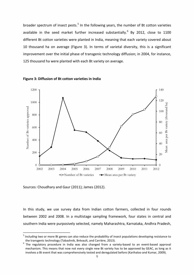
available in the seed market further increased substantially.6 By 2012, close to 1100
different Bt cotton varieties were planted in India, meaning that each variety covered about
10 thousand ha on average (Figure 3). In terms of varietal diversity, this is a significant
improvement over the initial phase of transgenic technology diffusion; in 2004, for instance,
125 thousand ha were planted with each Bt variety on average.
Figure 3: Diffusion of Bt cotton varieties in India
Sources: Choudhary and Gaur (2011); James (2012).
In this study, we use survey data from Indian cotton farmers, collected in four rounds
between 2002 and 2008. In a multistage sampling framework, four states in central and
southern India were purposively selected, namely Maharashtra, Karnataka, Andhra Pradesh,
5 Including two or more Bt genes can also reduce the probability of insect populations developing resistance to
the transgenic technology (Tabashnik, Brévault, and Carrière, 2013). 6 The regulatory procedure in India was also changed from a variety-based to an event-based approval
mechanism. This means that now not every single new Bt variety has to be approved by GEAC, as long as it involves a Bt event that was comprehensively tested and deregulated before (Karihaloo and Kumar, 2009).
0
20
40
60
80
100
120
140
0
200
400
600
800
1000
1200
2002 2003 2004 2005 2006 2007 2008 2009 2010 2011 2012M
ean
are
a pe
r Bt v
arie
ty (t
hous
and
ha)
Num
ber o
f Bt
var
ietie
s app
rove
d
Number of Bt varieties Mean area per Bt variety
10
and Tamil Nadu. In these states, we randomly selected 10 cotton-growing districts and 58
villages, using a combination of census data and agricultural production statistics. Within
each village, farm households were randomly chosen from complete lists of cotton
producers provided by the village heads. In total, 341 farmers were sampled in 2002. In
2004, a second round of the survey was carried out with the same farmers, whereby the
overall sample size was slightly increased. A third and a fourth round of data collection with
these farmers took place in 2006 and 2008, respectively. Further details of the survey are
provided by Kathage and Qaim (2012) and Krishna and Qaim (2012). In total, we have 1431
household observations over the four survey rounds; a few of these observations could not
be used for this analysis due to missing variables. The sample is representative for cotton
growers in central and southern India. The panel data provide an interesting empirical base
to analyze the effects of transgenic technology on on-farm varietal diversity and possible
dynamics with changes in the supply of transgenic varieties.
4. Empirical Framework
Testing hypothesis I
To test the first research hypothesis, we analyze impacts of transgenic technology on crop
yield and production risk. We expect that Bt technology increases yield (through reducing
insect pest damage) and reduces production risk (through reducing yield variability cause by
insect pests). Productivity-enhancing and risk-reducing effects are also expected through
maintaining on-farm varietal diversity. For the analysis, we use the framework proposed by
Just and Pope (1979) in a heteroscedastic regression model of the cotton production
function. The Just and Pope (1979) framework has been used previously to analyze effects of
Bt cotton (Crost and Shankar, 2008; Shankar, Bennett and Morse, 2008) and of varietal
diversity (Smale et al., 1998; Di Falco and Chavas, 2009), but not jointly in one study. Here,
we use cotton production per farm as dependent variable and regress this on a vector of
inputs and production factors. In addition, we include Bt technology adoption and varietal
diversity as explanatory variables. Bt adoption is represented as the area share of Bt cotton
in the total cotton area of the respective farm; this share ranges from 0 when Bt is not

11
adopted to 1 when the technology is adopted on the whole cotton area. Varietal diversity is
measured in terms of the number of cotton varieties cultivated on the farm in a given
season, regardless of whether these varieties are transgenic or conventional. The production
framework consists of a deterministic component to explain mean level of production, and a
risk function to explain production variance, as follows:
y𝑖𝑡 = 𝑓(𝑥𝑖𝑡𝑙,𝜎)�������𝑑𝑒𝑡𝑒𝑟𝑚𝑖𝑛𝑖𝑠𝑡𝑖𝑐
+ 𝑔(𝑥𝑖𝑡𝑚,𝜃)𝑢𝑖𝑡���������𝑟𝑖𝑠𝑘
… (1)
The deterministic component is elaborated in a generalized Cobb-Douglas function as,
E(y𝑖𝑡) = 𝑓(. ) = exp�𝜎0 + 𝜎1𝐷𝑖𝑡 + �𝜎𝑙1𝑥𝑖𝑡𝑙1
𝑙1
𝑙1=1
+ �𝜎𝑙2�̅�𝑖𝑙2
𝑙2
𝑙2=1
������������������������������
𝑙𝑖𝑛𝑒𝑎𝑟
�𝑥𝑖𝑡𝑙3𝜎𝑙3
𝑙3
𝑙3=1
� �̅�𝑖𝑙4𝜎𝑙4
𝑙4
𝑙4=1�����������𝑙𝑜𝑔𝑎𝑟𝑖𝑡ℎ𝑚𝑖𝑐
… (2)
and the risk function as,
V(y𝑖𝑡) = 𝑔2(. ) = 𝜃0 + � 𝜃𝑚1𝑥𝑖𝑡𝑚1
𝑚1
𝑚1=1
+ � 𝜃𝑚2�̅�𝑖𝑚2
𝑚2
𝑚2=1
+ 𝜈𝑖𝑡 + �̅�𝑖 … (3)
where y𝑖𝑡 is cotton production per farm in logarithmic form, 𝑥𝑖𝑡𝑙1 is the matrix of time-
variant explanatory variables in linear form (including share of Bt area and number of cotton
varieties), �̅�𝑖𝑙2 is the matrix of time-invariant explanatory variables in linear form, 𝑥𝑖𝑡𝑙3 is the
matrix of time-variant explanatory variables in logarithmic form, and �̅�𝑖𝑙4 is the matrix of
time-invariant explanatory variables in logarithmic form. Parameter vectors to be estimated
are 𝜎 and 𝜃, and 𝜈𝑖𝑡 and �̅�𝑖 are individual and time-specific stochastic disturbance terms. The
variance function 𝑔2(. ) is commonly specified as a linear function of production inputs,
human capital, and location-specific factors.
The production mean and variance functions are estimated using a three-step process, as
suggested by Just and Pope (1979). First, an ordinary least squares (OLS) regression on
production is estimated, accounting for heteroscedasticity. Second, the error terms are
derived from this model and used for estimation of the variance function 𝑔2(. ). Finally, a
generalized least squares (GLS) production model is estimated with the inverse of the
variance of predicted error terms from 𝑔2(. ) as analytical weights. The hypothesis that
12
transgenic technology increases yield and reduces production risk assumes that the
coefficient for Bt adoption has a positive sign in the GLS production model and a negative
sign in the variance model.
Random and fixed effects panel specifications are tested to address possible issues of
unobserved heterogeneity. The fixed effects model assumes that unobserved heterogeneity
is correlated with the regressors, while the random effects specification assumes that there
is no such correlation. If unobserved heterogeneity is correlated with any of the regressors
and also with the dependent variable, the random effects estimates will be biased. In our
case, Bt cotton adoption and on-farm varietal diversity are both possibly endogenous
regressors, so that a random effects model might suffer from systematic selection bias. A
Hausman specification test is performed to compare between the two specifications. When
there is a systematic difference, the fixed effects specification is preferred, as it controls for
the bias (Baltagi, 2005). However, when there is no systematic difference, the random
effects alternative is a more efficient estimator.
Testing hypotheses II and III
The second and third hypotheses are more specifically concerned with the impact of
transgenic technology on varietal diversity. Determinants of on-farm varietal diversity were
analyzed in a number of studies (e.g., Benin et. al., 2004; Nagarajan, Smale and Giewwe,
2007), but none of these studies addressed the impact of transgenic technology adoption.
We will start the analysis with some descriptive statistics, comparing levels of on-farm
varietal diversity between full Bt adopters, partial adopters, and non-adopters over the
survey years. Hypothesis II implies that on-farm diversity is lower among Bt adopters than
among non-adopters in the early years of diffusion, whereas hypothesis III would imply that
diversity increases in later years (especially in 2006 and 2008) with a larger number of Bt
varieties becoming available in the seed market.
However, comparison of descriptive statistics can only be a first indicator, because there
may be factors other than the increasing supply of Bt varieties that affect varietal diversity
over time. We control for such other factors in regression models, using measures of varietal
diversity as dependent and a set of possible determinants as independent variables. In a first
model (model 1), we express varietal diversity as explained above, namely in terms of the

13
total number of cotton varieties grown on a farm. Yet there are also more specific indices
that can be used to express varietal diversity, such as the Margalef index of varietal richness
or Simpson’s evenness index that both account for the size of the farm (Di Falco and
Perrings, 2003; Benin et al., 2004; Nagarajan, Smale, and Glewwe, 2007; Di Falco and Chavas,
2009).7 To test whether the way of measurement influences the results we use a second
model with the number of cotton varieties per ha of cotton (model 2) and a third model with
Simpson’s evenness index (model 3) as dependent variable. When only one single cotton
variety is grown on a farm, Simpson’s evenness index has a value of zero. Model 1 with a
count variable on the left-hand side is estimated with a Poisson specification, for model 2 we
use OLS, and model 3 with left-censoring of the dependent variable at zero is estimated with
a Tobit specification. Again, random and fixed effects models are estimated and compared
with a Hausman test.
In the set of explanatory variables, we include the farm area under cotton to control for
possible scale effects. As time-variant variable, we include Bt adoption in terms of the share
of the cotton area under this transgenic technology. Furthermore, we include a quadratic Bt
adoption term to test for possible non-linearity. The square term is of particular relevance,
because we expect that full adoption of transgenic technology will have a stronger effect on
diversity than partial adoption. Hypothesis II implies that the overall Bt effect is negative. To
test hypothesis III, we include the number of approved Bt varieties as an additional time-
variant explanatory variable. This is measured at the state level, because Bt varieties are
approved for specific states in India, depending on their suitability to local soil and climate
conditions (Karihaloo and Kumar, 2009; James, 2012). We expect that the number of Bt
varieties locally available in the seed market will affect the diversity on Bt adopting farms, so
we use an interaction term between the number of approved Bt varieties and Bt adoption.
Hypothesis III would imply that this interaction term has a positive and significant
coefficient. Other time-variant variables that represent the level of abiotic risk are irrigation
at the farm level and average rainfall measured at the district level over the last five cotton
growing seasons. We also include a number of time-invariant variables, such as household
7 The Margalef index of varietal richness is calculated as 𝑁−1
ln (𝐴), where N is the total number of varieties grown
on a farm of size A measured in square meters. Simpson’s evenness index is calculated as 1 − ∑ �𝐴𝑛𝐴�2
𝑛𝑛=1 ,
where 𝐴𝑛 is area under variety 𝑛.
14
characteristics (household size, age and education of household head) and state dummies,
which may also influence on-farm varietal diversity.
5. Results and Discussion
5.1. Impact of Bt adoption on cotton yield and production risk
In this section, we analyze the impact of Bt adoption on cotton yield and production risk with
descriptive statistics and a production function model, as outlined above. Table 1 shows
mean yield levels per ha of cotton for Bt adopters and non-adopters. These yield levels do
not refer to a specific plot on the farm, but are calculated as total cotton production on the
farm divided by cotton area. We differentiate between non-adopters of Bt, partial adopters,
and full adopters with 100% Bt adoption. The Table also differentiates between different
categories of varietal richness. Using the Margalef index, farms are divided into three
categories: (i) zero diversity (only one cotton variety per farm), (ii) low diversity (0 < richness
index ≤ 0.11), and (iii) high diversity (richness index > 0.11). We use 0.11 as the boundary
between low and high diversity, as this is the median of the Margalef index among the
sample farmers. The results in Table 1 show that mean cotton yield increases consistently
when the Bt area share increases. This holds true across all categories of varietal richness
and suggests that Bt technology is indeed yield increasing. The yield difference between full
adoption and non-adoption of Bt is 49% at zero varietal diversity, 62% when diversity is low,
and 55% when diversity is high. When looking at the overall sample (last column in Table 1),
a positive yield effect is also observed for increasing varietal diversity, although this is much
smaller than for Bt and not consistent with varying levels of Bt adoption.
To assess impacts on production risk with descriptive statistics, we use the coefficient of
variation (CoV) of yield as a normalized measure of dispersion. These values are also shown
in Table 1. As expected, Bt technology and varietal diversity both seem to be risk-reducing.
The CoV is 32% lower for full Bt adopters than for non-adopters, and it is 26% lower for
farms with high varietal diversity than for farms with zero diversity. This suggests that
adopting Bt may substitute for the insurance function of agrobiodiversity when only a small
number of Bt varieties is available in the seed market. However, production risk can be

15
further reduced when full Bt adopters maintain varietal diversity, which is possible only with
a larger number of Bt varieties available in the market.
Table 1. Mean yield and yield variability of Bt cotton adopters and non-adopters by
varietal diversity category
Bt adoption status
Varietal diversity
category Non-adoption
Partial
adoption Full adoption Overall
Zero diversity 1.29 1.78# 1.91 1.65***a
[0.68] [0.28] [0.48] [0.57]* a
Low diversity 1.31 1.47 2.14 1.72*** a
[0.59] [0.57] [0.39] [0.89]
High diversity 1.31 1.61 2.03 1.78*** a
[0.44] [0.47] [0.34] [0.42]
Overall 1.30 1.55**b 2.00**b 1.71***a, ***b
[0.62]**b [0.51] [0.42]***b [0.52]*a, ***b
Notes: N = 1417. Mean yield is measured in tons per hectare; coefficients of variation (CoV) are shown in square brackets. Varietal diversity categories are based on the Margalef index of varietal richness (see text). * , ** and *** imply that inter-group differences are statistically significant at the 0.10, 0.05 and 0.01 level, respectively. Mean yield differences are tested with the nonparametric k-sample mean comparison test; CoV differences are tested with Levene’s F test. a and b show whether the level of significance is calculated between different Bt adoption groups or between varietal diversity categories, respectively. # Partial adoption with zero diversity indicates that Bt and non-Bt versions of the same variety were adopted.
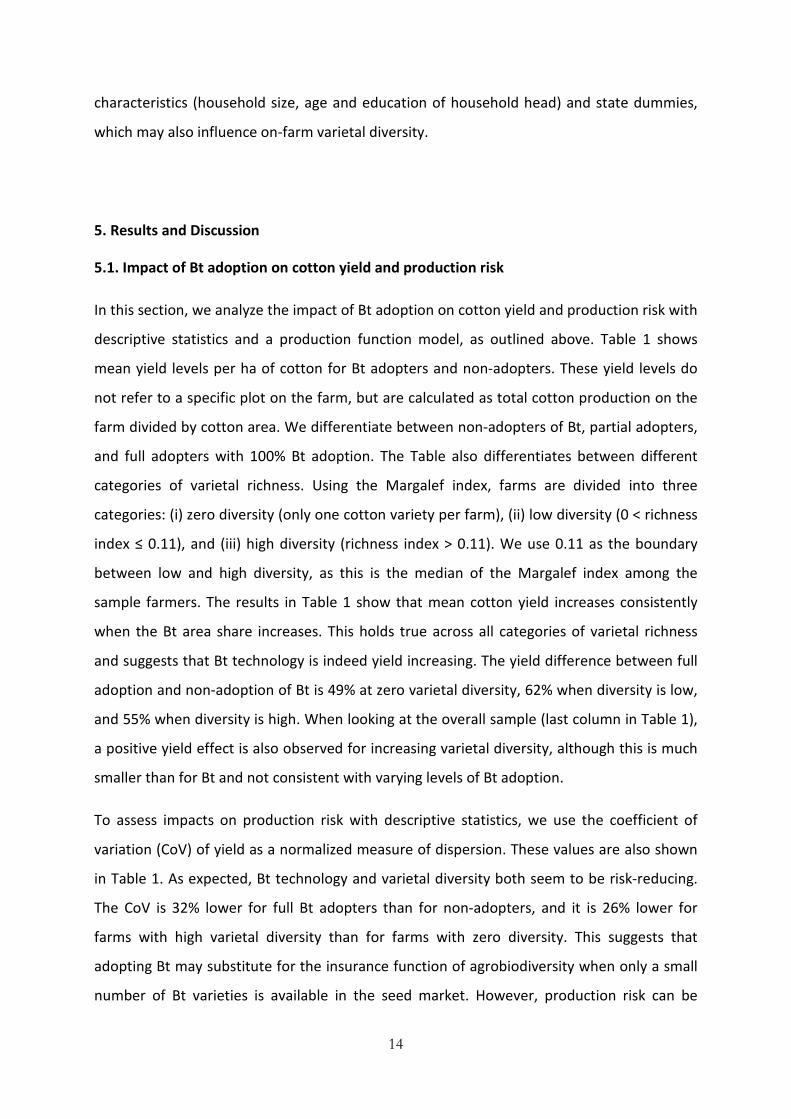
We now turn to the production function analysis, using the Just and Pope (1979) framework.
Summary statistics of the explanatory variables are shown in Table A1 in the Appendix.8 For
both the mean production and production variance functions, the Hausman test suggests
that the fixed and random effects estimates are systematically different at a 0.01 level of
significance. Hence, fixed effects specifications are preferred. Estimation results are shown
in Table 2. Bt adoption has a positive and significant coefficient on mean production levels. 8 In Table A1, we divide the observations into an early Bt diffusion phase (phase I, comprising 2002 and 2004)
and a later diffusion phase (phase II, comprising 2006 and 2008). This distinction is of interest, because Bt adoption increased over time, and also the number of Bt varieties available in the market increased significantly in the later phase.

16
Controlling for other factors and estimating at the sample mean of varietal diversity, Bt
adoption increased cotton yield by 28% in 2002. The interaction terms between Bt adoption
and the year dummies have insignificant coefficients, indicating that the Bt yield effect
remained stable over time. The year dummies themselves have positive and significant
coefficients in the mean production function, implying that cotton yields increased over time
also among the non-adopters of Bt technology. This may be due to general progress in
breeding and agronomy. In addition, widespread adoption of Bt may have contributed to
area-wide suppression of pest populations (Krishna and Qaim, 2012). Such positive spillovers
of widespread Bt cotton adoption were also observed in China (Wu et al., 2008).
The number of cotton varieties grown has a positive impact on mean production levels, too,
confirming the productivity-enhancing function of varietal diversity. This effect has also been
shown in other contexts by Di Falco and Chavas (2009), Di Falco, Bezabih and Yesuf (2010),
and Bangwayo-Skeete, Bezabih, and Zikhali (2012), among others. One additional variety
grown on the farm increases cotton yield by about 5%. The interaction between Bt adoption
and varietal diversity is insignificant, indicating that Bt adoption does not affect the
productivity-enhancing function of varietal diversity. However, when we compare effect
sizes, the yield impact of varietal diversity is lower than that of Bt adoption. For instance, an
average farmer with five conventional cotton varieties could switch to one single Bt variety,
without suffering a decline in yield. This suggests that – from a mere mean yield perspective
– there may be incentives to reduce on-farm varietal diversity when only a small number of
Bt varieties is available in the market.9
Crop duration, irrigation, rainfall, and off-farm income of households are also found to have
positive impact on mean cotton production (Table 2). The magnitude of the cotton area
coefficient indicates a negative scale effect: a 1% increase in area is associated with only a
0.84% increase in production. Together with the positive coefficient of varietal diversity, this
result suggests that the functioning of the system is positively affected by the degree of
fragmentation.
9 Kathage and Qaim (2012) showed that Bt adoption does not only increase mean yield, but also mean profit
for cotton farmers in India.
17
Table 2. Cotton production and risk function estimates
Cobb-Douglas mean production function (fixed effects GLS)
Production variance function
(fixed effects) Bt adoption [0-1 area share] 0.332***
(0.110) -0.413a (0.349)
Bt adoption * Year 2004 [interaction] -0.113 (0.129)
0.482 (0.407)
Bt adoption * Year 2006 [interaction] -0.072 (0.146)
0.444 (0.463)
Bt adoption * Year 2008 [interaction] -0.245 (0.357)
0.253 (1.102)
Number of cotton varieties grown 0.049* (0.026)
0.078 (0.075)
Bt adoption * Number of cotton varieties grown [interaction]
-0.030 (0.029)
-0.172**a (0.086)
Date of sowing [number of days from May 1st]# 0.029 (0.053)
0.189 (0.179)
Duration of crop [number of days]# 0.659*** (0.126)
-0.113 (0.396)
Cotton area [ha]# 0.839*** (0.039)
4.E-06 (0.118)
Chemical fertilizer [tons/ha]# 0.049 (0.031)
-0.067 (0.095)
Pesticide application [dummy] 0.027 (0.076)
0.617** (0.268)
Quantity of pesticide [kg/ha] ## 0.006 (0.018)
-0.009 (0.058)
Other input application [dummy] -0.011** (0.043)
-0.114 (0.136)
Value of other inputs [thousand rupees/ha] ## -0.055 (0.026)
0.067 (0.084)
Weeding operations [number] 0.019 (0.016)
-0.032 (0.050)
Irrigation applications [number] 0.023*** (0.007)
0.012 (0.021)
Rainfall at district level [millimeters]# 0.152*** (0.054)
-0.166 (0.167)
Household size [number] 4.E-05 (0.007)
0.026 (0.021)
Off-farm income [thousand rupees/year] 0.001*** (0.000)
-3.E-04 (0.001)
Year 2004 [dummy] 0.379*** (0.061)
-0.362** (0.170)
Year 2006 [dummy] 0.606*** (0.108)
-0.381 (0.331)
Year 2008 [dummy] 0.656* (0.346)
-0.031 (1.061)
Model intercept -4.915*** (0.848)
-2.851 (2.691)
Adjusted R2 0.80*** 0.45*** Hausman test statistic 83.51*** 226.03***
Notes: N = 1417. Coefficients are shown with robust standard errors in parentheses. # Variables included in logarithmic form; ## Logarithms are taken for strictly positive values; 0 otherwise. *, **, *** Statistically significant at the 0.1, 0.05 and 0.01 level, respectively. a Joint significance at 0.05 level.

18
In the production variance function, which is shown in the second column of Table 2, most of
the variables are statistically insignificant. One exception is the interaction term between Bt
adoption and varietal diversity, which has a negative and significant coefficient, suggesting
that these two factors have synergistic effects. Moreover, Bt adoption and this interaction
term are jointly significant: a one percentage point increase in Bt area reduced yield risk by
0.71% in 2002. Somewhat surprisingly, the varietal diversity variable itself is insignificant in
this model. In this context, the insurance function of varietal diversity seems to be weaker
than that of Bt adoption, as the descriptive statistics had already suggested. In summary, this
analysis shows that transgenic technology adoption increases yield and reduces production
risk, thus confirming our first research hypothesis.
5.2. Impact of Bt adoption on varietal diversity
With Bt technology increasing mean yield and reducing production risk, farmers may have an
incentive to reduce on-farm varietal diversity when only a small number of Bt varieties is
available. In other words, transgenic technology may contribute to agrobiodiversity erosion
in such situations. We now investigate whether such erosion actually took place for the case
of Bt cotton in India. We start by comparing different diversity indicators between the early
Bt diffusion phase with a low number of approved Bt varieties (phase I, comprising 2002 and
2004) and the later diffusion phase with a much larger number of approved Bt varieties
(phase II comprising 2006 and 2008). Bt technology adoption, measured as the share of Bt
cotton in the total cotton area, had increased from 25% in phase I to 92% in phase II. The
comparisons are summarized in Table 3 (further details are given in Table A2 in the
Appendix). Looking at the sample as a whole on the left-hand side of Table 3, we find no
significant difference between the two phases in any of the diversity measures. In phase I,
many farmers adopted Bt only partially, so that the diversity status was maintained through
growing conventional cotton varieties on the same farm. In phase II, the availability of more
Bt varieties helped farmers to preserve diversity even with full Bt adoption.

19
Table 3: On-farm varietal diversity with and without Bt cotton
Overall
Bt adoption status
Phase I
[2002 & 2004]
Phase II
[2006 & 2008]
Non-adopters in phase
I Full-adopters in phase II
Number of cotton varieties grown 2.03
(0.05)
2.11
(0.05)
1.77
(0.06)
2.17***
(0.05)
Cotton area [ha]
2.13
(0.08)
2.30
(0.08)
1.85
(0.09)
2.32***
(0.09)
Number of cotton varieties per ha
(weighted by area)
0.94
(0.02)
0.92
(0.02)
0.96
(0.03)
0.93
(0.02)
Margalef’s varietal richness index 0.10
(<0.01)
0.11
(<0.01)
0.08
(0.01)
0.11***
(0.01)
Simpson’s evenness index 0.31
(0.01)
0.33
(0.01)
0.25
(0.01)
0.34***
(0.01)
Number of observations 703 722 405 646
Note: Mean values are shown with standard errors in parenthesis. *** Difference between full adopters in phase II and non-adopters in phase I is statistically significant at the 0.01 level. No significant differences are observed between phase I and II for the overall sample.

20
The right-hand part of Table 3 looks at the diversity impacts of Bt technology more
specifically, by comparing non-adopters of Bt in phase I with full adopters in phase II.
Strikingly, varietal diversity was significantly higher for the full adopters in phase II,
suggesting that the adoption of Bt technology did not lead to diversity erosion. Yet this
comparison masks some interesting variation that occurred within each of the phases. Table
A2 shows that full adoption of Bt in phase I was associated with lower varietal diversity. On
the other hand, non-adoption of Bt was associated with lower diversity in phase II.
To analyze these effects further, we estimate different varietal diversity regression models,
as explained above. Estimation results are shown in Table 4. In model 1, the Hausman test
indicates no significant difference between the random and fixed effects results, so the
random effect specification is preferred. In model 2, a significant difference is detected, so
we use the fixed effects specification. For the Tobit model (model 3), we use the random
effects specification. The results of all three models are similar. In all cases, Bt adoption as
such has a positive and significant coefficient, which may be surprising at the first glance.
However, this effect is primarily driven by partial adoption. With full adoption (Bt area share
of 1), Bt decreases varietal diversity because the negative square term overcompensates the
positive direct effect. This negative impact of Bt technology on varietal diversity holds when
the supply of different Bt varieties is small, thus confirming hypothesis II. With more Bt
varieties supplied, the loss of on-farm diversity is reduced, as can be seen from the positive
and significant interaction term between Bt adoption and the number of approved Bt
varieties.

21
Table 4: Determinants of on-farm varietal diversity
Model 1: Number of varieties per farm (Poisson,
random effects)
Model 2: Number of varieties per ha (linear, fixed
effects)
Model 3: Simpson’s evenness index (Tobit, random
effects) Bt adoption [0-1 area share] 1.461***
(0.238) 1.152***
(0.289) 1.017***
(0.084) Square of Bt adoption -1.709***
(0.255) -1.250*** (0.295)
-1.112*** (0.086)
Number of approved Bt varieties at state level
-0.034** (0.017)
-0.021 (0.016)
-0.019*** (0.005)
Bt adoption * Number of approved Bt varieties at state level [interaction]
0.012*** (0.004)
0.006** (0.003)
0.004*** (0.001)
Cotton area [ha] 0.085*** (0.007)
-0.167*** (0.016)
0.042*** (0.003)
Irrigation facility [dummy] 0.051*** (0.040)
0.064 (0.054)
0.024* (0.013)
Mean rainfall during last five years [millimeters]
0.055 (0.078)
-0.103 (0.099)
0.034 (0.023)
Age of household head [years] -0.003** (0.002)
-0.002 (0.001)
Education of household head [years] 0.002 (0.004)
2.E-04 (1.E-03)
Household size [number] -0.003 (0.005)
-2.E-04 (0.009)
-0.001 (0.002)
Off-farm income [thousand rupees/year]
-2.E-04 (2.E-04)
-3.E-04 (3.E-04)
-1.E-04* (7.E-05)
Andhra Pradesh [dummy] -0.249*** (0.053)
-0.075*** (0.020)
Karnataka [dummy] -0.570*** (0.054)
-0.246*** (0.019)
Tamil Nadu [dummy] -0.553*** (0.118)
-0.245*** (0.035)
Year 2004 [dummy] 0.248*** (0.059)
0.049 (0.056)
0.106 (0.018)
Year 2006 [dummy] 1.041** (0.494)
0.464 (0.483)
0.591*** (0.160)
Year 2008 [dummy] 3.726 (2.378)
2.224 (2.359)
2.386*** (0.784)
Model intercept 0.440 (0.521)
2.410*** (0.681)
0.143 (0.154)
Adjusted R2 0.64*** Log-likelihood -2056.06 82.87 Wald χ2 522.55*** 826.78*** Hausman test statistic 11.29 29.92*** NA Notes: N = 1425. Coefficients are shown with robust standard errors in parentheses. . *, **, *** Statistically significant at the 0.1, 0.05 and 0.01 level, respectively.

22
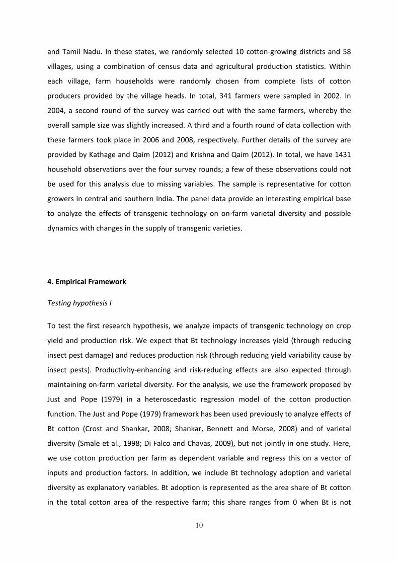
To analyze the relationship between Bt adoption, supply of Bt varieties, and on-farm varietal
diversity further, we use the model estimates for some predictions, as shown in Figure 4.
These predictions are based on model 2, where the dependent variable is the number of
cotton varieties grown on a farm normalized by cotton area. The two curves shown
represent the situation in technology diffusion phases I and II. In phase I, with only limited
supply of transgenic varieties, full adoption of Bt had a negative impact on varietal diversity
if compared to zero Bt adoption. However, partial Bt adopters were keeping higher levels of
varietal diversity compared to both full adopters and zero adopters. In other words, in that
early phase farmers had to relinquish diversity to accomplish higher level of Bt adoption. In
phase II, the impact was different. The development and approval of many additional Bt
varieties allowed Bt adopters to restore varietal diversity. The predictions suggest that on-
farm varietal diversity in phase II with full Bt adoption was in the same magnitude as with
zero Bt adoption in phase I. These results confirm research hypothesis III.
Figure 4: Impact of Bt adoption on-farm varietal diversity
Note: Predictions are based on model 2 of Table 4.
0.8
1.0
1.2
1.4
1.6
0.0 0.2 0.4 0.6 0.8 1.0
Nnu
mbe
r of v
arie
ties p
er h
ecta
re
Bt adoption [area share]
Phase I [2002 & 2004] Phase II [2006 & 2008]

23
Another noteworthy result of this analysis is the negative direct effect of the number of
approved Bt varieties on varietal diversity, which is significant in two of the models in Table
4. This implies that a larger supply of Bt varieties leads to lower on-farm varietal diversity
among non-adopters of Bt. Indeed, Figure 4 shows a low level of diversity with zero Bt
adoption in phase II. With over 90% adoption of Bt, seed companies now focus primarily on
supplying transgenic seeds; it is not lucrative anymore to also supply non-Bt versions of all
varieties. Given the high adoption of Bt, this is of little relevance for aggregate varietal
diversity, but it may certainly affect varietal choices of individual farmers who prefer not to
adopt Bt technology.
6. Conclusion and Policy Implications
During the Green Revolution it was observed that many local crop varieties were replaced
with a few high-yielding ones in large parts of the developing world. There are widespread
concerns that such agrobiodiversity erosion may continue and be accelerated through
transgenic crop technologies. However, transgenic crops differ from high-yielding varieties of
the Green Revolution and so warrant a closer look. In this study, we have analyzed the
impact of transgenic crops on varietal diversity, first conceptually and then using the
concrete example of Bt cotton in India.
From the private perspective of farmers, varietal diversity can have productivity-enhancing
and risk-reducing effects. We have hypothesized that transgenic crops can also increase
productivity and reduce production risk and may therefore substitute for on-farm varietal
diversity. Yet, a transgenic technology is not only one new variety; the same genes coding for
desirable traits can be introgressed into many varieties that are well adapted to various soil
and climate conditions. If many transgenic varieties with the same traits are developed and
adopted, agrobiodiversity can be preserved.
These hypotheses were confirmed in the empirical analysis. Insect-resistant Bt cotton has
significantly increased productivity and reduced production risk for smallholder farmers in
India. The panel data also allowed us to study developments over time. The observed
dynamics are very interesting because seed market conditions changed considerably,

24
providing a quasi-experimental setting to analyze the diversity consequences of differing
numbers of Bt cotton varieties. In the early phase of Bt technology diffusion, the Indian
regulatory authorities had only approved a very small number of Bt varieties, while in later
years many more Bt varieties became available in the seed market. Indeed, farmers that fully
adopted Bt cotton in the early years, reduced their varietal diversity. In later years, with
more Bt varieties available, these same technology adopters restored varietal diversity.
These results underline that a combination of transgenic technology and high levels of
varietal diversity is possible, and is even further increasing productivity and reducing
production risk.
Overall, cotton varietal diversity in India with a Bt adoption rate of over 90% is now at the
same level or even higher than it was before the introduction of this transgenic technology.
Interestingly, even in the early phase of technology diffusion, with only a few Bt varieties
available in the market, average diversity did not decline significantly, because many farmers
adopted Bt only partially and maintained varietal diversity through growing conventional
varieties on the same farm. This may be related to a general farmer preference for on-farm
varietal diversity. Yet we have shown that full adoption would have been economically
advantageous for many even with only a few Bt varieties available. Hence, we suppose that
the observed partial adoption in the early phase was also a reflection of typical smallholder
cautiousness. Smallholder farmers often adopt new technologies partially in the beginning,
and increase adoption intensity when they are more certain that the technology is really
beneficial for them. This implies that cotton varietal diversity would likely have been
reduced if more Bt varieties had not become available in later years.
The empirical results from India do not necessarily hold for other situations, but one general
conclusion can be drawn nevertheless: transgenic technology can help to preserve crop
varietal diversity, but the concrete outcome depends on various institutional factors that
determine how many transgenic varieties are available in the market. We now discuss a few
of these institutional factors and also derive some policy implications. First, the biosafety
regulatory framework matters. In India, the regulatory authorities were slow in the
beginning to approve additional transgenic varieties, mainly due to the public debate about
possible risks associated with transgenic technology. However, once a transgenic event has
been tested and deregulated, introgressing that same event into other varieties cannot

25
reasonably be expected to lead to new risks (Bradford et al., 2005). Hence, a complex
regulatory process for each new transgenic variety jeopardizes agrobiodiversity without
increasing safety levels. Second, local breeding capacities in a country play an important
role. India has a strong public and private breeding sector for cotton. Hence, many
companies were technically able to introgress a transgenic trait into their varieties and
breeding lines. Such introgression of an available transgenic trait is less complicated than
identifying the trait and developing the transformation event, but it still requires some
capacity that may not be available in many poorer countries in Africa. Public support through
development organizations or international agricultural research centers may be required to
ensure that transgenic traits of interest are introgressed into multiple local varieties.
Innovative models of public-private partnership may also be an interesting approach in some
situations (Krishna and Qaim, 2007). Third, IPRs may play an important role. Many of the
transgenic technologies available so far are not patented in developing countries, so that
local organizations can use these technologies for free or with relatively simple licensing
agreements for introgression into their own varieties and breeding lines. Stronger IPRs may
involve more complex licensing agreements. If many local organizations can obtain a license
from the IPR holder, agrobiodiversity could be preserved. Restricted licenses to only one or a
few organizations, however, could contribute to agrobiodiversity erosion. Such institutional
aspects should be considered when designing national policies and regulatory frameworks
for transgenic technologies.
26
References
Baltagi, B.H. 2005. Econometric Analysis of Panel Data (4th edition). West Sussex: John Wiley
& Sons.
Bangwayo-Skeete, P.F., Bezabih, M., and Zikhali, P. 2012. Crop biodiversity, productivity and
production risk: panel data micro-evidence from Ethiopia. Natural Resources Forum, 36:
263-273.
Baumgärtner, S. and Quaas, M. F. 2010. Managing increasing environmental risks through
agrobiodiversity and agrienvironmental policies. Agricultural Economics, 41(5): 483-496.
Bellon, M.R., and Berthaud, J. 2004. Transgenic maize and the evolution of landrace diversity
in Mexico. The importance of farmers’ behavior. Plant Physiology, 134: 883-888.
Benin, S., Smale, M., Pender, J. Gebremedhin, B. and Ehui, S. 2004. The economic
determinants of cereal crop diversity on farms in the Ethiopian highlands. Agricultural
Economics, 31: 197-208.
Birthal, P.S., Sharma, O.P., Kumar, S., and Dhandapani, A. 2000. Pesticide use in rainfed
cotton: frequency, intensity and determinants. Agricultural Economics Research Review,
13(2): 107-122.
Boreux, V., Kushalappa, C.G., Vaast, P., Ghazoul, J., 2013. Interactive effects among
ecosystem services and management practices on crop production: pollination in coffee
agroforestry systems. Proceedings of the National Academy of Sciences USA, 110: 8387-
8392.
Bradford, K. J., Van Deynze, A., Gutterson, N., Parrott, W., and Strauss, S. H. 2005. Regulating
transgenic crops sensibly: lessons from plant breeding, biotechnology and
genomics. Nature Biotechnology, 23(4), 439-444.
Brush, S.B. 2000. “The issues of in situ conservation of crop genetic resources.” In Brush
(ed.), Genes in the Field: On-Farm Conservation of Crop Diversity. IDRC/IPGRI/Lewis
Publishers.
Carpenter, J. E. 2010. Peer-reviewed surveys indicate positive impact of commercialized GM
crops. Nature Biotechnology, 28:319–321.
Chavas, J-P., and Di Falco, S., 2012. On the productive value of crop biodiversity: evidence
from the highlands of Ethiopia. Land Economics, 88(1): 58-74.
Choudhary, B., and Gaur, K. 2010. Bt Cotton in India: A Country Profile. International Service
for the Acquisition of Agri-biotech Applications (ISAAA), Ithaca, New York: ISAAA.

27
Cooper, D., Engels, J. and Frison, E.A.. 1994. A Multilateral System for Plant Genetic
Resources: Imperatives, Achievements and Challenges. Issues in Genetic Resources No.
2. Bioversity International, Rome.
Crost, B., Shankar, B., Bennett, R. and Morse, S. 2007. Bias from farmer self-selection in
genetically modified crop productivity estimates: evidence from Indian data. Journal of
Agricultural Economics, 58(1): 24-36.
Crost, B., and Shankar, B. 2008. Bt-cotton and production risk: panel data estimates.
International Journal of Biotechnology, 10(2/3): 123-31.
Di Falco, S., and Perrings, C. 2003. Crop genetic diversity, productivity and stability of
agroecosystems. A theoretical and empirical investigation. Scottish Journal of Political
Economy, 50(2), 207–217.
Di Falco, S., and Chavas, J-P. 2009. On crop biodiversity, risk exposure and food security in
the Highlands of Ethiopia. American Journal of Agricultural Economics, 91(3): 599-611.
Di Falco, S., Bezabih, M., and Yesuf, M. 2010. Seeds for livelihood: crop biodiversity and food
production in Ethiopia. Ecological Economics, 69(8), 1695-1702.
Harlan, J.R. 1975. Our vanishing genetic resources. Science, 188: 618–621.
Holt-Gimenez, E., Altieri, M.A. 2013. Agroecology, food sovereignty, and the new green
revolution. Agroecology and Sustainable Food Systems, 37: 90-102.
Huang, J., Mi, J.W., Lin, H., Wang, Z.J., Chen, R.J., Hu, R.F., Rozelle, S., Pray, C. 2010. A decade
of Bt cotton in Chinese fields: assessing the direct effects and indirect externalities of Bt
cotton adoption in China. Science China Life Sciences, 53: 981-991.
James, C. 2012. Global Status of Commercialized Biotech/GM Crops: 2012. International
Service for the Acquisition of Agri-biotech Applications Brief No. 44. Ithaca, New York:
ISAAA.
Just, R. E., and Pope, R.D. 1979. Production function estimation and related risk
considerations. American Journal of Agricultural Economics, 61: 276-84.
Karihaloo, J.L., and Kumar, P.A. 2009. Bt Cotton in India: A Status Report (Second Edition).
New Delhi: Asia-Pacific Consortium on Agricultural Biotechnology (APCoAB).
Kathage, J., and Qaim, M. 2012. Economic impacts and impact dynamics of Bt (Bacillus
thuringiensis) cotton in India. Proceedings of the National Academy of Sciences USA,
109(29): 11652–11656.
28
Kolady, D.E., and Lesser, W. 2012. Genetically-engineered crops and their effects on varietal
diversity: a case of Bt eggplant in India. Agriculture and Human Values, 29: 3-15.
Krishna, V.V., Byju, N. G., and Tamizheniyan, S. 2003. Integrated pest management in Indian
agriculture. IPM World Textbook, ed. EB Radcliff, Hutchson, WD St. Paul, MN.
Krishna, V.V., and Qaim, M. 2007. Estimating the adoption of Bt eggplant in India: who
benefits from public-private partnership? Food Policy 32(5/6): 523-543.
Krishna, V.V., and Qaim, M. 2012. Bt cotton and sustainability of pesticide reductions in
India. Agricultural Systems, 107: 47-55.
Krishna, V.V., Drucker, A.G., Pascual, U., Raghu, P.T. and Israel Oliver King, E.D. 2013.
Estimating compensation payments for on-farm conservation of agricultural biodiversity
in developing countries. Ecological Economics 87:110-123.
Millennium Ecosystem Assessment 2005. Ecosystems and Human Well-Being: A Framework
for Assessment; Washington, DC. Island Press.
Nagarajan, L., Smale, M., and Glewwe, P. 2007. Determinants of millet diversity at the
household-farm and village-community levels in the drylands of India: the role of local
seed systems. Agricultural Economics, 36: 157-167.
Qaim, M., and Zilberman, D., 2003. Yield effects of genetically modified crops in developing
countries. Science, 299(5608): 900-902.
Qaim, M., Subramanian, A., Naik, G., and Zilberman, D. 2006. Adoption of Bt cotton and
impact variability: Insights from India. Review of Agricultural Economics, 28(1), 48-58.
Qaim, M. 2009. The economics of genetically modified crops. Annual Review of Resource
Economics, 1: 665–694.
Qaim, M., Yarkin, C., and Zilberman, D. 2005. Impact of biotechnology on crop genetic
diversity. In Cooper, J., Lipper, L.M., and Zilberman, D. (ed.) Agricultural Biodiversity and
Biotechnology in Economic Development, Springer Science and Business Media, Inc., pp.
283-308.
Qaim, M., and Kouser, S. 2013. Genetically modified crops and food security. PLOS ONE, 8(6),
e64879.
Raven, P.H. 2010. Does the use of transgenic plants diminish or promote biodiversity? New
Biotechnology, 27: 528-533.

29
Rosenzweig, C., Iglesias, A., Yang, X. B., Epstein, P. R., and Chivian, E., 2001. Climate change
and extreme weather events; implications for food production, plant diseases, and
pests. Global Change & Human Health, 2(2): 90-104.
Shankar, B., Bennett, R., and Morse, S. 2008. Production risk, pesticide use and GM crop
technology in South Africa. Applied Economics, 40: 2489-2500.
Shiva, V., 1991. The Green Revolution in the Punjab. The Ecologist 21: 57-60.
Smale, M., Just, R. E., and Leathers, H. D. 1994. Land allocation in HYV adoption models: an
investigation of alternative explanations. American Journal of Agricultural
Economics, 76(3), 535-546.
Smale, M. 1997. The Green Revolution and wheat genetic diversity: some unfounded
assumptions. World Development, 25(8): 1257-1269.
Smale, M., Hartell, J., Heisey, P.W., and Senauer, B. 1998. The contribution of genetic
resources and diversity to wheat production in the Punjab of Pakistan. American Journal
of Agricultural Economics, 80: 482-93.
Smale, M., 2006. Concepts, metrics and plan of the book. In Smale, M. (ed.), Valuing crop
biodiversity: On-farm genetic resources and economic change. Oxfordshire: CAB
International, pp. 1-17.
Smale, M., Zambrano, P., Gruére, G., Falck-Zepeda, J., Matuschke, I., Horna, D., Nagarajan, L.,
Yerramareddy, I., and Jones, H. 2009. Measuring the economic impacts of transgenic
crops in developing agriculture during the first decade: approaches, findings, and future
directions. International Food Policy Research Institute Review No. 10. Washington DC.:
IFPRI.
Subramanian, A., and Qaim, M. 2010. The impact of Bt cotton on poor households in rural
India. Journal of Development Studies, 46(2), 295-311.
Tabashnik, B.E., Brévault, T., and Carrière, Y. 2013. Insect resistance to Bt crops: lessons from
the first billion acres. Nature Biotechnology, 31(6): 510-521.
Tripp, R. 1996. Biodiversity and modern crop varieties: sharpening the debate. Agriculture
and Human Values 13(4), 48-63.
Tripp, R. 2009. Transgenic cotton and institutional performance. In Tripp (ed.), Biotechnology
and Agricultural Development: Transgenic Cotton, Rural Institutions and Resource-Poor
Farmers, New York: Routledge., pp. 88-104.

30
Van Dusen, M. E., and Taylor, J.E. 2005. Missing markets and crop diversity: evidence from
Mexico. Environment and Development Economics, 10(4): 513–531.
Van Straalen, N. M., and Timmermans, M. J. 2002. Genetic variation in toxicant-stressed
populations: an evaluation of the “genetic erosion” hypothesis. Human and Ecological
Risk Assessment, 8(5), 983-1002.
Wu, K.M., Lu, Y.-H., Feng, H.-Q., Jiang, Y.-Y., and Zhao, J.-Z. 2008. Suppression of cotton
bollworm in multiple crops in China in areas with Bt toxin-containing cotton. Science
321, 1676–1678.
Zilberman, D., Ameden, H., and Qaim, M. 2007. The impact of agricultural biotechnology on
yields, risks, and biodiversity in low-income countries. Journal of Development
Studies, 43(1), 63-78.

31
Appendix
Table A1: Summary statistics of explanatory variables used in regression models
Unit of measurement
Phase I [2002 & 2004] Phase II [2006 & 2008] Mean (Std. dev.) Mean (Std. dev.)
Variables used in production function analysis [N = 1417]
Bt adoption, area share relative to total cotton area 0-1 0.25 (0.01) 0.92*** (0.01) Date of sowing number of days from
May 1st 56.76 (0.75) 55.10* (0.66)
Duration of the crop number of days 218.27 (1.16) 218.92 (1.42) Cotton area ha 2.13 (0.08) 2.30 (0.08) Chemical fertilizer tons/ha 0.59 (0.01) 0.61 (0.01) Pesticide application dummy 0.96 0.93*** Quantity of pesticides, if applied kg/ha 8.26 (0.27) 2.82*** (0.12) Other input application (other than fertilizer, pesticide, and labor)
dummy 0.21 0.36***
Value of other inputs, if applied thousand rupees/ha 1.21 (0.43) 1.14 (0.16) Weeding operations number 3.07 (0.05) 2.86* (0.05) Irrigation applications number 2.26 (0.15) 2.18 (0.11) Rainfall at district level (current cotton season) millimeters 648.60 (10.23) 724.14*** (9.30) Household size number of members 6.45 (0.13) 6.29 (0.15) Off-farm income thousand rupees/year 28.37 (4.19) 27.79 (2.55)
Variables used in varietal diversity analysis [N = 1425] Approved Bt varieties at state level number 3.51 (0.02) 93.69*** (2.16) Irrigation facility dummy 0.50 0.58*** Mean rainfall during last five years millimeters 914.75 (16.66) 747.08*** (5.71) Age of household head years 44.60 (0.47) 45.40 (0.47) Education of household head years of schooling 7.34 (0.19) 7.14 (0.19) Andhra Pradesh dummy 0.30 0.32 Karnataka dummy 0.30 0.30 Tamil Nadu dummy 0.09 0.04***
*, *** Difference between phase I and II is statistically significant at the 0.1 and 0.01 level, respectively.
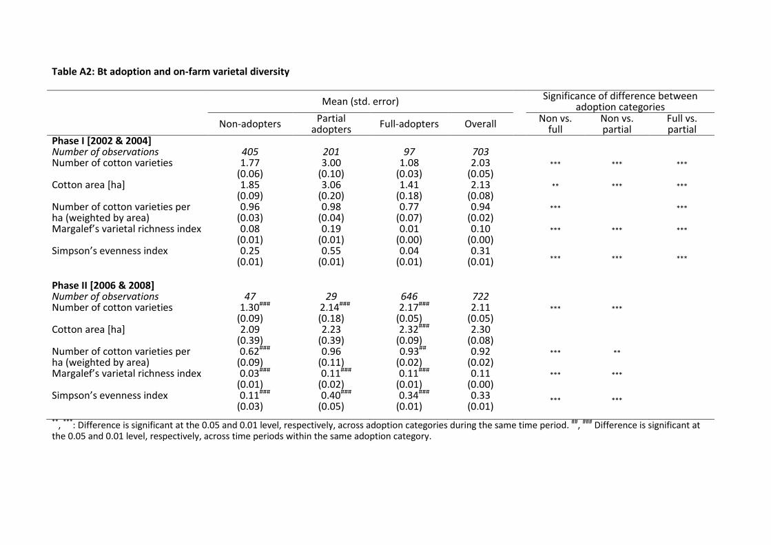
Table A2: Bt adoption and on-farm varietal diversity
Mean (std. error) Significance of difference between adoption categories
Non-adopters Partial adopters Full-adopters Overall Non vs.
full Non vs. partial
Full vs. partial
Phase I [2002 & 2004]
Number of observations 405 201 97 703
Number of cotton varieties 1.77 (0.06)
3.00 (0.10)
1.08 (0.03)
2.03 (0.05)
*** *** ***
Cotton area [ha]
1.85 (0.09)
3.06 (0.20)
1.41 (0.18)
2.13 (0.08)
** *** ***
Number of cotton varieties per ha (weighted by area)
0.96 (0.03)
0.98 (0.04)
0.77 (0.07)
0.94 (0.02)
*** ***
Margalef’s varietal richness index 0.08 (0.01)
0.19 (0.01)
0.01 (0.00)
0.10 (0.00)
*** *** ***
Simpson’s evenness index 0.25 (0.01)
0.55 (0.01)
0.04 (0.01)
0.31 (0.01)
*** *** ***
Phase II [2006 & 2008]
Number of observations 47 29 646 722 Number of cotton varieties 1.30###
(0.09) 2.14###
(0.18) 2.17###
(0.05) 2.11
(0.05) *** ***
Cotton area [ha]
2.09 (0.39)
2.23 (0.39)
2.32### (0.09)
2.30 (0.08)
Number of cotton varieties per ha (weighted by area)
0.62### (0.09)
0.96 (0.11)
0.93##
(0.02) 0.92
(0.02) *** **
Margalef’s varietal richness index 0.03### (0.01)
0.11### (0.02)
0.11### (0.01)
0.11 (0.00)
*** ***
Simpson’s evenness index 0.11### (0.03)
0.40### (0.05)
0.34### (0.01)
0.33 (0.01)
*** ***
**, ***: Difference is significant at the 0.05 and 0.01 level, respectively, across adoption categories during the same time period. ##, ### Difference is significant at the 0.05 and 0.01 level, respectively, across time periods within the same adoption category.