zero discharge fluid dynamic gauging for studying the
TRANSCRIPT

Zero discharge fluid dynamic gauging for studying the swelling of
soft solid layers
Shiyao Wang and D. Ian Wilson*
Revised Manuscript
IE 2015 019564
Ind. Eng. Chem. Res. Des.
July 2015
Department of Chemical Engineering & Biotechnology
New Museums Site
Pembroke Street
Cambridge
CB2 3RA
UK
*Corresponding author
Dr Ian Wilson
Tel +44 1223 334791
FAX +44 1223 334796
E-mail [email protected]
1
Zero discharge fluid dynamic gauging for studying the swelling of soft solid
layers
Shiyao Wang and D. Ian Wilson
Department of Chemical Engineering and Biotechnology, New Museums Site, Pembroke
Street, Cambridge, CB2 3RA, UK
Abstract
A bench-top device fluid dynamic gauging device to study the swelling or shrinking of soft
solid layers immersed in a liquid environment in situ and in real time is demonstrated. A
particular feature is that the volume of liquid is isolated, hence the name Zero net discharge
Fluid Dynamic Gauging (ZFDG), which renders ZFDG suitable for aseptic operation. For the
1.78 mm nozzle diameter used here, calibration tests gave a resolution of ± 5 µm and
uncertainty of ± 10 µm. Computational fluid dynamics simulations indicated that the shear
stress imposed on a layer being gauged differed between the successive suction and ejection
stages in ZFDG. The swelling of polyvinyl acetate (PVA) layers (about 1 mm dry thickness)
and gelatin films (50-80 µm dry thickness) in aqueous solutions is reported as demonstration
of a ZFDG application. There was good agreement with more cumbersome gravimetric
methods. Gelatin swelled noticeably faster at high pH, above the pKa values of proline and
hydroxyproline. Fitting the gelatin swelling data to a power law model indicated ‘sub-Fickian’
behaviour with a ‘diffusion index’ which increased with pH.
Keywords: cleaning, fluid dynamic gauging (FDG), PVA, gelatin, thickness, swelling
1. Introduction
In the chemical and biotechnological sectors, fouling is generally defined as the accumulation
of unwanted material on solid surfaces with detrimental consequences, i.e. fouling layers are
unwanted coatings. Fouling can result in high maintenance costs, low process efficiency and
additional capital expenditure. It is therefore essential to understand the interactions between
deposits and flowing fluids in order to prevent the former attaching, or to promote their
detachment (cleaning). This requires both modelling and experiments in monitoring and
quantifying the growth and removal of fouling deposits.
2
During cleaning, it is challenging to identify the extent of cleaning and the mechanism
involved. Many fouling deposits are generated in liquid environments: as such, they are soft
solids and are deformed, or weaker, once the layer is removed from its native liquid
environment. Biofilms are examples: these often collapse when removed from water.
Furthermore, properties of the layer may change over time. The technique of fluid dynamic
gauging (FDG) was developed to measure the thickness and estimate the mechanical strength
of soft solid layers immersed in liquid in situ and in real time.1, 2 It does not require knowledge
of physical and chemical properties of the layer except the presence of a locally stiff surface.
It has advantages over other techniques, such as ultrasound and magnetic resonance imaging,
in being relatively cheap and compatible with liquids at different temperatures and
composition.
This paper reports a step change in FDG measurement, called zero net discharge fluid dynamic
gauging (ZFDG) wherein the total liquid volume remains constant during measurement. In
previous FDG measurements, liquid was continuously added or withdrawn, which is
undesirable for aseptic operation or when costly or hazardous liquids are used. For example,
Chew et al.3 had to use full fume extraction when using FDG to study the cleaning of polymer
reactor soiling layers by solvents including methylethylketone. The ZFDG concept was
demonstrated in principle by Yang et al.4: this paper demonstrates its application in a semi-
automated device that could, with further automation, be made to scan over a surface in a
similar manner to the FDG device described by Gordon et al.5. The key difference in these
measurements with ZFDG is that the liquid is retained in the system and its volume could be
reduced to less than 1 L if needed. Moreover, measurements could be made at intermittent
intervals, so that the layer is exposed to quiescent liquid between gauging operations.
Figure 1 illustrates the principles of ZFDG operation. The schematic shows the gauge nozzle
geometry and dimensions. The nozzle is located near the surface, at clearance h, and liquid is
ejected from or sucked into the nozzle at mass flow rate�� . The pressure drop across the nozzle,
∆P, is measured and is related to�� , nozzle lip width, wr, nozzle rim thickness, we, nozzle throat
diameter dt, and clearance, h:
∆� = �(�� , �� , ���, ���) (1)
∆P is expressed as the discharge coefficient, Cd, which is the ratio of actual and ideal mass
flowrates, i.e.

3
�� = �� �������� �����
= ����������∆�
(2)
where ρ is the gauging liquid density. For a given geometry and flow rate, Cd is a function of
h/dt alone: measuring Cd allows the distance h to be calculated. By alternatively ejecting or
sucking liquid at a fixed, low flow rate through the nozzle, measurements of ∆P can be made
with no change in the total volume of liquid in the system over an extended period of time.
This is the ZFDG concept: the individual components were demonstrated by Yang et al.4,
supported by computational fluid dynamics simulations of the flow patterns in ejection and
suction.
Calibration is performed on a flat clean solid substrate, and ∆P is measured by adjusting the
nozzle-substrate distance, h0, at constant�� . Calibration plots present discharge coefficient, Cd,
against dimensionless clearance, h0/dt. When a fouling layer is present, the nozzle-substrate
distance, h0, is known from independent measurements. ∆P is measured at different nozzle
locations (z) and nozzle–soil clearance, h, is determined using the calibration plot. The deposit
thickness is calculated from
= !" # ! (3)
This paper demonstrates the operation of an automated ZFDG device. Calibration testing on
uncoated substrates is used to establish the accuracy of the device. The results are compared
with predictions from computational fluid dynamics (CFD) simulations, which allow the shear
stress imposed on the surface to be calculated. Application of the ZFDG device to study the
swelling behaviour of soft solids is demonstrated using polyvinyl acetate (PVA) and gelatin
layers in aqueous solution. The results from the latter studies are compared with gravimetric
swelling data and simple swelling models.
2. ZFDG Apparatus
2.1. Test rig set-up
Figure 2 shows photographs and a schematic of the apparatus. The syringe pump (Harvard
Apparatus PHD UltraTM Series pump; Hamilton® Glass syringe, i.d. 32.97 mm) controls the
flow rate and direction. The accuracy in �� is 1% of the set value, measured using separate
tests. The gauging liquid is contained in a Perspex tank (280×280×160 mm3: the liquid depth

4
is 120 mm). The nozzle is installed at the end of a long stainless steel tube (length L = 310
mm), sealed by two O-rings, and the nozzle – surface clearance is automatically controlled by
a stepper motor (Zaber Technologies, T-LSR075B, CE). The zero position is set by using a
feeler gauge with known thickness (e.g. 0.1 mm) and calibration tests are started from h0 = 5.0
mm.
The substrate in these tests were usually 50 mm diameter 316 stainless steel discs,
approximately 1.0 mm thick. In calibration tests the nozzle is moved towards the substrate until
it reached h0 = 0.1 mm, at which point the pressure drop across the nozzle usually exceeds the
pressure transducer operating limit (7.0 kPa Honeywell® 24PCE analogue differential pressure
transducer). At each nozzle location, ∆P is measured: that acquired while the syringe pump is
running is denoted ∆Pdyn; the static measurement, ∆Pstatic, is recorded after the pump stops, in
order to correct for any hydrostatic component in the pressure drop. Data collection and
processing are performed using LabVIEW® (National InstrumentsTM), which also controls the
nozzle location and syringe pump motion. The apparatus is designed to move the nozzle and
tank separately: the lateral position was adjusted manually in these tests.
Aqueous gauging solutions were prepared using deionised water (pH 5.6), adjusted to various
pH values up to 11.6 by adding 1 M NaOH solution. Tests were performed at 16.5 °C and
atmospheric pressure. Mass flow rates of 0.17 – 0.90 g/s were used, giving Reynolds numbers
at the nozzle throat, defined as Ret = 4�� /πμdt , of 105 – 567, where μ is the viscosity of the
gauging liquid.
2.2. Calibration protocol
The nozzle is moved towards the substrate, alternatively ejecting and sucking liquid at each
nozzle location. ∆P is recorded at clearances from 5.0 mm to 0.5 mm at steps of 0.1 mm, and
from 0.5 mm to 0.1 mm at steps of 0.02 mm, giving more increments in the useful measurement
region (0.05 < h/dt < 0.20). The control software waits for the ∆P reading to reach steady state.
Calibration plots obtained with the nozzle moving away from the substrate gave identical
results.

5
3. Materials and Methods
A PVA glue and gelatin were selected as test materials as they swell noticeably in aqueous
solution but do not dissolve significantly in water at room temperature. PVA layers were
prepared on Perspex® (polymethylmethacrylate) plates: gelatin layers employed the 316
stainless steel discs used in the calibration tests. The Perspex substrates were cleaned by
washing in deionised water, soaking in ethanol and drying in air. 316 SS substrates were soaked
in acetone then dried in air.
PVA (Evo-StikTM glue: 56 wt% water, determined by drying to completion) layers were
prepared by squeezing 1.2 g of glue on to a Perspex disc and allowing surface wetting to draw
the drop into a uniform film. This was dried for 94 h at 16.5 °C, giving a 1.66 mm thick layer
with liquid content 15.8 wt%. PVA samples were studied using deionised water as gauging
liquid (pH = 5.6).
Gelatin coatings were prepared by a similar method, using a solution prepared by adding 9 g
of powdered beef gelatin (84 wt% protein, 15 wt% water, 1 wt% carbohydrate; Dr. Oetker) to
100 ml deionised water followed by gentle heating (30 min at 125 °C) to dissolve the solids. 2
ml solution was pipetted on to the disc surface and surface tension spread the liquid out to give
a thin, even layer. The sample was air dried (16.5°C, ~24 h, density ~ 1.23 g/ml) before being
stored chilled. The procedure gave uniform, relatively dry (~ 10-20 wt% water content)
colourless layers, with thicknesses measured by digital micrometer (Mitutoyo) ranging from
50 to 80 µm.
Gravimetric swelling tests were performed using a simple immersion arrangement. Coated
plates were immersed in a large volume of solution. After given soaking times, plates were
taken out of the solution and surface liquid removed using a paper towel. The wet mass, mt,
was measured using a precision balance and the thickness, δ, by a digital micrometer. The
voidage of the layer, εg, was calculated from
$% = 1 # �'��
(4)
where ms is the initial dry mass of solids in the layer. 2 – 3 repeats were performed for each
pH. Equation (4) assumes that the initial voidage of the layer is negligible. The soaking time
count was restarted when the plate was returned to the solution. Trials where plates were
removed and weighed a different number of times showed little variation.
6
In ZFDG tests, the initial dry thickness of gelatin layer was measured using the digital
micrometer. Immersing the sample in the solution and starting measurements took about 20 s.
The syringe alternatively ejected then withdrew liquid at each nozzle location. Gauging was
stopped for 20 s periods to reduce deformation by the liquid. The pressure drop across the
nozzle was recorded continuously and when this approached the pre-set upper limit the
clearance was adjusted, moving the nozzle away from the layer in the swelling tests reported
here. The liquid volume fraction, εg, was calculated in a similar fashion to above, via
$( = 1 # )')�
(5)
where * is the dry layer thickness at t = 0, and + is the swollen layer thickness at time t.
4. Modelling
4.1 CFD Studies of ZFDG flows
The fluid dynamic gauging measurement technique relies on the pressure drop across the
nozzle being dominated by losses in the region bounded by the layer and the gauging nozzle,
and at the nozzle throat. The shear rates generated in this region can be high and can thus cause
large shear stresses to be imposed on the surface being tested. It is therefore helpful to estimate
these stresses in case deformation of the layer occurs.
The gauging liquid is Newtonian and the flows lie in the laminar or inertial regime. CFD
simulations similar to those reported by Chew et al.2 and Yang et al.5 were performed for the
geometry of the ZFDG apparatus using the COMSOL Multiphysics® finite element analysis
software tool installed on a desktop PC (3.90 GHz Intel® CoreTM i7-3770 CPU and 16 GB
RAM). The surface being gauged is assumed to be flat and perpendicular to the nozzle axis.
The geometry is complex so the domain is discretised using tetrahedral mesh elements. The
solution approach is to set �� and the clearance, h0: ∆P is extracted from the converged solution
and Cd calculated. Ejection and suction modes employ similar boundary conditions but the
mesh has to be optimised for each case owing to differences between the respective flow
patterns.
4.1.1 Governing equations
The flow is isothermal and incompressible: in ZFDG testing measurements are made once
initial transients have subsided so steady state flow patterns are calculated in the CFD

7
simulations. The gauging liquid is Newtonian with constant viscosity. The Navier-Stokes (N-
S) and continuity equations are
ρ -./.0 + / ∙ ∇/4 = #∇P + μ∇�/ + ρ7 (6)
∇ ∙ / = 0 (7)
where v is the velocity vector. The gravitational term is neglected2 and a pressure difference is
imposed to drive the flow. The N–S equations then simplify to
/ ∙ ∇/ = # 9∇:; + <∇�/
; (8)
The fluid properties are summarised along with the dimensions in Table 1.
4.1.2 Boundary conditions and meshing
The boundaries to the CFD simulation domain are shown schematically in Figure 3 and the
boundary conditions are listed in Table 2. The flow at the top end of the tube – the inlet in
ejection mode and the outlet in suction mode – is assumed to be fully developed Poiseuille flow
with flow rate set by the experimental values of�� . Fluid leaves or enters the domain (in
ejection or suction mode, respectively) via Boundary E: this reflects the experimental case
more accurately and also gives good simulation convergence. For both modes, boundary A is
the axis of symmetry and there is no radial flow across this axis. Boundaries marked ‘C’ and
‘D’ are modelled as impermeable walls and there is no slip on these.
The bulk liquid is effectively stagnant and the nozzle is axisymmetric. The system is modelled
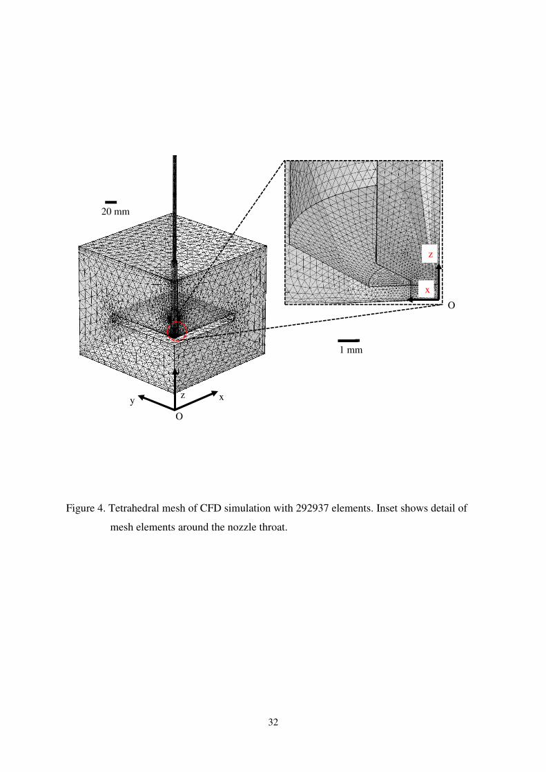
as a quadrant in 3-D and the final solution mesh used in the simulations is shown in Figure 4.
The computer memory limited the number of mesh elements to approximately 3×10⁶. The
highest pressure and velocity gradients occur under the nozzle rim and along the lip, and the
mesh element density was greatest in these regions. Tetrahedral mesh elements were specified
using the software’s mesh generation package. The mesh patterns for ejection and suction were
quite similar, except that there is a recirculation zone in the expanding part of nozzle in suction
mode. More mesh elements were specified in these regions as a result. The computing time for
each simulation varied from several minutes to a couple of hours.

8
4.1.3 CFD validation
The simulation results were checked by comparing predicted and measured pressure drops, as
well as mass conservation. The inlet and outlet mass flow rates were compared for all values
studied (0.17 – 0.90 g/s, in ejection and suction mode) and gave good agreement. Increasing
the number of mesh elements did not affect the mass balance noticeably, but did give rise to
differences in the pressure drop and thus the calculated Cd values. Mesh elements were added
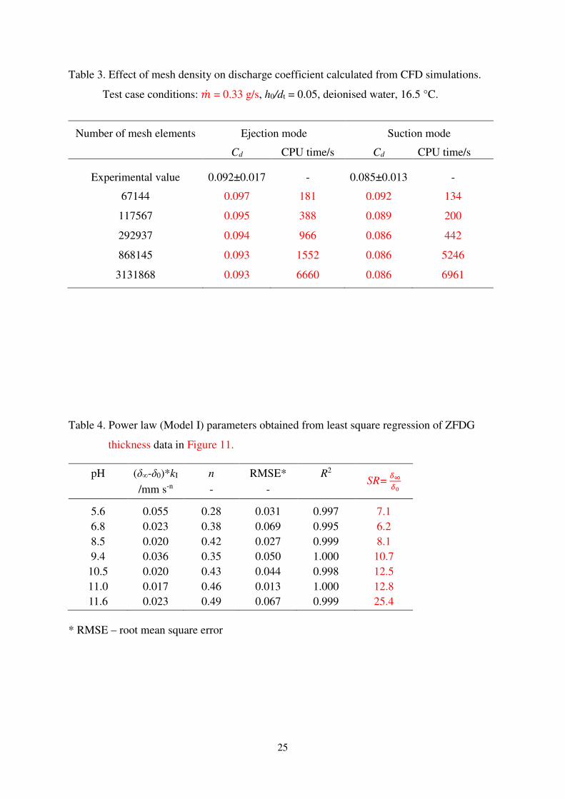
progressively in the regions of high shear rate. Table 3 shows that Cd approaches an asymptote
as the number of mesh elements was increased, at the cost of computational effort. The
predicted values of Cd differ between ejection and suction mode, which is related to the
presence of the recirculation zones and larger regions of higher velocity in the latter mode.
Similar results were reported by Yang et al.4 in their simulations which employed cylindrical,
2-D geometries. The agreement between the simulated and experimental values in Table 3 is
good, while the difference in magnitude between the simulated Cd values in suction and
ejection matches the difference in the experimental values.
The solutions reported here were obtained by running a series of simulations with progressively
lower viscosity, using the converged solution from one to start the next test. The CPU time for
ejection mode calculations is larger than for suction mode when fewer mesh elements are used
because the embedded solver in COMSOL takes longer to resolve the jet in the region
underneath the nozzle for a low viscosity liquid. By comparison, the difference is relatively
small when the largest number of mesh elements was used.
4.1.4 Surface shear stress
The CFD simulations allow the shear stress imposed by the ZFDG flow on the surface being
studied to be estimated. This can then be related to the stresses required to cause cohesive
failure4, and the adhesion between the layer and the surface6. Chew et al. 7 showed that the
shear stress directly under the nozzle rim, τw, can be estimated from the results for laminar
radial flow between two parallel discs, viz.
= = >?�����@ (9)
where x is the distance from the nozzle centreline. The largest value of τw occurs at the inner
rim of the nozzle, i.e. x = 0.89 mm for the nozzle employed in these tests. This analytical result

9
is compared with the shear stress distributions obtained from the simulations in the
Supplementary Material.
4.2 Swelling Dynamics
Three quantitative models are used in this work to characterise the PVA and gelatin layer
swelling kinetics.
I Power law mass uptake
Ritger and Peppas8 reviewed polymer swelling behaviour and reported that swelling kinetics
are often described by a simple power law relationship, viz.
� = �ABCDE (10)
where m is the solvent taken up after time t, m∞ is the amount taken up at swelling equilibrium,
t is the time immersed, kI is a kinetic constant and n is the ‘diffusion index’. Assuming that the
solvent (water) uptake is uniformly distributed over the surface and the surface area and gelatin
density do not change during the swelling process, the increase in mass is proportional to the
change in thickness of the layer. This gives
# " = ( A# ")BCDE (11)
where δ0 is the initial dry thickness, A is the final thickness and is the layer thickness at
time t. Regression fitting of swelling profiles (plots of δ against t) is used to identify the
parameters kI (δ∞-δ0) and n: the latter indicates the type of swelling mechanism, e.g. n = 0.5
being interpreted as Case I or ‘Fickian’ behaviour and n = 1 as Case II or chain relaxation.
II Second order swelling
Schott9 proposed this model to fit the swelling dynamics observed with gelatin and cellulose in
aqueous media. The rate of swelling is assumed to be proportional to
(i) The swelling capacity (fractional amount of swell), given by (m∞ - m)/m∞, at time t, and
(ii) The internal specific boundary area, Sint, representing the sites in polymer networks that
have not yet interacted with water at time t but will hydrate and swell in due course,
given by
FGE+ = B′ -�I9��I
4 (12)
where B′ is a geometrical factor accounting for interchain hydrogen bonds. Polymeric networks
are held together by hydrogen bonds and other attractive forces between adjacent chains. When

10
solvent penetrates into the structure, these bonds are broken and new linkages are formed,
particularly if the solvent promotes charge formation on the polymer. If there is charge
formation, the polymer network expands to accommodate the influx of solvent caused by
osmotic pressure. Sint is a significant parameter in this swelling model. The overall rate of
solvent uptake (swelling) is then given by
�J�+ = B -�I9�
�I4 FGE+ = BB′(�I9�
�I)� = BCC(�A #�)� (13)
where BCC = KKL�I�.
Integrating from the initial condition, m = m0 at t = 0, yields
�(D) = �MN�IKOO+(�I9�M)PNKOO+(�I9�M)
(14)
Assuming uniform density and thickness across the layer gives
= )MN)IKOO+()I9)M)PNKOO+()I9)M)
(15)
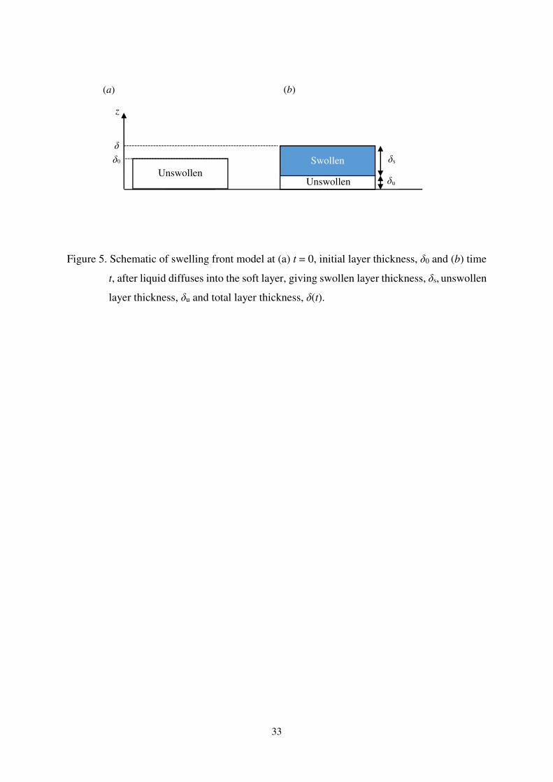
III Swelling front model
In this case the polymer is assumed to swell instantaneously in the presence of an undefined
level of solute, giving rise to a swelling front dividing a swollen region wherein the solute is
present and a region into which the solute will move (see Figure 5). The rate of ingress of the
swelling front is assumed to be controlled by Fickian diffusion or another process which
follows similar dynamics. The thickness of the gel layer at time t can written as the sum of the
thicknesses of the swollen and unswollen layers (δs and δu, respectively):
(D) = * + Q (16)
The overall rate of layer growth is given by
�R�+ =
�)��+ + �)'
�+ (17)
Defining a swelling ratio, α, as
α = # �)'�)�
(18)
Equation (17) becomes,
�R�+ = -1 # P
S4�)'�+ (19)

11
If the progress of the swelling front is controlled by Fickian diffusion for a dilute species, one
can write
�)'�+ = #T �)�
�+ = KUUU)'
(20)
where kIII is related to the diffusivity of the species. Integrating from t = 0, *= 0 gives
* = �2BWWWD (21)
Rearrangement gives
∆δ = δ # " = -1 # PS4�2BWWWD (22)
The layer thickness is expected to increase with t 0.5, and to stop swelling when δ = αδ0.
5. Results and Discussion
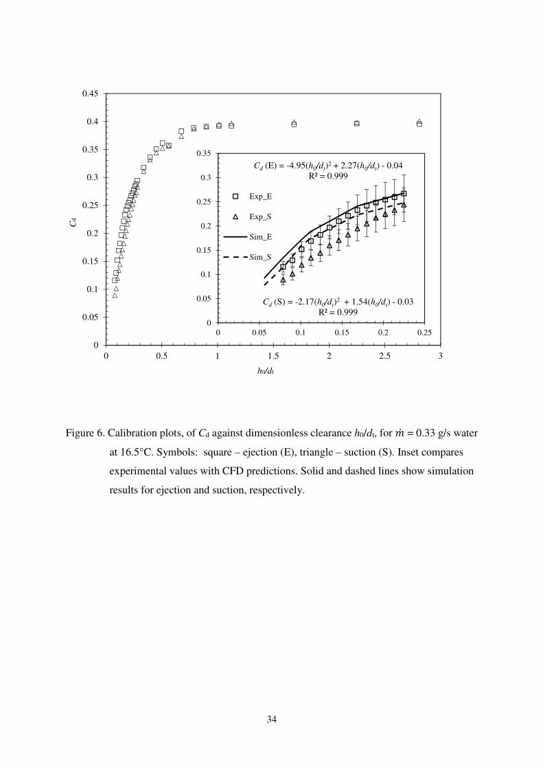
5.1 ZFDG Calibration and Accuracy
Calibration tests were performed at room temperature with deionised water as the gauging
liquid. The sets of calibration plots (Cd vs h0/dt) obtained using a flowrate of 0.33 g/s in Figure
6 show similar behaviour to that reported previously.2, 5 For a fixed flow rate, ∆P is greatest
and Cd smallest when the nozzle is close to the surface. Cd increases with increasing h/dt and
approaches an asymptote at large h/dt; in this case Cd ~ 0.40. The value of the asymptote
depends on Ret. In this pressure mode gauging configuration, lower Cd values are preferred as
the ∆P measured for a given flow rate is larger. The error bar associated with the uncertainty
in the pressure transducer measurement becomes more significant at larger h/dt. At small h/dt
values the shear stress imposed by the gauging liquid on the surface is large and there is thus a
trade-off between measurement accuracy and measurement reliability.10
The range of h0/dt values in the inset in Figure 6 represent the optimal range of gauging
conditions: the calibration plot is usefully close to linear in this region. The inset shows that
there is good agreement between the experimental Cd values and those predicted by the CFD
simulations in ejection mode. The measured suction mode values are noticeably smaller than
the simulation values, which is attributed to limitations in the pressure transducer used. The
trend is, nevertheless, reproducible and allows thickness measurements to be made with
confidence.
12
The main uncertainties in measurements arise from the accuracy in determining the nozzle–
substrate clearance, h0, since ∆P is very sensitive to lower values of h. The accuracy of the
mass flow measurements is good (less than 1% error). The pressure transducer uncertainty is
reduced by amplification and filtering to increase the signal to noise ratio.
The accuracy was checked by comparing ZFDG measurements of the thickness of layers of
waterproof tape which could be measured independently with a digital micrometer
(Mitutoyo®). A typical tape thickness was 900 µm. ZFDG measurements were performed on
the test layer at three flow rates (0.17 – 0.50 g/s) and the agreement with the micrometer value
compared at each h/dt. These tests indicated that the best agreement was obtained with h/dt near
0.10, with an uncertainty of ± 10 µm. For a given flow rate, this corresponds to a given ∆P
value: in practice, the nozzle is moved towards the surface until the pressure transducer reads
this value, and the layer thickness can then be determined from Equation (3).
Dynamic thickness measurements on gelatin were performed using a flowrate of 0.33 g/s,
changing h/dt from 0.20 to 0.05 initially by increments of 0.01. Suction mode gave an accuracy
of ±10 µm whereas ejection mode was less accurate, at ± 20 µm. The best resolution achieved
was ~± 5 µm for measurements at 0.09 <h/dt <0.11. When the syringe movement is initiated
there is a brief disturbance in ∆P which lasted less than 1 s. These transients were eliminated
from the data before processing.
5.2 Swelling of PVA layers
PVA layers were immersed in deionised water for about 5 hours. ZFDG measurements were
taken continuously, with ejection and suction stages each lasting about 2 s. Figure 7(a) shows
that swelling was still occurring at the conclusion of the test, at which point the liquid content
had reached 28 wt% (cf. initial value of 15.8 wt%). The thickness measurements obtained from
gravimetric testing are plotted alongside the ZFDG measurements and show very good
agreement compared with the suction mode values: the ejection mode data also agree within
the measurement uncertainty. The micrometer measurements are expected to underestimate the
thickness at longer times due to the elasticity of the layer when compressed by the micrometer
stub. Use of ZFDG to measure soft solids swelling in situ, making substantially more thickness
measurements, is thereby demonstrated. Moreover, ZFDG avoids the challenges faced when

13
dealing with non-ambient temperatures, hazardous solvents or the requirements of aseptic
operation.
There is a noticeable disagreement between ejection and suction measurements, although the
difference lies within the measurement uncertainty. The difference between suction and
ejection appears to be reset periodically, which corresponds to the time when the nozzle was
moved upwards. This difference is attributed to deformation of the layer by the shear stresses
imposed by the flow: the CFD simulations indicated that the largest τw values ranged from 2
to 20 Pa in these tests. The PVA material is viscoelastic: the consistency of the trends in
successive suction and ejection measurements suggest that the interaction is primarily elastic
and characterised by a short timescale. Interactions between the ZFDG liquid flow pattern and
the layer is the subject of ongoing work.
Swelling in the PVA layer is expected to be driven by diffusion and chain relaxation. The
absence of an equilibrium swelling state means that the data cannot be fitted to Model II. The
ZFDG data are replotted in Figure 7(b) as ∆δ vs t for comparison with Model I and show a
reasonable fit to the suction data. The diffusion index, n, is close to 0.7 and indicates that this
is an example of anomalous transport, combining Fickian diffusion with polymer relaxation
due to internal stresses arising from swelling of the polymer. 11 For the anomalous transport,
relaxation rate is a function of the balance of rigidity/flexibility, the degree of cross-linking,
the length of side chains and pH.12 The value of 0.7 indicates that polymer stretching, to
accommodate the influx of liquid, is not instantaneous.
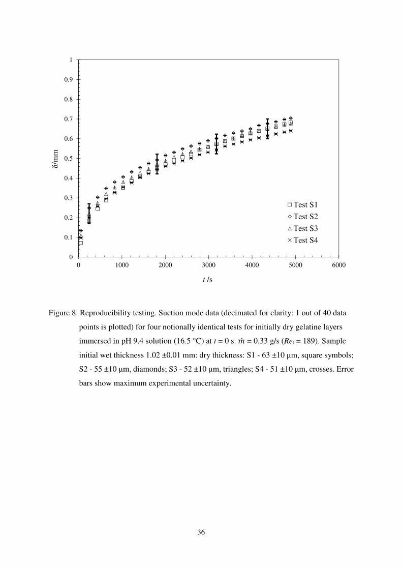
5.3 Swelling of gelatin
The swelling of gelatin layers with an initial dry thickness of 50 - 80 µm was studied at various
pH conditions at room temperature. The current ZFDG configuration does not allow the nozzle
to scan the surface13 and thereby collect several data sets from each sample, so several samples
(at least four) were tested at each condition in order to gauge the variability between samples.
Figure 8 shows acceptably good intra-sample reproducibility for notionally identical
experiments at pH 9.4. Ejection mode profiles showed the same behaviour, whereas there were
noticeable differences between the two modes for the PVA layers in Figure 7. Standard
deviations of 40 µm and 34 µm were obtained using ejection and suction modes, respectively.
14
The initial loading of the sample and initiating the flow took about 30 s, during which there is
a fast hydration step driven by diffusive, chemical and electrostatic interactions.14 The layer is
then approximately 100 µm thick. Thereafter the rate of swelling decreases: Gordon et al.15
observed similar behaviour using a scanning FDG system, and reported that the swollen layer
thickness approached an asymptote after 4 hours, i.e. at longer times than the 5000 s duration
of these tests.
The impact of the stress imposed by the gauging flow was investigated by using different flow
rates (m� = 0.33 – 0.67 g/s) in notionally identical tests. Figure 9 shows the evolution of gelatin
layer thickness at pH 6.8 (tap water), determined in suction mode. There is a consistent, small
difference in measured thickness, with the largest value recorded for the highest flow rate and
thus suction stress which would cause the layer to swell. This confirms that the gel has an
elastic response to stress. Further work could include systematically switching between suction
and ejection to determine the mechanical properties of the interface. This result indicates that
it is important to use consistent suction or ejection conditions when comparing factors,
particularly when collecting data for quantitative modelling.
ZFDG measurements showed generally good agreement with gravimetric testing: this is
discussed in detail below.
Effect of pH
Alkaline solutions are generally cheap cleaning agents that can break down protein layers
through the action of hydroxyl ions.16 The swelling of gelatin in alkali at lower pH is governed
by osmotic pressure differences arising between the protein phase and the external solution.17
As a protein, however, the biopolymer contains ionisable functional groups. When there is
electrostatic repulsion among the groups, it leads to chain expansion which can affect the
macromolecular chain relaxation.18 The swelling mechanism then becomes more relaxation-
controlled. Ionisation is expected to have an influence when the pH in the layer approaches the
pKa values for the amine groups in gelatin: for glycine (21 wt% of total), at 9.6; for glutamic
acid (10 wt%), at 9.7; for proline (12 wt%), at 10.6; and for hydroxyproline (12 wt%), also at
10.6.19

15
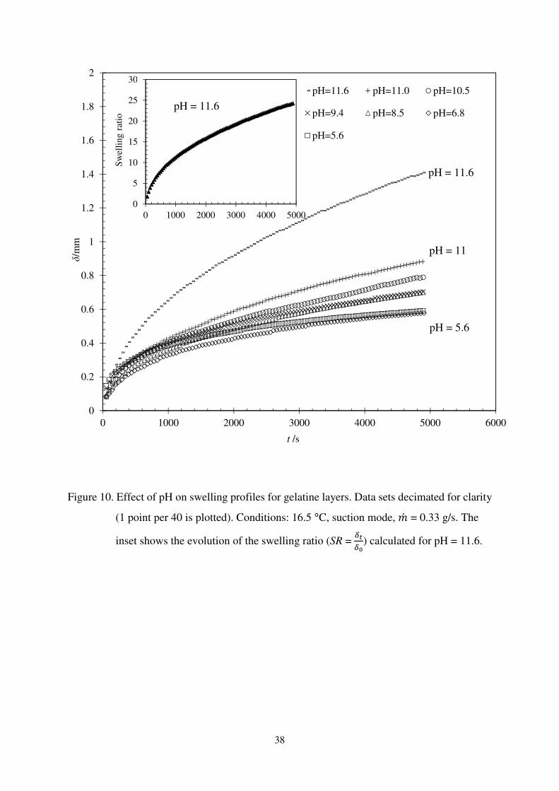
Figure 10 shows swelling profiles recorded for pH ranging from 5.6 to 11.6. In all cases the
rapid initial hydration phase is completed within 200 s and is followed by slower swelling.
There is a noticeable effect of the strongest alkali after 8 min (~ 500 s), with a swelling rate
about twice that of the other cases. After 5000 s the extent of swelling at pH 11.6 was about
50% greater than that at pH 11. By comparison, the extent of swelling at pH 11 after 5000 s (~
0.8 mm in Figure 10) was about 50% greater than that at pH 5.6 (~ 0.55). Gordon et al.15
reported similar differences between pH 11.6 and 9.4 (achieved in their studies using 0.03 M
buffer solutions). The large increase in swelling at pH 11.6 is attributed to deprotonation of the
amine groups on proline and hydroxyproline driving charge repulsion within the layer. It is
noticeable that the amount of extra repulsion was relatively weak at pH 11. This could be due
to depletion of the H+ concentration as the solvent diffuses into the layer and is consumed in
protonation steps: a high concentration is needed to drive the reaction to completion.20
Comparison with gravimetric tests
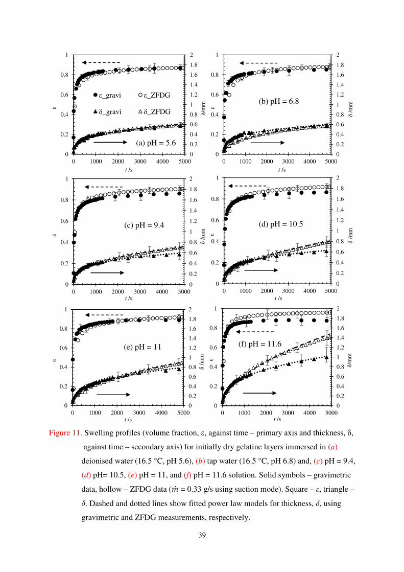
Figure 11 presents the results obtained from ZFDG and gravimetric testing on notionally
identical gelatin layers immersed in deionised and tap water (pH 5.6 and 6.8, respectively,
differing due to the presence of dissolved CO2), and alkaline solutions with pH 8.5 - 11.6. The
data are presented as the thickness, δ (measured directly by micrometer or ZFDG) and volume
fraction of solution ε. The latter was calculated assuming that the density of water and polymer
are approximately equal: for gravimetric testing, εg is given by equation (4) and for ZFDG
studies, εZ is given by equation (5). The initial gravimetric voidage is calculated from
$ = 1 #Z��[
\��[∗(^��_ )
)��[ (23)
where d is the disc diameter. The thickness measurements show very good agreement between
the two techniques, within experimental uncertainty, until higher pH conditions. At pH 11.6
there is an extensive swelling and the difference in δ values is significant. This consistent
difference is attributed to the compression imposed by the micrometer stub measurement
action: the more highly swollen layer is expected to be weaker and thus less able to resist the
stub compression. At this pH the δ values collected in suction and ejection modes at longer
times differed by about 10%, indicating some elasticity in the highly swollen layer.

16
Both techniques show that ε increases rapidly initially, from about 20% to 80% within 8 min,
followed by slow swelling to an asymptotic value of around 90%. The initial rate of solution
uptake is greater at higher pH and the asymptote is approached more quickly. There is a
difference between εg and εZ values at higher pH, which is thought to arise from mass loss when
handling and drying the highly swollen layer as well as dissolution of the gelatin. The layers
all followed the same relationship between (overall) voidage and layer thickness, shown in
Figure 12, indicating that pH was determining the rate at which the material swelled.
Modelling swelling
Plotted alongside the ZFDG thickness data in Figure 11 are the lines of best fit obtained for the
power law model, Equation (10) to the gravimetric data. Similarly good agreement, albeit
yielding different model parameters, was obtained by fitting Equation (11) to the ZFDG data
sets. The parameters obtained by fitting suction mode ZFDG data are summarised in Table 4.
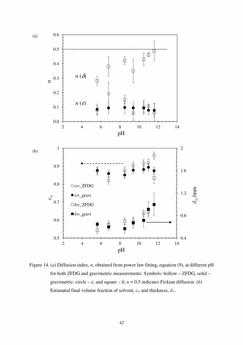
The diffusion index, n, increases with increasing pH and approaches 0.5, the value associated
with Fickian transport, at higher pH. This transition between ‘sub Fickian’ behaviour, which is
dependent on the relative contribution of penetrant diffusion and polymer relaxation, and
Fickian with increasing pH, is attributed to differences between the solvent penetration rate and
the polymer chain relaxation rate.21. The swelling ratio, calculated at the end of the test is also
reported in Table 4 and increases by a factor of 3.6 across the pH range.
Figure 13 shows an example of the fit of the three swelling models to the experimental data
obtained for gelatine layers contacted with pH 11.6 solution. The models were fitted to data
after the hydration stage: Models I and II give reasonable agreement with the suction and
ejection mode data over the time period studied (R2 > 0.99), whereas Model III did not give
good agreement initially (t < 360s). There is a systematic difference between suction and
ejection thickness measurements at this pH, which is attributed to elasticity in the layer.
Fitting the power law model, Equation (11) to the data (Figure 13(a)) gave a diffusion index of
n = 0.49 (see Table 4). The second order model (Equation 15, (Figure 13(b)) shows good
agreement except in the early stage of (t < 200 s), where it over-predicts the layer thickness:
this is likely due to hydration. The equilibrium thickness of the gelatine layer, δ∞, can be
estimated from the model parameters, from
17
A,`*+ = )I∗()I9RM)∗KOO()I9RM)∗KOO
(24)
giving δ∞ = 2.36 ±0.02 mm and 2.27 ±0.02 mm for the ejection and suction case, respectively.
This final thickness, of approximately 2.3 mm, is four times the initial wet thicknesses of the
layers (prepared at pH 6.8), indicating that the polymer wants to adopt a more open
configuration at the higher pH – which is consistent with repulsion between charged chains.
At pH 11.6 the power law index is 0.49 and the swelling front model, (Figure 14(c), Equation
(22)) is then of similar form and gave a reasonable fit. kIII gives an order of magnitude estimate
of a Fickian diffusion coefficient as 3.8×10⁻¹⁰ m2/s. This is comparable with the average
diffusivity of hydroxyl ion in a whey protein gel at pH 12.2 solution of 1.15×10⁻⁹ mm2/s
reported by Mercadé-Prieto & Chen.22
The effect of pH on the power law model parameters is summarised in Figure 14. The ‘diffusion
index’ n differed from 0.5 at pH values other than 11.6 so the fit of the swelling front model
was poorer (data not reported). There is a systematic effect of pH on ε∞ and δ∞, in accordance
with charge-induced swelling at pH values above 9.4.
ZFDG demonstrates significant advantages over gravimetric testing: (i) the samples do not
have to be removed from solution; (ii) more frequent measurements can be made (and with
scanning, more sites tested), (iii) softer layers can be studied reliably; and (iv) measurements
are not influenced by the user’s experimental technique. Furthermore, ZFDG tests can be
conducted at other temperatures (and pressures) readily, rendering it a powerful tool for
studying fouling or cleaning.
6. Conclusions
The concept of automated zero discharge fluid dynamic gauge has been demonstrated. The
ability to operate with a fixed volume of liquid has advantages when using hazardous liquids
or reagents with limited availability. The experimental calibration curves showed similar
behaviour between suction and ejection stages. This difference was evident in CFD simulations
and there was reasonable agreement between experimental and simulation Cd values.

18
Calibration testing identified a useful measurement range, 0.05 < h0/dt < 0.20, with a maximum
resolution of ± 5 µm, and accuracy of ± 10 µm for the thickness measurements. CFD
simulations indicated that the shear stress imposed on the surface being gauged varied more
noticeably in ejection mode, so suction mode should be favoured for measuring thicknesses of
deformable layers at a given flow rate.
The swelling characteristics of layers prepared from PVA glue in water and thinner gelatin
layers at different pH were studied. ZFDG measurements gave good agreement with simple
(and more time-consuming) gravimetric methods. The PVA layers exhibited swelling of the
‘anomalous transport’ type. Gelatin behaviour depended on pH, with the diffusion index of a
simple power law model increasing with pH. These results are consistent with previous studies.
Acknowledgements
Development of the ZFDG concept was supported by the Royal Society’s Paul Instrument
Fund. Funding from Fitzwilliam College for Shiyao Wang is also gratefully acknowledged.

19
Reference
(1) Tuladhar, T.R.; Paterson, W.R.; Macleod, N.: Wilson, D.I., Development of a
novel non-contact proximity gauge for thickness measurement of soft deposits and its
application in fouling studies. Can. J. Chem. Eng. 2000, 78, 935-947.
(2) Chew, J.Y.M.; Cardoso, S.S.S.; Paterson, W.R.; Wilson, D. I. CFD studies of
dynamic gauging. Chem. Eng. Sci. 2004, 59(16), 3381–3398.
(3) Chew, J.Y.M.; Tonneijk, S.J.; Paterson, W.R.; Wilson, D.I. Mechanisms in
the solvent cleaning of emulsion polymerization reactor surfaces. Ind. Eng. Chem. Res. 2005,
44(13),4605-4616.
(4) Yang, Q.; Ali, A.; Shi, L.; Wilson, D.I. Zero discharge fluid dynamic gauging
for studying the thickness of soft solid layers. J. Food Eng. 2014, 127, 24–33.
(5) Gordon, P.W.; Brooker, A.D.M.; Chew, J.Y.M.; Wilson, D.I.; York, D.W. A
scanning fluid dynamic gauging technique for probing surface layers. Measurement Sci. and
Tech. 2010, 21(8), 85103.
(6) Saikhwan, P.; Chew, J.Y.M.; Paterson, W.R.; Wilson, D.I. Swelling and its
suppression in the cleaning of polymer fouling layers. Ind. Eng. Chem. Res. 2007, 46(14),
4846-4855.
(7) Chew, J.Y.M.; Höfling, V.; Augustin, W.; Paterson, W.R.; Wilson, D.I. A
method for measuring the strength of scale deposits on heat transfer surfaces. Dev. Chem. Eng.
Mineral Proc. 2005, 13(1/2), 21-30.
(8) Ritger, P.L.; Peppas, N.A. A simple equation for description of solute release II. Fickian
and anomalous release from swellable devices. J. Controlled Release 1987, 5, 37–42.
(9) Schott, H. Swelling kinetics of polymers. J. Macromolecular Sci., Part B:Physics 1992,
31:1, 1-9.
(10) Salley, B.; Gordon, P.W.; McCormick, A.J.; Fisher, A.C.; Wilson, D.I. Characterising
the structure of photosynthetic biofilms using fluid dynamic gauging. Biofouling 2012, 28:2,
159–173.
(11) Thomas, N.L.; Windle, A.H. A deformation model for case II diffusion. Polymer 1980,
21, 613–619.
(12) Ganji, F.; Vasheghani-Farahani, S.; Vasheghani-Farahani, E. Theoretical description
of hydrogel swelling: A review. Iranian Polymer J. 2010, 19(5), pp.375–398.
(13) Gordon, P.W.; Schöler, M.; Föste, H.; Helbig, M.; Augustin, W.; Chew, Y.M.J.; Scholl,
S.; Majschak, J-P.; Wilson, D.I. A comparison of local phosphorescence detection and fluid
dynamic gauging methods for studying the removal of cohesive fouling layers: effect of layer
roughness, Food Bioprod. Proc. 2014, 92, 46–53.
20
(14) Ofner III, C. M.; Schott, H. Swelling studies of gelatin I: Gelatin without additives. J.
Pharma. Sci. 1986, 75, 790–796.
(15) Gordon P.W.; Brooker A.D.M.; Chew Y.M.J.; Letzelter, N.; York D.W.; Wilson D.I.
Elucidating enzyme-based cleaning of protein soils (gelatine and egg yolk) using a scanning
fluid dynamic gauge, Chem. Eng. Res. Des. 2012, 90, 162-171.
(16) Lelieveld, H. L. M. Hygiene in Food Processing, 2003,Woodhead Publishing Series in
Food Science, Technology and Nutrition
(17) Bowes, J.H.; Kenten, R.H. The swelling of collagen in alkaline solutions. 1. Swelling
in solutions of sodium hydroxide. Biochem. J., 1950, 46(1), 1–8.
(18) Gierszewska-Drużyńska, M.; Ostrowska-Czubenko, J., Mechanism of water diffusion
into noncrosslinked and ionically crosslinked chitosan membranes. 2011, XVII Seminar and
Workshop "New Aspects of the Chemistry and Applications of Chitin and its Derivatives",
Warsaw.
(19) Stevens, P.V. Gelatine. Food Australia 1992, 44(7), 320-324.
(20) Mercadé-Prieto, R; Paterson, W. R.; Chen, X.D.; Wilson, D. I. Diffusion of NaOH into
a protein gel. Chem. Eng. Sci. 2008, 63(10), 2763–2772.
(21) Dengre, R.; Bajpai, M.; Bajpai, S.K. Release of Vitamin B12 from poly (N-vinyl-2-
pyrrolidone)-crosslinked polyacrylamine hydrogels: a kinetic study, J. Appl. Polym.Sci. 2000,
76, 1706-1714.
(22) Mercadé-Prieto, R.; Chen, X.D. Dissolution of whey protein concentrate gels in alkali.
AIChE J., 2006, 52(2), 792–803.

21
Nomenclature
Roman
Cd Fluid discharge coefficient -
d Disc diameter m
di Inner diameter m
dt Diameter of nozzle throat m
do Outer diameter m
h Nozzle-layer clearance m
h0 Nozzle-substrate clearance m
H Height of liquid immersed in tank m
k Rate constant -
kI Rate constant for power law model -
kII Rate constant for second order -
kIII Rate constant for swelling front model -
m Mass kg
ms Initial dry mass of model layers kg
mt Mass in time t kg
m∞ Mass in the equilibrium state kg
�� Mass flow rate of gauging liquid kg/s
n Diffusion index -
∆P Differential pressure (∆Pdyn – ∆Pstatic) Pa
r Radial co-ordinate m
R2 Coefficient of determination -
Ret Reynolds number at nozzle throat -
Sint Internal specific boundary area m2
t Time s
vm Mean velocity m/s
W Width m
we Nozzle rim thickness m
wr Nozzle rim width m
x Horizontal coordinate m
z Vertical coordinate m

22
Greek
α Swelling ratio -
δ Layer thickness m
δs Swollen layer thickness m
δt Swollen layer thickness at time t m
δu Unswollen layer thickness m
δ0 Initial dry layer thickness m
δ∞ Final layer thickness m
δ∞, est Estimated final layer thickness m
ε Water/solvent volume fraction -
εg Water/solvent volume fraction in gravimetric measurement -
εs Initial water/solvent volume fraction -
εZ Water/solvent volume fraction in ZFDG -
ε∞ Final water/solvent volume fraction -
θ Nozzle converging angle °
ρ Density of gauging liquid kg/m3
τw Wall shear stress Pa
µ Liquid viscosity Pa s
Acronyms
CFD Computational fluid dynamics
PT Pressure transducer
PVA Poly vinyl acetate
RMSE Root mean-square deviation
ZFDG Zero (net) discharging fluid dynamic gauging

23
List of Table Captions:
Table 1. CFD simulation dimensions and fluid parameters
Table 2. Boundary conditions in CFD simulations (see Figure 3 for labelled locations)
Table 3. Effect of mesh density on discharge coefficient calculated from CFD simulations.
Test case conditions: �� = 0.33 g/s, h0/dt = 0.05, deionised water, 16.5 °C.
Table 4. Power law (Model I) parameters obtained from least square regression of ZFDG
thickness data in Figure 11.

24
Table 1. CFD simulation dimensions and fluid parameters
Parameters Value
dt 1.78 mm
di 4 mm
do 8 mm
H 120 mm (liquid depth)
W 280 mm
L 310 mm
μ 1.12 mPa s
ρ 997.3 kg/m3
temperature 16.5 °C
Table 2. Boundary conditions in CFD simulations (see Figure 3 for labelled locations)
Boundary Description Boundary condition
A Axis of symmetry No radial flow, i.e. vx =0
B Gauging nozzle tube Fully developed laminar flow at end, vx =0
�� is defined by syringe pump, with
a@ = ��������
(1 # �@����) (ejection)
a@ = 9��������
(1 # �@����) (suction)
C, D Wall: no slip and impermeable vx = 0; vz = 0
E Open boundary Parallel streamlines, p = 0
25
Table 3. Effect of mesh density on discharge coefficient calculated from CFD simulations.
Test case conditions: �� = 0.33 g/s, h0/dt = 0.05, deionised water, 16.5 °C.
Number of mesh elements Ejection mode Suction mode
Cd CPU time/s Cd CPU time/s
Experimental value 0.092±0.017 - 0.085±0.013 -
67144 0.097 181 0.092 134
117567 0.095 388 0.089 200
292937 0.094 966 0.086 442
868145 0.093 1552 0.086 5246
3131868 0.093 6660 0.086 6961
Table 4. Power law (Model I) parameters obtained from least square regression of ZFDG
thickness data in Figure 11.
pH (δ∞-δ0)*kI
/mm s-n
n
-
RMSE*
-
R2 SR=)I)M
5.6 0.055 0.28 0.031 0.997 7.1
6.8 0.023 0.38 0.069 0.995 6.2
8.5 0.020 0.42 0.027 0.999 8.1
9.4 0.036 0.35 0.050 1.000 10.7
10.5 0.020 0.43 0.044 0.998 12.5
11.0 0.017 0.46 0.013 1.000 12.8
11.6 0.023 0.49 0.067 0.999 25.4
* RMSE – root mean square error

26
List of Figure captions
Figure 1. Schematic elevation of ZFDG geometry. Nozzle dimensions: θ = 54°, dt = 1.78 mm,
di = 4 mm, we = 0.2 mm, wr = 1.32 mm. Dotted streamline – ejection mode; dashed
streamline – suction mode (showing flow recirculation).
Figure 2. (a) Schematic view of ZFDG test rig; photographs of (b) ZFDG test rig with (c)
1.78 mm i.d. nozzle throat. Labels: A - syringe pump; B - stepper motor; C -
pressure transducer (PT); D – nozzle.
Figure 3. Boundaries in CFD simulations. Label descriptions given in Table 2. O is the origin
of the Cartesian coordinate frame.
Figure 4. Tetrahedral mesh of CFD simulation with 292937 elements. Inset shows detail of
mesh elements around the nozzle throat.
Figure 5. Schematic of swelling front model at (a) t = 0, initial layer thickness, δ0 and (b) time
t, after liquid diffuses into the soft layer, giving swollen layer thickness, δs, unswollen
layer thickness, δu and total layer thickness, δ(t).
Figure 6. Calibration plots, of Cd against dimensionless clearance h0/dt, for �� = 0.33 g/s water
at 16.5°C. Symbols: square – ejection (E), triangle – suction (S). Inset compares
experimental values with CFD predictions. Solid and dashed lines show simulation
results for ejection and suction, respectively.
Figure 7. (a) Swelling of PVA glue film immersed in deionised water (pH = 5.6, 16.5 °C) with
�� = 0.50 g/s. Gravimetric results are shown in black hollow circles. Representative
error bars plotted. Symbols: square – ejection (E), triangle – suction (S). Inset
compares experimental values with CFD predictions. Solid and dashed lines show
simulation results for ejection and suction, respectively. δfinal is the maximum
thickness measured. (b) Fit of power law model (Equation 11) to where Δ = (t) –
", dotted line – ejection, and dashed line – suction.

27
Figure 8. Reproducibility testing. Suction mode data (decimated for clarity: 1 out of 40 data
points is plotted) for four notionally identical tests for initially dry gelatine layers
immersed in pH 9.4 solution (16.5 °C) at t = 0 s. �� = 0.33 g/s (Ret = 189). Sample initial
wet thickness 1.02 ±0.01 mm: dry thickness: S1 - 63 ±10 µm, square symbols; S2 - 55
±10 µm, diamonds; S3 - 52 ±10 µm, triangles; S4 - 51 ±10 µm, crosses. Error bars show
maximum experimental uncertainty.
Figure 9. Swelling profiles of gelatine layers with initial thickness ~ 80 ±10 µm obtained with
different gauging flowrates. pH 6.8 (tap water), suction mode.
Figure 10. Effect of pH on swelling profiles for gelatine layers. Data sets decimated for clarity
(1 point per 40 is plotted). Conditions: 16.5 °C, suction mode, �� = 0.33 g/s. The inset
shows the evolution of the swelling ratio (SR =)�)M) calculated for pH = 11.6.
Figure 11. Swelling profiles (volume fraction, ε, against time – primary axis and thickness, δ,
against time – secondary axis) for initially dry gelatine layers immersed in (a)
deionised water (16.5 °C, pH 5.6), (b) tap water (16.5 °C, pH 6.8) and, (c) pH = 9.4,
(d) pH= 10.5, (e) pH = 11, and (f) pH = 11.6 solution. Solid symbols – gravimetric
data, hollow – ZFDG data (�� = 0.33 g/s using suction mode). Square – ε, triangle –
δ. Dashed and dotted lines show fitted power law models for thickness, δ, using
gravimetric and ZFDG measurements respectively.
Figure 12. Evolution of liquid volume fraction against layer thickness for (a) ZFDG and (b)
gravimetric measurements. Legend in (a) indicates pH.
Figure 13. Comparison of swelling models with ZFDG experimental data for gelatine layers at
pH 11.6, 16.5 °C. (a) power law, equation (9); (b) Model II, equation (13); (c) swelling
front, equation (20). Data decimated for clarity. Symbols: ejection – circle, solid line;
suction – triangle, dashed line. Initial dry thickness 58 ±10 µm, �� = 0.33 g/s.
Figure 14. (a) Diffusional indices, n, from power law fitting, equation (9), at different pH for
both ZFDG and gravimetric measurements. Symbols: hollow – ZFDG, solid –

28
gravimetric; circle – ε, and square – δ; n = 0.5 indicates Fickian diffusion. (b) Estimated
final volume fraction of solvent, ε∞ and thickness, δ∞.
Supplementary Figure:
Figure S1. Shear stress imposed on the surface being gauged, from CFD calculations.
Conditions: �� = 0.33 g/s (deionised water, 16.5 °C). Hollow symbols. Left–
ejection, solid symbols, right – suction. Lines show analytical solution (denoted
‘A’) assuming radial flow between nozzle rim and substrate (Equation (9)). The
position of the inner and outer edges of nozzle rim are indicated by black vertical
dashed lines at x = ± 0.89 mm and x = ± 2.21 mm, respectively.

29
Figure 1. Schematic elevation of ZFDG geometry. Nozzle dimensions: θ = 54°, dt = 1.78 mm,
di = 4 mm, we = 0.2 mm, wr = 1.32 mm. Dotted streamline – ejection mode; dashed
streamline – suction mode (showing flow recirculation).
θ
Nozzle
cG
c+
h !"
δ
Substrate
∆P
z
de
d`
Soil

30
Figure 2. (a) Schematic view of ZFDG test rig; photographs of (b) ZFDG test rig with (c) 1.78
mm i.d. nozzle throat. Labels: A - syringe pump; B - stepper motor; C - pressure
transducer (PT); D – nozzle.
Nozzle Pressure tapping
Stage
Stepper motor
Perspex tank
Syringe pump
SubstrateLevel
(a)
C B
A
D
(b)
D
h0 dt
(c)
(a)

31
Figure 3. Boundaries in the FD simulations. Label descriptions are given in Table 2. O is the
origin of the Cartesian coordinate frame.
B
A
D
E
C C
C
C
C
z
x
W = 140 mm
H =
12
0 m
m
O
Stage
32
Figure 4. Tetrahedral mesh of CFD simulation with 292937 elements. Inset shows detail of
mesh elements around the nozzle throat.
x z
y
20 mm
1 mm
z
x
x z y
O
O
33
Figure 5. Schematic of swelling front model at (a) t = 0, initial layer thickness, δ0 and (b) time
t, after liquid diffuses into the soft layer, giving swollen layer thickness, δs, unswollen
layer thickness, δu and total layer thickness, δ(t).
(a) (b)
Unswollen
z
δ0
Unswollen δu
Swollen δs
δ
34
Figure 6. Calibration plots, of Cd against dimensionless clearance h0/dt, for �� = 0.33 g/s water
at 16.5°C. Symbols: square – ejection (E), triangle – suction (S). Inset compares
experimental values with CFD predictions. Solid and dashed lines show simulation
results for ejection and suction, respectively.
0
0.05
0.1
0.15
0.2
0.25
0.3
0.35
0.4
0.45
0 0.5 1 1.5 2 2.5 3
Cd
h0/dt
Cd (E) = -4.95(h0/dt)2 + 2.27(h0/dt) - 0.04
R² = 0.999
Cd (S) = -2.17(h0/dt)2 + 1.54(h0/dt) - 0.03
R² = 0.999
0
0.05
0.1
0.15
0.2
0.25
0.3
0.35
0 0.05 0.1 0.15 0.2 0.25
Exp_E
Exp_S
Sim_E
Sim_S

35
Figure 7. (a) Swelling of PVA glue film immersed in deionised water (pH = 5.6, 16.5 °C) with
�� = 0.50 g/s. Gravimetric results are shown in black hollow circles. Representative
error bars plotted. Symbols: square – ejection (E), triangle – suction (S). Inset
compares experimental values with CFD predictions. Solid and dashed lines show
simulation results for ejection and suction, respectively. δfinal is the maximum
thickness measured. (b) Fit of power law model (Equation 11) to where Δ = (t) –
", dotted line – ejection, and dashed line – suction.
1.6
1.65
1.7
1.75
1.8
1.85
1.9
1.95
2
2.05
2.1
0 5000 10000 15000 20000
δ/m
m
t /s
∆ = 0.008t0.648
R² = 0.971
∆ = 0.006t0.699
R² = 0.997
0
0.1
0.2
0.3
0.4
0.5
0 5000 10000 15000 20000
∆δ/m
m
t /s
δ0 = 1.66 mm
δfinal, s = 1.98 mm
Ejection
Suction
Suction
Ejection
(a)
(b)
∆ = (δ∞ - δ0)kI*tn
36
Figure 8. Reproducibility testing. Suction mode data (decimated for clarity: 1 out of 40 data
points is plotted) for four notionally identical tests for initially dry gelatine layers
immersed in pH 9.4 solution (16.5 °C) at t = 0 s. �� = 0.33 g/s (Ret = 189). Sample
initial wet thickness 1.02 ±0.01 mm: dry thickness: S1 - 63 ±10 µm, square symbols;
S2 - 55 ±10 µm, diamonds; S3 - 52 ±10 µm, triangles; S4 - 51 ±10 µm, crosses. Error
bars show maximum experimental uncertainty.
0
0.1
0.2
0.3
0.4
0.5
0.6
0.7
0.8
0.9
1
0 1000 2000 3000 4000 5000 6000
δ/m
m
t /s
Test S1
Test S2
Test S3
Test S4

37
Figure 9. Swelling profiles of gelatine layers with initial thickness ~ 80 ±10 µm obtained with
different gauging flowrates. pH 6.8 (tap water), suction mode.
0
0.1
0.2
0.3
0.4
0.5
0.6
0.7
0 1000 2000 3000 4000 5000 6000
∆δ/m
m
t /s
0.67 g/s
0.50 g/s
0.33 g/s
38
Figure 10. Effect of pH on swelling profiles for gelatine layers. Data sets decimated for clarity
(1 point per 40 is plotted). Conditions: 16.5 °C, suction mode, �� = 0.33 g/s. The
inset shows the evolution of the swelling ratio (SR =)�)M) calculated for pH = 11.6.
0
0.2
0.4
0.6
0.8
1
1.2
1.4
1.6
1.8
2
0 1000 2000 3000 4000 5000 6000
δ/m
m
t /s
pH=11.6 pH=11.0 pH=10.5
pH=9.4 pH=8.5 pH=6.8
pH=5.6
pH = 11.6
pH = 11
pH = 5.6
0
5
10
15
20
25
30
0 1000 2000 3000 4000 5000
Sw
elli
ng r
atio
pH = 11.6
39
Figure 11. Swelling profiles (volume fraction, ε, against time – primary axis and thickness, δ,
against time – secondary axis) for initially dry gelatine layers immersed in (a)
deionised water (16.5 °C, pH 5.6), (b) tap water (16.5 °C, pH 6.8) and, (c) pH = 9.4,
(d) pH= 10.5, (e) pH = 11, and (f) pH = 11.6 solution. Solid symbols – gravimetric
data, hollow – ZFDG data (�� = 0.33 g/s using suction mode). Square – ε, triangle –
δ. Dashed and dotted lines show fitted power law models for thickness, δ, using
gravimetric and ZFDG measurements, respectively.
0
0.2
0.4
0.6
0.8
1
1.2
1.4
1.6
1.8
2
0
0.2
0.4
0.6
0.8
1
0 1000 2000 3000 4000 5000
δ/m
m
ε
t /s
ε_gravi ε_ZFDG
δ_gravi δ_ZFDG
0
0.2
0.4
0.6
0.8
1
1.2
1.4
1.6
1.8
2
0
0.2
0.4
0.6
0.8
1
0 1000 2000 3000 4000 5000
δ/m
m
ε
t /s
0
0.2
0.4
0.6
0.8
1
1.2
1.4
1.6
1.8
2
0
0.2
0.4
0.6
0.8
1
0 1000 2000 3000 4000 5000
δ/m
m
ε
t /s
0
0.2
0.4
0.6
0.8
1
1.2
1.4
1.6
1.8
2
0
0.2
0.4
0.6
0.8
1
0 1000 2000 3000 4000 5000
δ/m
m
ε
t /s
0
0.2
0.4
0.6
0.8
1
1.2
1.4
1.6
1.8
2
0
0.2
0.4
0.6
0.8
1
0 1000 2000 3000 4000 5000
δ/m
m
ε
t /s
0
0.2
0.4
0.6
0.8
1
1.2
1.4
1.6
1.8
2
0
0.2
0.4
0.6
0.8
1
0 1000 2000 3000 4000 5000
δ/m
m
ε
t /s
(a) pH = 5.6
(b) pH = 6.8
(c) pH = 9.4 (d) pH = 10.5
(e) pH = 11 (f) pH = 11.6

40
Figure 12. Evolution of liquid volume fraction against layer thickness for (a) ZFDG and (b)
gravimetric measurements. Legend in (a) indicates pH.
0 0.5 1 1.5
0
0.2
0.4
0.6
0.8
1
ε
pH =5.6
pH =6.8
pH =8.5
pH =9.4
pH =10.5
pH =11
pH =11.6
0 0.5 1 1.5
0
0.2
0.4
0.6
0.8
1
δ /mm
ε
time
time
(a)
(b)
gravimetric
ZFDG

41
Figure 13. Comparison of swelling models with ZFDG experimental data for gelatine layers at
pH 11.6, 16.5 °C. (a) power law, equation (9); (b) Model II, equation (13); (c)
swelling front, equation (20). Data decimated for clarity. Symbols: ejection – circle,
solid line; suction – triangle, dashed line. Initial dry thickness 58 ±10 µm, �� =
0.33 g/s.
0
0.2
0.4
0.6
0.8
1
1.2
1.4
1.6
0 1000 2000 3000 4000 5000
δ/m
m
t /s
pH = 11.6_E
pH = 11.6_S
Power law fit_E
Power law fit_S
0
0.2
0.4
0.6
0.8
1
1.2
1.4
1.6
0 1000 2000 3000 4000 5000
δ/m
m
t /s
pH = 11.6_E
pH = 11.6_S
Second order fit_E
Second order fit_S
∆δ (E) = 0.021t0.5
R² = 0.996
∆δ (S) = 0.019t0.5
R² = 0.997
0
0.2
0.4
0.6
0.8
1
1.2
1.4
1.6
0 20 40 60 80
δ/m
m
t0.5 /s0.5
pH = 11.6_E
pH = 11.6_S
Linear (pH = 11.6_E)
Linear (pH = 11.6_S)
(a)
(b)
(c)
42
Figure 14. (a) Diffusion index, n, obtained from power law fitting, equation (9), at different pH
for both ZFDG and gravimetric measurements. Symbols: hollow – ZFDG, solid –
gravimetric; circle – ε, and square – δ; n = 0.5 indicates Fickian diffusion. (b)
Estimated final volume fraction of solvent, ε∞ and thickness, δ∞.
0.0
0.1
0.2
0.3
0.4
0.5
0.6
2 4 6 8 10 12 14
n
pH
0.4
0.8
1.2
1.6
2
0.5
0.6
0.7
0.8
0.9
1
2 4 6 8 10 12 14
δ∞
/mm
ε ∞
pH
ε∞_ZFDG
ε∞_gravi
δ∞_ZFDG
δ∞_gravi
(a)
(b)
n (δ)
n (ε)