Zero-Price Effects in Health Insurance: Evidence from Colorado

Coleman Drake, Sih-Ting Cai, David Anderson, Daniel W. Sacks

December 8, 2020

Abstract: The Affordable Care Act’s premium tax credit subsidies provide millions of eligible

enrollees with the option to purchase zero-premium health insurance plans, but millions more do

not have this option. What difference does a premium of zero make, relative to a slightly positive

one? We use regression discontinuity designs to examine zero-price effects in health insurance

coverage take-up, plan choice, and coverage duration using administrative data from Colorado’s

Health Insurance Marketplace from 2016 through 2019. Unlike previous studies, we isolate zero-

price effects from high price sensitivity near zero using rich variation from Marketplace

premium tax credits. We find no discontinuity in insurance choices when premiums increase

from to a slightly positive amount, suggesting that zero is not a special price for customers.

However, zero-premiums plans increase on-time enrollment, leading to longer coverage duration

by reducing the transaction cost of making an initial premium payment. As low-income

customers are especially sensitive to this transaction cost, making zero-premium plans available

may increase targeting efficiency.

Keywords: Health Insurance, Affordable Care Act, Zero-Price Effect, Regression Discontinuity

Acknowledgements We are grateful to the National Institute for Health Care Management (NIHCM) for their

support of this research. We also are grateful to Connect for Health Colorado and Vericred, Inc. for providing the

data for our analysis. The opinions expressed in this manuscript do not reflect those of Connect for Health Colorado

or Vericred, Inc. We are also thankful for feedback on this manuscript from Coady Wing, Tom McGuire, Rudy

Douven, Anne Royalty, Paul Shafer, Connect for Health Colorado, the Indiana University-Purdue University

Indianapolis Department of Economics, the Indiana University O’Neill School of Public and Environmental Affairs,

and participants at the 2020 APPAM Fall Research Conference.

1

1. Introduction

In 2018, 13% of enrollees in the Affordable Care Act's (ACA) Health Insurance

Marketplaces enrolled in zero-premium plans (Branham and Deleire 2019). Such plans are

available to households whose premium subsidy exceeds the premium of the cheapest plan

available to them. However, some states set premium floors above zero by requiring insurers to

cover benefits that are not eligible for subsidies. California, for example, sets a premium floor of

one dollar to provide elective abortion benefits (Salganicoff et al. 2014).

What difference does this dollar make? Standard economic theory assumes such

differences matter very little. Yet, recent policy proposals suggest policymakers believe they

matter greatly. For example, to increase health insurance coverage take-up, the Biden

presidential campaign’s health care plan would create a zero-premium public option for low-

income Americans (Biden for President 2020). On the other hand, five states have implemented

token Medicaid premiums under the ACA’s Medicaid expansion, and three others plan to do so

(Brooks, Roygardner, and Artiga 2019).

Both supporters and opponents of token premiums have an implicit theory that reducing

small health insurance premiums to zero can affect coverage choices. Such zero-price effects

occur for multiple reasons. Shampanier, Mazar, and Ariely (2007) argue that people perceive

free products as providing discontinuously higher benefits than products with positive prices.

Even absent such a psychological bias, positive prices can affect choice and coverage because

they create a hassle cost to finalize insurance purchase. In either case, zero-price effects could

increase overall enrollment in a health insurance market if zero-premium plans make insurance

coverage particularly attractive. Not requiring households to pay monthly premiums could also

increase coverage duration by reducing transaction costs such as mailing a check.

2

Zero-price effects also could affect coverage generosity if they induce households to

select low-benefit, zero-premium plans instead of high-benefit, positive premiums one. This

issue is particularly salient for the Health Insurance Marketplaces, where many lower-income

enrollees are eligible for both zero-premium plans with actuarial values of roughly 60%, as well

as highly generous (and highly subsidized) plans with non-zero-premiums but actuarial values as

high as 94%. Despite this interest from policymakers, it remains largely unclear how eliminating

health insurance premiums affects health insurance choices or coverage.

In this paper, we provide the first estimates of the effect of zero-premium plan

availability on coverage take-up, duration of coverage, and plan choice using administrative data

from Colorado's Health Insurance Marketplace, Connect for Health Colorado. Our empirical

strategy exploits discontinuities in the availability of zero-premium plans arising from the

structure of Marketplace premium tax credits (PTC). The generosity of PTCs depends on a

complex function of household income and age composition, as well as available plans'

premiums that vary substantially across years and counties. This variation means that some

households have a slightly larger PTC, even by just a few cents, than the premium of the lowest-

premium plan available to them. Zero-premium plans are available to such households. Other

households have PTCs that are slightly smaller than the premium of the lowest-premium plan

and are thus barely ineligible to purchase a zero-premium plan. By comparing these households

in a regression discontinuity (RD) framework, we estimate the causal effect of increasing

premiums above zero by a token amount. This approach allows us to distinguish zero-price

effects from high premium sensitivity near a premium of zero. Because the Marketplace website

displays premiums after deducting all subsidies, net premiums are salient and zero-price effects,

if present, should be straightforward to detect.

3

Instead we find that zero-price effects play no special role in individual market health

insurance choice. Two findings support this conclusion. First, zero-premium plan availability

does not affect coverage take-up. To the contrary, we estimate that coverage take-up falls slightly

as households become eligible for zero-premium plans. This is inconsistent with the view that

enrollees find zero-premium plans particularly valuable. Second, among enrolled households,

availability of zero-premium plans has no effect on the chosen plans’ financial generosity.

Although roughly 10% of households sign up for zero-premium plans when they are available,

this is almost entirely a mechanical consequence of the fact that many households enroll in the

lowest-premium plan available, rather than a behavioral response; few households switch to the

lowest-premium plan once its premium becomes zero. Thus, the components of enrollees’ active

choice—whether to enroll and, if so, in which plan—do not appear sensitive to zero-premium

plan availability.

Though zero-premium plans appear not to influence plan choice, we find they have

important effects for coverage duration. Specifically, we show that zero-premium plan

availability causes coverage duration to increase by about 5 days. Interpreted in an instrumental

variables framework, this finding implies that enrollment in a zero-premium plan increases

coverage by about 50 days. This additional coverage could be due to earlier start dates, or to

fewer mid-year terminations. In practice, we find that the additional coverage is explained

entirely by increased coverage on January 1st and February 1st. These duration effects are driven

entirely by households with incomes at or below 200% of the Federal Poverty Level. Zero-

premium plans thus appear to make it easier to begin coverage in a timely manner, especially for

low-income households, but they do not increase the chances of continuing coverage relative to

plans with token premiums. Although this positive duration effect may appear inconsistent with

4

our null effect on choice, in fact the two are easily reconciled. Enrollees do not particularly value

zero-premium plans, and do not tilt their selection towards them. Rather, zero-premium plans

reduce the transaction costs of signing up for coverage because they eliminate the need to submit

a premium payment. As these payments must be received by the start of the month for coverage

to begin, eliminating the transaction costs of paying for coverage increases January 1st coverage

start dates substantially. Supporting this interpretation, we show that people eligible for zero-

premium plans sign up for coverage sooner, and are much more likely to complete the sign-up

process prior to the deadline for January 1st enrollment.

Our primary contribution to the literature is that, unlike all prior work in health insurance,

we examine how coverage take-up, plan choice, and coverage duration change when premiums

increase from zero to nearly zero. Specifically, our data allow us to compare the enrollment

decisions of households who can purchase a zero-premium plan relative to those whose lowest-

premium plan’s premium is under one dollar. This distinction is critical for the identification of

zero-price effects, which may be indistinguishable from non-linear premium sensitivities at even

small dollar amounts.

Our findings contribute to two streams of literature on how premiums and subsidies

shape health insurance plan choice. First is work studying the effect of discrete premium

increases, starting from zero. Buchmueller and Feldstein (1997) found that many people

switched out of their employer-sponsored health plans when their premiums increased from zero;

these enrollees switched to stay enrolled in remaining zero-premium plans. Dague (2014) found

large coverage duration effects of a premium increase from $0 to $10 per month in Wisconsin's

Medicaid program. Finkelstein, Hendren, and Shepard (2019) find large coverage take-up effects

of an increase in premiums from $0 to $39 per month in Massachusetts' pre-ACA Marketplace.

5

While these papers show that coverage falls when premiums increase from zero, they do not

distinguish whether this change is due to zero-price effects or non-linear premium sensitivities

near zero. This literature leaves open the possibility that premium sensitivity is particularly high

near zero but falls rapidly as premiums increase. Our findings of small zero-price effects on

coverage take-up and plan choice, but meaningful duration effects, indicate that the coverage and

plan choice effects documented by the prior literature are due to standard price effects rather than

a true zero-price effect. However, like Dague, we find large duration effects, although our effects

come from earlier coverage initiation rather than fewer disruptions. It is possible that the

transaction costs of making a timely premium payment, rather than the small premium itself,

explain both our results.

Second is a set of papers explicitly concerned with zero-price effects. Douven et al.

(2019), Newhouse and McGuire (2014), and Stockley et al. (2014) argue that observed premium

patterns are consistent with a zero-price effect, because many plans offer a premium of exactly

zero, and survey respondents indicate a zero-premium preference in discrete choice experiments

These papers do not, however, examine observed health insurance plan choices. Branham and

DeLeire (2019) document increases in zero-premium plan availability but do not examine its

effect on coverage or plan choice. Drake and Anderson (2020) document a positive association at

the county level between zero-premium plan availability and enrollment in the Health Insurance

Marketplaces in a panel data fixed effects framework, relying on parametric assumptions to

separate premium sensitivity and zero-premium effects. This aggregate association could be

driven by aggregate factors such as marketing, which can highlight zero-premium plan

availability, and not zero-price effects per se. Our work is therefore the first to examine the effect

of zero-premium plan availability on households' health insurance plan choices using

6

administrative data. Our finding that zero-premium plans do not substantially affect plan choice

indicates that zero does not play a special role in demand.

Our results also contribute to a literature in public economics examining hassle costs as

an explanation for incomplete benefit take-up. Currie (2006) surveys the early literature and

argues that transaction costs are likely an important factor for incomplete take-up. Nichols and

Zeckhauser (1982) show that transaction costs can improve the targeting of public benefits if

those costs differentially discourage take-up among high-income households. Recent work has

shown that program take-up can be increased by providing information about eligibility or

application assistance (Deshpande and Li 2019; Finkelstein and Notowidigdo 2019) and easing

the recertification process can increase program retention (Homonoff and Somerville 2020), with

heterogeneous results on whether transaction costs increase targeting efficiency. While this

literature has largely focused on transaction costs created by the complexity of applying for

benefits and recertifying eligibility, we find that transaction costs also meaningfully discourse

take-up of a privately administered program. As we find that transaction costs differentially

discourage take-up among low-income households, these costs in our context appear to reduce

program targeting efficiency.

The rest of the paper proceeds as follows. Section 2 describes the Health Insurance

Marketplaces and how their subsides result in zero-premium plans for some enrollees. Section 3

discusses the data, empirical strategy, and identification. Section 4 presents our findings and

robustness checks. We discuss the mechanism behind and policy implications of our findings in

Section 5, as well as limitations. Section 6 concludes.

7

2. Background

2.1. The Affordable Care Act and the Health Insurance Marketplaces

The ACA, passed in 2010 and implemented in 2014, created Health Insurance

Marketplaces where eligible households could purchase subsidized private health insurance

plans. Each state has its own Marketplace, which may use the federal platform, healthcare.gov,

or be administered by the state. Colorado, whose Marketplace we study in this paper, manages its

own State-based Marketplace, Connect for Health Colorado (C4HCO).

Colorado households sign up for Marketplace coverage through the website

ConnectForHealthCo.com. The website estimates and displays premiums net of subsidies, so

households eligible for a zero-premium plan are quickly made aware of this fact. Households

may purchase Marketplace plans only during open enrollment periods or special enrollment

periods. Open enrollment periods for a given coverage year in Colorado begin in November of

the preceding year and typically end in January. Special enrollment periods occur following

qualifying life events such as loss of employer-based coverage. In either case, to initiate the

insurance coverage on the first of a given month, households must sign up by the 15th of the prior

month, and payment must be received by the first of the given month. Late payment for the

initial month of coverage can cause coverage to be cancelled, whereas late payments for

subsequent months typically do not cause coverage interruptions, as households can remain up to

three months in arrears for premium payments. Thus, a household hoping to begin coverage

January 1 must sign up for coverage by December 15th and make an initial payment by

December 31st. Approximately half of Coloradans who select a plan in the Open Enrollment

Period do so on or after December 10th, which provides them with three weeks or less to submit

8

their initial premium payment in order to begin coverage on January 1st (Centers for Medicare

and Medicaid Services 2019b).

Plans sold on Colorado’s Marketplace, like all Marketplace plans, are subject to the

ACA’s regulations and are eligible for its subsidies. Community rating regulations mean that an

insurer must post a single premium for each plan in a given rating area (a collection of counties).

The (pre-subsidy) premium that the household pays is equal to the posted premium multiplied by

a loading factor, a (policy-determined) function of household size, household members' ages, and

whether household members smoke. Marketplace plans are standardized into metal levels that

are defined by their actuarial value, the percentage of claims that are paid from premium

revenue. Bronze plans, for example, have actuarial values of 60%, meaning they pay

approximately 60% of claims; silver, gold and platinum plans have actuarial values of roughly

70%, 80%, and 90%, respectively. All Marketplace plans must cover a minimum set of Essential

Health Benefits (Bagley and Levy 2014).

Two types of Marketplace subsidies are available to eligible households: premium tax

credit (PTC) subsidies and cost-sharing reduction (CSR) subsidies.1 These subsidies are highly

salient to enrollees because the Marketplace website displays premiums net of PTC subsidies and

cost-sharing characteristics, notably deductibles, net of CSR subsidies. The literature

demonstrates that consumers’ sensitivity to premiums increases as premium differentials are

more salient (Schmitz and Ziebarth 2017); therefore, displaying plan characteristics net of

1 To be precise, when signing up for coverage, households are eligible for an Advanced PTC that is paid directly to

their insurer. When filing their taxes, households reconcile their Advanced PTC with the actual PTC for which they

are eligible. Households received all excess PTC above the Advanced PTC. If households have received excess

APTC, they repay the excess, subject to income-specific repayment caps. The Advanced PTC is the relevant subsidy

for plan choice (since it is incorporated into the premiums that households see), and in this paper we refer to the

Advanced PTC as the PTC.

9

subsidies likely increases consumers’ premium sensitivity and, by extension, their sensitivity to

zero-price effects.

Premium tax credit subsidies are available to households with incomes between 100-

400% of the Federal Poverty Level (FPL). The exact size of these subsidies varies across

households. Specifically, for a given household, the PTC is set so that the net premium for that

household purchasing a benchmark plan is equal to a certain percent of income, called the

expected contribution. The benchmark plan is the second-lowest cost silver plan available to the

household. For example, a four-person household with annual income of about $100,000 has an

expected contribution of about 10% of its income. If its benchmark plan cost $9,000, it receives

no PTC. If its benchmark plan costs $11,000, it can receive a PTC of up to $1,000. We say “up

to” because the PTC cannot reduce a premium below zero. In general, the net premium of plan

𝑖 for household 𝑗 is

𝑁𝑒𝑡𝑃𝑟𝑒𝑚𝑖𝑢𝑚𝑖𝑗 = max(0, 𝑝𝑖𝑗 − 𝑃𝑇𝐶𝑖).

As this expression indicates, household may purchase a zero-premium plan if 𝑃𝑇𝐶𝑖 exceeds the

pre-PTC premium of the lowest-premium plan available to it, say 𝑝𝑖. Eligibility for zero-

premium plans therefore depends on the difference 𝑃𝑇𝐶𝑖 − 𝑝𝑖. This difference will be the

running variable in our regression discontinuity models.

Zero-premium availability varies across household demographics, counties, and time.

Lower income, older, larger households receive larger PTCs, which increase the likelihood that a

zero-premium plan is available to them. Before the 2018 plan year, zero-premium plan

availability was overwhelmingly concentrated among households with incomes under 150% FPL

(Drake and Abraham 2019). However, in 2018 and 2019, more and higher-income households

were increasingly likely to be exposed to zero-premium plans (Drake and Anderson 2020).

10

Households living in counties with fewer insurers are also more likely to be eligible for zero-

premium plans.

Cost-sharing reduction subsidies (CSRs) are available to households whose incomes are

between 100% and 250% of the FPL. These subsidies reduce cost-sharing (e.g., copays,

deductibles, maximum out-of-pocket amounts) for eligible households. Because CSR subsidies

only apply to silver plans, but zero-premium plans are typically bronze, enrollees may face a

choice between generous CSR-enhanced silver plans and less generous zero-premium bronze

plans. If zero-price effects have a large effect on plan selection, zero-premium plan availability

may shift enrollment away from relatively generous to relatively skimpy plans.

3. Data and Empirical Strategy

3.1. Data

Our primary data are individual-level enrollment data from Colorado's State-based

Marketplace, Connect for Health Colorado (C4HCO), from 2016 through 2019. These data

describe the plan selections of all C4HCO enrollees throughout this time period, the PTC

awarded, coverage start and end dates, and enrollment dates (i.e. the date the household signed-

up for Marketplace coverage). We observe household demographics, including enrolled

household members' ages and smoking status, household income as a percentage of the FPL, and

the county in which each household resides.

We augment the C4HCO enrollment data with HIX Compare data on C4HCO county-

level plan offerings (Hixcompare.org 2019). These data contain information on each plan's

premium, metal level, cost-sharing (i.e., copays, deductibles, maximum out-of-pocket amount),

plan type (e.g., HMO, PPO), offering insurer, and the county(ies) and rating area(s) in which the

11

plan is offered. These data also allow us to identify the benchmark plan and the lowest-premium

plan in each county-year.

3.2. Sample Selection

We limit our sample to non-smoking enrollees whose incomes were between 133-400%

of FPL. We exclude smokers because the tobacco surcharge makes them ineligible for zero-

premium plans. We focus on this income range because households outside of it cannot receive

PTCs and are thus ineligible for zero-premium plans. Higher income households are always

ineligible for PTCs, and lower-income households are ineligible because they qualify for

Medicaid. We further exclude Native American enrollees, whose subsidy eligibility is different

than the rest of the population. We collapsed the C4HCO data to the household level, as

households must apply for coverage jointly in order to receive premium tax credits. The resulting

analytic sample includes 298,025 household enrollments from 2016-2019, representing 418,815

enrollee-years.

3.3. Measures

We measure the post-PTC premiums of all plans available to each household-year using

the following steps. First, we identify the set of health plans available to each household and year

based on their county. We observe in HIX Compare the posted premiums of all these plans.

Second, we obtain the pre-PTC premiums of all plans available by multiplying each plan’s

premium by each household’s loading factor. Finally, we obtain the post-PTC premiums of

available plans by subtracting each household’s awarded PTC from each available plan’s pre-

PTC premium, setting the post-PTC premium to zero if it would be negative.

We define households as having enrolled in a zero-premium plan if the difference

between the pre-subsidy premium of their selected plan and their PTC is less than or equal to

12

zero. We also examine five other intensive margin (i.e. plan choice) outcomes: the percentage of

households that enrolled in the lowest-premium plan available to them (regardless of whether it

was zero), whether households enrolled in silver or bronze plans, and the post-PTC premiums

and deductibles of households' selected plans. We scale all binary outcomes as 0-100 rather than

0-1, so that our RD estimates can be interpreted as percentage point effects.

We consider four measures of coverage duration for households whose coverage began

on January 1st. The first and primary measure is the number of days the household was covered.

The second measure is an indicator for whether the household was covered on December 31st.

The third measure is an indicator for whole-year coverage, which can differ from being covered

on December 31st because households can begin coverage after January 1st. Our final measure is

an indicator for whether the household’s coverage began on January 1st. A small number of

households switch coverage mid-year. We define all plan characteristics based on the initial plan

choice, and we consider households as being continuously enrolled if they did not experience a

gap in coverage.

As our sample consists of households enrolled in C4HCO, we do not explicitly measure

coverage take-up. Nonetheless, we examine coverage take-up by determining whether there is a

discontinuity in take-up at the zero-premium availability threshold. This is necessary because our

sample only consists of households that enrolled in C4HCO. Accordingly, we measure coverage

take-up as the sum of C4HCO-enrolled households in one-dollar bins with respect to the cutoff

point.

We consider several baseline covariates in smoothness tests. Baseline demographic

covariates include the age of the oldest household member, household FPL, and the number of

13

household members. Baseline plan offering covariates include households' awarded PTC and the

pre-subsidy premiums of the benchmark plan available to them.

3.4. Sample Characteristics

Table 1 displays means and standard deviations of our analytic sample over time. The

mean household receives a PTC of $548 per month and faces a benchmark premium of $744 per

month. About 36% of households are eligible for zero-premium plans, of which roughly 7%

select a zero-premium plan; more than half select silver plans. However, these averages mask

important trends. Zero-premium plans’ availability increased dramatically in 2019 with the

switch to silver-loading, and the percentage of households selecting zero-premium plans

increased from 5.9% in 2018 to 13% from in 2019. Increased 2019 zero-premium plan

enrollment was accompanied by a $28 decrease in the post-PTC premiums of selected plans, a

4.1 percentage point increase in the percentage of households selecting bronze plans, and a 5.5

percentage point decrease in the percentage of households selecting silver plans. These changes

appear to suggest that zero-price effects caused households to switch from positive premium

silver plans to zero-premium bronze plans. However, this interpretation could be confounded by

other trends in plan selection. We therefore turn to regression discontinuity models.

3.5. Empirical Strategy

We use regression discontinuity (RD) designs to examine the impact of zero-premium

plan availability on three sets of outcomes: (1) Marketplace coverage take-up; (2) zero-premium

plan enrollment and other plan choices; and (3) coverage duration. As we expect coverage

duration to respond to zero-premium plan take-up (rather than availability), we also estimate

fuzzy RD models when looking at duration.

Our general approach is to estimate sharp linear RD models of the following form:

14

𝑦𝑖𝑡 = 𝛽0 + 𝛽1(𝑟𝑖𝑡 > 0) + 𝛽2𝑟𝑖𝑡 + 𝛽3𝑟𝑖𝑡(𝑟𝑖𝑡 > 0) + 𝑋𝑖𝑡𝜃 + 𝜖𝑖𝑡, (1)

where 𝑦𝑖𝑡ℎis an outcome for household 𝑖 in period 𝑡, 𝑟𝑖𝑡 is our running variable, with 𝑟𝑖𝑡 >

0 indicating that zero-premium plans are available, and 𝑋𝑖𝑡 is a set of predetermined covariates

that we include in robustness checks. Our interest is in 𝛽1 the discontinuity in 𝑦𝑖𝑡 as households

become just eligible for zero-premium plans.

As we examine a range of outcomes, we estimate our RD models at a consistent set of

bandwidths: $40, $80, and $120; this makes it easy to compare results across outcomes.

However, we also report results using optimal bandwidths using the bandwidth selection

procedure of Calonico, Cattaneo, and Titiunik (2014). These bandwidths are usually between

$40 and $120. We estimate all models with a triangular kernel, and we report heteroscedasticity-

robust standard errors, clustered at the household level.

When looking at coverage duration, we also estimate fuzzy RD models of the following

form:

𝑍𝑃𝑖𝑡 = 𝛼0 + 𝛼1(𝑟𝑖𝑡 > 0) + 𝛼2𝑟𝑖𝑡 + 𝛼3𝑟𝑖𝑡(𝑟𝑖𝑡 > 0) + 𝑋𝑖𝑡𝜃′ + 𝜖𝑖𝑡, (2)

𝐷𝑢𝑟𝑎𝑡𝑖𝑜𝑛𝑖𝑡 = 𝛾0 + 𝛾1𝑍𝑃𝑖𝑡 + 𝛾2𝑟𝑖𝑡 + 𝛾3𝑟𝑖𝑡(𝑟𝑖𝑡 > 0) + 𝑋𝑖𝑡𝜂 + 𝜈𝑖𝑡, (3)

where 𝑍𝑃𝑖𝑡 is an indicator for enrollment in a zero-premium plan. Whereas 𝛽1 gives the effect of

zero-premium plan availability (under identification assumptions discussed below), 𝛾1 gives the

effect of the effect of zero-premium plan enrollment.

In all models, the running variable 𝑟𝑖𝑡 is the difference between the age-adjusted pre-PTC

premium of the lowest-premium plan available to a household and the household's PTC:

𝑟𝑖𝑡 = 𝑃𝑇𝐶𝑖𝑡 − 𝑝𝑖𝑡

By construction, zero-premium plans are available (only) to households with positive values of

the running variable. We use PTC reported by C4HCO to measure and we impute using

15

household demographics from C4HCO and premiums from HIX Compare. Unlike actual post-

PTC plan premiums, we allow our running variable to have values below zero.

We plot the lowest-premium plan (net of PTC) available to households and zero-premium

plan availability in Figure 2, both as a function of our running variable. The simple figure makes

three important points. First, by construction, zero-premium availability is perfectly predicted by

Second, the lowest-premium plan is continuous at 𝑟𝑖 = 0. There is a discontinuity in zero-

premium plan availability but not in actual premiums. Third, there is a sharp kink in the lowest-

premium available: it is flat when and then rises one-for-one with 𝑟𝑖. This is important because

we might expect Marketplace coverage take-up and plan selection to respond to the lowest-

premium plan available.

We cannot apply this standard RD approach when studying coverage take-up. The

problem is that we only observe households that select a plan in the Colorado Marketplace; we

do not observe households that do not take-up coverage. This problem is common to research

using administrative databases (e.g., Finkelstein, Hendren, and Shepard 2019; Dague 2014,

DeLeire et al. 2017). To address the problem, we estimate regression discontinuity models on

data grouped into bins of the running variable indexed by 𝑏, where the dependent variable is the

count of enrollees in a given bin:

𝐸𝑛𝑟𝑜𝑙𝑙𝑏 = 𝛿0 + 𝛿1(𝑟𝑏 > 0) + 𝛿2𝑟𝑏 + 𝛿3𝑟𝑏(𝑟𝑏 > 0) + 휀𝑏 (4).

Here 𝛿 measures the discontinuity in enrollment counts among households just eligible for zero-

premium plans, relative to households just ineligible. Under the assumption that the running

variable—a complex function of household income, age, size, and premiums faced—is itself

continuously distributed in the population, the only reason that enrollment counts should be

16

discontinuous at the discontinuity is zero-premium plan availability. An RD model on the binned

data can thus be used to measure coverage take-up effects.

3.6. Identification

Our estimator compares the average value of a given outcome among households just

above the cutoff for zero-premium availability to its average among households just below the

cutoff. Our identification assumption is that in the absence of zero-premium plan availability,

this average would be continuous at the cutoff. In general, this condition would fail if

households systematically sort around the cutoff, or if there are other policy discontinuities at the

cutoffs. As the cutoff is an opaque, nonlinear function of household size, demographics, and

income, as well as local premiums (both the benchmark premium and the lowest premium), it is

unlikely that households sort around the cutoff, and there are no other policy discontinuities

there. Indeed, the cutoff varies from household to household.

However, our identification condition could fail in our sample because our sample is

limited to households who enroll in the Colorado Marketplace. If coverage take-up responds to

zero-premium plan availability, then the composition of households in our sample could change

discontinuously around the threshold. This concern does not apply to estimating coverage take-

up effects, but it potentially applies to other outcomes such as plan choice or duration. We

address this concern in two ways. First, in practice, we find small and negative effects of zero-

premium plan availability on coverage take-up, so we do not expect the composition of our

sample to change sharply at the cutoff, especially not towards households with a preference for

zero-premium plans. Second, we assess the continuity condition by testing for discontinuities in

household characteristics at the cutoff. We find clear kinks in these characteristics—consistent

17

with the kink in net premium evident in Figure 2—but only slight discontinuities. Adjusting for

differences in observed household characteristics does not substantially affect our estimates.

Our fuzzy RD models require standard instrumental variable assumptions as well as RD

assumptions: an exclusion restriction and a first stage assumption. In our context, the exclusion

restriction says that the only reason for changes in coverage duration at the threshold for zero-

premium plan eligibility is the take-up of zero-premium plans—and not, for example, a change

in other plan characteristics. This assumption could fail if zero-premium plan availability causes

changes in the generosity of purchased plans. Although that is a plausible scenario, we show

below that plan choice does not respond to zero-premium plan availability. The first stage

assumption requires that zero-premium plan availability is predictive of enrollment in zero-

premium plans. We show in the results section that this condition holds; eligibility for zero-

premium plans strongly predicts take-up of zero-premium plans.

3.7 Interpretation

We interpret our sharp RDs as measuring the effect of zero-premium plan availability on

coverage take-up and zero-premium plan selections. Our fuzzy RD measures the effect of zero-

premium plan availability on coverage duration via zero-premium plan selection. All RD

estimates are subject to the limitation that they reflect local average treatment effects, local to the

location of the threshold. However, because our running variable crosses the threshold at

different values of household age, income, and size, our estimates reflect a variety of local

average treatment effects across these demographic characteristics. Our fuzzy RD estimates are

also local to compliers (i.e., households whose coverage duration is sensitive to their decision to

enroll in a zero-premium plan).

18

4. Results

We present our main RD analyses on take-up, zero-premium plan selection and other intensive

margin outcomes, and coverage duration using RD plots and regressions. We find essentially no

effect of zero-premium plan availability on coverage take-up or plan choice, but we find

meaningful effects on duration.

4.1. Main Results

We begin with extensive margin responses, coverage take-up in C4HCO plans. We show

in Figure 3 the enrollment count in each $2.50 bin of the running variable. (We maintain this bin

size throughout.) Enrollment is initially rising in the running variable, as net premiums are

falling. At the threshold of zero, when households become eligible for zero-premium plans, we

see no discontinuity in the enrollment count. We do however see a kink near zero, as enrollment

stops increasing with the running variable (and indeed starts falling) once net premiums stop

decreasing. The figure therefore shows no evidence that zero-premium plan availability increases

coverage take-up. We report point estimates from the RD models estimated on the binned data in

the first column of Table 2. The point estimates suggest that zero-premium plan availability

decreases coverage take-up, though the discontinuity is small (64 enrollees at the optimal

bandwidth, a roughly 2% decrease). Thus we see no evidence that zero-premium plan

availability increases Marketplace coverage take-up.

We turn to plan choice effects in Figure 4 and the remaining columns of Table 2. Zero-

premium availability has a visually clear and statistically significant effect on zero-premium plan

enrollment, which jumps from 0 to about 10% at the threshold. (Zero-premium plan enrollment,

like all our dummy variable outcomes, is scaled as 0-100, so the point estimate can be interpreted

as percentage point effects.) This effect could be behavioral in the sense that enrollees switch to

19

the lowest-premium plan when its premium is zero, or it could be mechanical, in the sense that

enrollees select the lowest-premium plan regardless of whether its premium is zero. We find that

the effect is almost entirely mechanical: enrollment in the lowest-premium plan (whether zero or

positive) increases by 1-2 percentage points, so more than three-quarters of the increase in zero-

premium is continuous at the threshold.

We see no behavioral response along other dimensions of plan choice. Figure 4 shows no

discontinuities in enrollment in silver or bronze plans, nor do we see differences in the post-PTC

premium or deductible of the selected plan. Our point estimates indicate that eligibility for a

zero-premium plan—which is nearly always a bronze plan—slightly decreases enrollment in

silver plans, by an amount less than one percentage point. Thus any substitution to the lowest-

premium plan is coming from other bronze plans. We find small effects on post-PTC premiums

or premiums (net of CSRs) of the chosen plan. We thus see no evidence that the availability of

zero-premium plans induces households to switch away from CSR-eligible plans and enroll in

zero-premium plans with more cost-sharing. The increased enrollment in lower-premium bronze

plans that occurred in 2019 (see Table 1) is thus likely a result of falling premiums causing

enrollment to rise rather than true zero-price effects.

While we see only small behavioral responses to zero-premium plans in terms of

coverage take-up or plan choice, we do find substantial effects of zero-premium plan availability

on coverage duration. We present RD plots for coverage duration outcomes in Figure 5. Our

primary duration measure is days enrolled; we also examine enrollment on December 31 (at the

end of the year), full year coverage, and enrollment on January 1 (at the beginning of the year).

The visual evidence in Figure 5 shows a discontinuous increase in days enrolled, full year

coverage, and enrollment on January 1st. There is no discontinuity evident in the probability of

20

being enrolled on December 31st. These figures do not show extremely sharp discontinuities, but

we note that we expect duration effects to operate only through take-up of zero-premium plans.

Only about 10% of households enroll in zero-premium plans, so any effects may be difficult to

see clearly in the figures.

We therefore present the fuzzy RD estimates in Table 3. We report both reduced form

and instrumental variables estimates. The reduced form estimates are “intent-to-treat” effects:

they show the effect of zero-premium plan availability on coverage, regardless of take-up. The

IV estimates are the effect of enrolling in a zero-premium plan on coverage duration, under the

exclusion restriction that zero-premium availability plan affects duration only by changing

enrollment in zero-premium plans. This assumption could fail if zero-premium availability

causes people to change their plan choice (say, from a more generous plan), and plan choice has

an independent effect on duration. Given that we find no effects of zero-premium plan

availability on enrollment or metal level, and only small effects on plan choice among bronze

plans, the exclusion restriction seems plausible in this context.

Table 3 shows that zero-premium plan availability increases coverage by about 5 days,

and our IV estimates show that take-up increases coverage by 30-50 days.2 (The IV estimates

are scaled by 100 so they can be interpreted as percentage point effects of zero-premium plan

enrollment). Surprisingly, this increased coverage duration has no effect on end-of-year

coverage, which increases by a statistically insignificant half a percentage point (in the reduced

form). Nonetheless, we find that zero-premium plans increase the probability of full-year

2 For our IV estimates we report heteroscedasticity robust standard errors, clustered on households, as is common in

applied practice. Recently Lee et al. (2020) have argued that inference based on these standard errors is likely to lead

to over-rejection even when the first-stage F-statistic is greater than 10 (as it is in our case). As our first stage F-

statistic is never smaller than 547 (= (7.72

.33)

2

), over-rejection is not a concern in our context.

21

coverage by roughly 25 percentage points. This large increase in full-year coverage is driven

entirely by an increase in the probability of coverage at the beginning of the coverage year; zero-

premium plan take-up also raises January 1st coverage by about 25 percentage points. Zero-

premium plans thus appear to increase coverage duration primarily by facilitating earlier

coverage start dates. Our point estimates indicate that zero-premium plans can have a large effect

for enrollees: they increase coverage by 30-50 days, or 10-17 percent. We explain in the

discussion section below how hassle costs combined with institutional details can generate such

a large effect.

4.2. Heterogeneity

So far our analysis of zero-price effects has shown the average effects of zero-premium

plan availability on take-up, plan choice, and coverage duration. These averages may mask

heterogeneous effects. As such, we focus on two especially relevant dimensions of

heterogeneity. First, only households with income below 200% of the poverty line are eligible

for the most generous CSR subsidies. As these subsidies cannot be used on bronze plans (i.e. the

lowest-premium plans), we might expect low income households to respond less to zero-

premium availability than would higher income households. On the other hand, we might expect

these low-income households to be the most sensitive to even token premiums, and therefore the

most responsive. Second, past research has documented substantial inertia in insurance plan

choice (e.g. Handel 2013; Drake, Ryan, and Dowd 2020). We therefore also investigate whether

responses are heterogeneous among newly enrolling households—for whom there is no default

choice—and among previously enrolled households.

Looking first at heterogeneous effects by income, we report estimates for low-income

households in Appendix Table A1 and higher income households in Table A2. We find small

22

and usually insignificant effects on plan choice and take-up for both groups of households. The

duration effect in the full sample is driven entirely by low-income households. Low-income

households show large increases in full-year coverage and January 1st enrollment. Duration

effects are negative and insignificant among higher income households.

Turning to heterogeneity by incumbency, we see that newly enrolled households (in

Appendix Table A3) and returning households (Appendix Table A4) alike exhibit essentially no

plan choice effects. This shows that our finding of small plan choice effects is not just an artifact

of inertia. While both sets of households show positive and sometimes significant duration

effects, we observe quantitatively larger duration effects for newly enrolled than incumbent

households.

4.3. Smoothness and Robustness Tests

We investigate the validity of our RD design by examining baseline covariates, which

should not be affected by zero-premium eligibility. We show RD plots in Figure 6 for household

characteristics and features of offered (not chosen) plans. We do not observe any obvious

discontinuities, although there are striking kinks in all covariates. These kinks are likely driven

by changing composition of enrollment, as net premiums are initially falling in the running

variable, and then flat (as shown in Figure 2). This continuity is reassuring that our main

estimates are not driven by discontinuous changes in sample composition. We report estimated

discontinuities in covariates in Table 4. In contrast to the apparent continuity in Figure 4, we find

statistically significant discontinuities for some covariates. These discontinuities are typically

quantitatively small, about a year of age, 4 FPL points, and $30 higher awarded PTCs. These

higher PTCs are about 5% of the mean.

23

To address this small though concerning imbalance, we re-estimate our main RD models

adding all covariates as controls. The results are in Table 5. In panels A-D we use the same set of

bandwidths as our initial results; in Panel E we use the optimal bandwidth for RD with covariates

of Calonico et al. (2019). In general, the results change little. At the (covariate-adjusted) optimal

bandwidth, we find small effects of zero-premium plan availability on plan choice, and about a

40-day increase in coverage duration, driven by a large increase in January 1st enrollment.

Reassuringly, we find that our results are robust to covariate adjustment, meaning that the small

imbalance in covariates is unlikely to explain either our null effects for plan choice or our

positive effects on duration.

As a further robustness check, we estimated quadratic RD specifications. We present the

point estimates of quadratic versions of our main specifications in Appendix Table A5. These

estimates are generally less precise, so at the lower bandwidths we sometimes find insignificant

duration effects. At the optimal bandwidth, however, we estimate duration effects similar to our

main specification, and small plan choice effects. We also find that the quadratic estimates are

robust to controlling for covariates.

5. Discussion

We find that zero-premium plan availability does not substantially affect coverage take-

up or plan choice, but choosing a zero-premium plan increases coverage duration. Below, we

discuss the mechanisms behind this result, as well as policy implications and limitations.

5.1 Mechanisms

A natural but inadequate explanation for our result is that zero-premium plans increase

coverage duration because people value zero-dollar premiums and therefore remain enrolled.

This explanation is inadequate—indeed likely incorrect in our context—because if people valued

24

zero-premium plans, then we should see large effects on coverage take-up and plan choice.

Instead, we see no effects on coverage take-up and plan choice, only duration effects. Indeed, we

see little evidence that zero-premium plan availability influences peoples’ choices at all. Some

people choose the lowest-premium plan available, be it at a price of zero or a small, positive

amount. Zero-premium plan availability means that these people incidentally chose a zero-

premium plan rather than a positive premium plan. Coverage duration effects, therefore, are

likely a mechanical consequence of enrollment in a zero-premium plan, rather than active choice

behavior.

The key consequence of zero-premium plan enrollment, relative to enrollment in plans

with token premiums, is that they eliminate the transaction cost of paying for coverage. Enrollees

in any positive premium plan must actively pay for coverage, either by entering a credit card or

mailing payment by check. As many low-income Americans are unbanked (Federal Deposit

Insurance Corporation 2020), this could entail a substantial transaction cost, leading to delays

between when a household selects a health plan on the Marketplace website and when payment

is received by the insurer. Delays in payment can, in turn, lead to substantial reductions in

coverage duration, because coverage beginning on the first of one month must be paid for by the

policy start date (Centers for Medicare and Medicaid Services 2019a). Conversations with

insurers and brokers indicate that if a household misses the January 1st payment deadline, then its

application is cancelled and it must reapply. Reapplications are possible because the open

enrollment period runs through January 15th (and as late as January 31st until 2017). However, a

household missing the January 1st deadline will be able to start coverage February 1st at the

25

earliest, and possibly March 1st.3 Thus, zero-premium plan take-up can have meaningful duration

effects by reducing the number of days between enrollment and receiving coverage.

This mechanism is consistent with our broad empirical results, not only with our finding

that zero-premium plan take-up increases January 1st enrollment, but also that it does not affect

December 31st enrollment or overall enrollment. This mechanism is also consistent with our

heterogeneity analysis. We find that the duration effects are largest for low-income households,

for whom transaction costs are likely to be greatest, as they are less likely to have credit cards or

checking accounts (Federal Deposit Insurance Corporation 2020; Centers for Medicare and

Medicaid Services 2019a). We also find larger duration effects for new households than for

incumbent households, consistent with the hypothesis that incumbent households (who are

defaulted into their prior year plan) have already signed up for autodraft and hence experience no

further transaction cost from positive premiums.

As additional evidence in support of the transaction costs mechanism, we investigate the

effect of zero-premium plans on enrollment timing. Figure 7 shows the distribution of enrollment

dates, separately for people just eligible for a zero-premium plan (with a running variable in the

range $0 to $80) and for people just ineligible (-$80 to $0). For both groups we see spikes in

enrollment at key deadlines: the 15th days of December, January, and February (deadlines for

next-month coverage), and January 31st (end of open enrollment in 2016 and 2017). These

spikes point to procrastination in sign-up, and show that many enrollees will have limited time to

pay for their coverage. More importantly, we see that enrollment happens later for households

that cannot purchase zero-premium plans; they are more likely to enroll after December 15th. We

do not think that zero-premium plan availability affects when people begin the process of

3 In practice some insurers offer 30-day grace periods, especially for subsidized insurers. These grace periods appear

more common among small insurers than among the large insurers such as Aetna, Cigna, and Kaiser Permanente.

26

signing-up for coverage (as zero-premium plan availability is not determined until households

start to sign up through the Marketplace). Rather, to understand Figure 7, recall that our sample

consists of people who have paid for their coverage. The later sign-up dates of households

without zero-premium plan availability is consistent with our mechanism whereby people

initially apply for coverage around December 15th, fail to make a timely payment, and eventually

reapplying after December 15th. Only the second, late application appear with a start date of

February 1st appears in our data.

A testable implication of the transaction costs mechanism is therefore that zero-premium

plans cause people to enroll sooner, and particularly before the December 17th deadline. We

therefore estimate fuzzy RD models of the effect of zero-premium plan availability on

enrollment date and on the probability of signing up by December 17th.4 We show RD plots in

Figure 8, and we report estimates in Table 6. We estimate that zero-premium plan enrollment

reduces the enrollment date back by about 45 days, and increases the probability of enrolling by

December 17th by about 30 percentage points—consistent with people applying in late

November or early December, missing the deadline for payment, and then reapplying in early

January or later. Thus, zero-premium plans reduce transaction costs, leading to on-time

enrollment and increased days coverage.

It might seem that, by reducing transaction costs, zero-premium plans should prevent

households from dropping coverage mid-year by failing to make a premium payment. However,

two facts push against this theory. First, after failing to pay a premium for one month, a

household can stay enrolled by retroactively paying premiums. Thus, even if households in token

premium plans miss their payments from time to time, they are unlikely to be disenrolled

4 We focus on December 17 rather than December 15 because in most years the deadline for January 1 coverage is

extended to December 17.

27

because they can make retroactive payments. Second, brokers and insurers indicated to us that

they encourage enrollees to sign up for autodraft or other automatic payments, which eliminates

transaction costs from monthly payments. Similarly, while we might expect a reduction in

transaction costs to increase overall enrollment, it is not necessarily surprising that we do not

observe enrollment effects. The actual cost of enrollment is low even in positive premium plans

(i.e. just the token premium and the transaction cost). The transaction cost likely leads to slight

delays in enrollment, pushing households over critical deadlines, leading to shorter coverage

duration but not changing eventual enrollment decisions.

Finally, we note that our proposed mechanism is consistent with enrollees not valuing

zero-premium, which might be surprising given the apparent reduction in and importance of

transaction costs. However, it is plausible that households do not anticipate or value the

reduction in transaction costs. The reduction in transaction costs is most important for enrollees

who procrastinate (e.g. waiting until December 15 to select a plan). Such enrollees are unlikely

to be anticipate future costs (O’Donoghue and Rabin 1999).

5.2. Policy Implications

Take-up of zero-premium plans has a meaningful impact on the duration of insurance

coverage. They do so by increasing coverage by 30-50 days, primarily at the beginning of the

year. This reduction, in turn, likely reduces exposure to financial risk, as emergency care

obtained while uninsured can be financially costly, and insurance coverage improves financial

wellbeing (Miller et al. 2018; Hu et al. 2018; Finkelstein et al. 2012). Non-emergent care could

be deferred, although this may bring a health cost, given recent evidence on the mortality

benefits of coverage (Goldin, Lurie, and McCubbin 2019; Miller, Johson, and Wherry 2019).

28

Our results suggest several approaches for policymakers seeking to reduce the prevalence

of uninsurance. First, reducing premiums to zero from slightly positive amounts could be a

useful tool for increasing coverage duration without substantively distorting plan choices. Such a

policy could be implemented, for example, by rounding post-PTC premiums to zero if they fall

below a minimum threshold of a small dollar amount. These changes would require additional

funding and changes in state or federal law. Some states, such as California and New Jersey,

have increased premium subsidies that are applied to all subsidy-eligible plans. States could

target subsidies like these at plans priced below a small dollar amount if the objective is to

increase coverage duration.

Second, policymakers may consider restricting or subsidizing the coverage of non-

essential health benefits in Marketplace plans. Examples of non-essential health benefits include

the adult vision exams covered by many Kaiser Colorado plans, or mandated abortion coverage

in California’s Marketplace. These benefits typically represent less than 1% of total premiums.

Yet, many plans do not have zero-dollar premiums because they cover non-essential health

benefits. Our findings indicate that these small benefits end up creating significant transaction

costs. In addition to reducing coverage duration, these transaction costs may reduce insurers’

revenue because they reduce the number of months for which insurers receive payments. A

simple way to eliminate these transaction costs would be to cover select non-essential health

benefits with state-based subsidies, and to restrict insurers from offering additional benefits.

Such restrictions could be limited to bronze plans, which constitute the large majority of zero-

premium plans.

Third, federal policymakers could relax the requirement that payment must be received by

the first day of coverage. As it stands, many Marketplace enrollees sign up for coverage at the

29

end of the Open Enrollment Period, on or close to December 15th. Such enrollees then only have

16 days to provide their first premium payment to their insurer. As our results suggest, this may

be problematic for lower-income enrollees who have disproportionately unbanked. Extending the

initial payment deadline, allowing for retroactive payments, and giving insurers leeway to

continue their enrollees’ coverage all may be helpful approaches to reducing the coverage

duration reductions associated with initial premium payments.

We also note to other policy implications related to our other findings. First, policymakers

hoping to raise coverage take-up might explore non-price-based mechanisms to increase

coverage take-up. Previous research has found that the extensive margin demand for

Marketplace coverage take-up is inelastic (Tebaldi 2017; Saltzman 2019), and our findings

provide no evidence of extensive margin zero-price effects. Price effects are thus of limited use

for increasing Marketplace enrollment. Other approaches, such as behavioral nudges and

automatic enrollment (Domurat, Menashe, and Yin 2019; Goldin, Lurie, and McCubbin 2019;

Drake and Anderson 2019), may be more effective means to increase take-up. Second, the

absence of intensive margin zero-price effects indicates that introducing zero-premium plans into

a market is unlikely to induce lower-income households to switch from generous silver plans

with cost-sharing reduction subsidies to less generous bronze plans. More broadly, zero-price

effects do not appear to induce enrollees to substitute into less generous coverage.

5.3. Limitations

The primary limitation of our study is that it focuses on a single state, Colorado.

Colorado is a relatively wealthy state that has expanded Medicaid and runs its own state-based

Marketplace, and its population is primarily non-Hispanic white. Unlike the nearly 40 states that

have used the healthcare.gov platform since 2014, Colorado has conducted robust outreach for

30

its Marketplace, which contrasts considerably with the federal government's approach to

healthcare.gov since 2017. Zero-price effects may have effects in other states with different

demographics and/or approaches to their Marketplaces.

We note three other limitations. First, our covariate imbalance points to a potential failure

of our RD models. While the magnitude of imbalance appears small, we cannot rule out that

some our estimates may be biased by sorting on unobserved factors. Second, it is possible that

advertisements informed potential enrollees that zero-premium plans were broadly available in

C4HCO in 2019. A zero-price effect could have drawn enrollees to the Marketplaces, but those

enrollees may have chosen non-zero-premium plans after studying the differences in benefits.

For example, lower-income enrollees could have visited C4HCO and discovered that, while

bronze zero-premium plans were available, they preferred other plans with relatively low

premiums and more generous benefits (i.e., silver CSR plans for low-income enrollees).

Similarly, it is also possible that zero-price effects were limited by the fact that nearly all zero-

premium plans in Colorado were of the bronze metal level. This was not have been the case in

other states such as Oklahoma and Tennessee that had widely available zero-premium plans at

the silver and gold metal levels. This variation may help to explain the discrepancy between our

findings and those of Drake and Anderson (2020), who found evidence of extensive margin zero-

price effects in states that used the healthcare.gov platform.5 Third, potential enrollees that could

have been enticed to enroll in the Marketplace in its early years with zero-premium plans may

5 Drake and Anderson (2020) estimated a county-level aggregate demand model with instrumental variables and

fixed effects for states using the healthcare.gov platform and California from 2015 through 2019. They found

evidence of extensive margin zero-price effects. Variation in zero-premium plan availability in other states,

especially at the gold metal level, may explain their finding. Additionally, their data reported enrollment at the end

of open enrollment for Healthcare.gov states, January 1st enrollment. As shown in our analysis, zero-price effects did

lead to an increase in January 1st enrollment for enrollees in zero-premium plans, though not an increase in overall

enrollment.

31

have already done so by the time they became widely available in 2019. However, we do not

observe any evidence of zero-price effects as early as 2016, the third year of the Marketplaces.

6. Conclusion

Using household-level Marketplace enrollment data from Colorado's Health Insurance

Marketplace, we found no evidence of zero-price effects in health insurance coverage take-up or

plan selection, though we do find evidence of coverage duration effects. This increase in

coverage duration is due to lower-income households enrolled in zero-premium plans being more

likely to begin their coverage on January 1st. We attribute this finding to the reduced transaction

costs inherent in enrolling in a health plan without a premium: enrollees do not need to make a

payment to their insurer. These transaction costs are important because so many enrollees begin

the sign-up process at the deadline for January 1 coverage, with little time to complete the

process.

As they stand, our findings indicate that zero-price effects do not affect changes in health

insurance coverage choices beyond standard price effects. Policymakers seeking to increase

coverage take-up should therefore consider non-price-based mechanisms to do so, such as

automatic enrollment, behavioral nudges, and data linkages between tax, social service and

enrollment systems. However, we do find that zero-price effects increase coverage duration by

reducing the transaction costs associated with enrollment. For this reason, policymakers may

consider the expansion of zero-premium plans as a means to increase coverage duration.

32

References

Bagley, Nicholas, and Helen Levy. 2014. “Report on Health Reform Implementation: Essential

Health Benefits and the Affordable Care Act: Law and Process.” Journal of Health Politics,

Policy and Law 39 (2): 441–65. https://doi.org/10.1215/03616878-2416325.

Biden for President. 2020. “Health Care.” Joebiden.Com. 2020.

https://joebiden.com/healthcare/#.

Branham, Douglas Keith, and Thomas Deleire. 2019. “Zero-Premium Health Insurance Plans

Became More Prevalent In Federal Marketplaces In 2018.” Health Affairs 5 (5): 820–25.

Brooks, Tricia, Lauren Roygardner, and Samantha Artiga. 2019. “Medicaid and CHIP

Eligibility, Enrollment, and Cost Sharing Policies as of January 2019: Findings from a 50-

State Survey.” Kaiser Family Foundation. 2019. https://www.kff.org/report-

section/medicaid-and-chip-eligibility-enrollment-and-cost-sharing-policies-as-of-january-

2019-findings-from-a-50-state-survey-premiums-and-cost-sharing/#:~:text=As of January

2019%2C five,charges also apply to parents.

Buchmueller, Thomas C., and Paul J. Feldstein. 1997. “The Effect of Price on Switching among

Health Plans.” Journal of Health Economics 16 (2): 231–47. https://doi.org/10.1016/S0167-

6296(96)00531-0.

Calonico, Sebastian, Matias D. Cattaneo, Max H. Farrell, and Rocío Titiunik. 2019. “Regression

Discontinuity Designs Using Covariates.” Review of Economics and Statistics 101 (3): 442–

51. https://doi.org/10.1162/rest_a_00760.

Calonico, Sebastian, Matias D. Cattaneo, and Rocio Titiunik. 2014. “Robust Nonparametric

Confidence Intervals for Regression-Discontinuity Designs.” Econometrica 82 (6): 2295–

2326. https://doi.org/10.3982/ecta11757.

33

Centers for Medicare and Medicaid Services. 2019a. “Health Plan Coverage Effectuation:

Payments, Grace Periods, and Terminations.” Marketplace.Cms.Gov. 2019.

https://marketplace.cms.gov/technical-assistance-resources/coverage-effectuation.pdf.

———. 2019b. “Marketplace Open Enrollment Period Public Use Files.” 2019.

https://www.cms.gov/Research-Statistics-Data-and-Systems/Statistics-Trends-and-

Reports/Marketplace-Products/2019_Open_Enrollment.html.

Currie, Janet. 2006. “The Take-Up of Social Benefits.” In Poverty, The Distribution of Income,

and Public Policy, edited by Alan Auerbach and David Card, 80–148. Russell Sage

Foundation.

Dague, Laura. 2014. “The Effect of Medicaid Premiums on Enrollment: A Regression

Discontinuity Approach.” Journal of Health Economics 37 (1): 1–12.

https://doi.org/10.1016/j.jhealeco.2014.05.001.

Deshpande, Manasi, and Yue Li. 2019. “Who Is Screened Out? Application Costs and the

Targeting of Disability Programs.” American Economic Journal: Econoic Policy 11 (4):

213–48. https://doi.org/10.2139/ssrn.3342780.

Domurat, Richard, Isaac Menashe, and Wesley Yin. 2019. “The Role of Behavioral Frictions in

Health Insurance Marketplace Enrollment and Risk: Evidence from a Field Experiment.”

NBER Working Paper 53 (9): 1689–99.

Douven, Rudy, Ron van der Heijden, Thomas Mcguire, and Frederik T Schut. 2019. “Premium

Levels and Demand Response in Health Insurance: Relative Thinking and Zero-Price

Effects.” Journal of Economic Behavior and Organization 2 (6).

Drake, Coleman, and Jean Abraham. 2019. “Individual Market Health Plan Affordability After

Cost-Sharing Reduction Subsidy Cuts.” Health Services Research 54 (4): 730–38.

34

Drake, Coleman, and David Anderson. 2019. “Association Between Having an Automatic

Reenrollment Option and Reenrollment in the Health Insurance Marketplaces

Marketplaces.” JAMA Internal Medicine 179 (12): 1725–26.

https://jamanetwork.com/journals/jamainternalmedicine/article-abstract/2751516.

———. 2020. “Cost-Sharing Reduction Subsidy Payment Cuts Increased Marketplace

Enrollment through Zero-Dollar Premium Plans.” Health Affairs 39 (1): 41–49.

Drake, Coleman, Conor Ryan, and Bryan Dowd. 2020. “Sources of Consumer Inertia in the

Individual Health Insurance Market.” SSRN Working Paper.

https://www.growthopportunity.org/archives/2019/working-paper-2019.015.pdf.

Federal Deposit Insurance Corporation. 2020. “How America Banks: Household Use of Banking

and Financial Services.” Fdic.Gov. 2020. https://www.fdic.gov/analysis/household-

survey/2019report.pdf.

Finkelstein, Amy, Nathaniel Hendren, and Mark Shepard. 2019. “Subsidizing Health Insurance

for Low-Income Adults: Evidence from Massachusetts.” American Economic Review 109

(4): 1530–67. https://doi.org/10.1257/aer.20171455.

Finkelstein, Amy, and Matthew J Notowidigdo. 2019. “Take-Up and Targeting: Experimental

Evidence from SNAP.” The Quarterly Journal of Economics 134 (3): 1505–56.

https://doi.org/10.1093/qje/qjz013.

Finkelstein, Amy, Sarah Taubman, Bill Wright, Mira Bernstein, Jonathan Gruber, Joseph E.

Newhouse, Heidi Allen, and Katherine Baicker. 2012. “The Oregon Health Insurance

Experiment: Evidence from the First Year.” The Quarterly Journal of Economics 127

(August): 1057–1106. https://doi.org/10.1093/qje/qjs020.Advance.

Goldin, Jacob, Ithai Z. Lurie, and Janet McCubbin. 2019. “Health Insurance and Mortality:

35

Experimental Evidence from Taxpayer Outreach.” NBER Working Paper 26533.

Handel, Benjamin. 2013. “Adverse Selection and Inertia in Health Insurance Markets: When

Nudging Hurts.” American Economic Review 103 (7): 2643–82.

https://doi.org/10.1257/aer.103.7.2643.

Hixcompare.org. 2019. “HIX Compare Datasets 2014 to 2019.” The Robert Wood Johnson

Foundation. 2019. https://hixcompare.org/.

Homonoff, Tatiana, and Jason Somerville. 2020. “Program Recertification Costs: Evidence from

SNAP.” NBER Working Paper, 1–48.

Hu, Luojia, Robert Kaestner, Bhashkar Mazumder, Sarah Miller, and Ashley Wong. 2018. “The

Effect of the Affordable Care Act Medicaid Expansions on Financial Wellbeing.” Journal

of Public Economics 163: 99–112. https://doi.org/10.1016/j.jpubeco.2018.04.009.

Lee, DL, J McCrary, MJ Moreira, and J Porter. 2020. “Valid T-Ratio Inference for IV.” ArXiv

Preprent.

Miller, Sarah, Luojia Hu, Robert Kaestner, Bhashkar Mazumder, and Ashley Wong. 2018. “The

ACA Medicaid Expansion in Michigan and Financial Health.” NBER Working Paper

25053.

Miller, Sarah, Norman Johson, and Laura R. Wherry. 2019. “Medicaid and Mortality: New

Evidence from Linked Survey and Administrative Data.” NBER Working Paper 26081.

https://www.nber.org/papers/w26081.

Newhouse, Joseph P., and Thomas G. McGuire. 2014. “How Successful Is Medicare

Advantage?” Milbank Quarterly 92 (2): 351–94. https://doi.org/10.1111/1468-0009.12061.

Nichols, By Albert L, and Richard J Zeckhauser. 1982. “Targeting Transfers through

Restrictions on Recipients.” American Economic Review 72 (2): 372–77.

36

O’Donoghue, Ted, and Matthew Rabin. 1999. “Doing It Now or Later.” The American Economic

Review 89 (1): 103–24.

Salganicoff, Alina, Adara Beamesderfer, Nisha Kurani, and Laurie Sobel. 2014. “Coverage for

Abortion Services and the ACA.” The Henry J. Kaiser Family Foundation.

https://www.kff.org/womens-health-policy/issue-brief/coverage-for-abortion-services-and-

the-aca/.

Saltzman, Evan. 2019. “Demand for Health Insurance: Evidence from the California and

Washington ACA Marketplaces.” Journal of Health Economics 63: 197–222.

Schmitz, Hendrik, and Nicolas R Ziebarth. 2017. “Does Price Framing Affect the Consumer

Price Sensitivity of Health Plan Choice?” Journal of Human Resources Forthcomin.

http://jhr.uwpress.org/content/early/2016/03/04/jhr.52.1.0814-6540R1.full.pdf+html.

Shampanier, Kristina, Nina Mazar, and Dan Ariely. 2007. “Zero as a Special Price: The True

Value of Free Products.” Marketing Science 26 (6): 742–57.

https://doi.org/10.1287/mksc.1060.0254.

Stockley, Karen, Thomas Mcguire, Christopher Afendulis, and Michael E Chernew. 2014.

“Premium Transparency in the Medicare Advantage Market: Implications for Premiums,

Benefits, and Efficiency.” NBER Working Paper 20208. https://doi.org/10.3386/w20208.

Tebaldi, Pietro. 2017. “Estimating Equilibrium in Health Insurance Exchanges: Price

Competition and Subsidy Design under the ACA.” Working Paper.

37

Figure 1: Zero-Premium Plan Availability in Connect for Health Colorado

Notes. Figure shows the percentage of households eligible to purchase zero-premium plans in C4HCO from 2016

2019 by age and household type stratified by Federal Poverty Level (FPL) groups. The sample is limited to

households with income between 138 and 400 percent of FPL, and further excludes Native Americans and tobacco

users. The figure shows that eligibility increases with age and household size and decreases with income (FPL).

Eligibility increased in 2019 when Colorado chose to silver load.

38

Figure 2: Lowest-premium premium and zero-premium plan availability, given running variable

Notes. Figure shows how the premium of the lowest-premium plan and zero-premium plan availability vary as a

function of the running variable: household premium tax credits minus the pre-premium tax credit premium of the

lowest-premium plan available to the household.

39

Figure 3: Effect of Zero-Premium Plan Availability on Coverage Take-Up

Notes. Figure shows the number of C4HCO-enrolled households in each bin of the running variable, the

difference between each household’s premium tax credit and the pre-subsidy premium of its lowest-premium

available plan. Bins are 2.5 dollar. The sample is defined in the notes to Figure 1.

40

Figure 4: Effects of Zero-Premium Plan Availability on Characteristics of Selected Plans

Notes. Figures show the mean of the indicated variable in each bin of the running variable, the difference between

each household’s premium tax credit and the pre-subsidy premium of its lowest-premium available plan. The sample

is defined in the notes to Figure 1.

41

Figure 5: Effects of Zero-Premium Plan Availability on Coverage Duration

Notes. Figures show the mean of the indicated variable in each bin of the running variable, the difference between

each household’s premium tax credit and the pre-subsidy premium of its lowest-premium available plan. The sample

is defined in the notes to Figure 1.

42

Figure 6: No Discontinuities in Covariates

Notes. Figures show the mean of the indicated variable in each bin of the running variable, the difference between

households’ premium tax credit and their lowest-premium available plan. Each of the plotted variables is determined

prior to plan selection and hence is predetermined. The sample is defined in the notes to Figure 1.

43

Figure 7: Enrollment Date by Zero-Premium Plan Availability

Notes. Each two-day bin of enrollment plots the log probability that an enrollee in an indicated group (eligible zero-

premium plan, or not) enrolled on that day. The sample is defined in the notes to Figure 1, and further restricted to

enrollees with a running variable less than $80 in absolute value. Zero-premium eligible enrollees have positive

values of the running variable, and ineligible enrollees have negative values. The figure shows that both groups sign

up disproportionately around deadlines, but zero-premium ineligible enrollees were more likely to sign up after the

12/16 deadline.

44

Figure 8. Effects of Zero-Premium Plan Availability on Enrollment Timing

Notes. Panel A shows average enrollment date in each $2.5 bin of the running variable, with enrollment date defined

as days relative to 12/31. Panel B. shows the percentage of households signing up for coverage by December 17th,

the deadline for January 1 coverage. The sample is defined in the notes to Figure 1.

45

Table 1: Summary Statistics for Connect for Health Colorado-Enrolled Households

Time Period (Mean (SD))

2016 2017 2018 2019 All

Enrollment (#)

Individuals 98,214 103,372 106,808 110,452 418,846

Households 70,418 73,505 75,875 78,991 298,789

Baseline Characteristics

Maximum Age (Years) 46.1 (13.8) 46.3 (13.8) 46.2 (13.8) 45.9 (13.8) 46.3 (13.8)

Household Size1 (#) 1.4 (.8) 1.4 (.8) 1.4 (.8) 1.4 (.8) 1.4 (.8)

Federal Poverty Level (%) 227 (68) 230 (69) 231 (70) 233 (71) 229 (69)

PTC Awarded ($) 395 (341) 504 (438) 694 (532) 753 (549) 548 (482)

Pre-PTC Benchmark Premium ($) 581 (353) 705 (451) 883 (546) 966 (576) 744 (501)

Zero-Premium Plan Available (%) 28.1 31.8 36.7 59.2 36.4

Enrollment and Plan Selection

Pre-PTC Premium ($) 591 (367) 694 (444) 891 (564) 910 (558) 740 (496)

Post-PTC Premium ($) 191 (171) 192 (173) 207 (186) 179 (174) 196 (177)

Enrolled in Zero-Premium Plan (%) 5.1 7.3 5.9 13 7.2

Enrolled in Lowest-Premium Plan (%) 20.4 18.6 15.9 20.4 18.4

Metal Level: Bronze (%) 41.8 42.5 41.4 45.3 41.9

Metal Level: Silver (%) 53.3 54 55.9 50.4 54

Deductible ($1,000s) 3.0 (2.3) 3.3 (2.4) 3.4 (2.5) 3.7 (2.6) 3.3 (2.5)

Coverage Duration

Days Covered (#) 290 (104) 288 (109) 292 (109) 297 (108) 291 (108)

Covered on December 31st (%) 77.9 72.3 72.2 73 73.8

Covered for Full Year (%) 49.6 52 57 60 54.8

Covered on January 1st (%) 64 72.7 79.1 82.3 74.8

1 Only includes households enrolled in C4HCO. 2 Calculated from reported FPL, assuming all household members are enrolled in C4HCO.

Notes. Sample includes C4HCO households with incomes between 138 and 400% of the Federal Poverty Level,

2016-2019, excluding households with smokers or Native Americans. Households with smokers were excluded

because they could not qualify for a zero-premium plan due to smoking surcharges. Native American households

were excluded because their subsidy is different than that of other Marketplace enrollees.

46

Table 2: Zero-Premium Plan Availability’s Effects on Coverage Take-up and Plan Selection

Plan Selection

Coverage

Take-Up1 (#)

Zero-Premium

Plan Enrollment

(%)

Lowest-Premium

Plan Enrollment

(%)

Silver Plan

Enrollment (%)

Bronze Plan

Enrollment (%)

Post-PTC

Premium ($)

Deductible ($)

A. Bandwidth = 40 (N=74,661)

Discontinuity -91.51 7.72 0.29 -0.81 0.58 3.8 54.36

SE (27.26) (0.33) (0.44) (0.76) (0.75) (1.69) (40.84)

B. Bandwidth = 80 (N=131,577)

Discontinuity -148.86 8.99 1.28 -0.19 0.31 6.14 37.35

SE (20.15) (0.25) (0.34) (0.57) (0.56) (1.26) (30.35)

C. Bandwidth = 120 (N=173,930)

Discontinuity -134.76 9.66 1.76 0.63 -0.58 5.91 -31.33

SE (16.17) (0.23) (0.3) (0.49) (0.48) (1.08) (26.21)

D. Bandwidth = CCT

Discontinuity -64.05 8.23 1.1 -0.74 0.65 5.92 52.7

SE (33.87) (0.28) (0.35) (0.66) (0.65) (1.01) (37.98)

CCT BW 23 55 70 50 49 122 41

N 45,276 98,461 118,325 90,298 88,855 175,512 76,557

Notes. Table reports the estimated discontinuity in the indicated outcome at the indicated bandwidth. All specifications are estimated as sharp regression discontinuity

designs with triangular kernels and household-clustered standard errors in parentheses. Coverage take-up is estimated for one-dollar bins of the running variable since

the enrollment decisions of uninsured households are not observed. All plan selection outcomes are estimated for households. The CCT bandwidth is the Calonico et

al. (2014) optimal bandwidth, estimated separately for each outcome. The sample is as defined in the notes to Table 1.

47

Table 3: Zero-Premium Plan Availability’s Effects and Estimates of Zero-Premium Plan Enrollment’s Effects on

Coverage Duration

Days

Covered (#)

Covered on

December 31st (pp)

Full Year

Coverage (pp)

Covered on

January 1st (pp)

A. Bandwidth = 40 (N = 74,661)

Reduced Form 2.25 0.66 1.36 1.36

(1.68) (0.68) (0.78) (0.67)

IV Estimate (x100) 29.17 8.51 17.62 17.66

(21.79) (8.86) (10.1) (8.74)

B. Bandwidth = 80 (N = 131,577)

Reduced Form 4.21 0.5 2.16 2.47

(1.23) (0.5) (0.57) (0.49)

IV Estimate (x100) 46.9 5.61 24.01 27.5

(13.7) (5.53) (6.36) (5.49)

C. Bandwidth = 120 (N = 173,930)

Reduced Form 4.98 0.64 2.75 2.95

(1.04) (0.42) (0.48) (0.41)

IV Estimate (x100) 51.49 6.59 28.41 30.53

(10.78) (4.33) (5.02) (4.3)

D. Bandwidth = CCT

Reduced Form 4.7 0.88 2.37 2.55

(1.12) (0.37) (0.54) (0.48)

IV Estimate (x100) 50.22 8.7 25.74 28.12

(11.99) (3.64) (5.91) (5.33)

CCT BW 99 167 90 84

N 154,022 210,127 143,431 136,039

Notes. All specifications are estimated as sharp (reduced form) and fuzzy regression (IV) discontinuity designs.

Enrollment in a zero-premium plan is instrumented by zero-premium plan availability. All specifications are

estimated as sharp regression discontinuity designs with triangular kernels and household-clustered standard errors

in parentheses. The CCT bandwidth is the (fuzzy) Calonico et al. (2014) optimal bandwidth, estimated separately for

each outcome. The sample is as defined in the notes to Table 1.

48

Table 4: Estimates of Discontinuity Effects on Baseline Characteristics

Household Demographics Subsidies and Plan Offerings

Maximum Age (#) Size (#) FPL (%) Awarded PTC ($) Pre-Subsidy

Premium of

Benchmark Plan ($)

A. Bandwidth = 40 (N=74,661)

Discontinuity 1.00 0.01 3.56 23.35 29.42

(0.22) (0.01) (0.74) (5.05) (6.2)

B. Bandwidth = 80 (N = 131,577)

Discontinuity 1.68 0.02 4.78 31.60 40.40

(0.16) (0.01) (0.55) (3.73) (4.6)

C. Bandwidth = 120 (N = 173,930)

Discontinuity 1.87 0.01 3.41 26.67 34.11

(0.14) (0.01) (0.47) (3.21) (3.95)

C. Bandwidth = CCT

Discontinuity 1.14 0.02 3.72 30.80 36.77

(0.20) (0.01) (0.69) (3.59) (4.19)

CCT BW 48 49 46 88 102

N 87,538 89,108 84,700 141,776 156,521

Notes. Table reports the estimated discontinuity in the indicated outcome at the indicated bandwidth. All specifications are estimated as

sharp regression discontinuity designs with triangular kernels and household-clustered standard errors in parentheses. Coverage take-up is

estimated for one-dollar bins of the running variable since the enrollment decisions of uninsured households are not observed. All plan

selection outcomes are estimated for households. The CCT bandwidth is the Calonico et al. (2014) optimal bandwidth, estimated separately

for each outcome. The sample is as defined in the notes to Table 1.

49

Table 5: Covariate-Adjusted Estimates with Bandwidth Obtained from Unadjusted/Adjusted RD

Plan Selection (Reduced form / discontinuity) Duration (IV estimates)

Zero-Premium

Enrollment

(pp)

Lowest-

Premium

Plan ($)

Silver Plan

(pp)

Bronze Plan

(pp)

Post-PTC

Premium ($)

Deductible

($)

Days

Covered

(#)

Covered on

December

31st (pp)

Covered for

365 Days

(pp)

Enrolled on

January 1st

(pp)

A. Bandwidth = 40 (N = 74,661)

Discontinuity 7.69 0.18 0.18 -0.37 -0.17 -30.35 17.18 6.09 10.56 11.22

(0.33) (0.44) (0.73) (0.72) (1.47) (36.46) (21.72) (8.87) (10.03) (8.65)

B. Bandwidth = 80 (N = 131,577)

Discontinuity 8.99 1.22 1.11 -0.91 -0.03 -71.68 31.00 2.09 15.54 20.32

(0.25) (0.33) (0.54) (0.54) (1.09) (27.09) (13.60) (5.53) (6.29) (5.41)

C. Bandwidth = 120 (N = 173,930)

Discontinuity 9.70 1.80 1.45 -1.36 0.49 -103.87 37.35 3.57 21.51 24.71

(0.22) (0.3) (0.47) (0.46) (0.94) (23.47) (10.66) (4.31) (4.95) (4.23)

D. Bandwidth from unadjusted RD

Discontinuity 8.24 1.04 0.36 -0.37 0.51 -33.19 35.47 5.51 17.61 20.98

(0.28) (0.35) (0.66) (0.65) (0.94) (35.7) (11.89) (3.60) (5.84) (5.25)

CCT BW 56 70 51 50 122 42 99 167 90 84

N 99,036 118,693 91,335 89,846 175,614 77,821 154,022 210,127 143,431 136,039

E. Bandwidth from adjusted RD

Discontinuity 8.05 0.81 0.66 -0.63 0.39 -37.93 35.50 4.29 16.43 19.65

(0.3) (0.37) (0.6) (0.57) (0.98) (33.88) (11.86) (4.04) (6.1) (5.55)

CCT BW 51 61 64 68 108 47 100 134 84 77

N 91,478 106,208 109,860 115,711 162,504 86,138 154,488 186,209 136,326 127,736

Notes. The plan selection columns report the estimated discontinuity in the indicated outcome at the indicated bandwidth. The duration columns report the fuzzy RD (IV)

estimates for the indicated bandwidths. All specifications use triangular kernels and household-clustered standard errors in parentheses. All specifications control for covariates:

household age, household size, household income relative to FPL, PTC awarded, benchmark premium (pre-PTC) and lowest-premium plan available. The CCT bandwidth in

Panel D. is the Calonico et al. (2014) optimal bandwidth (identical to the bandwidth in Tables 3-4), and the bandwidth in the Panel E. is the Calonico et al. (2018) optimal

bandwidth for RDDs with covariates. The sample is as defined in the notes to Table 1.

50

Table 6: Zero-Premium Plan Availability’s Effects and Estimates of

Zero-Premium Plan Enrollment’s Effects on Enrollment Mechanism

Enrollment Date

Enrolled by

December 17th (pp)

A. Bandwidth = 40 (N = 74,661)

Reduced Form -2.15 1.78

(1.21) (0.72)

IV Estimate (x100) -27.81 23.02

(15.75) (9.35)

B. Bandwidth = 80 (N = 131,577)

Reduced Form -3.82 2.79

(0.88) (0.52)

IV Estimate (x100) -42.51 31.08

(9.87) (5.86)

C. Bandwidth = 120 (N = 173,930)

Reduced Form -4.47 3.27

(0.74) (0.44)

IV Estimate (x100) -46.28 33.83

(7.73) (4.60)

D. Bandwidth = CCT

Reduced Form -4.08 2.58

(0.83) (0.55)

IV Estimate (x100) -44.08 29.46

(9.01) (6.34)

CCT BW 92 71

N 145,998 120,267

Notes. The reduced forms are estimated as sharp RDDs and the IV

estimates are based on fuzzy RDDs. All specifications use triangular

kernels and household-clustered standard errors in parentheses. The

CCT bandwidth in is the Calonico et al. (2014) optimal bandwidth, and

the bandwidth in the Panel E. is the Calonico et al. (2018) optimal

bandwidth for RDDs with covariates. The sample is as defined in the

notes to Table 1.

51

Figure A1. Effects of Zero-Premium Plan Availability on Number of Days Enrolled and Enrolled on January 1st by

Household Income Above/Below 200% FPL

Notes. Figures show the percentage of households in each bin of the running variable, the difference

between each household’s premium tax credit and the pre-subsidy premium of its lowest-premium

available plan. Bins are 5 dollar. The sample is defined in the notes to Figure 1.

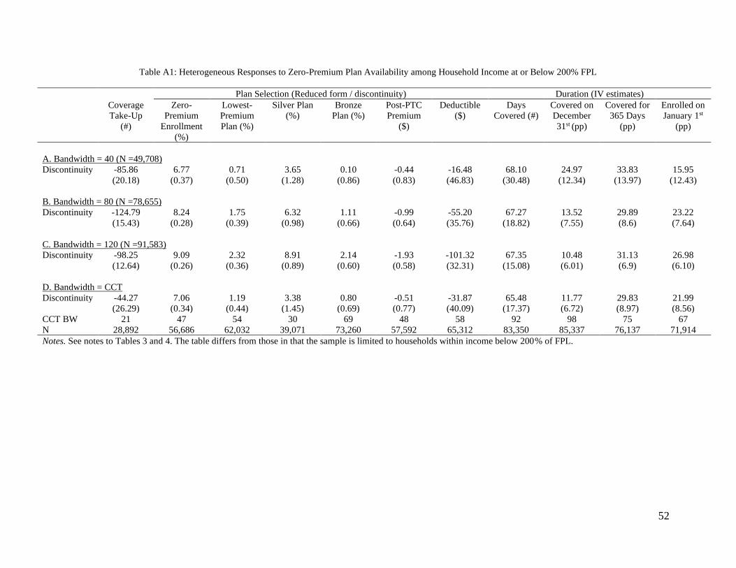
52

Table A1: Heterogeneous Responses to Zero-Premium Plan Availability among Household Income at or Below 200% FPL

Plan Selection (Reduced form / discontinuity) Duration (IV estimates)

Coverage

Take-Up

(#)

Zero-

Premium

Enrollment

(%)

Lowest-

Premium

Plan (%)

Silver Plan

(%)

Bronze

Plan (%)

Post-PTC

Premium

($)

Deductible

($)

Days

Covered (#)

Covered on

December

31st (pp)

Covered for

365 Days

(pp)

Enrolled on

January 1st

(pp)

A. Bandwidth = 40 (N =49,708)

Discontinuity -85.86 6.77 0.71 3.65 0.10 -0.44 -16.48 68.10 24.97 33.83 15.95

(20.18) (0.37) (0.50) (1.28) (0.86) (0.83) (46.83) (30.48) (12.34) (13.97) (12.43)

B. Bandwidth = 80 (N =78,655)

Discontinuity -124.79 8.24 1.75 6.32 1.11 -0.99 -55.20 67.27 13.52 29.89 23.22

(15.43) (0.28) (0.39) (0.98) (0.66) (0.64) (35.76) (18.82) (7.55) (8.6) (7.64)

C. Bandwidth = 120 (N =91,583)

Discontinuity -98.25 9.09 2.32 8.91 2.14 -1.93 -101.32 67.35 10.48 31.13 26.98

(12.64) (0.26) (0.36) (0.89) (0.60) (0.58) (32.31) (15.08) (6.01) (6.9) (6.10)

D. Bandwidth = CCT

Discontinuity -44.27 7.06 1.19 3.38 0.80 -0.51 -31.87 65.48 11.77 29.83 21.99

(26.29) (0.34) (0.44) (1.45) (0.69) (0.77) (40.09) (17.37) (6.72) (8.97) (8.56)

CCT BW 21 47 54 30 69 48 58 92 98 75 67

N 28,892 56,686 62,032 39,071 73,260 57,592 65,312 83,350 85,337 76,137 71,914

Notes. See notes to Tables 3 and 4. The table differs from those in that the sample is limited to households within income below 200% of FPL.

53

Table A2: Heterogeneous Responses to Zero-Premium Plan Availability among Household Income Above 200% FPL

Plan Selection (Reduced form / discontinuity) Duration (IV estimates)

Coverage

Take-Up

(#)

Zero-

Premium

Enrollment

(%)

Lowest-

Premium

Plan (%)

Silver Plan

(%)

Bronze

Plan (%)

Post-PTC

Premium

($)

Deductible

($)

Days

Covered (#)

Covered on

December

31st (pp)

Covered for

365 Days

(pp)

Enrolled on

January 1st

(pp)

A. Bandwidth = 40 (N =24,953)

Discontinuity -5.65 9.93 -0.74 -0.99 -1.33 1.42 51.03 -52.88 -20.34 -19.91 8.44

(11.79) (0.67) (0.91) (4.36) (1.41) (1.42) (52.37) (29.32) (12.2) (13.75) (10.68)

B. Bandwidth = 80 (N =52,922)

Discontinuity -24.06 10.69 0.49 1.11 -1.57 1.93 52.05 -24.97 -11.04 -9.66 8.10

(9.15) (0.51) (0.67) (3.15) (1.01) (1.02) (37.48) (19.28) (8.05) (9.11) (7.11)

C. Bandwidth = 120 (N =82,347)

Discontinuity -36.51 11.22 1.44 3.22 -2.09 2.16 43.04 -23.34 -5.11 -7.85 1.10

(7.75) (0.45) (0.57) (2.63) (0.85) (0.85) (31.3) (15.13) (6.31) (7.17) (5.6)

D. Bandwidth = CCT

Discontinuity 1.12 10.47 0.21 0.16 -2.55 2.20 38.87 -34.51 -13.39 -13.64 9.01

(12.6) (0.54) (0.71) (3.65) (0.77) (0.84) (32.67) (22.04) (8.64) (10.47) (8.19)

CCT BW 24 69 69 58 152 125 108 65 72 64 64

N 14,660 44,621 44,399 37,033 101,579 85,807 74,792 41,576 46,601 41,100 40,967

Notes. See notes to Tables 3 and 4. The table differs from those in that the sample is limited to households within income above 200% of FPL.

54

Table A3: Heterogeneous Responses to Zero-Premium Plan Availability among Newly Enrolled Households

Plan Selection (Reduced form / discontinuity) Duration (IV estimates)

Coverage

Take-Up

(#)

Zero-

Premium

Enrollment

(%)

Lowest-

Premium

Plan (%)

Silver Plan

(%)

Bronze

Plan (%)

Post-PTC

Premium

($)

Deductible

($)

Days

Covered (#)

Covered on

December

31st (pp)

Covered for

365 Days

(pp)

Enrolled on

January 1st

(pp)

A. Bandwidth = 40 (N =40,415)

Discontinuity -75.36 8.26 0.51 5.90 -0.39 -0.07 28.78 31.49 3.21 7.19 5.96

(20.95) (0.45) (0.6) (2.09) (0.98) (0.96) (52.16) (27.92) (10.98) (12.58) (12.59)

B. Bandwidth = 80 (N =70,429)

Discontinuity -124.26 8.99 0.85 8.95 0.12 -0.01 39.26 41.61 -0.64 12.74 17.80

(13.26) (0.34) (0.46) (1.55) (0.72) (0.71) (38.29) (18.85) (7.41) (8.49) (8.53)

C. Bandwidth = 120 (N =92,655)

Discontinuity -121.95 9.20 0.83 9.46 0.73 -0.71 0.70 47.17 -0.74 20.03 26.27

(10.37) (0.30) (0.40) (1.33) (0.62) (0.60) (32.4) (15.61) (6.14) (7.05) (7.10)

D. Bandwidth = CCT

Discontinuity -53.36 9.16 0.82 9.33 -0.29 0.24 43.24 50.06 2.09 23.46 30.69

(30.08) (0.31) (0.41) (1.40) (0.81) (0.80) (46.4) (15.13) (5.37) (6.75) (6.69)

CCT BW 24 108 108 104 61 60 52 130 168 134 140

N 25,482 86,932 86,760 85,112 57,127 56,063 49,986 97,007 112,199 98,963 101,416

Notes. See notes to Tables 3 and 4. The table differs from those in that the sample is limited to households without prior year coverage in the Colorado Marketplace.

55

Table A4: Heterogeneous Responses to Zero-Premium Plan Availability among Returning Households

Plan Selection (Reduced form / discontinuity) Duration (IV estimates)

Coverage

Take-Up

(#)

Zero-

Premium

Enrollment

(%)

Lowest-

Premium

Plan (%)

Silver Plan

(%)

Bronze

Plan (%)

Post-PTC

Premium

($)

Deductible

($)

Days

Covered (#)

Covered on

December

31st (pp)

Covered for

365 Days

(pp)

Enrolled on

January 1st

(pp)

A. Bandwidth = 40 (N =34,246)

Discontinuity -16.15 7.16 0.15 0.55 -1.03 1.03 54.99 3.11 18.50 16.23 9.23

(15.77) (0.48) (0.64) (2.69) (1.13) (1.11) (59.71) (32.77) (14.57) (15.1) (6.94)

B. Bandwidth = 80 (N =61,148)

Discontinuity -24.60 9.07 1.94 1.60 0.04 0.09 -18.35 20.84 16.41 13.80 3.70

(12.75) (0.36) (0.48) (1.95) (0.82) (0.81) (43.26) (18.73) (8.3) (8.61) (3.98)

C. Bandwidth = 120 (N =81,275)

Discontinuity -12.81 10.27 2.97 0.54 1.17 -1.08 -128.71 26.99 17.74 16.05 2.80

(10.26) (0.32) (0.42) (1.65) (0.7) (0.69) (37.04) (13.88) (6.15) (6.38) (2.95)

D. Bandwidth = CCT

Discontinuity -10.90 7.23 0.92 0.23 -0.72 0.80 46.48 28.76 18.49 17.28 2.76

(16.08) (0.47) (0.55) (1.56) (0.97) (0.95) (57.71) (11.73) (5.15) (5.43) (2.24)

CCT BW 29 42 57 141 55 56 43 156 158 154 185

N 25,504 35,976 46,657 89,630 45,415 45,584 36,449 94,901 95,761 94,421 103,996

Notes. See notes to Tables 3 and 4. The table differs from those in that the sample is limited to households with prior year coverage in the Colorado Marketplace.

56

Table A5: Robustness to Quadratic Form

Plan Selection (Reduced form / discontinuity) Duration (IV estimates)

Zero-

Premium

Enrollment

(%)

Lowest-

Premium

Plan (%)

Silver Plan

(%)

Bronze

Plan (%)

Post-PTC

Premium

($)

Deductible

($)

Days

Covered (#)

Covered on

December

31st (pp)

Covered for

365 Days

(pp)

Enrolled on

January 1st

(pp)

A. Bandwidth = 40 (N = 74,661)

Discontinuity 7.58 -0.01 -1.63 1.15 2.54 101.3 34.54 16.69 18.54 9.04

(0.46) (0.63) (1.09) (1.07) (2.43) (58.46) (32.33) (13.2) (14.98) (12.96)

B. Bandwidth = 80 (N = 131,577)

Discontinuity 7.5 0.19 -1.22 1.04 3.61 69.38 21.92 6.84 13.21 13.85

(0.34) (0.47) (0.80) (0.78) (1.78) (42.56) (23.45) (9.55) (10.86) (9.41)

C. Bandwidth = 120 (N = 173,930)

Discontinuity 8.31 0.77 -0.99 1.09 5.83 100.02 40.28 5.50 19.5 23.06

(0.29) (0.40) (0.67) (0.66) (1.50) (35.73) (17.72) (7.19) (8.21) (7.11)

D. Bandwidth = CCT (Quadratic)

Discontinuity 8.33 0.86 -0.54 1.04 5.85 98.26 47.77 6.39 26.72 31

(0.29) (0.39) (0.56) (0.63) (1.36) (36.05) (12.83) (4.72) (5.96) (4.83)

CCT BW 121 126 197 135 154 117 206 247 207 232

N 175,230 179,593 230,207 186,501 200,876 171,668 236,173 256,940 236,674 250,414

E. Bandwidth = CCT (Quadratic, covariate unadjusted), include covariates

Discontinuity 8.28 0.76 0.68 -0.38 0.18 -25.19 33.93 3.18 19.13 24.12

(0.29) (0.39) (0.54) (0.60) (1.18) (32.16) (12.80) (4.71) (5.92) (4.77)

CCT BW 121 126 197 135 154 117 206 247 207 232

N 175,230 179,593 230,207 186,501 200,876 171,668 236,173 256,940 236,674 250,414

F. Bandwidth = CCT (Quadratic, covariate adjusted), include covariates

Discontinuity 8.20 0.63 0.62 -0.50 0.31 -18.46 34.81 3.45 18.78 22.97

(0.30) (0.40) (0.56) (0.56) (1.14) (31.31) (12.38) (4.40) (5.99) (5.11)

CCT BW 116 117 175 163 170 126 219 284 203 205

N 170,812 170,962 215,946 207,339 212,250 178,735 243,707 268,059 234,200 235,308

Notes. All plan selection outcomes are estimated for households. Panels A-D are covariates unadjusted. We applied CCT bandwidths obtained without covariates

in panel D to panel E and added covariate adjustment. Finally, we used CCT-adjusted bandwidth in panel F. We present estimates with quadratic control for all

outcomes and IV estimates for all duration outcomes.