zero-shot recognition via semantic embeddings and ...xiaolonw/papers/cvpr2018_gcn_zeroshot.pdf ·...

Zero-shot Recognition via Semantic Embeddings and Knowledge Graphs

Xiaolong Wang∗ Yufei Ye∗ Abhinav GuptaThe Robotics Institute, Carnegie Mellon University

Abstract

We consider the problem of zero-shot recognition: learn-ing a visual classifier for a category with zero training ex-amples, just using the word embedding of the category andits relationship to other categories, which visual data areprovided. The key to dealing with the unfamiliar or novelcategory is to transfer knowledge obtained from familiarclasses to describe the unfamiliar class. In this paper, webuild upon the recently introduced Graph ConvolutionalNetwork (GCN) and propose an approach that uses bothsemantic embeddings and the categorical relationships topredict the classifiers. Given a learned knowledge graph(KG), our approach takes as input semantic embeddings foreach node (representing visual category). After a series ofgraph convolutions, we predict the visual classifier for eachcategory. During training, the visual classifiers for a fewcategories are given to learn the GCN parameters. At testtime, these filters are used to predict the visual classifiers ofunseen categories. We show that our approach is robust tonoise in the KG. More importantly, our approach providessignificant improvement in performance compared to the cur-rent state-of-the-art results (from 2 ∼ 3% on some metricsto whopping 20% on a few).

1. IntroductionConsider the animal category “okapi”. Even though we

might have never heard of this category or seen visual ex-amples in the past, we can still learn a good visual classi-fier based on the following description: ”zebra-striped fourlegged animal with a brown torso and a deer-like face” (Testyourself on figure 1). On the other hand, our current recogni-tion algorithms still operate in closed world conditions: thatis, they can only recognize the categories they are trainedwith. Adding a new category requires collecting thousandsof training examples and then retraining the classifiers. Totackle this problem, zero-shot learning is often used.

The key to dealing with the unfamiliar or novel categoryis to transfer knowledge obtained from familiar classes to de-scribe the unfamiliar classes (generalization). There are two

∗Indicates equal contribution.

Figure 1. Can you find “okapi” in these images? Okapi is ” zebra-striped four legged animal with a brown torso and a deer-likeface”. In this paper, we focus on the problem of zero-shot learningwhere visual classifiers are learned from semantic embeddings andrelationships to other categories.

paradigms of transferring knowledge. The first paradigmis to use implicit knowledge representations, i.e. semanticembeddings. In this approach, one learns a vector represen-tation of different categories using text data and then learnsa mapping between the vector representation to visual clas-sifier directly [33, 13]. However, these methods are limitedby the generalization power of the semantic models and themapping models themselves. It is also hard to learn semanticembeddings from structured information.

The alternative and less-explored paradigm for zero-shotlearning is to use explicit knowledge bases or knowledgegraphs. In this paradigm, one explicitly represents the knowl-edge as rules or relationships between objects. These rela-tionships can then be used to learn zero-shot classifiers fornew categories. The simplest example would be to learnvisual classifiers of compositional categories. Given clas-sifiers of primitive visual concepts as inputs, [32] appliesa simple composition rule to generate classifiers for newcomplex concepts. However, in the general form, the rela-tionships can be more complex than simple compositionality.An interesting question we want to explore is if we can usestructured information and complex relationships to learnvisual classifiers without seeing any examples.

In this paper, we propose to distill both the implicit knowl-edge representations (i.e. word embedding) and explicitrelationships (i.e. knowledge graph) for learning visual clas-sifiers of novel classes. We build a knowledge graph whereeach node corresponds to a semantic category. These nodesare linked via relationship edges. The input to each node ofthe graph is the vector representation (semantic embedding)of each category. We then use Graph Convolutional Network

1

(GCN) [22] to transfer information (message-passing) be-tween different categories. Specifically, we train a 6-layerdeep GCN that outputs the classifiers of different categories.

We focus on the task of image classification. We considerboth of the test settings: (a) final test classes being only zero-shot classes (without training classes at test time); (b) at testtime the labels can be either the seen or the unseen classes,namely “generalized zero-shot setting” [16, 6, 48]. Weshow surprisingly powerful results and huge improvementsover classical baselines such as DeVise [13] , ConSE [33],and current state-of-the-art [5]. For example, on standardImageNet with 2-hop setting, 43.7% of the images retrievedby [5] in top-10 are correct. Our approach retrieves 62.4%images correctly. That is a whopping 18.7% improvementover the current state-of-the-art. More interestingly, weshow that our approach scales amazingly well and givinga significant improvement as we increase the size of theknowledge graph even if the graph is noisy.

2. Related WorkWith recent success of recognition systems, the focus has

now shifted to scaling these systems in terms of categories.As more realistic and practical settings are considered, theneed for zero-shot recognition – training visual classifierswithout any examples – has increased. Specifically, the prob-lem of mapping text to visual classifiers is very interesting.

Early work on zero-shot learning used attributes [11,24, 19] to represent categories as vector indicating pres-ence/absence of attributes. This vector representation canthen be mapped to learn visual classifiers. Instead of usingmanually defined attribute-class relationships, Rohrbach etal. [39, 37] mined these associations from different internetsources. Akata et al. [1] used attributes as side-information tolearn a semantic embedding which helps in zero-shot recog-nition. Recently, there have been approaches such as [36]which trys to match Wikipedia text to images by modelingnoise in the text description.

With the advancement of deep learning, most recent ap-proaches can be mapped into two main research directions.The first approach is to use semantic embeddings (implicitrepresentations). The core idea is to represent each categorywith learned vector representations that can be mapped tovisual classifiers [46, 43, 13, 40, 25, 15, 14, 18, 23, 4, 5].Socher et al. [43] proposed training two different neural net-works for image and language in an unsupervised manner,and then learning a linear mapping between image repre-sentations and word embeddings. Motivated by this work,Frome et al. [13] proposed a system called DeViSE to train amapping from image to word embeddings using a ConvNetand a transformation layer. By using the predicted embed-ding to perform nearest neighbor search, DeViSE scales upthe zero-shot recognition to thousands of classes. Instead oftraining a ConvNet to predict the word embedding directly,

Norouzi et al. [33] proposed another system named ConSEwhich constructs the image embedding by combining anexisting image classification ConvNet and word embeddingmodel. Recently, Changpinyo et al [4] proposed an approachto align semantic and visual manifolds via use of ‘phantom’classes. They report state-of-the-art results on ImageNetdataset using this approach. One strong shortcoming ofthese approaches is they do not use any explicit relation-ships between classes but rather use semantic-embeddingsto represent relationships.

The second popular way to distill the knowledge is touse knowledge graph (explicit knowledge representations).Researchers have proposed several approaches on how touse knowledge graphs for object recognition [12, 42, 29, 34,38, 9, 8, 28, 47, 45]. For example, Salakhutdinov et al. [42]used WordNet to share the representations among differentobject classifiers so that objects with few training examplescan borrow statistical strength from related objects. On theother hand, the knowledge graph can also be used to modelthe mutual exclusion among different classes. Deng et al. [9]applied these exclusion rules as a constraint in the loss fortraining object classifiers (e.g. an object will not be a dogand a cat at the same time). They have also shown zero-shot applications by adding object-attribute relations intothe graph. In contrast to these methods of using graph asconstraints, our approach used the graph to directly generatenovel object classifiers [32, 10, 2].

In our work, we propose to distill information both viasemantic embeddings and knowledge graphs. Specifically,given a word embedding of an unseen category and theknowledge graph that encodes explicit relationships, ourapproach predicts the visual classifiers of unseen categories.To model the knowledge graph, our work builds upon therecently proposed Graph Convolutional Networks [22]. Itwas originally proposed as a method for semi-supervisedlearning in language processing. We extend it to our zero-short learning problem by changing the model architectureand training loss.

3. ApproachOur goal is to distill information from both implicit (word-

embeddings) and explicit (knowledge-graph) representationsfor zero-shot recognition. But what is the right way to extractinformation? We build upon the recent work on Graph Con-volutional Network (GCN) [22] to learn visual classifiers. Inthe following, we will first introduce how the GCN is appliedin natural language processing for classification tasks, andthen we will go into details about our approach: applyingthe GCN with a regression loss for zero-shot learning.

3.1. Preliminaries: Graph Convolutional Network

Graph Convolutional Network (GCN) was introducedin [22] to perform semi-supervised entity classification.

2

𝑥"

𝑥#

𝑥$𝑘 𝑐$

𝑤("

𝑤(#

𝑤($𝐷

𝑊$(𝑘×𝑐$)

Conv.

𝑊.(𝑐./$×𝐷)

Conv.⋯

𝑤"

𝑤#

Inputs: Word Embeddings 𝒳(𝑘 dimensions )

Outputs: Object classifiers 𝒲3(𝐷 dimensions )

Hidden states(𝑐$ dimensions)

Figure 2. An example of our Graph Convolutional Network. It takes word embeddings as inputs and outputs the object classifiers. Thesupervision comes from the ground-truth classifiers w2 and w3 highlighted by green. During testing, we input the same word embeddingsand obtain classifier for x1 as w1. This classifier will be multiplied with the image features to produce classification scores.

Given object entities, represented by word embeddings ortext features, the task is to perform classification. For ex-ample, entities such as “dog” and “cat” will be labeled as“mammal”; “chair” and “couch” will be labeled “furniture”.We also assume that there is a graph where nodes are entitiesand the edges represent relationships between entities.

Formally, given a dataset with n entities (X,Y ) ={(xi, yi)}ni=1 where xi represents the word embedding forentity i and yi ∈ {1, ..., C} represents its label. In semi-supervised setting, we know the ground-truth labels for thefirst m entities. Our goal is to infer yi for the remainingn − m entities, which do not have labels, using the wordembedding and the relationship graph. In the relationshipgraph, each node is an entity and two nodes are linked if theyhave a relationship in between.

We use a function F (·) to represent the Graph Convolu-tional Network. It takes all the entity word embeddings Xas inputs at one time and outputs the SoftMax classificationresults for all of them as F (X). For simplicity, we denotethe output for the ith entity as Fi(X), which is a C dimen-sion SoftMax probability vector. In training time, we applythe SoftMax loss on the first m entities, which have labels as

1

m

m∑i=1

Lsoftmax(Fi(X), yi). (1)

The weights of F (·) are trained via back-propagation withthis loss. During testing time, we use the learned weightsto obtain the labels for the n −m entities with Fi(X), i ∈{m+ 1, ..., n}.

Unlike standard convolutions that operate on local regionin an image, in GCN the convolutional operations computethe response at a node based on the neighboring nodes de-fined by the adjacency graph. Mathematically, the convo-lutional operations for each layer in the network F (·) isrepresented as

Z = AX ′W (2)

where A is a normalized version of the binary adjacency

matrix A of the graph, with n × n dimensions. X ′ is theinput n × k feature matrix from the former layer. W isthe weight matrix of the layer with dimension k × c, wherec is the output channel number. Therefore, the input to aconvolutional layer is n× k ,and the output is a n× c matrixZ. These convolution operations can be stacked one afteranother. A non-linear operation (ReLU) is also applied aftereach convolutional layer before the features are forwarded tothe next layer. For the final convolutional layer, the numberof output channels is the number of label classes (c = C).For more details, please refer to [22].

3.2. GCN for Zero-shot Learning

Our model builds upon the Graph Convolutional Network.However, instead of entity classification, we apply it to thezero-shot recognition with a regression loss. The input of ourframework is the set of categories and their correspondingsemantic-embedding vectors (represented by X = {xi}ni=1).For the output, we want to predict the visual classifier foreach input category (represented byW = {wi}ni=1).

Specifically, the visual classifier we want the GCN topredict is a logistic regression model on the fixed pre-trainedConvNet features. If the dimensionality of visual-featurevector is D, each classifier wi for category i is also a D-dimensional vector. Thus the output of each node in theGCN is D dimensions, instead of C dimensions. In thezero-shot setting, we assume that the first m categories inthe total n classes have enough visual examples to estimatetheir weight vectors. For the remaining n−m categories, wewant to estimate their corresponding weight vectors giventheir embedding vectors as inputs.

One way is to train a neural network (multi-layer percep-tron) which takes xi as an input and learns to predict wi asan output. The parameters of the network can be estimatedusing m training pairs. However, generally m is small (inthe order of a few hundreds) and therefore, we want to usethe explicit structure of the visual world or the relationshipsbetween categories to constrain the problem. We represent

3

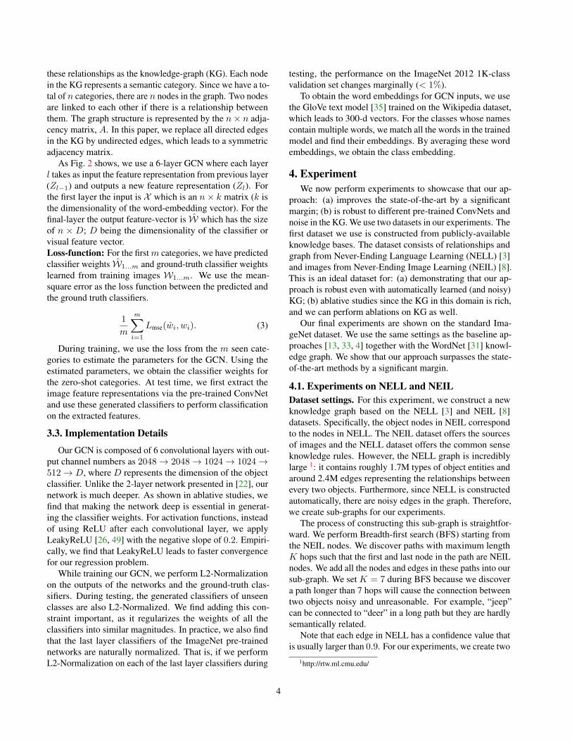
these relationships as the knowledge-graph (KG). Each nodein the KG represents a semantic category. Since we have a to-tal of n categories, there are n nodes in the graph. Two nodesare linked to each other if there is a relationship betweenthem. The graph structure is represented by the n× n adja-cency matrix, A. In this paper, we replace all directed edgesin the KG by undirected edges, which leads to a symmetricadjacency matrix.

As Fig. 2 shows, we use a 6-layer GCN where each layerl takes as input the feature representation from previous layer(Zl−1) and outputs a new feature representation (Zl). Forthe first layer the input is X which is an n× k matrix (k isthe dimensionality of the word-embedding vector). For thefinal-layer the output feature-vector is W which has the sizeof n × D; D being the dimensionality of the classifier orvisual feature vector.Loss-function: For the first m categories, we have predictedclassifier weights W1...m and ground-truth classifier weightslearned from training images W1...m. We use the mean-square error as the loss function between the predicted andthe ground truth classifiers.

1

m

m∑i=1

Lmse(wi, wi). (3)

During training, we use the loss from the m seen cate-gories to estimate the parameters for the GCN. Using theestimated parameters, we obtain the classifier weights forthe zero-shot categories. At test time, we first extract theimage feature representations via the pre-trained ConvNetand use these generated classifiers to perform classificationon the extracted features.

3.3. Implementation Details

Our GCN is composed of 6 convolutional layers with out-put channel numbers as 2048→ 2048→ 1024→ 1024→512→ D, where D represents the dimension of the objectclassifier. Unlike the 2-layer network presented in [22], ournetwork is much deeper. As shown in ablative studies, wefind that making the network deep is essential in generat-ing the classifier weights. For activation functions, insteadof using ReLU after each convolutional layer, we applyLeakyReLU [26, 49] with the negative slope of 0.2. Empiri-cally, we find that LeakyReLU leads to faster convergencefor our regression problem.

While training our GCN, we perform L2-Normalizationon the outputs of the networks and the ground-truth clas-sifiers. During testing, the generated classifiers of unseenclasses are also L2-Normalized. We find adding this con-straint important, as it regularizes the weights of all theclassifiers into similar magnitudes. In practice, we also findthat the last layer classifiers of the ImageNet pre-trainednetworks are naturally normalized. That is, if we performL2-Normalization on each of the last layer classifiers during

testing, the performance on the ImageNet 2012 1K-classvalidation set changes marginally (< 1%).

To obtain the word embeddings for GCN inputs, we usethe GloVe text model [35] trained on the Wikipedia dataset,which leads to 300-d vectors. For the classes whose namescontain multiple words, we match all the words in the trainedmodel and find their embeddings. By averaging these wordembeddings, we obtain the class embedding.

4. ExperimentWe now perform experiments to showcase that our ap-

proach: (a) improves the state-of-the-art by a significantmargin; (b) is robust to different pre-trained ConvNets andnoise in the KG. We use two datasets in our experiments. Thefirst dataset we use is constructed from publicly-availableknowledge bases. The dataset consists of relationships andgraph from Never-Ending Language Learning (NELL) [3]and images from Never-Ending Image Learning (NEIL) [8].This is an ideal dataset for: (a) demonstrating that our ap-proach is robust even with automatically learned (and noisy)KG; (b) ablative studies since the KG in this domain is rich,and we can perform ablations on KG as well.

Our final experiments are shown on the standard Ima-geNet dataset. We use the same settings as the baseline ap-proaches [13, 33, 4] together with the WordNet [31] knowl-edge graph. We show that our approach surpasses the state-of-the-art methods by a significant margin.

4.1. Experiments on NELL and NEILDataset settings. For this experiment, we construct a newknowledge graph based on the NELL [3] and NEIL [8]datasets. Specifically, the object nodes in NEIL correspondto the nodes in NELL. The NEIL dataset offers the sourcesof images and the NELL dataset offers the common senseknowledge rules. However, the NELL graph is incrediblylarge 1: it contains roughly 1.7M types of object entities andaround 2.4M edges representing the relationships betweenevery two objects. Furthermore, since NELL is constructedautomatically, there are noisy edges in the graph. Therefore,we create sub-graphs for our experiments.

The process of constructing this sub-graph is straightfor-ward. We perform Breadth-first search (BFS) starting fromthe NEIL nodes. We discover paths with maximum lengthK hops such that the first and last node in the path are NEILnodes. We add all the nodes and edges in these paths into oursub-graph. We set K = 7 during BFS because we discovera path longer than 7 hops will cause the connection betweentwo objects noisy and unreasonable. For example, “jeep”can be connected to “deer” in a long path but they are hardlysemantically related.

Note that each edge in NELL has a confidence value thatis usually larger than 0.9. For our experiments, we create two

1http://rtw.ml.cmu.edu/

4

All NEIL NodesDataset Nodes (Train/Test) EdgesHigh Value Edges 8819 431/88 40810All Edges 14612 616/88 96772

Table 1. Dataset Statistics: Two different sizes of knowledge graphsin our experiment.

different versions of sub-graphs. The first smaller version isa graph with high value edges (larger than 0.999), and thesecond one used all the edges regardless of their confidencevalues. The statistics of the two sub-graphs are summarizedin Table 1. For the larger sub-graph, we have 14K objectnodes. Among these nodes, 704 of them have correspondingimages in the NEIL database. We use 616 classes for trainingour GCN and leave 88 classes for testing. Note that these88 testing classes are randomly selected among the classesthat have no overlap with the 1000 classes in the standardImageNet classification dataset. The smaller knowledgegraph is around half the size of the larger one. We use thesame 88 testing classes in both settingsTraining details. For training the ConvNet on NEIL images,we use the 310K images associated with the 616 trainingclasses. The evaluation is performed on the randomly se-lected 12K images associated with the 88 testing classes,i.e. all images from the training classes are excluded duringtesting. We fine-tune the ImageNet pre-trained VGGM [7]network architecture with relatively small fc7 outputs (128-dimension). Thus the object classifier dimension in fc8 is128. For training our GCN, we use the ADAM [21] opti-mizer with learning rate 0.001 and weight decay 0.0005. Wetrain our GCN for 300 epochs for every experiment.Baseline method. We compare our method with one of thestate-of-the-art methods, ConSE [33], which shows slightlybetter performance than DeViSE [13] in ImageNet. As abrief introduction, ConSE first feedforwards the test imageinto a ConvNet that is trained only on the training classes.With the output probabilities, ConSE selects top T predic-tions {pi}Ti=1 and the word embeddings {xi}Ti=1 [30] ofthese classes. It then generates a new word embedding byweighted averaging the T embeddings with the probability1T

∑Ti=1 pixi. This new embedding is applied to perform

nearest neighbors in the word embeddings of the testingclasses. The top retrieved classes are selected as the finalresult. We enumerate different values of T for evaluations.Quantitative Results. We perform evaluations on the taskof 88 unseen categories classification. Our metric is basedon the percentage of correctly retrieved test data (out of top kretrievals) for a given zero-shot class. The results are shownin Table 2. We evaluate our method on two different sizesof knowledge graphs. We use “High Value Edges” to denotethe knowledge graph constructed based on high confidenceedges. “All Edges” represents the graph constructed with allthe edges. We denote the baseline [33] as “ConSE(T)” where

Hit@k (%)Test Set Model 1 2 5 10

High Value

ConSE(5) 6.6 9.6 13.6 19.4

Edges

ConSE(10) 7.0 9.8 14.2 20.1ConSE(431) 6.7 9.7 14.9 20.5Ours 9.1 16.8 23.2 47.9

All Edges

ConSE(5) 7.7 10.1 13.9 19.5ConSE(10) 7.7 10.4 14.7 20.5ConSE(616) 7.7 10.5 15.7 21.4Ours 10.8 18.4 33.7 49.0

Table 2. Top-k accuracy for different models in different settings.

Figure 3. We randomly drop 5% to 50% of the edges in the “AllEdges” graph and show the top-1, top-5 and top-10 accuracies.

we set T to be 5, 10 and the number of training classes.Our method outperforms the ConSE baseline by a large

margin. In the “All Edges” dataset, our method outperformsConSE 3.6% in top-1 accuracy. More impressively, the ac-curacy of our method is almost 2 times as that of ConSEin top-2 metric and even more than 2 times in top-5 andtop-10 accuracies. These results show that using knowl-edge graph with word embeddings in our method leads tomuch better result than the state-of-the-art results with wordembeddings only.From small to larger graph. In addition to improving per-formance in zero-shot recognition, our method obtains moreperformance gain as our graph size increases. As shown inTable 2, our method performs better by switching from thesmall to larger graph. Our approach has obtained 2 ∼ 3% im-provements in all the metrics. On the other hand, there is lit-tle to no improvements in ConSE performance. It also showsthat the KG does not need to be hand-crafted or cleaned. Ourapproach is able to robustly handle the errors in the graphstructure.Resilience to Missing Edges We explore how the perfor-mance of our model changes if we randomly drop 5% to50% of the edges in the “All Edges” graph. As Fig. 3 shows,by dropping from 5% to 10% of edges, the performance ofour model changes negligibly. This is mainly because the

5

Figure 4. We compute the minimum Euclidean distances betweenpredicted and training classifiers. The distances are plotted bysorting them from small to large.

knowledge graph can have redundant information with 14Knodes and 97K edges connecting them. This again impliesthat our model is robust to small noisy changes in the graph.As we start deleting more than 30% of the edges, the accura-cies drop drastically. This indicates that the performance ofour model is highly correlated to the size of the knowledgegraph.Random Graph? It is clear that our approach can handlenoise in the graph. But does any random graph work? Todemonstrate that the structure of the graph is still criticalwe also created some trivial graphs: (i) star model: wecreate a graph with one single root node and only have edgesconnecting object nodes to the root node; (ii) random graph:all nodes in the graph are randomly connected. Table 3shows the results. It is clear that all the numbers are close torandom guessing, which means a reasonable graph plays animportant role and a random graph can have negative effectson the model.

Hit@k (%)Test Set Trivial KG 1 2 5 10

All EdgesStar Model 1.1 1.6 4.8 9.7Random Graph 1.0 2.2 5.6 11.3

Table 3. Top-k accuracy on trivial knowledge graphs we create.

How important is the depth of GCN? We show that mak-ing the Graph Convolutional Network deep is critical in ourproblem. We show the performance of using different num-bers of layers for our model on the “All Edges” knowledgegraph shown in Table 4. For the 2-layer model we use 512hidden neurons, and the 4-layer model has output channelnumbers as 2048 → 1024 → 512 → 128. We show thatthe performance keeps increasing as we make the modeldeeper from 2-layer to 6-layer. The reason is that increasingthe times of convolutions is essentially increasing the timesof message passing between nodes in the graph. However,we do not observe much gain by adding more layers above

Hit@k (%)Test Set Model 1 2 5 10

All EdgesOurs (2-layer) 5.3 8.7 15.5 24.3Ours (4-layer) 8.2 13.5 27.1 41.8Ours (6-layer) 10.8 18.4 33.7 49.0

Table 4. Top-k accuracy with different depths of our model.

the 6-layer model. One potential reason might be that theoptimization becomes harder as the network goes deeper.Is our network just copying classifiers as outputs? Eventhough we show our method is better than ConSE baseline, isit possible that it learns to selectively copy the nearby classi-fiers? To show our method is not learning this trivial solution,we compute the Euclidean distance between our generatedclassifiers and the training classifiers. More specifically, fora generated classifier, we compare it with the classifiers fromthe training classes that are at most 3-hops away. We calcu-late the minimum distance between each generated classifierand its neighbors. We sort the distances for all 88 classi-fiers and plot Fig. 4. As for reference, the distance between“wooden spoon” and “spoon” classifiers in the training set is0.26 and the distance between “wooden spoon” and “opti-mus prime” is 0.78. We can see that our predicted classifiers

Figure 5. t-SNE visualizations for our word embeddings and GCNoutput visual classifiers in the “All Edges” dataset. The test classesare shown in red.

6

Hit@k (%)Test Set Model ConvNets 1 2 5 10 20

2-hops

ConSE [4] Inception-v1 8.3 12.9 21.8 30.9 41.7ConSE(us) Inception-v1 12.4 18.4 25.3 28.5 31.8SYNC [4] Inception-v1 10.5 17.7 28.6 40.1 52.0EXEM [5] Inception-v1 12.5 19.5 32.3 43.7 55.2Ours Inception-v1 18.5 31.3 50.1 62.4 72.0Ours ResNet-50 19.8 33.3 53.2 65.4 74.6

3-hops


All


(a) Top-k accuracy for different models when testing on only unseenclasses.

Hit@k (%)Test Set Model ConvNets 1 2 5 10 20

2-hops

DeViSE [13] AlexNet 0.8 2.7 7.9 14.2 22.7

(+1K)

ConSE [33] AlexNet 0.3 6.2 17.0 24.9 33.5ConSE(us) Inception-v1 0.2 7.8 18.1 22.8 26.4ConSE(us) ResNet-50 0.1 11.2 24.3 29.1 32.7Ours Inception-v1 7.9 18.6 39.4 53.8 65.3Ours ResNet-50 9.7 20.4 42.6 57.0 68.2

3-hops

DeViSE [13] AlexNet 0.5 1.4 3.4 5.9 9.7

(+1K)


All

DeViSE [13] AlexNet 0.3 0.8 1.9 3.2 5.3

(+1K)


(b) Top-k accuracy for different models when testing on both seen andunseen classes (a more practical and generalized setting).

Table 5. Results on ImageNet. We test our model on 2 different settings over 3 different datasets.

are quite different from its neighbors.Are the outputs only relying on the word embeddings?We perform t-SNE [27] visualizations to show that our out-put classifiers are not just derived from the word embeddings.We show the t-SNE [27] plots of both the word embeddingsand the classifiers of the seen and unseen classes in the “AllEdges” dataset. As Fig. 5 shows, we have very different clus-tering results between the word embeddings and the objectclassifiers, which indicates that our GCN is not just learninga direct projection from word embeddings to classifiers.

4.2. Experiments on WordNet and ImageNetWe now perform our experiments on a much larger-scale

ImageNet [41] dataset. We adopt the same train/test splitsettings as [13, 33]. More specifically, we report our resultson 3 different test datasets: “2-hops”, “3-hops” and thewhole “All” ImageNet set. These datasets are constructedaccording to how similar the classes are related to the classesin the ImageNet 2012 1K dataset. For example, “2-hops”dataset (around 1.5K classes) includes the classes from theImageNet 2011 21K set which are semantically very similarto the ImageNet 2012 1K classes. “3-hops” dataset (around7.8K classes) includes the classes that are within 3 hops ofthe ImageNet 2012 1K classes, and the “All” dataset includesall the labels in ImageNet 2011 21K. There are no commonlabels between the ImageNet 1K class and the classes inthese 3-dataset. It is also obvious to see that as the numberof class increases, the task becomes more challenging.

As for knowledge graph, we use the sub-graph of theWordNet [31], which includes around 30K object nodes.Note that all the classes in ImageNet are inside the WordNet.Training details. Note that to perform testing on 3 differ-ent test sets, we only need to train one set of ConvNet and

GCN. We use two different types of ConvNets as the basenetwork for computing visual features: Inception-v1 [44]and ResNet-50 [17]. Both networks are pre-trained usingthe ImageNet 2012 1K dataset and no fine-tuning is required.For Inception-v1, the output feature of the second to thelast layer has 1024 dimensions, which leads to D = 1024object classifiers in the last layer. For ResNet-50, we haveD = 2048. Except for the changes of output targets, othersettings of training GCN remain the same as those of the pre-vious experiments on NELL and NEIL. It is worthy to notethat our GCN model is robust to different sizes of outputs.The model shows consistently better results as the represen-tation (features) improves from Inception-v1 (68.7% top-1accuracy in ImageNet 1K val set) to ResNet-50 (75.3%).

We evaluate our method with the same metric as theprevious experiments: the percentage of hitting the ground-truth labels among the top k predictions. However, insteadof only testing with the unseen object classifiers, we includeboth training and the predicted classifiers during testing, assuggested by [13, 33]. Note that in these two settings ofexperiments, we still perform testing on the same set ofimages associated with unseen classes only.

Testing without considering the training labels. We firstperform experiments excluding the classifiers belonging tothe training classes during testing. We report our results inTable. 5a. We compare our results to the recent state-of-the-art methods SYNC [4] and EXEM [5]. We show experimentswith the same pre-trained ConvNets (Inception-v1) as [4, 5].Due to unavailability of their word embeddings for all thenodes in KG, we use a different set of word embeddings(GloVe) ,which is publicly available.

Therefore, we first investigate if the change of word-

7

Word Hit@k (%)Model Embedding 1 2 5 10 20[50] GloVe 7.8 11.5 17.2 21.2 25.6Ours GloVe 18.5 31.3 50.1 62.4 72.0[50] FastText 9.8 16.4 27.8 37.6 48.4Ours FastText 18.7 30.8 49.6 62.0 71.5[50] GoogleNews 13.0 20.6 33.5 44.1 55.2Ours GoogleNews 18.3 31.6 51.1 63.4 73.0

Table 6. Results with different word embeddings on ImageNet (2hops), corresponding to the experiments in Table 5a.

embedding is crucial. We show this via the ConSE baseline.Our re-implementation of ConSE, shown as “ConSE(us)”in the table, uses the GloVe whereas the ConSE methodimplemented in [4, 5] uses their own word embedding. Wesee that both approaches have similar performance. Ours isslightly better in top-1 accuracy while the one in [4, 5] isbetter in top-20 accuracy. Thus, with respect to zero-shotlearning, both word-embeddings seem equally powerful.

We then compare our results with SYNC [4] andEXEM [5]. With the same pre-trained ConvNet Inception-v1, our method outperforms almost all the other methods onall the datasets and metrics. On the “2-hops” dataset, our ap-proach outperforms all methods with a large margin: around6% on top-1 accuracy and 17% on top-5 accuracy. On the“3-hops” dataset, our approach is consistently better thanEXEM [5] around 2 ∼ 3% from top-5 to top-20 metrics.

By replacing the Inception-v1 with the ResNet-50, weobtain another performance boost in all metrics. For thetop-5 metric, our final model outperforms the state-of-the-artmethod EXEM [5] by a whooping 20.9% in the “2-hops”dataset, 3.5% in the “3-hops” dataset and 1% in the “All”dataset. Note that the gain is diminishing because the taskincreases in difficulty as the number of unseen classes in-creases.Sensitivity to word embeddings. Is our method sensitiveto word embeddings? What will happen if we use differentword embeddings as inputs? We investigate 3 different wordembeddings including GloVe [35] (which is used in the otherexperiments in the paper), FastText [20] and word2vec [30]trained with GoogleNews. As for comparisons, we havealso implemented the method in [50] which trains a directmapping from word embeddings to visual features withoutknowledge graphs. We use the Inception-v1 ConvNet to ex-tract visual features. We show the results on ImageNet (withthe 2-hops setting same as Table 5a). We can see that [50]highly relies on the quality of the word embeddings (top-5results range from 17.2% to 33.5%). On the other hand, ourtop-5 results are stably around 50% and are much higherthan [50]. With the GloVe word embeddings, our approachhas a relative improvement of almost 200% over [50].This again shows graph convolutions with knowledge graphsplay a significant role in improving zero-shot recognition.

Test Image Test ImageConSE (10) Ours ConSE (10) Oursrobin (train)bulbul (train)linnet (train)erolia alpina (train)egretta albus (train)

nightingale (test)thrush (test) robin (train)bulbul (train) finch (test)

panthera tigris(train) tiger cat (train) felis onca (train) leopard (train) tiger shark (train)

tigress (test) bengal tiger (test) panthera tigris (train) tiger cub (test) tiger cat (train)

croquet ball (train) golf ball (train) tennis ball (train) ball (test) soccer ball (train)

croquet ball (train) croquet equip (test) ball (test) plunger (train) hand tool (test)

rock beauty (train) ringlet (train) flagpole (train) large slipper (test) yellow slipper (train)

butterfly fish (test) rock beauty (train) damselfish (test) atoll (test) barrier reef (test)

teapot (train) bell (train) horn (train) coffeepot(train) mouth harp (train)

brass (test) french horn (train) trombone (train) horn (train) coffeepot (train)

tractor (train) reaper (train) thresher (train) trailer truck (train) motortruck (test)

tracked vehicle (test) tractor (train) propelled vehicle (test) reaper (train) forklift (train)

Figure 6. Visualization of top 5 prediction results for 3 differentimages. The correct prediction results are highlighted by red boldcharacters. The unseen classes or zero-shot classes are marked witha red “test” in the bracket. Previously seen classes have a plain“train” in the bracket.

Testing with the training classifiers. Following the sug-gestions in [13, 33], a more practical setting for zero-shotrecognition is to include both seen and unseen category clas-sifiers during testing. We test our method in this generalizedsetting. Since there are very few baselines available forthis setting of experiment, we can only compare the resultswith ConSE and DeViSE. We have also re-implemented theConSE baselines with both Inception-v1 and ResNet-50 pre-trained networks. As Table 5b shows our method almostdoubles the performance compared to the baselines on ev-ery metric and all 3-datasets. Moreover, we can still seethe boost in of performance by switching the pre-trainedInception-v1 network to ResNet-50.Visualizations. We finally perform visualizations using ourmodel and the baseline model: ConSE with T = 10 in Fig.6 (Top-5 prediction results). We can see that our methodsignificantly outperforms ConSE(10) in these examples. Al-though ConSE(10) still gives reasonable classification resultsin most cases, the output labels are biased to be within thetraining labels. On the other hand, our method outputs theunseen classes as well.

5. ConclusionWe have presented an approach for zero-shot recogni-

tion using the semantic embeddings of a category and theknowledge graph that encodes the relationship of the novelcategory to familiar categories. Our work also shows thata knowledge graph provides supervision to learn meaning-ful classifiers on top of semantic embeddings. Our resultsindicate a significant improvement over current state-of-the-art. As future work, we plan to explore how we can userelationship types more explicitly in this framework.

8

References[1] Z. Akata, F. Perronnin, Z. Harchaoui, and C. Schmid. Label

embedding for attribute-based classification. In CVPR, 2013.2

[2] J. L. Ba, K. Swersky, S. Fidler, and R. Salakhutdinov. Predict-ing Deep Zero-Shot Convolutional Neural Networks usingTextual Descriptions. In ICCV, 2015. 2

[3] A. Carlson, J. Betteridge, B. Kisiel, B. Settles, E. R. H. Jr.,and T. M. Mitchell. Toward an architecture for never-endinglanguage learning. In AAAI, 2010. 4

[4] S. Changpinyo, W.-L. Chao, B. Gong, and F. Sha. SynthesizedClassifiers for Zero-Shot Learning. In CVPR, 2016. 2, 4, 7, 8

[5] S. Changpinyo, W.-L. Chao, and F. Sha. Predicting VisualExemplars of Unseen Classes for Zero-Shot Learning. InICCV, 2017. 2, 7, 8

[6] W.-L. Chao, S. Changpinyo, B. Gong, and F. Sha. An Empiri-cal Study and Analysis of Generalized Zero-Shot Learningfor Object Recognition in the Wild. In ECCV, 2016. 2

[7] K. Chatfield, K. Simonyan, A. Vedaldi, and A. Zisserman.Return of the devil in the details: Delving deep into convolu-tional nets. In BMVC, 2014. 5

[8] X. Chen, A. Shrivastava, and A. Gupta. Neil: Extractingvisual knowledge from web data. ICCV, 2013. 2, 4

[9] J. Deng, N. Ding, Y. Jia, A. Frome, K. Murphy, S. Bengio,Y. Li, H. Neven, and H. Adam. Large-Scale Object Classifi-cation Using Label Relation Graphs. In ECCV, 2014. 2

[10] M. Elhoseiny, B. Saleh, and A. Elgammal. Write a Classifier:Zero-Shot Learning Using Purely Textual Descriptions. InICCV, 2013. 2

[11] A. Farhadi, I. Endres, D. Hoiem, and D. Forsyth. Describingobjects by their attributes. In CVPR, 2009. 2

[12] R. Fergus, H. Bernal, Y. Weiss, and A. Torralba. SemanticLabel Sharing for Learning with Many Categories. In ECCV,2010. 2

[13] A. Frome, G. Corrado, J. Shlens, S. Bengio, J. Dean, andT. Mikolov. Devise: A deep visual-semantic embeddingmodel. In NIPS, 2013. 1, 2, 4, 5, 7, 8

[14] Y. Fu and L. Sigal. Semi-supervised Vocabulary-informedLearning. In CVPR, 2016. 2

[15] Z. Fu, T. Xiang, E. Kodirov, and S. Gong. Zero-Shot ObjectRecognition by Semantic Manifold Distance. In CVPR, 2015.2

[16] B. Hariharan and R. Girshick. Low-shot Visual Recognitionby Shrinking and Hallucinating Features. In CoRR, 2017. 2

[17] K. He, X. Zhang, S. Ren, and J. Sun. Deep residual learningfor image recognition. In CVPR, 2016. 7

[18] C. Huang, C. C. Loy, and X. Tang. Local similarity-awaredeep feature embedding. In NIPS, 2016. 2

[19] D. Jayaraman and K. Grauman. Zero-shot recognition withunreliable attributes. In NIPS, pages 3464–3472, 2014. 2

[20] A. Joulin, E. Grave, P. Bojanowski, M. Douze, H. Jegou,and T. Mikolov. Fasttext.zip: Compressing text classificationmodels. arXiv preprint arXiv:1612.03651, 2016. 8

[21] D. Kingma and J. Ba. Adam: A method for stochastic opti-mization. CoRR, abs/1412.6980, 2014. 5

[22] T. N. Kipf and M. Welling. Semi-supervised classificationwith graph convolutional networks. ICLR, 2017. 2, 3, 4

[23] E. Kodirov, T. Xiang, and S. Gong. Semantic Autoencoderfor Zero-Shot Learning. In CVPR, 2017. 2

[24] C. H. Lampert, H. Nickisch, and S. Harmeling. Learningto detect unseen object classes by between-class attributetransfer. In CVPR, 2009. 2

[25] C. H. Lampert, H. Nickisch, and S. Harmeling. Attribute-Based Classification for Zero-Shot Visual Object Categoriza-tion. In TPAMI, 2014. 2

[26] A. L. Maas, A. Y. Hannun, and A. Y. Ng. Rectifier nonlineari-ties improve neural network acoustic models. In ICML, 2013.4

[27] L. v. d. Maaten and G. Hinton. Visualizing data using t-sne.Journal of Machine Learning Research, 9(Nov):2579–2605,2008. 7

[28] K. Marino, R. Salakhutdinov, and A. Gupta. The More YouKnow: Using Knowledge Graphs for Image Classification. InCVPR, 2017. 2

[29] T. Mensink, J. Verbeek, F. Perronnin, and G. Csurka. MetricLearning for Large Scale Image Classification: Generalizingto New Classes at Near-Zero Cost. In ECCV, 2012. 2

[30] T. Mikolov, K. Chen, G. Corrado, and J. Dean. Efficientestimation of word representations in vector space. ICLR,2013. 5, 8

[31] G. A. Miller. Wordnet: a lexical database for english. Com-munications of the ACM, 38(11):39–41, 1995. 4, 7

[32] I. Misra, A. Gupta, and M. Hebert. From Red Wine to RedTomato: Composition with Context. In CVPR, 2017. 1, 2

[33] M. Norouzi, T. Mikolov, S. Bengio, Y. Singer, J. Shlens,A. Frome, G. S. Corrado, and J. Dean. Zero-shot learning byconvex combination of semantic embeddings. In ICLR, 2014.1, 2, 4, 5, 7, 8

[34] M. Palatucci, D. Pomerleau, G. E. Hinton, and T. M. Mitchell.Zero-shot Learning with Semantic Output Codes. In NIPS,2009. 2

[35] J. Pennington, R. Socher, and C. D. Manning. Glove: Globalvectors for word representation. In EMNLP, pages 1532–1543, 2014. 4, 8

[36] R. Qiao, L. Liu, C. Shen, and A. van den Hengel. Less ismore: zero-shot learning from online textual documents withnoise suppression. In CVPR, 2016. 2

[37] M. Rohrbach, S. Ebert, and B. Schiele. Transfer learning in atransductive setting. In NIPS, 2013. 2

[38] M. Rohrbach, M. Stark, and B. Schiele. Evaluating Knowl-edge Transfer and Zero-Shot Learning in a Large-Scale Set-ting. In CVPR, 2011. 2

[39] M. Rohrbach, M. Stark, G. Szarvas, I. Gurevych, andB. Schiele. What helps where - and why? semantic relat-edness for knowledge transfer. In CVPR, 2010. 2

[40] B. Romera-Paredes and P. H. S. Torr. An embarrassinglysimple approach to zero-shot learning. In ICML, 2015. 2

[41] O. Russakovsky, J. Deng, H. Su, J. Krause, S. Satheesh,S. Ma, Z. Huang, A. Karpathy, A. Khosla, M. Bernstein,et al. Imagenet large scale visual recognition challenge. IJCV,115(3):211–252, 2015. 7

9

[42] R. Salakhutdinov, A. Torralba, and J. Tenenbaum. Learningto Share Visual Appearance for Multiclass Object Detection.In CVPR, 2011. 2

[43] R. Socher, M. Ganjoo, C. D. Manning, and A. Y. Ng. Zero-Shot Learning Through Cross-Modal Transfer. In ICLR, 2013.2

[44] C. Szegedy, W. Liu, Y. Jia, P. Sermanet, S. Reed, D. Anguelov,D. Erhan, V. Vanhoucke, and A. Rabinovich. Going Deeperwith Convolutions. In CVPR, 2015. 7

[45] P. Wang, Q. Wu, C. Shen, A. van den Hengel, and A. Dick.FVQA: Fact-based Visual Question Answering. In CoRR,2016. 2

[46] J. Weston, S. Bengio, and N. Usunier. Large Scale ImageAnnotation: Learning to Rank with Joint Word-Image Em-beddings. In ECML, 2010. 2

[47] Q. Wu, P. Wang, C. Shen, A. Dick, and A. van den Hengel.Ask me anything: Free-form visual question answering basedon knowledge from external sources. In CVPR, 2016. 2

[48] Y. Xian, B. Schiele, and Z. Akata. Zero-Shot Learning - TheGood, the Bad and the Ugly. In CVPR, 2017. 2

[49] B. Xu, N. Wang, T. Chen, and M. Li. Empirical evalua-tion of rectified activations in convolutional network. CoRR,abs/1505.00853, 2015. 4

[50] L. Zhang, T. Xiang, and S. Gong. Learning a deep embeddingmodel for zero-shot learning. In CVPR, 2017. 8

10

zero-shot recognition via semantic embeddings and ...xiaolonw/papers/cvpr2018_gcn_zeroshot.pdf ·...

Documents