zhangxi lin isqs 7339 texas tech university review - decision trees

ZHANGXI LINISQS 7339

TEXAS TECH UNIVERSITY

Review - Decision Trees

Outline

ISQS 7342-001, Business Analytics

2

Basic decision tree modelingDetermining the best split Determining when to stop splitting

Basic Decision Tree Modeling

Classification: Definition


4

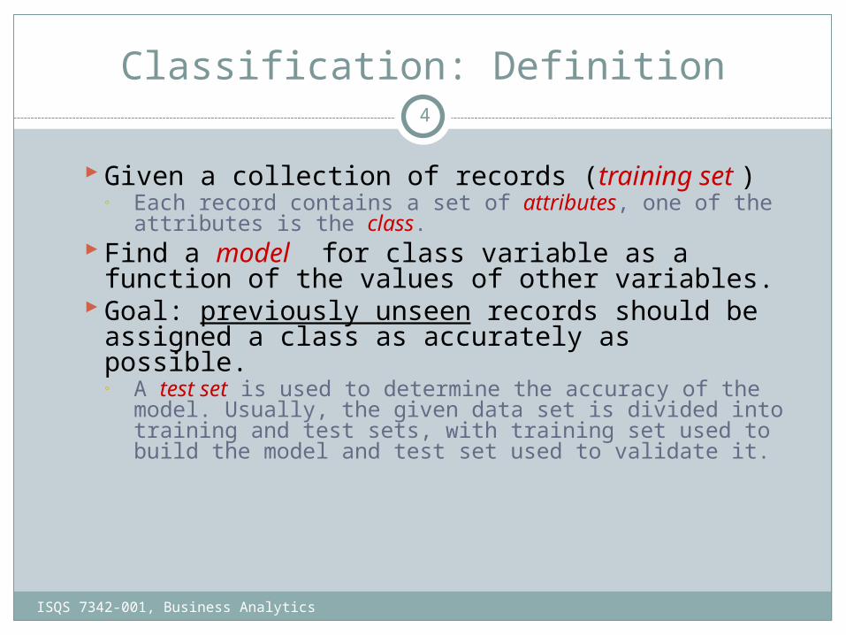
Given a collection of records (training set )◦ Each record contains a set of attributes, one of the

attributes is the class. Find a model for class variable as a function

of the values of other variables. Goal: previously unseen records should be

assigned a class as accurately as possible.◦ A test set is used to determine the accuracy of the

model. Usually, the given data set is divided into training and test sets, with training set used to build the model and test set used to validate it.

Decision Tree Based Classification


5

Advantages: Inexpensive to construct Extremely fast at classifying unknown records Easy to interpret for small-sized trees Accuracy is comparable to other classification

techniques for many simple data sets

Decision Tree Induction


6

Many Algorithms: Hunt’s Algorithm (one of the earliest) CHAID (Chi-square Automatic Interaction Detection) CRT (Classification and Regression Trees) ID3, C4.5 SLIQ,SPRINT

General Structure of Hunt’s Algorithm


7

Let Dt be the set of training records that reach a node t

General Procedure: If Dt contains records that

belong the same class yt, then t is a leaf node labeled as yt

If Dt is an empty set, then t is a leaf node labeled by the default class, yd

If Dt contains records that belong to more than one class, use an attribute test to split the data into smaller subsets. Recursively apply the procedure to each subset.

Tid Refund Marital Status

Taxable Income Cheat

1 Yes Single 125K No

2 No Married 100K No

3 No Single 70K No

4 Yes Married 120K No

5 No Divorced 95K Yes

6 No Married 60K No

7 Yes Divorced 220K No

8 No Single 85K Yes

9 No Married 75K No

10 No Single 90K Yes 10

Dt

?

Hunt’s Algorithm


8Don’t Cheat

Refund

Don’t Cheat

Don’t Cheat

Yes No

Refund

Don’t Cheat

Yes No

MaritalStatus

Don’t Cheat

Cheat

Single,Divorced

Married

TaxableIncome

Don’t Cheat

< 80K >= 80K

Refund

Don’t Cheat

Yes No

MaritalStatus

Don’t Cheat

Cheat

Single,Divorced

Married

Tree Induction


9

Greedy strategy. Split the records based on a variable test that

optimizes certain criterion.

Issues Determine how to split the records

How to specify the attribute test condition? How to determine the best split?

Determine when to stop splitting

How to Specify Test Condition?


10

Depends on variable types Nominal Ordinal Continuous

Depends on number of ways to split 2-way split Multi-way split

Splitting Based on Ordinal Variables


11

Multi-way split: Use as many partitions as distinct values.

Binary split: Divides values into two subsets. Need to find optimal partitioning.

What about this split?

SizeSmall

Medium

Large

Size{Medium,

Large} {Small}

Size{Small,

Medium} {Large}OR

Size{Small, Large} {Medium}

Splitting Based on Continuous Attributes


12

Different ways of handling Discretization to form an ordinal categorical attribute

Static – discretize once at the beginning Dynamic – ranges can be found by equal interval

bucketing, equal frequency bucketing(percentiles), or clustering.

Binary Decision: (A < v) or (A v) consider all possible splits and finds the best cut can be more compute intensive

Splitting Based on Continuous Attributes


13

TaxableIncome> 80K?

Yes No

TaxableIncome?

(i) Binary split (ii) Multi-way split

< 10K

[10K,25K) [25K,50K) [50K,80K)

> 80K

Determining the best split

Tree Induction


15

Greedy strategy. Split the records based on an variable test that





How to determine the Best Split


16

OwnCar?

C0: 6C1: 4

C0: 4C1: 6

C0: 1C1: 3

C0: 8C1: 0

C0: 1C1: 7

CarType?

C0: 1C1: 0

C0: 1C1: 0

C0: 0C1: 1

StudentID?

...

Yes No Family

Sports

Luxury c1c10

c20

C0: 0C1: 1

...

c11

Before Splitting: 10 records of class 0,10 records of class 1

Which test condition is the best?

How to determine the Best Split


17

C0: 5C1: 5

Greedy approach: Nodes with homogeneous class distribution are

preferred

Need a measure of node impurity:

C0: 9C1: 1

Non-homogeneous,

High degree of impurity

Homogeneous,

Low degree of impurity

Measures of Node Impurity


18

Gini Index

Entropy

Misclassification error

Measure of Impurity: GINI


19

Gini Index for a given node t :

(NOTE: p( j | t) is the relative frequency of class j at node t).

Maximum (1 - 1/nc) when records are equally distributed among all classes, implying least interesting information

Minimum (0.0) when all records belong to one class, implying most interesting information

j

tjptGINI 2)]|([1)(

C1 0C2 6

Gini=0.000

C1 2C2 4

Gini=0.444

C1 3C2 3

Gini=0.500

C1 1C2 5

Gini=0.278

Examples for computing GINI


20

C1 0 C2 6

C1 2 C2 4

C1 1 C2 5

P(C1) = 0/6 = 0 P(C2) = 6/6 = 1

Gini = 1 – P(C1)2 – P(C2)2 = 1 – 0 – 1 = 0

j

tjptGINI 2)]|([1)(

P(C1) = 1/6 P(C2) = 5/6

Gini = 1 – (1/6)2 – (5/6)2 = 0.278

P(C1) = 2/6 P(C2) = 4/6

Gini = 1 – (2/6)2 – (4/6)2 = 0.444

Splitting Based on GINI

Used in CART, SLIQ, SPRINT.When a node p is split into k partitions

(children), the quality of split is computed as,

where, ni = number of records at child i,

n = number of records at node p.

ISQS 7342-001, Business Analytics 21

k

i

isplit iGINI

n

nGINI

1

)(

Binary Variables: Computing GINI Index


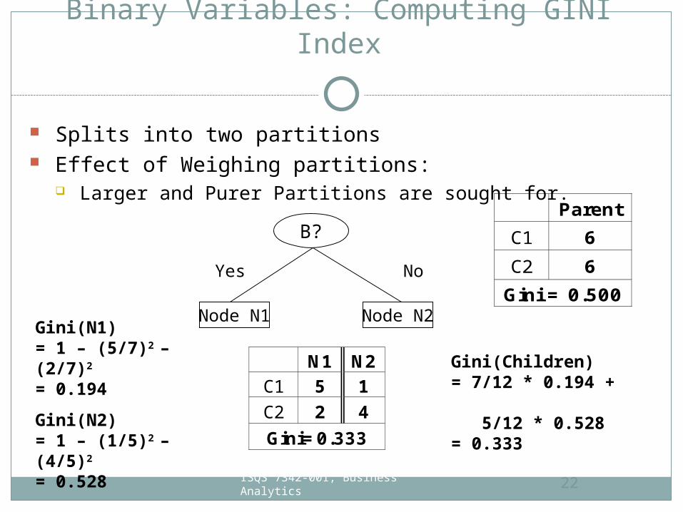
Splits into two partitions Effect of Weighing partitions:

Larger and Purer Partitions are sought for.

B?

Yes No

Node N1 Node N2

Parent

C1 6

C2 6

Gini = 0.500

N1 N2 C1 5 1

C2 2 4

Gini=0.333

Gini(N1) = 1 – (5/7)2 – (2/7)2 = 0.194

Gini(N2) = 1 – (1/5)2 – (4/5)2 = 0.528

Gini(Children) = 7/12 * 0.194 + 5/12 * 0.528= 0.333

Categorical Attributes: Computing Gini Index


23

For each distinct value, gather counts for each class in the dataset

Use the count matrix to make decisions

CarType{Sports,Luxury}

{Family}

C1 3 1

C2 2 4

Gini 0.400

CarType

{Sports}{Family,Luxury}

C1 2 2

C2 1 5

Gini 0.419

CarType

Family Sports Luxury

C1 1 2 1

C2 4 1 1

Gini 0.393

Multi-way split Two-way split (find best partition of values)

Continuous Variables: Computing Gini Index

Use Binary Decisions based on one value

Several Choices for the splitting value Number of possible splitting values

= Number of distinct values Each splitting value has a count

matrix associated with it Class counts in each of the

partitions, A < v and A v Simple method to choose best v

For each v, scan the database to gather count matrix and compute its Gini index

Computationally Inefficient! Repetition of work.

TaxableIncome> 80K?

Yes No


Continuous Variables: Computing Gini Index...


25

For efficient computation: for each attribute,◦ Sort the attribute on values◦ Linearly scan these values, each time updating the

count matrix and computing Gini index◦ Choose the split position that has the least Gini index

Cheat No No No Yes Yes Yes No No No No

Taxable Income

60 70 75 85 90 95 100 120 125 220

55 65 72 80 87 92 97 110 122 172 230

<= > <= > <= > <= > <= > <= > <= > <= > <= > <= > <= >

Yes 0 3 0 3 0 3 0 3 1 2 2 1 3 0 3 0 3 0 3 0 3 0

No 0 7 1 6 2 5 3 4 3 4 3 4 3 4 4 3 5 2 6 1 7 0

Gini 0.420 0.400 0.375 0.343 0.417 0.400 0.300 0.343 0.375 0.400 0.420

Split Positions

Sorted Values

Alternative Splitting Criteria based on INFO

Entropy at a given node t:

(NOTE: p( j | t) is the relative frequency of class j at node t).

Measures homogeneity of a node. Maximum (log nc) when records are equally

distributed among all classes implying least information

Minimum (0.0) when all records belong to one class, implying most information

Entropy based computations are similar to the GINI index computations

j

tjptjptEntropy )|(log)|()(2


Examples for computing Entropy


27

C1 0 C2 6

C1 2 C2 4

C1 1 C2 5

P(C1) = 0/6 = 0 P(C2) = 6/6 = 1

Entropy = – 0 log 0 – 1 log 1 = – 0 – 0 = 0

P(C1) = 1/6 P(C2) = 5/6

Entropy = – (1/6) log2 (1/6) – (5/6) log2 (1/6) = 0.65

P(C1) = 2/6 P(C2) = 4/6

Entropy = – (2/6) log2 (2/6) – (4/6) log2 (4/6) = 0.92

j

tjptjptEntropy )|(log)|()(2

Splitting Based on INFO...Information Gain:

Parent Node, p is split into k partitions;ni is number of records in partition i

Measures Reduction in Entropy achieved because of the split. Choose the split that achieves most reduction (maximizes GAIN)

Used in ID3 and C4.5 Disadvantage: Tends to prefer splits that result in

large number of partitions, each being small but pure.


k

i

isplit iEntropy

n

npEntropyGAIN

1

)()(

Splitting Based on INFO...Gain Ratio:

Parent Node, p is split into k partitionsni is the number of records in partition i

Adjusts Information Gain by the entropy of the partitioning (SplitINFO). Higher entropy partitioning (large number of small partitions) is penalized!

Used in C4.5 Designed to overcome the disadvantage of

Information GainISQS 7342-001, Business Analytics 29

SplitINFO

GAINGainRATIO Split

split

k

i

ii

nn

nn

SplitINFO1

log

Splitting Criteria based on Classification Error


30

Classification error at a node t :

Measures misclassification error made by a node. Maximum (1 - 1/nc) when records are equally distributed

among all classes, implying least interesting information Minimum (0.0) when all records belong to one class, implying

most interesting information

)|(max1)( tiPtErrori

Examples for Computing Error


31

C1 0 C2 6

C1 2 C2 4

C1 1 C2 5

P(C1) = 0/6 = 0 P(C2) = 6/6 = 1

Error = 1 – max (0, 1) = 1 – 1 = 0

P(C1) = 1/6 P(C2) = 5/6

Error = 1 – max (1/6, 5/6) = 1 – 5/6 = 1/6

P(C1) = 2/6 P(C2) = 4/6

Error = 1 – max (2/6, 4/6) = 1 – 4/6 = 1/3

)|(max1)( tiPtErrori

Comparison among Splitting Criteria


32For a 2-class problem:

Misclassification Error vs Gini


33

A?

Yes No

Node N1 Node N2

Parent

C1 7

C2 3

Gini = 0.42

N1 N2 C1 3 4

C2 0 3

Gini=0.361

Gini(N1) = 1 – (3/3)2 – (0/3)2 = 0

Gini(N2) = 1 – (4/7)2 – (3/7)2 = 0.489

Gini(Children) = 3/10 * 0 + 7/10 * 0.489= 0.342

Gini improves !!

Determining when to stop splitting

Tree Induction


35

Greedy strategy. Split the records based on an attribute test that





Stopping Criteria for Tree Induction


36

Stop expanding a node when all the records belong to the same class

Stop expanding a node when all the records have similar attribute values

Early termination

Issues in Classification


37

Underfitting and Overfitting

Missing Values

Costs of Classification

Underfitting and Overfitting (Example)


38

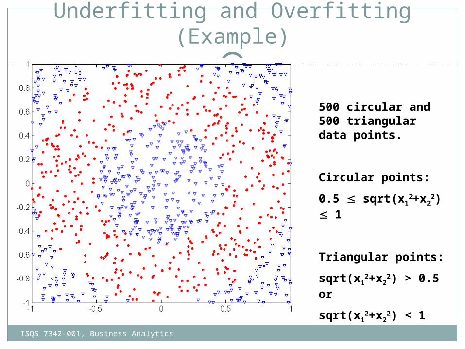
500 circular and 500 triangular data points.

Circular points:

0.5 sqrt(x12+x2

2) 1

Triangular points:

sqrt(x12+x2

2) > 0.5 or

sqrt(x12+x2

2) < 1

Underfitting and Overfitting


39

Overfitting

Underfitting: when model is too simple, both training and test errors are large

Overfitting


40

Training Set Test Set

Better Fitting


41

Training Set Test Set

How to Address Overfitting


42Pre-Pruning (Early Stopping Rule) Stop the algorithm before it becomes a fully-grown tree Typical stopping conditions for a node:

Stop if all instances belong to the same class Stop if all the attribute values are the same

More restrictive conditions: Stop if number of instances is less than some user-

specified threshold Stop if class distribution of instances are independent of

the available features (e.g., using 2 test) Stop if expanding the current node does not improve

impurity measures (e.g., Gini or information gain).

Data Splitting


43

How to Address Overfitting…


44

Post-pruning Grow decision tree to its entirety Trim the nodes of the decision tree in a bottom-up

fashion If generalization error improves after trimming,

replace sub-tree by a leaf node. Class label of leaf node is determined from majority

class of instances in the sub-tree Can use MDL for post-pruning

Example of Post-Pruning


45

A?

A1

A2 A3

A4

Class = Yes 20

Class = No 10

Error = 10/30

Training Error (Before splitting) = 10/30

Pessimistic error = (10 + 0.5)/30 = 10.5/30

Training Error (After splitting) = 9/30

Pessimistic error (After splitting)

= (9 + 4 0.5)/30 = 11/30

PRUNE!

Class = Yes 8

Class = No 4

Class = Yes 3

Class = No 4

Class = Yes 4

Class = No 1

Class = Yes 5

Class = No 1

Examples of Post-pruning


46

Optimistic error?

Pessimistic error?

Reduced error pruning?

C0: 11C1: 3

C0: 2C1: 4

C0: 14C1: 3

C0: 2C1: 2

Don’t prune for both cases

Don’t prune case 1, prune case 2

Case 1:

Case 2:

Depends on validation set

Questions - Hows


47

How do those popular decision tree algorithms embed the techniques we covered so far?

How these algorithms differentiate them each other?

How to improve the efficiency of a specific algorithm in the context of the problem being tackled?

How does SAS adopt these algorithm?How to configure a SAS Decision Tree Node?How to customize the existing SAS decision

tree algorithms using SAS procedures?

Review – Newly Covered Contents


48

Courseware Structure (Decision Tree)


49

Textbook SAS Course NotesSlides

Chapter 1

Chapter 2

Chapter 3

Chapter 4

Chapter 5

Chapter 6

Chapter 1

Chapter 2

Chapter 3

Chapter 4

Chapter 5

Slides #1

Slides #2

Slides #3

Slides #4

Chapter 1

Chapter 2

Chapter 3

DMDT

PMADV

Workshop

Algorithms

Implement

Partition

Pruning

Slides #5

Slides #6

Slides #7

Slides #8

Slides #9

Descriptive, Predictive, and Explanatory Analysis

Simpson's paradoxInteractions between inputsAlgorithmsKass adjustment nd Bonferroni correction


50

Decision Tree Construction – Recursive Partitioning

Decision Tree – Six Steps1. Why is clustering utilized in decision tree algorithms?

How?2. How is the missing values problem resolved in decision

tree modeling?3. What is surrogate split? How does it work?4. What are differences between CHAID and CRT?

Binary vs. multi-way splitSAS EM decision trees parameters P-Value Adjustments


51

Pruning

WhyHowPerformanceWhat is cross validation?How to make a model “CART-like” or

“CHAID-like”?How the settings match the features of

CHAID algorithm or CART algorithm?


52

Auxiliary Use of Decision Trees

Data explorationSelecting important inputsCollapsing levelsDiscretizing interval inputsInteraction detectionRegression imputation


53

Improving Input Selections

How First, a univariate screening is performed to eliminate those

inputs with little promise of target association. This must be done with care to avoid eliminating inputs whose predictive value occurs only in conjunction with other inputs.

Second, variable clustering techniques are used to group correlated interval inputs and minimize input redundancy.

Third, enhanced weight-of-evidence methods are used to effectively incorporate categorical inputs into the final model.

Principal component


54

Two-Stage Modeling

What is the problem?How Two-stage model works?How to circumstance the range of the

prediction?


55

zhangxi lin isqs 7339 texas tech university review - decision trees

Documents

business analyticshow

business analyticssplitting

business analyticsoutlineisqs

set of training records

training set

variable test

set of attributes

class variable