zirulia rd networks with heterogeneous firms.pdf

7/23/2019 ZIRULIA RD networks with heterogeneous firms.pdf

http://slidepdf.com/reader/full/zirulia-rd-networks-with-heterogeneous-firmspdf 1/38

CESPRI

Centro di Ricerca sui Processi di Innovazione e InternazionalizzazioneUniversità Commerciale “Luigi Bocconi”

Via R. Sarfatti, 25 – 20136 MilanoTel. 02 58363395/7 – fax 02 58363399

http://www.cespri.unibocconi.it

Lorenzo Zirulia

R&D NETWORKS WITH HETEROGENOUS FIRMS

WP n. 167 March 2005

Stampato in proprio da:Università Commerciale Luigi Bocconi – CESPRI Via Sarfatti, 25 20136 MilanoAnno: 2005



1

R&D networks with heterogenous firms

Lorenzo Zirulia

CESPRI, Bocconi University, Milan.

[email protected]

March 2005

Abstract: This paper models the formation of R&D networks in an industry where firms are

technologically heterogenous, extending previous work by Goyal and Moraga (2001). While

remaining competitors in the market side, firms share their R&D efforts on a pairwise base, to

an extent that depends on their technological capabilities. First, we consider a four firms’

industry. In the class of symmetric networks, the complete network is the only pairwise stable

network, although not necessarily profit or social welfare maximizing. Then, we extend the

analysis to asymmetric structures in a three firms’ industry. Only the complete and the partially

connected networks are possibly stable, but which network is stable depends on the level of

heterogeneity and technological opportunities. The complete and partially connected networks

are also the possible welfare and aggregate profit maximizing networks, but social and privateincentives do not generally coincide. Finally, we consider the notion of strongly stable

networks, where all the possible deviations by coalitions of agents are allowed. It turns out that

in the four firms’ case, the complete network is very rarely strongly stable, while in the three

firms’ case the partially connected network where two firms in different technological group are

linked is, for a large subset of the parameter space, the only strongly stable network.

Keywords : Strategic alliances, networks, research and development, technological

complementarities.

JEL Codes: D21, D43.



2

1. Introduction

There is significant evidence that technological agreements among firms are becoming

increasingly popular (Hagedoorn, 2002). Especially in high tech industries (e.g.., ICT

and biotechnology), firms more and more collaborate in the technological domain,

under different forms, ranging from joint R&D to the exchange of knowledge through

cross licensing agreements.

Several scholars in different disciplines have tackled the issue of explaining

theoretically the phenomenon. Initially put forth by sociologists, but promptly accepted

in the business literature, the network perspective has recently gained a prominent role.

In a sociological perspective, the overall network emerging from the alliances in an

industry matters because typically the position of a firm in the network is associated

with variables like power, status and access to information. These variables, in turn,

affect firm’s performance (Powell et al ., 1996).

Recently, economists have shown interest in the formation of economic and social

networks, and have developed formal tools to address this issue (Jackson and Wolinski,1996). R&D networks represent a natural application of such tools, and they have been

studied by Goyal and Moraga (2001), Goyal and Joshi (2003) and Goyal et al . (2004).

This paper belongs to this last stream of literature. It extends previous work considering

the role of technological heterogeneity. The issue of technological complementarity has

been often mentioned by the empirical literature as an important motive for firms to

enter into collaborative agreements. In high tech industries, innovation is more and

more complex and building on several technological fields. This is the case in

pharmaceuticals, after the new discoveries in molecular biology in the mid 1970s, and

in microelectronics, where innovation hinges on competences in fields as different as

solid physics, construction of semiconductor manufacturing and testing equipment, and

programming logic. Firms cannot possess all the relevant knowledge required to

innovate and therefore they look for partners having complementary capabilities to face



3

an increased rate in the introduction of new products and processes, to monitor new

opportunities and enter new markets, to sustain long-lasting competitive advantage.

Based on the MERIT-CATI database on world wide technological agreements

(Hagedoorn, 1993), among the alliances formed in the period 1980-1989 technological

complementarity is cited as a key motivation in 35% of alliances in biotechnology, 38%

in new materials technology, 41% in the industrial automation sector and 38% in the

software industry. In the sample considered by Mariti and Smiley (1983), technological

complementarity constitutes the motivation of 41% cooperative agreements.

In the economic literature, there is a consolidated tradition of models of R&D

cooperation (D'Aspremont and Jacquemin, 1988, Kamien et al., 1992). These models

usually identify R&D spillovers as the factor that can make cooperation among firms

welfare improving, and in that respect they have a strong policy orientation. This

literature analyzes cooperation occurring at the industry-wide level (Suzumura, 1992),

or comparing exogenously given coalitions (Katz, 1986).

The literature on endogenous coalitions (i.e. partition of firms) in oligopolistic

industries (Bloch, 1995) can be considered an extension allowing for strategic

consideration on the cooperative side. In this paper, we consider networks of R&Dcollaborations, which is at the same time more restrictive (because we allow exclusively

coalitions of two firms) and less restrictive (because we do not require transitivity in the

collaborative relations).

The paper is structured as follows. Section 2 describes the model, focusing on the

extensions to the existing literature. Section 3 is concerned with symmetric networks.

We first characterize the effect of different degrees of cooperative activity on R&D

investments and production costs. Then, we consider the issue of stability of different

network structures in a four firms industry, and their properties in terms of aggregate

profits and social welfare. In section 4, we extend the analysis to asymmetric networks

in a three firms industry. This leads us to consider a situation where the distribution of

technological capabilities in the industry is asymmetric. As in section 3, we study the

stability of the different network structures, and their properties in terms of aggregate

profits and social welfare. In section 5, we introduce a refinement to the notion of



4

stability used in the previous sections, which provides some interesting economic

insights. Section 6 concludes.

2. The model

Informally, the model can be described as follows. We consider n firms in an industry,

producing a homogenous good. In the product market, firms compete à la Cournot, i.e.

choosing quantities. Before market competition, firms can engage in an R&D activity in

order to reduce their unit cost of production. Firms can share their efforts on a bilateral

basis, and this information sharing is what we define as collaboration. Firms are

assumed to be heterogeneous from the technological point of view (for sake of

simplicity, firms are divided in two groups). Suppose for instance that heterogeneity

comes from different firms’ specializations in the range of technological or scientific

fields that are required for innovation. Technological heterogeneity has an impact on the

consequences of collaboration: information sharing is assumed to be more effective for

firms with different technological capabilities, due to the existence of technological

complementarities between them.

Formally, we deal with a three-stage game Γ , which coincides with the one presented

in Goyal and Moraga (2001). In the first stage, firms can form collaborative links,

which give raise to a well specified R&D network. Given the network structure, firms

choose non-cooperatively their R&D effort. Given the level of R&D efforts, the cost

function of each firm is determined. Finally, given costs, firms compete in the market.

Let { }n N ,..,1= be the set of firms. Firms are identified by an index 2,1=r , which

corresponds to the technological group a firm belongs to. N N r ⊆ represents the set of

firms of group r. The R&D network resulting from the first stage is denoted by g . When

we write ij ∈ , this implies that there is a collaborative link between i and j. We define

{ } g iji N j g N i ∈∈= :}{\)( as the set of firms having a collaborative link with i.

Assume that firm i belongs to the technological group r . We can write

)()()( 3 g N g N g N r

i

r

ii

−∪≡ , that is we can partition the set of firms collaborating with i



5

in the sets of firm belonging to the same technological group,

} g iji N j g N r r

i ∈∈= :}{\)( and to the other technological group, =− )(3 g N r

i

g ij N j r ∈∉ : . Also, we indicate with )()( g N g nii

= the cardinality of the set of

partners for firm i in g , and similarly for )( g n r

iand )(3 g n r

i

− .

If g is the network resulting from the first stage, we denote with )(Γ the

corresponding subgame. In such a subgame, firms fix their level of R&D expenditures

correctly anticipating the Cournot outcome of the last stage. Firm i's action in this stage

is given by ],0[ cei ∈ , where ie is the effort put by firm i in the R&D activity. The cost

associated to ie is given by 2)( ii eeC = . Consequently, N iiee ∈= )( is the action profile

of )(Γ .

With respect to Goyal and Moraga (2001), we modify the formulation of collaboration

effects. Their paper strictly follows the representation of R&D activity that is standard

in the literature on R&D collaboration and spillovers. Kamien et al. (1992) summarize

the approach as follows:

“The R&D process (…) is supposed to involve trial and error. Put another way, it is a multidimensional

heuristic rather than a one-dimensional algorithmic process. The individual firm’s R&D activity does not

involve following a simple path. If this were the case, the only spillover potential would be from the firm

that had somehow forged ahead in the execution of the algorithm to the laggards. However, in an R&D

process involving many possible paths and trial and error, it is unlikely that individual firms will pursue

identical activities. Indeed it is reasonable for each firm to pursue several avenues simultaneously, the

differences among the firms being in the greater emphasis each places on one over the others. The

spillover effect in this vision of the R&D process takes the form of each firm learning something about the

other’s experience. This information, which may become available through deliberate disclosure or leak

out involuntarily (e.g, at scientific conferences), enables a firm to improve the efficiency of its R&D

process by concentrating on the more promising approaches and avoiding the others”

This view of R&D as a trial and errors process implies that the dimension of the space

that firms can explore in their efforts is high, and firms are not "constrained" in their

exploration. This derives from the hypothesis that, when information sharing is

complete, duplication of efforts are completely eliminated. This assumption is justified



6

because the focus is on the effects of different degrees of R&D appropriability on the

desiderability of R&D collaboration.

In this paper we propose a different interpretation. We do not consider the issue of R&D

appropriability and we do not consider the degree of information sharing as a variable of

choice. We assume that the capacity of other firms’ R&D to be a substitute of a firm’s

R&D depends on the technological specialization of firms. We assume that the area of

the technological space firms can explore that is constrained by their technological

specialization. Firms are characterized by "competences", which implies a process of

search which is necessarily local (Nelson and Winter, 1982). Whenever firms belong to

the same technological group, the probability that firms pursue the same path increases.

If firms are heterogeneous in their technological capabilities, this creates possible

opportunities for complementarities as the result of information sharing. Since we

consider cost reducing R&D, we formalize the argument assuming that the fraction of

R&D effort of firm j that is able to reduce firm’s i costs when i and j cooperate is β if

firms belong to different technological groups, and β if firms belong to the same

technological group, with ββ ≥≥1 . The case discussed in Goyal and Moraga

implies 1== ββ .

Two remarks are needed. First, when bothβ and β are high, information sharing is

effective, independently of technological groups. In other words, the likelihood of effort

duplication is low, or, in terms of our interpretation, firms have "naturally" several

possible paths to follow. As long as an economic interpretation is concerned, we can

relate this to a situation where the technological space that firms can explore is

particularly rich. For that reason, when discussing our results about stability, aggregate

profits and social welfare, we will refer to the notions of technological heterogeneity

(measured by ββ − ) and technological opportunities (measured by the values of

ββ and ).



7

Second, the literature on the economics of innovation has argued theoretically and

showed empirically the important role played by absorptive capacity (Cohen and

Levinthal, 1989): in order to evaluate and absorb fully the outcomes from cooperative

ventures, firms need to have pre-existing capabilities in those scientific or technological

fields. Then, even if a firm may lack the knowledge possessed by another firm, it can

fail in absorbing it. For our model, this implies that β can be more properly seen as the

product of two parameters:γ , which captures the extent to which a firm possesses

knowledge that is not possessed by the other firm (with γ γ > ); and α , which captures

the extent to which a firm can actually learn by the experience of the other firm, due to

absorptive capacity (with αα < ). According to this interpretation, we are assuming that

the first effect prevails, in the sense that αγ αγ > .

Given the R&D investments e, the unit cost of production for N i ∈ is determined by:1

∑−∑−−=−∈∈ )()(

3

),( g N j

j g N j

jiir

i

r

i

eeece g c ββ (1)

Finally, given the costs ),( e g c i , firms compete in the market choosing quantities.

],0[),( Ae g q i ∈ denotes the action taken by firm i at this stage. The inverse demand

function is linear: ∑∈

−= N i

i e g q A p ),( . In the Cournot-Nash equilibrium, quantities are

given by:

1

),(),(),(

++−= ∑≠

n

e g ce g nc Ae g q

i j ji

i (2)

1 In line with Goyal and Moraga (2001), we assume that there are no indirect effects from link formation.

This admittedly strong assumptions implies that a firm can exclude other firms from the returns of its

R&D investment if information sharing is not explicitly agreed (say, because knowledge is embodied inmachineries or protected by patents).



8

Net profits are given by:

)()),((),( 2

iii eC e g qe g −=Π (3)

In the next sections, we will analyze the social welfare property of the different

networks. In order to do that, we introduce the following social welfare function: 2

2

21 ),(),(),( e g Qe g e g W

N i

i +Π= ∑∈

(4)

This is in the spirit of "second best" (Goyal and Moraga, 2001): we assume that for

given network structure efforts are still chosen non-cooperatively and quantities are

those resulting from the Cournot-Nash equilibrium.

3. Symmetric networks

This section focuses on symmetric networks. Networks are symmetric when all the

firms are equivalent in terms of connections (i.e. they have the same number of links

inside and outside their technolo gical group). With technologically homogenous firms,

a symmetric network is characterized by a single value k identifying the number of links

that any firm has. Goyal and Moraga define k as the degree of collaborative activity.

Given the assumption of heterogeneous firms, however, our notion must change

accordingly. In our case, a symmetric network is identified by a pair ),( 3 r r k k k −≡ ,

corresponding to the number of links that a representative firm has within and outside

its technological group respectively, i.e.r r

k g n i =)( andr r

k g n i−− =

33

)( N i ∈∀ . We

maintain the convention of calling this vector the degree of collaborative activity, and

we indicate with k g the symmetric network with degree of collaborative activity

),( 3 r r k k k −≡ . We can define a partial ordering over symmetric networks: 21 k k > if

r r k k 21 ≥ and r r k k −− ≥ 3

2

3

1 , where at least one inequality is strict.

2

The second term represents consumer surplus, given the hypothesis of linear demand function with a 45°slope.



9

For the notion of symmetric network to be meaningful, we must restrict our attention to

cases where N is given by two equal size groups of firms in even number. In this section

we choose to concentrate and completely characterize the results for the case with n=4.

Some results can be extended to generic n, but the complete analysis is quite difficult to

obtain (also Goyal and Moraga, in their simpler framework, limit themselves to partial

results).3

Given the network g and other firms’ investments, the representative firm i maximizes

),( e g iΠ in ie subject to ],0[ cei ∈ . We need to consider five types of firms: a) firm i;

b) r k firms linked to firm i and belonging to its technological group (subscript lr ); c)

r k −3 firms linked to i and belonging to a different technological group (subscript l3-r );

d) 12

−− r k n

firms that are not linked to firm i and belong to its technological group

(subscript mr ); e) r k n −− 3

2 firms that are not linked to i and belong to the other

technological group (subscript m3-r ). This results in a specific cost structure for each

type of firm:

lr

r

r l

r

i

k

i ek ek ec g c ββ −−−= −−

3

3)( (5a)

∑∑∈∈

− −−−=− )()(

3

3

)(k r

lr k r

lr g N j

j

r

g N j

j

r

lr

k

lr ek ek ec g c ββ (5b)

∑∑ −−− ∈∈

−−− −−−=

)()(

3

33

333

)(k r

r l k r

r l g N j

j

r

g N j

j

r

r l

k

r l ek ek ec g c ββ (5c)

∑∑∈∈

− −−−=− )()(

3

3

)(k r

mr k r

mr g N j

j

r

g N j

j

r

mr

k

mr ek ek ec g c ββ (5d)

3 As explained by Goyal and Moraga (2001), it is difficult to generalize in the study of asymmetric

networks. All the set of direct and indirect connections determines the maximization problem the firm has

to solve. For each asymmetric network, one needs to solve a different system of first order conditions, in

which the possibility of invoking symmetry may be limited. As we will see in section 3.1, the study of

asymmetric networks is required to apply the definition of pairwise stability.



10

∑∑−

−− ∈∈

−−− −−−=

)()(

3

33

33

3

)(k r

r mk r

r m g N j

j

r

g N j

j

r

r m

k

r m ek ek ec g c ββ (5e)

Plugging (5a-5e) into firm i’s profit function and deriving with respect to ie we obtain

the following first order condition:

02])[,(2 3 =−−−≡∂Π∂ −

i

r r

i

i

i ek k ne g qe

ββ (6)

Invoking symmetry across all firms, we impose )(33k

r mmr r l lr i g eeeeee ===== −− .

Rearranging the first order condition, we obtain the equilibrium effort:

)1)(()1(

))(()(

332

3

r r r r

r r

k

k k k k nn

k k nc A g e −−

−

++−−−+

−−−=

ββββ

ββ (7)

Plugging (7) into (5a), one obtains the unit cost of production for the representative

firm:

)1)(()1(

)1)(()()(

332

333

ββββ

ββββββr r r r

r r r r r r

k

k k k k nn

k k k k n Ak k nc g c −−

−−−

++−−−+

++−−−−−= (8)

It is interesting to study how effort levels and unit costs in equilibrium vary in different

symmetric networks. In other words, varying the network k g , we study the equilibrium

values )( k g e and )( k g c in the corresponding subgame. The next proposition

summarizes the results:

Proposition 1: there exists a negative relation between the degree of collaborative

activity and the equilibrium effort. Furthermore, the effort is decreasing in β and β .

There exists a non monotonic relation between the unit cost of production and the

degree of collaborative activity. In particular, the unit cost is initially declining in the



11

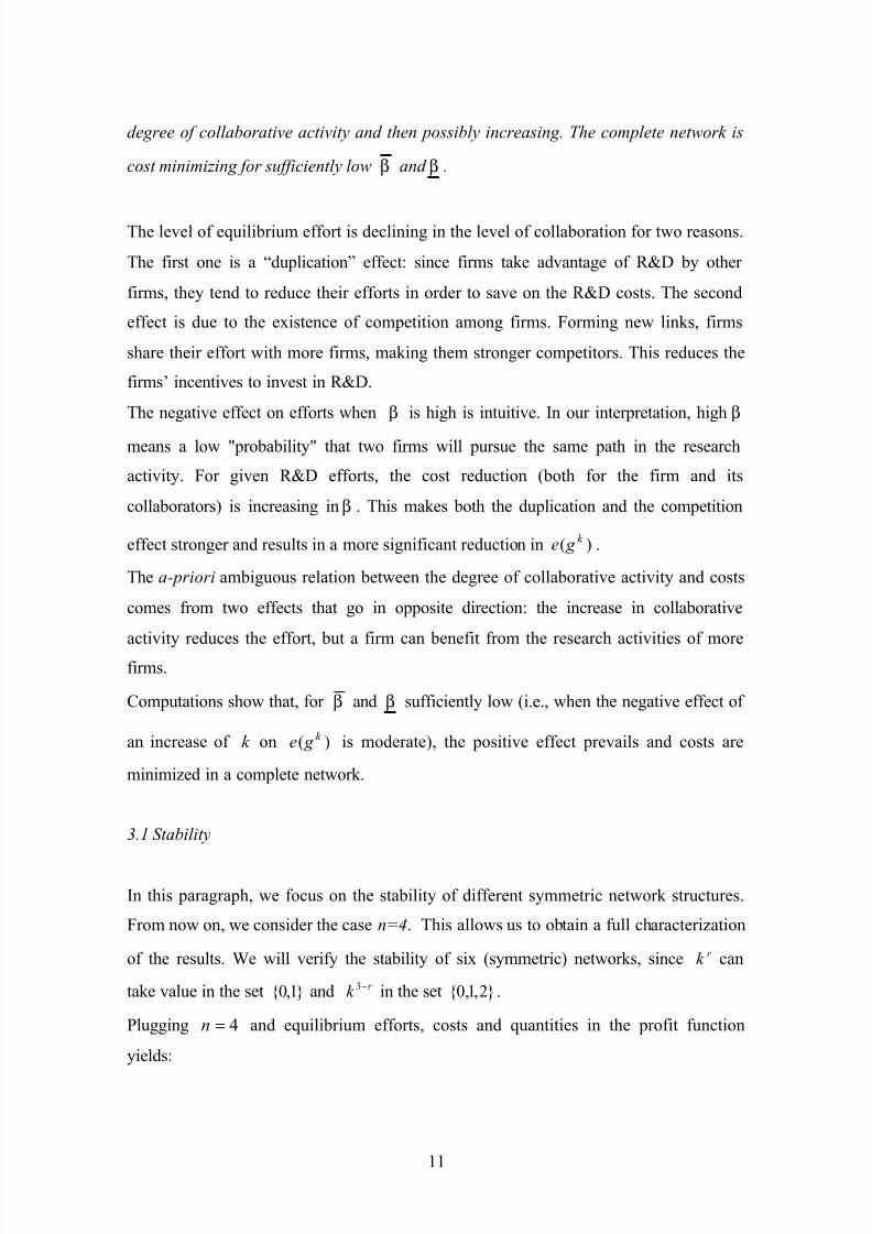
degree of collaborative activity and then possibly increasing. The complete network is

cost minimizing for sufficiently low β and β .

The level of equilibrium effort is declining in the level of collaboration for two reasons.

The first one is a “duplication” effect: since firms take advantage of R&D by other

firms, they tend to reduce their efforts in order to save on the R&D costs. The second

effect is due to the existence of competition among firms. Forming new links, firms

share their effort with more firms, making them stronger competitors. This reduces the

firms’ incentives to invest in R&D.

The negative effect on efforts when β is high is intuitive. In our interpretation, high β

means a low "probability" that two firms will pursue the same path in the research

activity. For given R&D efforts, the cost reduction (both for the firm and its

collaborators) is increasing in β . This makes both the duplication and the competition

effect stronger and results in a more significant reduction in )( k g e .

The a-priori ambiguous relation between the degree of collaborative activity and costs

comes from two effects that go in opposite direction: the increase in collaborative

activity reduces the effort, but a firm can benefit from the research activities of more

firms.

Computations show that, for β and β sufficiently low (i.e., when the negative effect of

an increase of k on )( k g e is moderate), the positive effect prevails and costs are

minimized in a complete network.

3.1 Stability

In this paragraph, we focus on the stability of different symmetric network structures.

From now on, we consider the case n=4. This allows us to obtain a full characterization

of the results. We will verify the stability of six (symmetric) networks, since r k can

take value in the set }1,0{ and r k −3 in the set }2,1,0{ .

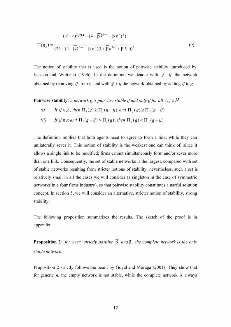
Plugging 4=n and equilibrium efforts, costs and quantities in the profit function

yields:



12

233

232

))1)(4(25(

))4(25()(

)(r r r r

r r

k k k k k

k k c A

g

−

−

−

−

−

−

++−−−

−−−−

=Πββββ

ββ

(9)

The notion of stability that is used is the notion of pairwise stability introduced by

Jackson and Wolisnki (1996). In the definition we denote with ij− the network

obtained by removing ij from g , and with ij+ the network obtained by adding ij to g .

Pairwise stability: A network g is pairwise stable if and only if for all ji ∈,

(i) If ij ∈ , then )()( ij g g ii −Π≥Π and )()( ij g g j j −Π≥Π

(ii) If ij ∉ and )()( g ij g ii Π>+Π , then )()( ij g g j j +Π<Π

The definition implies that both agents need to agree to form a link, while they can

unilaterally sever it. This notion of stability is the weakest one can think of, since it

allows a single link to be modified: firms cannot simultaneously form and/or sever more

than one link. Consequently, the set of stable networks is the largest, compared with set

of stable networks resulting from stricter notions of stability; nevertheless, such a set is

relatively small in all the cases we will consider (a singleton in the case of symmetric

networks in a four firms industry), so that pairwise stability constitutes a useful solution

concept. In section 5, we will consider an alternative, stricter notion of stability, strong

stability.

The following proposition summarizes the results. The sketch of the proof is in

appendix:

Proposition 2: for every strictly positive β and β , the complete network is the only

stable network.

Proposition 2 strictly follows the result by Goyal and Moraga (2001) They show that

for generic n, the empty network is not stable, while the complete network is always



13

stable. It can be shown that this result holds also in our model. They also show that for

n=4, the complete network is the only symmetric stable network, as it is the case here.

Then, no matter what are the degrees of technological opportunities and technological

heterogeneity, firms have always the incentive to “destabilize” a symmetric network

different from the complete network, forming a new link. Starting from a situation in

which firms are symmetric, firms which form a new link can create an asymmetric

market structure by sharing their R&D effort. In all the cases this leads to some

reduction in costs, even if links occur between firms in the same technological group,

for which information sharing may be not very effective. The complete network is

stable because in this case, by definition, it is not possible to form new links, and firms

do not find convenient to sever one of their links, weakening their competitive position.

3.2 Aggregate profits

In this section, we consider the behavior of different symmetric networks in terms of

aggregate profits. We try to assess the relation between the incentive for individual

firms to form collaborative links and what is desirable for them collectively. Since insymmetric networks all firms obtain the same level of profits, it is sufficient to compare

equilibrium profits for the all possible network structures (denoted with )( k g Π , where

the subscript is omitted for symmetry), in the range of all conceivable values of β

and β . Proposition 3 summarizes the results.

Proposition 3: define )()(),()2,0()2,1(

1 g g H Π−Π=ββ . For all β and β such

that 0),(1 >ββ H , the complete network maximizes aggregate profits. Otherwise, a

network in which all the firms are linked with and only with the firms of the other

technological group ( 2,0 3 == −r r k k ) maximizes aggregate profits. In economic terms,

the complete network is optimal for firms collectively when technological opportunities

are not “too high”.



14

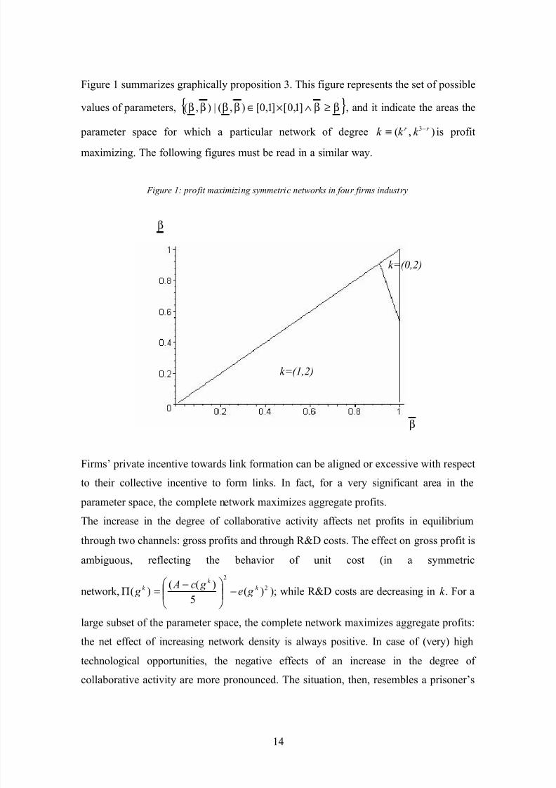
Figure 1 summarizes graphically proposition 3. This figure represents the set of possible

values of parameters, { }ββββββ ≥∧×∈ ]1,0[]1,0[),(|),( , and it indicate the areas the

parameter space for which a particular network of degree ),( 3 r r k k k −

≡is profit

maximizing. The following figures must be read in a similar way.

Figure 1: profit maximizing symmetric networks in four firms industry

β

β

Firms’ private incentive towards link formation can be aligned or excessive with respect

to their collective incentive to form links. In fact, for a very significant area in the

parameter space, the complete network maximizes aggregate profits.

The increase in the degree of collaborative activity affects net profits in equilibrium

through two channels: gross profits and through R&D costs. The effect on gross profit is

ambiguous, reflecting the behavior of unit cost (in a symmetric

network, 2

2

)(5

)(()( k

k k g e

g c A g −

−=Π ); while R&D costs are decreasing in k . For a

large subset of the parameter space, the complete network maximizes aggregate profits:

the net effect of increasing network density is always positive. In case of (very) high

technological opportunities, the negative effects of an increase in the degree of

collaborative activity are more pronounced. The situation, then, resembles a prisoner’s

k=(0,2)

k=(1,2)



15

dilemma. While firms would collectively prefer a lower degree of collaboration,

individually they have the incentive to destabilize a symmetric network in order to alter

market structure in their favour. This results in a Pareto dominated situation.

3.3 Welfare Analysis

While the previous section has considered the collective incentives for firms to form

collaborative links, this section takes into account social welfare, as defined by equation

(4).

Proposition 4: define

)()(),()2,0()1,1(

2 g W g W H −=ββ

)()(),( )2,1()2,0(

3 g W g W H −=−ββ

It can be shown that 0),(2 >ββ H implies 0),(3 >ββ H , and 0),(3 <ββ H implies

0),(2 <ββ H .

For all β and β such that 0),(2 >ββ H , the network where all firms have one link

inside and one link outside their technological group ( 1,1 3 == −r r k k ) is welfare

maximizing. For all β and β such that ),(0),( 23 ββββ H H >> , the network where

all firms have two links outside and zero link inside their technological group

( 2,0 3 == −r r k k ) is welfare maximizing. Finally, if 0),(3 <ββ H , the complete network

is welfare maximizing .



16

Figure 2: Welfare maximizing symmetric networks

β

β

When technological opportunities are low, the complete network is welfare maximizing,

and social interests and firms’ private incentives coincide. Social welfare depends on

the degree of collaborative activity through its effect on profits and through the totalquantity produced, which determines consumer surplus and it is inversely related to the

unit cost of production. When technological opportunities are low, the net effect of an

increase in the degree of collaborative activity is always positive, and maximal

information sharing is optimal. When technological opportunities increase, a less dense

network becomes more desirable from a social point of view, because the negative

effects from an increased degree of collaboration are higher than in the previous case.

Although )2,0(=k and )1,1(=k are equally dense, the latter is socially preferred for

very high technological opportunities. This happens because this structure minimizes

the negative effects of an increase of k on equilibrium effort: as shown by Proposition 1,

such a negative effect is higher when β is higher, and so it can socially optimal to

“substitute” a link outside firms’ technological group with a link inside firms’

technological group.

k=(0,2)

k=(1,1)

k=(1,2)



17

Finally, it is worth noting that the area of the parameter space for which welfare is

maximized by a complete network is included in the area of the parameter space for

which aggregate profits are maximized by a complete network. In other words, when

the complete network is social welfare maximizing, it is also profit maximizing, but the

converse is not true. This is because, when considering social welfare, one needs to add

the possibly negative effect that an increase in k generates for consumer surplus,

through the reduction of total quantity produced due to higher production costs.

3.4 Discussion

The analysis of symmetric networks has shown that the results of Goyal and Moraga in

terms of stability are not significantly modified by introducing a role for technological

opportunity and technological heterogeneity: the complete network is the only

symmetric stable network, independently from β and β . Firms have always the

incentive to alter a symmetric architecture (resulting in an asymmetric market structure)

by forming a new link, whenever this is possible.

With respect to networks that maximize aggregate profits and social welfare, we do not

find that individual incentives towards link formation are necessarily excessive, as in

Goyal and Moraga. Actually, the complete network maximizes aggregate profits for a

large set of parameters, while, if technological opportunities are sufficiently low, it is

optimal also both from the society point of view to have maximal information sharing.

A more specific role for technological heterogeneity is clearly seen comparing the

results about pairwise stability and social welfare. There is an area of the parameter

space, where both technological heterogeneity and technological opportunities are high,

in which it is socially optimal that information sharing occurs only when it is more

effective, that is among firms in different technological groups. However, firms aiming

at capturing strategic positions in the network (and consequently a competitive

advantage in the industry) have the incentive the share their efforts with firms in their

same technological group, which is detrimental in terms of the “collective” incentives to

invest in R&D. This leads to a network which is denser that the social optimum.



18

4. Asymmetric networks

The analysis in section 3 has restricted the attention only to symmetric network. In this

section we extend the analysis to the properties of asymmetric networks. We will

develop the simplest case of n=3. This will lead us to consider a situation where

technological groups have different size. We shall assume that firm 1 belongs to group

1, while firms 2 and 3 belong to group 2.

Technological groups that are asymmetric in size represent an interesting case because

we can study if and how the firm in the smaller group (which possesses technological

capabilities that are unique in the context of the industry) can exploit this situation and

obtain an advantageous position in the network and in the market.

We need to compare six typologies of networks:

1.

The empty network, denoted with ∅ . In this case all the firms gain in

equilibrium the same profit, which we indicate with ∅Π1 .

2. The partially connected network of type 1, where there is one link between firm

1 and one firm in the other technological group (say firm 2). This network is

denoted with p1, and we indicate with 11 pΠ , 1

2 pΠ and 1

3 pΠ profits in equilibrium

for firm 1,2 and 3 respectively.

3. The partially connected network of type 2, where there is one link between the

two firms in the same technological group. This network is denoted with p2, and

equilibrium profits are 2

1

pΠ and 2

2

pΠ for firm 1 and firm 2 respectively (the

positions of firms 2 and 3 are symmetric).

4. The star network of type 1, where firm 1 is the hub (i.e. it is connected both

with firm 2 and firm 3) and firm 2 and firm 3 are the spokes (they are connected

only to firm 1). This network is denoted with st1, and equilibrium profits are

2

1

st Π and 2

2

st Π for firm 1 and firm 2 respectively (again, the positions of firms 2

and 3 are symmetric).

5. The star network of type 2, where say firm 2 is the hub and the remaining firms

are the spokes. This network is denoted with st2, and we indicate with

2

1

st Π , 2

2

st Π and 2

3

st Π profits in equilibrium for firm 1, 2 and 3 respectively.



19

6.

The complete network, denoted with c. We indicate with c

1Π and c

2Π

equilibrium profits for firm 1 and 2 respectively (the positions of firms and 3 are

symmetric).

4.1 Stability

The next proposition summarizes the results about stability. Goyal and Moraga shows

that two kinds of structures are possibly stable, when spillovers outside collaboration

are absent as in our model: the partially connected network and the complete network.

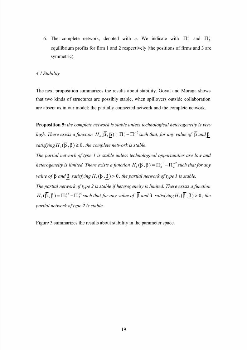
Proposition 5: the complete network is stable unless technological heterogeneity is very

high. There exists a function2

114 ),( st c

H Π−Π=ββ such that, for any value of β and β

satisfying 0),(4 ≥ββ H , the complete network is stable.

The partial network of type 1 is stable unless technological opportunities are low and

heterogeneity is limited. There exists a function2

2

1

25 ),( st p

H Π−Π=ββ such that for any

value of β and β satisfying 0),(5 >ββ H , the partial network of type 1 is stable.

The partial network of type 2 is stable if heterogeneity is limited. There exists a function

2

2

2

26 ),( st p

H Π−Π=ββ such that for any value of β and β satisfying 0),(6 >ββ H , the

partial network of type 2 is stable.

Figure 3 summarizes the results about stability in the parameter space.



20

Figure 3: stability in the three firms industry

β

β

Introducing firms’ heterogeneity does not impact on the types of networks that are

possibly stable, but the stability of different network structures does depend on β and

β .

Star networks are never stable. In particular firm 1 will not use its “special” position to

become the hub of a star. The star of type 1 is not stable because of two possible

deviations.

First, given the existence of a link between firm 1 and firm 2, firm 1 and firm 3 never

agree in maintaining a collaborative link. Firm 1 is willing to form a link for low β

(β <0.35). In this case, given that the opportunity of avoiding duplication of efforts is

limited, firm 1 does not find the strategy of an exclusive alliance with firm 2 attractive,

and it would rather collaborate also with firm 3. At the same time, firm 3 is willing to

cooperate with 1 only when β is sufficiently high ( β >0.48). Forming an alliance with

1, firm 3 obtains access to firm 1’s R&D effort, but it makes firm 1 even stronger. It

turns out that the first effect prevails for β high.

A second profitable deviation is given by firm 2 and firm 3 forming a link. In this case

they can make their position stronger in market competition vis-à-vis firm 1, by sharing

their R&D efforts.

(c,p1,p2)

(c,p1)

c(p1)



21

In partially connected network of type 1, the position of firm 1 is not “special”, in the

sense that it obtains the same level of profit as the firm it is connected with. However,

whenever heterogeneity is above a minimum threshold (such that we are not in the

range in which the partially connected network of type 1 is stable) firm 1 can obtain the

maximum industry profit in any stable network.

Firms in the relatively “crowded” technological group, instead, show more variability in

the profits associated to stable networks.

4.2 Aggregate profits

This section considers how aggregate profits vary as a function of the network. In this

case it is necessary to sum the profits of the three firms, since it is not possible to talk

about a representative firm in the industry (apart from the special case of the empty

network)

Define: )()()()( 321 g g g g Π+Π+Π=Π , with { }∅∈ ,2,1,2,1, st st p pc g .

Proposition 6: when the technological opportunities are sufficiently high, the partially

connected network of type 1 maximizes profits; otherwise the complete network does.

There exists a function )1()(),(7 pc H Π−Π=ββ such that, for any value of β and β

satisfying 0),(7 >ββ H , the complete network maximizes aggregate profits.

Figure 4 summarizes the results.



22

Figure 4: profit maximizing networks in three firms industry

β

β

When technological opportunities are high (in particular, when information sharing

between technologically heterogeneous firms is effective), allied firms have a strong

incentive to invest in R&D and waken the position of the remaining firm in marketcompetition. Then, their costs are low, and their profits high. Although unevenly

distributed, aggregate profits in the partially connected network turn out to be higher

than in the complete network.

4.3 Social Welfare

Finally, we consider the social welfare properties of networks in a three firms’ industry.

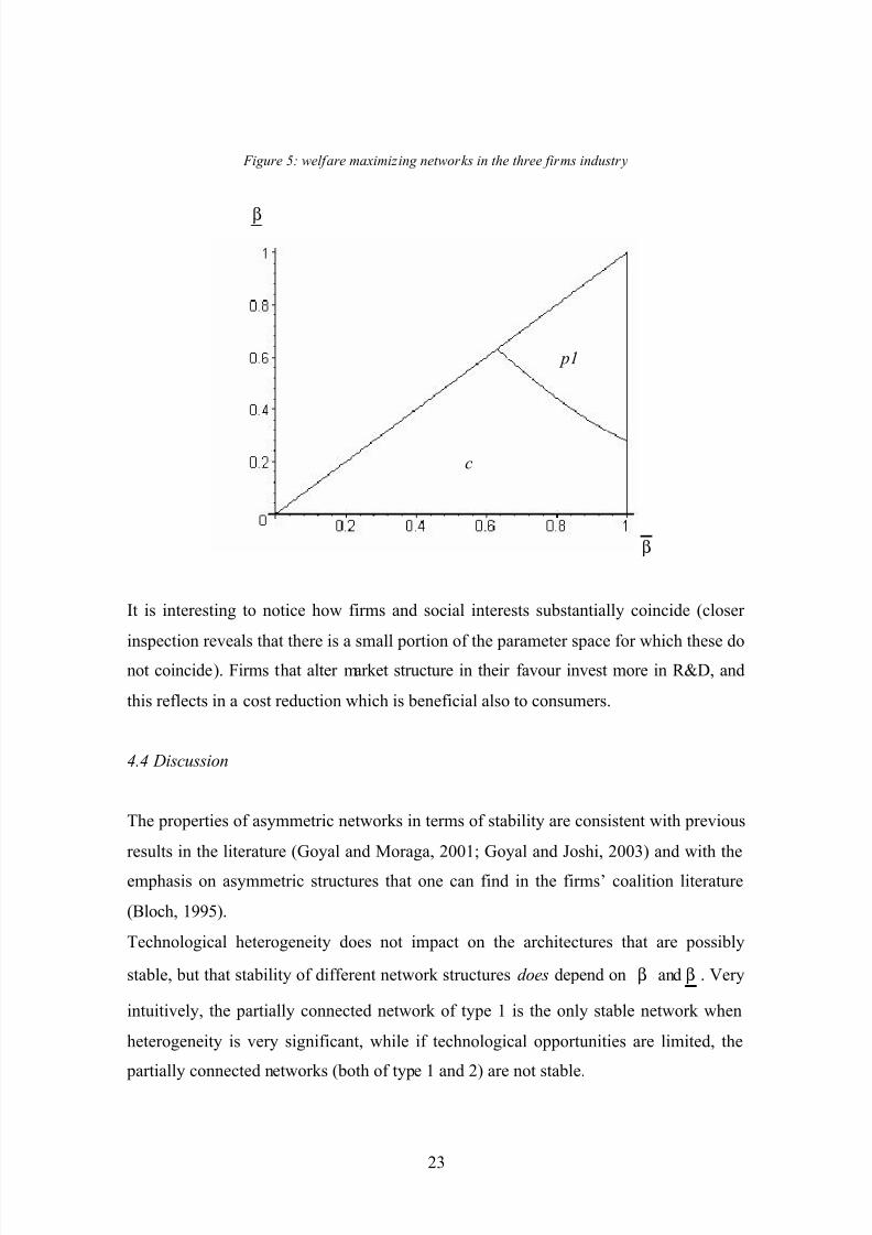
Proposition 7: social welfare is maximized by a partially connected network of type 1

whenever technological opportunities are sufficiently high. Otherwise the complete

network maximizes social welfare. There exists a function )1()(),(8 pc H Π−Π=ββ

such that, for any values of β and β satisfying 0),(8 >ββ H , the complete network

maximizes social welfare.

p1

c



23

Figure 5: welfare maximizing networks in the three firms industry

β

β

It is interesting to notice how firms and social interests substantially coincide (closer

inspection reveals that there is a small portion of the parameter space for which these donot coincide). Firms that alter market structure in their favour invest more in R&D, and

this reflects in a cost reduction which is beneficial also to consumers.

4.4 Discussion

The properties of asymmetric networks in terms of stability are consistent with previous

results in the literature (Goyal and Moraga, 2001; Goyal and Joshi, 2003) and with the

emphasis on asymmetric structures that one can find in the firms’ coalition literature

(Bloch, 1995).

Technological heterogeneity does not impact on the architectures that are possibly

stable, but that stability of different network structures does depend on β and β . Very

intuitively, the partially connected network of type 1 is the only stable network when

heterogeneity is very significant, while if technological opportunities are limited, the

partially connected networks (both of type 1 and 2) are not stable.

p1

c



24

Firm 1, which is the unique firm belonging to its technological group, does not gain a

prominent role in any stable networks. Nevertheless, it obtains the highest profit in the

complete network and it can be excluded in pairwise stable networks only in the limited

range of parameters where technological opportunities are high and technological

heterogeneity is low.

Comparing networks that are pairwise stable and networks maximizing aggregate

profits and social welfare, one can observe that in general at least one stable network (if

the set of stable networks is not a singleton) is efficient, from firms’ and social point of

view. The exception is the range in which the partially connected network of type 1 is

the only stable network, where profits and social welfare are maximized by a complete

network.

5 Strong stability in symmetric and asymmetric networks

In this section, we apply a stronger notion of stability to the two cases studied in the

sections 3 and 4. As we said, pairwise stability is a weak notion of stability, because it

considers as admissible only a small set of deviations. In particular, it does not allow for

coordinated actions of agents that form or sever more than one link. In contexts wherethe number of agents is small, it seems plausible that agents can arrange more complex

deviations, to which a network must resist to be considered as stable.4

The notions we will use is the notion of strongly stable networks, discussed in Jackson

and van den Nouweland (2003) and Dutta and Mutuswami (1997). In words, a network

is strongly stable if there are no coalitions of players that by forming or severing links

can strictly increase the payoff of the members of the coalition, where members of the

coalition can add links only among them, but they can sever links with all the agents in

the network.

4 In an alternative approach, one could consider network formation as a noncooperative game, in line with

Myerson (1991). Firms simultaneously propose the subset of agents they want to be connected with, and

links are formed only when the proposals are reciprocated. However, Nash equilibrium is too weak as a

solution of concept, due to the coordination problem that arises for the required double coincidence of

wants for the formation of a link. The refinement of undominated Nash equilibrium, which is sometimes

used in the literature (Goyal and Joshi, 2003), is not of particular help here, because only the empty set as

a strategy is weakly dominated for all the parameters values. In the four firms industry, all the symmetric

networks can be sustained as Nash equilibrium of the link formation game, and all the symmetric

networks but the empty network can be sustained as undominated Nash equilibrium for some range of the

parameters. Finally, it is worth noting that the notion of strongly stable networks we discuss in the textcoincides with the notion of strong Nash equilibrium in the link formation game.



25

Formally, strong stability is defined as follows:

Strong stabil ity : define N S ⊆ as a coalition in N. A network ′ is obtainable from g

via S if:

(i) ij ′∈ and ij ∉ implies S ji ⊂},{ .

(ii) ij ∈ and ij ′∉ implies ∅≠∩ S ji },{ .

A network g is strongly stable if there are no coalitions S and network ′ obtainable

from g via S for which )()( g g ii Π>′Π , for all S i ∈ .

This definition of stability is strict, and consequently the existence of strongly stable

networks is not guaranteed. When existing, strongly stable networks have nice

properties. In particular, strongly stable networks are by definition Pareto efficient. The

definition of strong stability that we use here (which is taken from Dutta and

Mutuswami, 1997) does not imply pairwise stability as defined in section 3 (which is

the original definition by Jackson and Wolinski, 1996): in the former, establishing a

new link is an admissible deviation only if both firms are strictly better off; in the latter,

one agent can be weakly better off. However, the implication does not hold only for

parameters values that constitute the borders between areas of stability of different

network structures.5

5.1 Strong stability in the four firms’ industry

In the case of four firms, only one symmetric network turns out to be pairwise stable.

Then, we simply need here to verify if (and when) the complete network, which is

always pairwise stable, is also strongly stable.

The results are summarized in proposition 8. In proving Proposition 3, we will refer to a

particular asymmetric structure, the triangle (denoted with tr ), where we have a fully

connected component of three firms (say 1, 3 and 4, with 3 and 4 belonging to the same

5

We will show in the next subsections why is preferable to adopt this version of strong stability. Anotheralternative would be to modify the definition of pairwise stability, again with minor differences.



26

technological group) and one firm (firm 2) is isolated. In equilibrium, profits are

)(and)(),( 321 tr tr tr ΠΠΠ (the positions of firm 3 and 4 are symmetric).

Proposition 8: the complete network is almost never strongly stable, except that for

very low technological opportunities or very high technological heterogeneity. There

exists a function )()(),( )2,1(

39 g tr H Π−Π=ββ such that, for all the values of β and β

for which 0),(9 >ββ H the complete network is not strongly stable.

Figure 6: strongly stable networks in the four firms industry

β

β

Proposition 8 is very close to a non-existence result: for a largely predominant subset

part of the parameter space, the complete network is not strongly stable, so that there are

no symmetric networks that are strongly stable. Nevertheless, the result has interesting

economic implications for the nature of the coalition and the deviation that turns out to

be profitable. Except that for a very limited small area in the parameter space, three

firms have the incentive to sever jointly their links towards the fourth firms, creating an

asymmetric market structure where three, “networked” firms have a dominant position

in the product market. In particular, while firm 1 (which is the only firm in its

technological group to have connections) always prefers to be in the triangle network,

k=(1,2)k=(1,2)



27

firm 2 and firm 3 do for the range of parameters shown in the figure. Furthermore, when

β and β are sufficiently high, the isolated firms is forced out of the market )0( 2 =q .

This result is interesting because it confirms the importance of asymmetric network

structures, as shown by the three firms’ analysis, and the role played by collaborative

ventures in creating ex post asymmetries in ex ante symmetric situations. A natural

question then is when the triangle network turns out to be pairwise stable. It can be

shown that for a significant range of parameters (in particular, when technological

opportunities are high or technological heterogeneity is high) the triangle network is not

pairwise stable because connected firms prefer to form the link with the isolated firm.6

This leads towards the formation of a complete network, where profits for such firms

are generally lower. Although the model is purely static, it suggests a dynamic story in

which firms have the private incentive to form very dense networks, but then they have

the “collective” incentive to sever the links towards one firm, to exclude it from the

network and create an asymmetric market structures. This has two consequences: it

suggests instability of cooperative ventures, and a cycle in alliances formation. Both

aspects are consistent with empirical evidence (Kogut, 1988; Hagedoorn, 2002).

5.2 Strong stability in the three firms’ industry

In the case of three firms, three structures turn out to be pairwise stable: the complete

network, the partially connected network of type 1 and the partially connected network

of type 2.

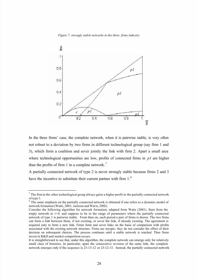
Proposition 9 summarizes the results about strong stability in the three firms’ industry.

Proposition 9: the partially connected network of type 2 is never strongly stable. The

partially connected network of type 1 is always strongly stable, when is pairwise stable.

The complete network is strongly stable only when technological opportunities are low.

There exists a function )()1(),( 1110 c p H Π−Π=ββ such that the complete network is

strongly stable for all values of β and β for which 0),(10 <ββ H .

6 The graphical representation of pairwise stability for the triangle network is reported in the appendix.



28

Figure 7: strongly stable networks in the three firms industry

β

β

In the three firms’ case, the complete network, when it is pairwise stable, is very often

not robust to a deviation by two firms in different technological group (say firm 1 and

3), which form a coalition and sever jointly the link with firm 2. Apart a small area

where technological opportunities are low, profits of connected firms in p1 are higher

than the profits of firm 1 in a complete network.7

A partially connected network of type 2 is never strongly stable because firms 2 and 3

have the incentive to substitute their current partner with firm 1. 8

7 The firm in the other technological group always gains a higher profit in the partially connected network

of type 1.8 The same emphasis on the partially connected network is obtained if one refers to a dynamic model of

network formation (Watts, 2001; Jackson and Wat ts, 2002).

Consider the following algorithm for network formation, adapted from Watts (2001). Start from the

empty network at t=0, and suppose to be in the range of parameters where the partially connected

network of type 1 is pairwise stable. From then on, each period a pair of firms is drawn. The two firms

can form a link between them, if not existing, or sever the link, if already existing. The agreement is

required only to form a new link. Firms form and sever links on the basis of comparison with profits

associated with the existing network structure. Firms are myopic: they do not consider the effect of their

decision on subsequent choices. The process continues until a stable network is reached. Then firms

invest in R&D and market competition occurs.

It is straightforward to see that, under this algorithm, the complete network can emerge only for relatively

small class of histories. In particular, apart the consecutive revision of the same link, the completenetwork emerges only if the sequence is 23-13-12 or 23-12-13. Instead, the partially connected network

p1

p1

p1 p1

c



29

The partially connected network of type 1 is always strongly stable, because there are

no deviations that can make any pair of agents strictly better off. Moreover, firm 2 has

no incentive to move to a complete network either. 9

The analysis of strongly stable networks clearly points out the partially connected of

type 1 as a natural solution for the process of network formation. This is interesting for

several reasons.

First, on the empirical side, the special role played by this asymmetric network is

consistent with the empirical analysis that underlies the motive of altering market

structure as an important rationale for interfirm technological agreements (Hagedoorn,

1993). Also the results from the analysis of the four firms’ case are in line with this

evidence.

Second, the firm in group 2 that “succeeds” in forming the link obtains an advantage in

terms of profits, a gain this is increasing in βv

. This leads naturally to consider the strong

competition occurring between the two firms in the larger technological group. There

are two ways to tackle this issue. First, one can take the model as it is and solve the

problem of multiple equilibria invoking a role for “historical accidents” and path-

dependence, in a way that is similar to the one in Zirulia (2004). “Random” events (like

social contacts or geographical proximity) leads one firm in group 2 to form a link with

1, with long lasting effects on firms’ performance. It is interesting to observe that some

business scholars (for instance, Gulati et al., 2000) have underlined the importance for

firms to “rush” and form alliances with the “right” partners in the early phases of

technological or industrial cycles. Our simple model is consistent with this view. The

second solution is to explicitly model such a competition, supposing for instance a role

for side payments that allows firm 1 to exploit its strong bargaining power. If side- payments are allowed, we can expect that the firm excluded by the network would

"undercut" the other firm, transferring part of the surplus of being connected to firm 1.

of type 1 is immediately obtained whenever the first two firms forming a link are firms 1 and 2 or firms 2

and 3.

9 If one uses a notion of strong stability where agents in a deviating coalition may be weakly better off,

the partially connected network of type 1 is never strongly stable, because the coalition of 1, which isindifferent between the two partners, and the excluded partner from the network is winning.



30

In this view, firm 1 would exploit the “scarcity” of its technological resources in terms

of performance also under this architecture.

Third, in terms of policy, we can observe how the partially connected network is

welfare maximizing only when technological opportunities are high. There is a

significant area in the technological space (with high technological heterogeneity)

where welfare is maximized by the complete network. If technological opportunities are

not too high, a dense network is not detrimental to R&D efforts, and consequently it has

beneficial effects on consumer surplus. However, firms have the incentive to alter

market structure in their favor, excluding one firm from the network. In this case, there

is possibly room for public intervention to favor industry-wide cooperation.

6. Conclusions and plan for future work

The goal of this paper was to extend the analysis of R&D network formation in a setting

when technological heterogeneity among firms is considered. First (Section 3 and 4),

the results were derived in terms of pairwise stability, aggregate profits and social

welfare associated with different network structures. We wanted to consider the

robustness of Goyal and Moraga’s results to a modification that seems empiricallyrelevant. We consider two classes of networks. First, we consider symmetric networks

in a four firms industry. The complete network is always the only symmetric stable

network. Firm have always the incentive of altering the market structure adding a new

link, when network is not complete. Aggregate profits and social welfare are also

maximized by a complete network, if technological opportunities are not too high, so

that private and social incentives are aligned in these cases. Otherwise, less dense

networks are optimal from firms’ and society point of view. In the class of asymmetric

networks, for which the analysis has been performed in the case of three firms,

technological heterogeneity matters. Only the complete and the partially connected

networks are possibly stable, but which network is stable actually depends on the level

of heterogeneity and technological opportunities. Firms belonging to the smaller

technological group (having unique technological resources) obtain a special position in

the industry, since they can guarantee the maximum profits in the industry in every

stable network. The complete and partially connected networks are also the possible



31

welfare and aggregate profit maximizing networks, but social and private incentives do

not generally coincide. When technological opportunities are high, the partially

connected network involving two firms of different technological groups is pairwise

stable and it maximizes aggregate profits and social welfare.

In section 5, we consider the refinement of strong stability, where all the possible

deviations by coalitions of agents are allowed. It turns out that, in the four firms’ case,

the complete network is very rarely strongly stable, because a coalition of three firms

has the incentive to isolate the fourth firm and create an asymmetric market structure. In

the three firms’ case, the partially connected network where two firms in different

technological group are linked is for a large subset of parameter space the only strongly

stable network.

In this paper we made a number of restrictive assumptions. In particular, we considered

the role of technological heterogeneity independently from the nature and intensity of

competition and we kept the assumptions of homogenous good and Cournot

competition. Furthermore, we consider a simple representation of technological

heterogeneity, allowing only for two types of firms. For the future, we plan to develop a

model where firms are located in a technological space that affects both the intensity ofcompetition and the effects of information sharing, and study the stability and efficiency

properties of the networks as a function of firms’ localization.

Acknowledgments : This paper is a slightly modified version of the second chapter

from my PhD thesis. I thank Franco Malerba, Pierpaolo Battigalli, Robin Cowan,

Nicoletta Corrocher and the participants to a seminar in Milan, Bocconi University,

June 2004, for useful comments on a previous version. The usual disclaimers apply.



32

References

d’Aspremont, C. and Jacquemin, A. (1988), “Cooperative and noncooperative R&D in

duopoly with spillovers”, American Economic Review, 78,1133-1137.

Bloch, F. (1995), "Endogenous structures of Association in Oligopolies" RAND Journal

of Economics, 26,537-556.

Cohen, W. and Levinthal, D. (1989), “Innovation and learning: the two faces of

Research and development”, The Economic Journal , 99, 569-596.

Dutta, B. and Mutuswami, S. (1997), “Stable networks”, Journal of Economic Theory,

76,322-344.

Goyal, S. and Joshi, S. (2003), “ Networks of Collaboration in oligopoly , Games and

Economic behavior,43 , 57-85.

Goyal, S and Moraga, J. (2001), “R&D Networks”, RAND Journal of Economics, 32,

686-707.

Goyal, S. and Konovalov, A. and Moraga, J. (2004), "Hybrid R&D", mimeo.

Gulati, R Nohria, N. and Zaheer, A. (2000), “Strategic networks”, Strategic

management Journal 21, 203-215.

Hagedoorn, J. (1993), "Understanding the rationale of strategic technology partnering:

inter-organizational modes of cooperation and sectoral differences" Strategic

management Journal , 14, 371-385.



33

Hagedoorn, J. (2002), "Inter-firm R&D partnerships: an overview of major trends and

patterns since 1960", Research Policy, 31,477-492.

Jackson, M. and Watts, A. (2002), “The evolution of social and economic networks”

Journal of economic theory, 106, 265.-295.

Jackson, M. and Wolinski, A. (1996), “A Strategic Model of Social and Economic

Networks”, Journal of Economic Theory, 71, 44-74.

Jackson, M. and van den Nouweland, A. (2003), “Strongly Stable Network”, Games

and Economic Behavior , forthcoming.

Kamien, M. Mueller, M. and Zang, I. (1992), “Research joint ventures and R&D

cartels”, American Economic Review, 82, 1293-1306.

Katz, M. (1986), “An analysis of cooperative research and development”, RAND

Journal of Economics, 17, 527-543.

Kogut, B. (1988) “Joint ventures: theoretical and empirical perspectives”, Strategic

Management Journal , 9, 319-332.

Mariti, P and Smiley, R. (1983), "Cooperative agreements and the organization of

industry", The Journal of Industrial Economics, 31, 437-451.

Myerson, R. (1991) “Game Theory: Analysis of Conflict”. Harvard University Press.

Nelson, R. and Winter, S. (1982), "An evolutionary theory of economic change",

Harvard University Press, Cambridge (MA).



34

Powell, W.W., Koput, K.W. and Smith-Doerr, L. (1996), “Interorganizational

collaboration and the locus of innovation: networks of learning in biotechnology”

Administrative Science Quarterly, 41, 116-145.

Suzumura, K.(1992), ”Cooperative and noncooperative R&D in an oligopoly with

spillovers” American Economic Review, 82, 1307-1320.

Watts, A. (2001)”A dynamic model of network formation”, Games and economic

behavior , 34, 331-341.

Zirulia, L. (2004) "The evolution of R&D networks", MERIT-Infonomics Research

Memorandum, n°007.

Appendix

Proof of Pr opositi on 1:

The proposition immediately derives from the following expression. Symmetric expression holds forr k

−3:

0)1)(()1)][(1)(()1[(

))(()(

)()(

332332

33

),1(),( 33

>−++−−−+−+−−−+

+−−−−−

=−

−−−−

−−

+ −−

βββββββββ

ββββββr r r r r r r r

r r r r

k k k k

k k k k nnk k k k nn

k k nk k nc A

g e g er r r r

)1)(()1)][(1)(()1[(

)122()1)((

)()(

332332

32

),1(),( 33

βββββββββ

ββββr r r r r r r r

r r

k k k k

k k k k nnk k k k nn

k k nnc A

g c g cr r r r

−++−−−+−+−−−+−−−−+−

=−

−−−−

−

+ −−

which is positive only for 01223 >++−− −

βββr r

k k n

and finally,

0)1)(()1(

])(()1[()(332

332

<−+−−−+

++−−−+−−=

∂∂

−−

−−

ββββ

ββββ

β r r r r

r r r r r

i

k k k k nn

k k nk k nnk c Ae



35

Proof of Pr opositi on 2: Pairwise stabili ty of symmetri c networks in the four fi rms industry

We report here a sketch of the proof of this proposition. All the computations and the relevant plots have

been performed with the help of the software Maple, and they are available upon request (to:

[email protected]).

We assume, without loss of generality, that firm 1 and firm 2 belong to the same technological group 1,

and firm 3 and 4 belong to the technological group 2. Then, the procedure is as follows:

• For each network (apart from isomorphic networks) one need to consider all the deviations that

are considered in the notion of pairwise stability;

• this yields unit cost as a function of efforts for each firm, and consequently profit function;

• the first order conditions for representative firms (i.e. firms playing the same role in the network)

are computed;

• the system of first order conditions is solved, invoking symmetry of effort for firms playing the

same role in the network;

• equilibrium efforts are computed, and plugged into the profit function of deviating firms;

• equilibrium profits from the deviation and equilibrium profits in the symmetric network under

consideration are compared.

The complete network is stable

In this case, the only deviation one needs to take into account is when two firms sever one link. It can be

shown that independently fromβ , such a deviation is not profitable.

The empty network is not stable

In this case, the possible deviations are those where two firms form a link. It can be shown that for any

strictly positive value of β , such a deviation is profitable. Furthermore, if 51/2-3/2>β , the solution

is a corner solution where, for one isolated firm, e=0 and q=0 .

The network 1,1 3 == −r r k k is not stable

In this case, the deviation in which two firms belonging to different technological group, say firm 1 and 4,

form a link is profitable.








In this case, it can be shown that the deviation in which two firms belonging to the same technological

group, say firm 1and 2, form a link is profitable.



36

Proof of Propositi on 5: Pair wise stability in the three fi rms industry

In this case, we need to take into account six types of structures, and studying the incentives of firms to

move from one structure to other by forming or severing links.

Without loss of generality we assume that firm 1 belongs to technological group 1, while firm 2 and 3

belong to technological group 2. Computations show that:

The empty network is never stable

Any pair of firms has the incentive to form a link and moving to a partially connected network of type 1

or 2, for any strictly positive value of β .

A star network of type 1 is never stable

For any strictly positive value of β , firm 2 and firm 3 find convenient to form a link, and transform the

star 1 in a complete network.

A star network of type 2 is never stable

Expect that for high β and low β , firm 1 would prefer to form a link with firm 3 (which is always

willing to form such a link) and make the star network of type 2 a complete network. Furthermore, except

that for very low values both of β and β , firm 2 (supposed to be the hub in the star) wants to sever

the link with firm 3 and make the network a partially connected network of type 1. It can be shown that

the area in the parameter spaces for which the two deviations are not profitable do not intersect, so that

there is always a profitable deviation.

A complete network is stable unless β is very high and β is very low.

There is a range of values (as reported in the paper) for which firm 1 would prefer to severe the link say

with 3 and make the network a star of type 2. Firm 3 is never willing to sever such a link, while it is never

profitable for firm 2 and firm 3 to sever their link.

A partially connected network of type 1 is stable unless technological opportunities are low and

technological heterogeneity is limited.

In this case firm 1 and firm 3 never agree on forming the link between them (there are no values of β for

which the double coincidence of wants hold). Firm 2 and firm 3 agree on forming a link between them

(making the network a star of type 2) for the range of values of β and β specified in the paper.

Indeed, firm 3 is always willing to form such a link.

A partially connected network of type 2 is stable if technological opportunities are high and technological

heterogeneity is limited.

Firm 2 and 3 are never willing to sever their existing link. While firm 1 always agrees on forming a link

with say firm 2, firm 2 gives its consent only for the range shown in the paper.



Propositi on 9: Pair wise stabili ty of the tri angle network

Figure 8: Pairwise stability of the triangle network

β

β

tr

zirulia rd networks with heterogeneous firms.pdf

Documents