people.eecs.berkeley.eduzmccarthy/pdfs/bretl... · · 2016-02-03article quasi-static manipulation...

Article

Quasi-static manipulation of a Kirchhoffelastic rod based on a geometric analysisof equilibrium configurations

The International Journal ofRobotics Research2014, Vol 33(1) 48–68© The Author(s) 2013Reprints and permissions:sagepub.co.uk/journalsPermissions.navDOI: 10.1177/0278364912473169ijr.sagepub.com

Timothy Bretl1 and Zoe McCarthy2

AbstractConsider a thin, flexible wire of fixed length that is held at each end by a robotic gripper. Any curve traced by this wirewhen in static equilibrium is a local solution to a geometric optimal control problem, with boundary conditions that varywith the position and orientation of each gripper. We prove that the set of all local solutions to this problem over allpossible boundary conditions is a smooth manifold of finite dimension that can be parameterized by a single chart. Weshow that this chart makes it easy to implement a sampling-based algorithm for quasi-static manipulation planning. Wecharacterize the performance of such an algorithm with experiments in simulation.

KeywordsManipulation planning, manipulation, path planning for manipulators, manipulation, mechanics, design and control

1. Introduction

Figure 1 shows a thin, flexible wire of fixed length that isheld at each end by a robotic gripper. Our basic problemof interest is to find a path of each gripper that causes thewire to move between start and goal configurations whileremaining in static equilibrium and avoiding self-collision.As will become clear, it is useful to think about this problemequivalently as finding a path of the wire through its set ofequilibrium configurations (i.e. the set of all configurationsthat would be in equilibrium if both ends of the wire wereheld fixed).

There are two reasons why this problem seems hard tosolve. First, the configuration space of the wire has infinitedimension. Elements of this space are framed curves, i.e.continuous maps q : [0, 1] → S E( 3), the shape of which ingeneral must be approximated. Second, a countable num-ber of configurations may be in static equilibrium for givenplacements of each gripper, none of which can be com-puted in closed form. For these two reasons, the literature onmanipulation planning suggests exploring the set of equilib-rium configurations indirectly, by sampling displacementsof each gripper and using numerical simulation to approxi-mate their effect on the wire. This approach was developedin the seminal work of Lamiraux and Kavraki (2001) andwas applied by Moll and Kavraki (2006) to manipulation ofelastic “deformable linear objects” like the flexible wire weconsider here.

Our contribution in this paper is to show that the set ofequilibrium configurations for the wire is a smooth man-ifold of finite dimension that can be parameterized by a

single (global) coordinate chart. We model the wire as aKirchhoff elastic rod (Biggs et al., 2007). The framed curvetraced by this rod in static equilibrium can be described as alocal solution to a geometric optimal control problem, withboundary conditions that vary with the position and orienta-tion of each gripper (Walsh et al., 1994; Biggs et al., 2007).Coordinates for the set of all local solutions over all bound-ary conditions are provided by the initial value of co-statesthat arise in necessary and sufficient conditions for optimal-ity. These coordinates describe all possible configurationsof the elastic rod that can be achieved by quasi-static manip-ulation, and make manipulation planning—the seemingly“hard problem” described above—very easy to solve. Wewill provide both analytical and empirical results to justifythis claim in the context of a sampling-based planning algo-rithm. For now, we note that the computations ultimatelyrequired by our approach are trivial to implement.

A variety of applications motivate our work: knot tyingand surgical suturing (Hopcroft et al., 1991; Takamatsuet al., 2006; Wakamatsu et al., 2006; Saha and Isto,2007; Bell and Balkcom, 2008), cable routing (Inoue and

1Department of Aerospace Engineering, University of Illinois at Urbana-Champaign, USA2Electrical and Computer Engineering, University of Illinois at Urbana-Champaign, USA

Corresponding author:Timothy Bretl, Department of Aerospace Engineering, University of Illi-nois at Urbana-Champaign, 306 Talbot Lab, MC-236 104 South WrightStreet, Urbana, IL 61801, USA.Email: [email protected]

at UNIV CALIFORNIA BERKELEY LIB on February 3, 2016ijr.sagepub.comDownloaded from

http://ijr.sagepub.com/

Bretl and McCarthy 49

Inaba, 1985), folding clothes (van den Berg et al., 2011;Yamakawa et al., 2011), compliant parts handling (Linet al., 2000; Gopalakrishnan and Goldberg, 2005) andassembly (Asano et al., 2010), surgical retraction of tis-sue (Jansen et al., 2009), protein folding (Amato andSong, 2002), haptic exploration with “whisker” sensors thatare modeled as elastic rods (Clements and Rahn, 2006;Solomon and Hartmann, 2010), etc. We are also motivatedby the link, pointed out by Tanner (2006), between manipu-lation of deformable objects and control of hyper-redundant(Chirikjian and Burdick, 1995) and continuum (Ruckeret al., 2010; Webster and Jones, 2010) robots. However, weacknowledge that our work in this paper is theoretical andthat much remains to be done before any of it can be appliedin practice.

Section 2 gives a brief overview of prior approachesto quasi-static manipulation of “deformable linear objects”like the elastic rod. Section 3 provides an introduction to thekey ideas by consideration of a simpler example, namelyan elastic rod that is confined to a planar workspace. Sec-tion 4 establishes our theoretical framework. The two keyparts of this framework are optimal control on manifoldsand Lie–Poisson reduction. We derive coordinate formu-lae for necessary and sufficient conditions—in the formercase these formulae are well known, but in the latter casethey are not. Section 5 shows how our framework appliesto the Kirchhoff elastic rod. We prove that the set of allequilibrium configurations for this rod is a smooth manifoldof finite dimension that can be parameterized by a singlechart. Section 6 explains why this result makes the problemof manipulation planning easy to solve. Section 7 identifiesseveral limitations of our approach and suggests ways theselimitations might be addressed.

A preliminary version of this paper has appeared at a con-ference (Bretl and McCarthy, 2012). Several extensions areprovided here. The discussion of related work in Section2 and the consideration of a planar elastic rod in Section3 are both new, as are the physical interpretation of thecoordinate chart we derive (Section 5.4), the precise defi-nition of “straight-line paths” both in this chart and in thespace of boundary conditions (Section 5.5), the summaryof computations required by our approach, and the empir-ical results in simulation that we use to justify our choiceof local connection strategy (Section 6.2). In addition, weprovide a more direct proof of Lemma 4, which is the basisfor our main result in Section 5.2. Our ideas in this paperalso follow from, but significantly extend, earlier work on asimpler model (McCarthy and Bretl, 2012).

2. Related work

There are two main approaches to manipulation planningfor “deformable linear objects” like the elastic rod we con-sider here, one that relies primarily on numerical simulationand another that uses task-based decomposition.

The first approach is exemplified by Moll and Kavraki(2006), who provide a sampling-based planning algorithmfor quasi-static manipulation of an inextensible elasticrod—as might be used to model flexible wire or surgicalthread—by robotic grippers in a three-dimensional (3D)workspace. Any framed curve traced by this rod when instatic equilibrium is one that locally minimizes total elas-tic energy, defined as the integral of squared curvature plussquared torsion along the rod’s entire length.1 The algo-rithm proceeds by sampling placements of each gripper andby using numerical methods to find minimal-energy curvesthat satisfy these boundary conditions. It measures the dis-tance between curves by the integral of the sum-squareddifference in curvature and torsion, and connects nearbycurves by spherical interpolation of gripper placement (i.e.by a local path in the space of boundary conditions),again using numerical methods to find the resulting path ofthe rod. The choice of numerical methods clearly has a sig-nificant impact on the performance of this approach. Molland Kavraki (2006) approximate minimal-energy curves byrecursive subdivision. Many other methods have been pro-posed (finite element, finite difference, etc.) that we will notmention here, since they are used for planning in much thesame way. The current state-of-the-art is perhaps the dis-crete geometric model of Bergou et al. (2008), which hasrecently found application in robotics (Javdani et al., 2011).

The second approach is exemplified by the work ofWakamatsu et al. (2006) and of Saha and Isto (2007) onknot tying with rope. Knot tying is an example of a manip-ulation task in which the goal is topological rather thangeometric. It does not matter exactly what curve is tracedby the rope, only that this curve has the correct sequenceof crossings. Motion primitives can be designed to ensurethat crossing operations are realizable by robotic grippers—Wakamatsu et al. (2006) use primitives that rely on the ropebeing placed on a table and immobilized by gravity, whileSaha and Isto (2007) use primitives that rely on fixtures,which they refer to as “needles” by analogy to knitting. Thisapproach has been generalized to folding paper by Balkcomand Mason (2008) and to folding clothes by van den Berget al. (2011). “Crossings” are replaced by “folds,” againrealized either by relying on fixtures or on immobilizationby gravity.

Like the first approach, we consider a geometric goal inthis paper and model equilibrium configurations as localminima of total elastic energy. However, instead of rely-ing on numerical simulation, we will derive coordinatesthat explicitly describe the set of all possible equilibriumconfigurations for our object of interest, a Kirchhoff elas-tic rod. This result will allow us to plan a path of therod through its set of equilibrium configurations—like thesecond approach—rather than plan indirectly by samplingplacements of each gripper.

We have been strongly influenced by prior analysis ofthe Kirchhoff elastic rod using calculus of variations andoptimal control. This analysis has been done both from a



50 The International Journal of Robotics Research 33(1)

(a) (b) (c)

(d) (e) (f)

(g) (h) (i)

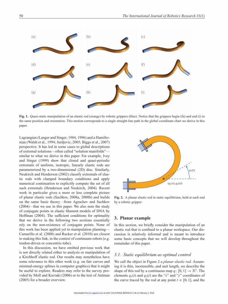
Fig. 1. Quasi-static manipulation of an elastic rod (orange) by robotic grippers (blue). Notice that the grippers begin (fa) and end (i) inthe same position and orientation. This motion corresponds to a single straight-line path in the global coordinate chart we derive in thispaper.

Lagrangian (Langer and Singer, 1984, 1996) and a Hamilto-nian (Walsh et al., 1994; Jurdjevic, 2005; Biggs et al., 2007)perspective. It has led in some cases to global descriptionsof extremal solutions—often called “solution manifolds”—similar to what we derive in this paper. For example, Iveyand Singer (1999) show that closed and quasi-periodicextremals of uniform, isotropic, linearly elastic rods areparameterized by a two-dimensional (2D) disc. Similarly,Neukirch and Henderson (2002) classify extremals of elas-tic rods with clamped boundary conditions and applynumerical continuation to explicitly compute the set of allsuch extremals (Henderson and Neukirch, 2004). Recentwork in particular gives a more or less complete pictureof planar elastic rods (Sachkov, 2008a, 2008b) and buildson the same basic theory—from Agrachev and Sachkov(2004)—that we use in this paper. We also note the studyof conjugate points in elastic filament models of DNA byHoffman (2004). The sufficient conditions for optimalitythat we derive in the following two sections essentiallyrely on the non-existence of conjugate points. None ofthis work has been applied yet to manipulation planning—Camarillo et al. (2008) and Rucker et al. (2010) are closestto making this link, in the context of continuum robots (e.g.tendon-driven or concentric-tube).

In this discussion, we have omitted previous work thatis not directly related either to analysis or manipulation ofa Kirchhoff elastic rod. Our results may nonetheless havesome relevance to this other work (e.g. on fair curves andminimal-energy splines in computer graphics) that it mightbe useful to explore. Readers may refer to the survey pro-vided by Moll and Kavraki (2006) or to the text of Antman(2005) for a broader overview.

(q1(t),q2(t))

q3(t)

Fig. 2. A planar elastic rod in static equilibrium, held at each endby a robotic gripper.

3. Planar example

In this section, we briefly consider the manipulation of anelastic rod that is confined to a planar workspace. Our dis-cussion is relatively informal and is meant to introducesome basic concepts that we will develop throughout theremainder of this paper.

3.1. Static equilibrium as optimal control

We call the object in Figure 2 a planar elastic rod. Assum-ing it is thin, inextensible, and unit length, we describe theshape of this rod by a continuous map q : [0, 1] → R

3. Theelements q1(t) and q2(t) are the “x” and “y” coordinates ofthe curve traced by the rod at any point t ∈ [0, 1], and the




element q3(t) is the tangent angle to this curve. We requirethe map q to satisfy

q1 = cos q3

q2 = sin q3

q3 = u

(1)

for some u : [0, 1] → R, which can be interpreted as strain(in bending). We refer to q and u together as (q, u). Weassume that the base of the rod is held fixed at the origin,so that q(0) = 0. The other end is held by a robotic grip-per, which we assume can impose arbitrary q(1) ∈ R

3. Forfixed q(1), the rod will remain motionless only if its shapelocally minimizes total elastic energy. In particular, we saythat (q, u) is in static equilibrium if it is a local optimum ofthe deterministic, continuous-time, optimal control problem

minimizeq,u

1

2

∫ 1

0u2dt

subject to q =⎡⎣cos q3

sin q3

u

⎤⎦q(0) = 0

q(1) = b

(2)

for some b ∈ R3. The cost function in equation (2) is a com-

monly used, first-order approximation to elastic energy thatis valid under the assumption of small deformations. Thisassumption requires only that the strain u(t) stays small, notthat changes in the configuration (q, u) are small. In partic-ular, the configuration shown in Figure 2 exhibits “smalldeformations” (as do the configurations in Figure 1 and,indeed, in all of the examples considered in this paper). Wealso note that although equilibrium configurations (q, u) arelocal optima of equation (2), there is nothing “local” aboutour model. Every possible equilibrium configuration is alocal optimum of equation (2) for some choice of b.

3.2. Quasi-static manipulation

Small changes b + δb in gripper placement will, in general,give rise to small changes (q + δq, u + δu) in a local opti-mum of equation (2), i.e. in an equilibrium configuration ofthe planar elastic rod. The problem of quasi-static manipu-lation planning is to find a continuous map β : [0, 1] → R

3

so that as s increases continuously from 0 to 1, there is alocal optimum of equation (2) with b = β(s) that changescontinuously from (qstart, ustart) to (qgoal, ugoal).

An immediate challenge in searching for β is that thegripper placement b does not uniquely define the configu-ration (q, u) of the rod. In general, equation (2) has manylocal optima for fixed b (e.g. see Figure 3), none of whichcan be computed in closed form. A similar challenge arisesin path planning for pick-and-place motions of an n-jointrobot arm, where there are (in general) many inverse kine-matic solutions for a given placement of the end-effector.There, we can avoid reasoning about the multiplicity of

inverse kinematic solutions by planning in the joint space

(e.g. S1 × n· · ·×S1) rather than in the task space (e.g. SE( 3)).We would like to apply this same approach to quasi-staticmanipulation, planning a path of the rod rather than of thegripper. However, it is not obvious how to describe the set ofall equilibrium configurations (i.e. the set of all local optimaof equation (2) over all possible b ∈ R

3), which is the natu-ral analog of “joint space” in this context. We show how todo this in the following section.

3.3. Analysis of equilibrium configurations

Considerable insight can be obtained by applying the max-imum principle of Pontryagin et al. (1962) to the optimalcontrol problem equation (2). If

(q, u) : [0, 1] → R3 × R

is a local optimum of equation (2), then the maximumprinciple tells us that there must exist a co-state trajectory

p : [0, 1] → R3

and a constant k ≥ 0, not both zero, that satisfy

q = ∇pH( p, q, k, u)T

p = −∇qH( p, q, k, u)T(3)

and

H (p(t) , q(t) , k, u(t) ) = maxv

H (p(t) , q(t) , k, v) (4)

for all t ∈ [0, 1], where

H( p, q, k, u) = p1 cos q3 + p2 sin q3 + p3u − k1

2u2

is the Hamiltonian function associated with equation (2).When applying these necessary conditions, we often dis-

tinguish between the abnormal case in which k = 0, and thenormal case in which k > 0, where as usual we may simplyassume that k = 1 (see, for example, Souéres and Boisson-nat (1998)). Taking the abnormal case first, the conditionsin equations (3) and (4) require that

q1 = cos q3 p1 = 0

q2 = sin q3 p2 = 0

q3 = u p3 = p1 sin q3 − p2 cos q3

(5)

and

0 = p3,

respectively. Since p1, p2, and

p1 sin q3 − p2 cos q3

are evidently all constant, it must be the case that q3 is alsoconstant. We conclude that (q, u) is “abnormal” if and onlyif u(t) = 0 for all t ∈ [0, 1], i.e. if and only if the rod




Fig. 3. Quasi-static manipulation of a planar elastic rod. Notice that the grippers begin and end in the same position and orientation–gripper placement does not uniquely define the configuration of the rod.

is straight. Turning now to the normal case, equation (3)requires equation (5) just as before, while equation (4) nowrequires that

u = p3. (6)

From equations (5) and (6), we see that “normal” (q, u) andp are completely defined by p(0), the choice of initial co-state. It is also easy to verify that

u(t) = 0 for all t ∈ [0, 1] ⇐⇒ p2(0) = p3(0) = 0,

so every abnormal (q, u) is also normal. As a consequence,every possible equilibrium configuration of the planar elas-tic rod can be generated by an appropriate choice of p(0) ∈R

3. In particular, the set of all equilibrium configurations—analogous to the “joint space” for an n-joint robot arm—isapparently a subset of R

3. This result is already somewhatremarkable, given that arbitrary configurations (q, u) live ina space of infinite dimension.

3.4. Physical interpretation of the co-statetrajectory

The co-state trajectory p : [0, 1] → R3 that is produced

by application of the maximum principle has a physicalinterpretation. To provide this interpretation, we begin byassuming that p(t) describes the force and torque acting onthe rod at t ∈ [0, 1], and proceed to check if this assumptionallows us to reconstruct the governing equations equation(5) and equation (6). In particular, consider a small pieceof the planar elastic rod, as shown in Figure 4(a). In staticequilibrium, a force and torque balance requires that

p1(t + �t) −p1(t) = 0

p2(t + �t) −p2(t) = 0

p3(t + �t) −p3(t) = p1(t + �t) (q2(t + �t) −q2(t))

− p2(t + �t) (q1(t + �t) −q1(t)) .

In the limit as �t → 0, we recover

p1 = 0

p2 = 0

p3 = p1q2 − p2q1 = p1 sin q3 − p2 cos q3,

(7)

exactly as in equation (5). Equation (6) follows immediatelyfrom the linear relationship between stress and strain. Weconclude that p(t) does indeed describe force and torque,and specifically that every equilibrium configuration iscompletely defined by the force and torque at the base ofthe rod (i.e. by p(0)). It is even possible to show that (q, u)is abnormal if and only if p(0) is indeterminate, a result thatwill be useful to us in characterizing degeneracies of themapping from b + δb to (q + δq, u + δu).

Before proceeding, we consider the same force andtorque balance in a local reference frame, as in Figure 4(b).Define μ : [0, 1] → R

3 as⎡⎣μ1(t)μ2(t)μ3(t)

⎤⎦ =⎡⎣ cos q3(t) sin q3(t) 0

− sin q3(t) cos q3(t) 00 0 1

⎤⎦⎡⎣p1(t)p2(t)p3(t)

⎤⎦for all t ∈ [0, 1]. Either by applying this transform to equa-tion (7) or by taking a force and torque balance, we findthat

μ1 = μ2μ3

μ2 = −μ1μ3

μ3 = −μ2,

(8)

where u = μ3. Equations (7) and (8) are equivalent—anyequilibrium configuration can be generated either by spec-ifying p(0) or by specifying μ(0). However, it is interest-ing to note that equation (8)—unlike equation (7)—has nodependence on q. This sort of “reduction” will become veryimportant as we generalize our approach to a geometricsetting.

Finally, notice that the signed curvature of the curve(q1, q2) : [0, 1] → R

2 that is traced by the planar elasticrod is given by κ = u = μ3. It is easy to verify that

2κ + κ3 = λκ (9)

and equation (8) are equivalent, where

λ = μ3(0)2 +2μ1(0)

is a constant of integration. In this way, we recover thevariational constraint in equation (9) that would have beenproduced by analysis of equation (2) from a Lagrangianperspective (as in Langer and Singer (1984, 1996)).




(a)

p1(t)

p2(t)

p3(t)

p1(t +Δ t)

p2(t +Δ t)

p3(t +Δ t)

(b)

µ1(t)

µ2(t)

µ3(t)

µ1(t +Δ t)

µ2(t +Δ t)

µ3(t +Δ t)

Fig. 4. Forces and torques applied to a piece of the planar elastic rod (a) in a global reference frame and (b) in a local reference frame,providing a physical interpretation of the co-state trajectory.

3.5. Outline

In the rest of this paper, we make precise the ideas discussedabove and generalize them to enable quasi-static manipula-tion of an elastic rod in a 3D workspace. A key differencein what follows is that the rod’s shape will be described byq : [0, 1] → S E( 3) instead of q : [0, 1] → R

3, and conse-quently that equation (2) will become a problem of optimalcontrol on manifolds. To obtain the necessary conditionsfor optimality that are analogous to what appeared in Sec-tion 3.3, we will be forced on rely on a geometric statementof Pontryagin’s maximum principle. We provide these nec-essary conditions—as well as sufficient conditions, whichwere completely ignored in the above discussion and whichare considerably more involved—in Section refsec:theory.We apply them to study the mechanics of the elasticrod in Section 5, and to study manipulation of this rod inSection 6.

4. Theoretical framework

We will see in Section 5 that the framed curve traced byan elastic rod in static equilibrium is a local solution to ageometric optimal control problem. Here, we provide theframework to characterize this solution. This frameworkessentially relies on a geometric statement of Pontryagin’smaximum principle (Pontryagin et al., 1962). Section 4.1reviews smooth manifolds and is included to fix notation.Section 4.2 states the necessary and sufficient conditionsfor optimality on manifolds in a form that is useful for us.Section 4.3 derives coordinate formulae to compute thesenecessary and sufficient conditions. Most of these resultsare a translation of Agrachev and Sachkov (2004) in a stylemore consistent with Marsden and Ratiu (1999) and Lee(2003). We conclude with coordinate formulae to test suf-ficiency for left-invariant systems on Lie groups (Theorem4), an important result that is not in Agrachev and Sachkov(2004) and that is hard to find elsewhere.

4.1. Smooth manifolds

In this section, we review some basic facts about smoothmanifolds. We do so mainly to establish notation for whatfollows.

Let M be a smooth manifold. The space of all smoothreal-valued functions on M is C∞( M). The space of allsmooth vector fields on M is X( M). The action of a tan-gent vector v ∈ TmM on a function f ∈ C∞( M) is v · f .The action of a tangent covector w ∈ T∗

mM on a tangentvector v ∈ TmM is 〈w, v〉. The action of a vector fieldX ∈ X( M) on a function f ∈ C∞( M) produces the functionX [f ] ∈ C∞( M) that satisfies

X [f ]( m) = X ( m) ·ffor all m ∈ M . The Jacobi–Lie bracket of vector fieldsX , Y ∈ X( M) is the vector field [X , Y ] ∈ X( M) thatsatisfies

[X , Y ][f ] = X [Y [f ]] − Y [X [f ]]

for all f ∈ C∞(M). If F : M → N is a smooth map betweensmooth manifolds M and N , then the pushforward of Fat m ∈ M is the linear map TmF : TmM → TF(m)N thatsatisfies

TmF( v) ·f = v · (f ◦ F)

for all v ∈ TmM and f ∈ C∞( N). The pullback of F atm ∈ M is the dual map T∗

mF : T∗F(m)N → T∗

mM that satisfies⟨T∗

mF( w) , v⟩ = 〈w, TmF( v) 〉

for all v ∈ TmM and w ∈ T∗F(m)N . We say F is degener-

ate at m ∈ M if there exists non-zero v ∈ TmM such thatTmF( v) = 0. It is equivalent that the Jacobian matrix of anycoordinate representation of F at m has zero determinant.The Poisson bracket generated by the canonical symplecticform on T∗M is

{·, ·} : C∞( T∗M) ×C∞( T∗M) → C∞( T∗M) .

The co-tangent bundle T∗M together with the bracket {·, ·}is a Poisson manifold. The Hamiltonian vector field of H ∈C∞( T∗M) is the unique vector field XH ∈ X( T∗M) thatsatisfies

XH [K] = {K, H}

for all K ∈ C∞( T∗M). It is equivalent to say that H isa Hamiltonian function for the vector field XH . We usethis same notation when H (hence, XH ) is time-varying.Finally, we use π : T∗M → M to denote the projection mapsatisfying π ( w, m) = m for all w ∈ T∗

mM . at UNIV CALIFORNIA BERKELEY LIB on February 3, 2016ijr.sagepub.comDownloaded from



4.2. Optimal control on manifolds

In this section, we state the necessary and sufficient con-ditions for optimal control problems on smooth manifolds.These conditions are analogous to what is provided by Pon-tryagin’s maximum principle, which is usually applied tooptimal control problems on Euclidean space.

Let U ⊂ Rm for some m > 0. Assume g : M × U →

R and f : M × U → TM are smooth maps. Consider theoptimal control problem

minimizeq,u

∫ 1

0g (q(t) , u(t) ) dt

subject to q(t) = f (q(t) , u(t) ) for all t ∈ [0, 1]

q(0) = q0, q(1) = q1,

(10)

where q0, q1 ∈ M and (q, u) : [0, 1] → M × U .Define the parameterized Hamiltonian functionH : T∗M × R × U → R by

H( p, q, k, u) = 〈p, f (q, u) 〉 − kg(q, u) ,

where p ∈ T�q M . The following theorem is a geometric

statement of Pontryagin’s maximum principle (Pontryaginet al., 1962):

Theorem 1 (Necessary conditions). Suppose (qopt, uopt) :[0, 1] → M × U is a local optimum of equation (10). Then,there exists k ≥ 0 and an integral curve ( p, q) : [0, 1] →T∗M of the time-varying Hamiltonian vector field XH ,where H : T∗M × R → R is given by H( p, q, t) =H( p, q, k, uopt(t)), that satisfies q(t) = qopt(t) and

H( p(t) , q(t) , t) = maxu∈U

H( p(t) , q(t) , k, u) (11)

for all t ∈ [0, 1]. Furthermore, if k = 0, then p(t) �= 0 forall t ∈ [0, 1].

Proof. See Theorem 12.10 of Agrachev and Sachkov(2004).

We call the integral curve ( p, q) in Theorem 1 an abnor-mal extremal when k = 0 and a normal extremal otherwise.As usual, when k �= 0 we may simply assume k = 1. Wecall (q, u) abnormal if it is the projection of an abnormalextremal. We call (q, u) normal if it is the projection of anormal extremal and it is not abnormal.

Theorem 2 (Sufficient conditions). Suppose ( p, q) : [0, 1]→ T∗M is a normal extremal of equation (10). Define H ∈C∞( T∗M) by

H( p, q) = maxu∈U

H( p, q, 1, u) , (12)

assuming the maximum exists and ∂2H/∂u2 < 0. Defineu : [0, 1] → U so u(t) is the unique maximizer of equation(12) at ( p(t) , q(t)). Assume that XH is complete and thatthere exists no other integral curve ( p′, q′) of XH satisfyingq(t) = q′(t) for all t ∈ [0, 1]. Let ϕ : R × T∗M → T∗M be

the flow of XH and define the endpoint map φt : T∗q(0)M → M

by φt( w) = π ◦ϕ(t, w, q(0)). Then, (q, u) is a local optimumof equation (10) if and only if there exists no t ∈(0, 1] forwhich φt is degenerate at p(0).

Proof. See Theorem 21.8 of Agrachev and Sachkov (2004).

4.3. Lie–Poisson reduction

The necessary and sufficient conditions provided by Theo-rems 1 and 2 are, in principle, all we need to characterizesolutions to optimal control problems on manifolds. How-ever, it is not apparent yet how to compute anything—inparticular, how to compute integral curves ( p, q) or to estab-lish non-degeneracy of the endpoint map φt. In this section,we apply the Lie–Poisson reduction to provide coordinateformulae for computation in the specific case where themanifold is a Lie Group and the Hamiltonian function isleft-invariant. As we will see in Section 5, this case issatisfied by a Kirchhoff elastic rod.

First, we establish some additional notation. Let G be aLie group with identity element e ∈ G. Let g = TeG andg∗ = T∗

e G. For any q ∈ G, define the left translation mapLq : G → G by

Lq( r) = qr

for all r ∈ G. A function H ∈ C∞( T∗G) is left-invariant if

H(T∗

r Lq( w) , r) = H( w, s)

for all w ∈ T∗s G and q, r, s ∈ G satisfying s = Lq( r). For

any ζ ∈ g, let Xζ be the vector field that satisfies

Xζ (q) = TeLq( ζ )

for all q ∈ G. Define the Lie bracket [·, ·] : g × g → g by

[ζ , η] = [Xζ , Xη

]( e)

for all ζ , η ∈ g. For any ζ ∈ g, the adjoint operatoradζ : g → g satisfies

adζ ( η) = [ζ , η]

and the co-adjoint operator ad∗ζ : g∗ → g∗ satisfies⟨

ad∗ζ ( μ) , η

⟩ = ⟨μ, adζ η

⟩for all η ∈ g and μ ∈ g∗. The functional derivative of h ∈C∞( g∗) at μ ∈ g∗ is the unique element δh/δμ of g thatsatisfies

lims→0

h (μ + sδμ) − h (μ)

s=⟨δμ,

δh

δμ

⟩for all δμ ∈ g∗.

Next, we revisit our statement of necessary conditions forthe optimal control problem equation (10) in the case whereM = G and where the Hamiltonian H is left-invariant. The-orem 1 implies the existence of a particular integral curve




( p, q) in the cotangent bundle T∗G. The following theoremimplies the existence of a corresponding integral curve μ

in the dual Lie algebra g∗. This result is important becauseg∗ is a vector space and so μ can be readily computed bysolving a system of ordinary differential equations, as wewill see in Theorem 4 (to follow).

Theorem 3 (Reduction of necessary conditions). Supposethe time-varying Hamiltonian function H : T∗G × [0, 1] →R is both smooth and left-invariant for all t ∈ [0, 1]. Denotethe restriction of H to g∗ by h = H |g∗×[0,1]. Given p0 ∈T∗

q0G, let μ : [0, 1] → g∗ be the solution of

μ = ad∗δh/δμ( μ) (13)

with initial condition μ(0) = T∗e Lq0 ( p0). The integral curve

( p, q) : [0, 1] → T∗G of XH with initial condition p(0) = p0

satisfiesp(t) = T∗

q(t)Lq(t)−1 (μ(t) )

for all t ∈ [0, 1], where q is the solution of

q = Xδh/δμ(q)

with initial condition q(0) = q0.

Proof. See Theorem 13.4.4 of Marsden and Ratiu (1999).

In what follows, it will be convenient for us to introducecoordinates on g and g∗. Let {X1, . . . , Xn} be a basis for gand let {P1, . . . , Pn} be the dual basis for g∗ that satisfies⟨

Pi, Xj

⟩ = δij,

for i, j ∈ {1, . . . , n}, where δij is the Kronecker delta. Wewrite ζi to denote the ith component of ζ ∈ g with respectto this basis, and so forth. Define the structure constantsCk

ij ∈ R associated with our choice of basis by

[Xi, Xj] =n∑

k=1

CkijXk (14)

for i, j ∈ {1, . . . , n}.Finally, we revisit our statement of sufficient conditions

for equation (10), and provide coordinate formulae to testthe non-degeneracy of the endpoint map φt that was definedin Theorem 2. These formulae can be evaluated by solvinga system of linear, time-varying matrix differential equa-tions, something that is easy to do using modern numericalmethods. We require two lemmas before our main result inTheorem 4:

Lemma 1. Let q : U → G be a smooth map, where U ⊂ R2

is simply connected. Denote its partial derivatives ζ : U →g and η : U → g by

ζ (t, ε) = Tq(t,ε)Lq(t,ε)−1

(∂q(t, ε)

∂t

)η(t, ε) = Tq(t,ε)Lq(t,ε)−1

(∂q(t, ε)

∂ε

).

(15)

Then,∂ζ

∂ε− ∂η

∂t= [ζ , η]. (16)

Conversely, if there exists smooth maps ζ and η satisfyingequation (16), then there exists a smooth map q satisfyingequation (15).

Proof. See Proposition 5.1 of Bloch et al. (1996).

Lemma 2. Let α, β, γ ∈ g and suppose γ = [α, β]. Then

γk =n∑

r=1

n∑s=1

αrβsCkrs.

Proof. This result is easily obtained from the definition inequation (14).

Theorem 4 (Reduction of sufficient conditions). Supposethat H ∈ C∞( T∗G) is left-invariant and that XH is com-plete. Let h = H |g∗ be the restriction of H to g∗ andlet ϕ : R × T∗G → T∗G be the flow of XH . Given q0 ∈G, define the endpoint map φt : T∗

q0G → G by φt( p) =

π◦ϕ(t, p, q0). Given p0 ∈ T∗q0

G, let a ∈ Rn be the coordinate

representation of T∗e Lq0 ( p0), i.e.

T∗e Lq0 ( p0) =

n∑i=1

aiPi. (17)

Solve the ordinary differential equations

μi = −n∑

j=1

n∑k=1

Ckij

δh

δμjμk i ∈ {1, . . . , n} (18)

with the initial conditions μi(0) = ai for i ∈ {1, . . . , n}.Define matrices F, G, H ∈ R

n×n as follows:

[F]ij = − ∂

∂μj

n∑r=1

n∑s=1

Csir

δh

δμrμs

[G]ij = ∂

∂μj

δh

δμi

[H]ij = −n∑

r=1

δh

δμrCi

rj.

Solve the (linear, time-varying) matrix differential equa-tions

M = FM (19)

J = GM + HJ (20)

with initial conditions M(0) = I and J(0) = 0. Theendpoint map φt is degenerate at p0 if and only ifdet (J(t) ) = 0.

Proof. Define the smooth map ρ : Rn → T∗

q0G by

ρ( a) = T∗q0

L−1q0

(n∑

i=1

aiPi

).




This same expression defines ρ : Rn → Tp0 (T∗

q0G) if we

identify T∗q0

G with Tp0 (T∗q0

G) in the usual way. Given p0 =ρ( a) for some a ∈ R

n, there exists non-zero λ ∈ Tp0 (T∗q0

G)satisfying Tp0φt( λ) = 0 if and only if there exists non-zeros ∈ R

n satisfying Tρ(a)φt( ρ(s)) = 0. Define the smooth mapq : [0, 1] × R

n → G by q(t, a) = φt ◦ ρ( a). Noting that

∂q(t, a)

∂aj= Tρ(a)φt

(T∗

q0Lq−1

0( Pj)

)for j ∈ {1, . . . , n}, we have

Tρ(a)φt( ρ(s)) =n∑

j=1

sj∂q(t, a)

∂aj.

By left translation, Tρ(a)φt( ρ(s)) = 0 if and only if

0 =n∑

j=1

sjTq(t,a)Lq(t,a)−1

(∂q(t, a)

∂aj

). (21)

For each j ∈ {1, . . . , n}, let

ηj(t, a) = Tq(t,a)Lq(t,a)−1

(∂q(t, a)

∂aj

).

Define J : [0, 1] → Rn×n so that J(t) has entries

[J]ij = ηji(t, a) ,

i.e. the jth column of J(t) is the coordinate representationof ηj(t, a) with respect to {X1, . . . , Xn}. Then, equation (21)holds for some s �= 0 if and only if det (J(t) ) = 0. Weconclude that φt is degenerate at p0 if and only ifdet (J(t) ) = 0.

It remains to show that J(t) can be computed as describedin the theorem. Taking μ1(t) , . . . , μn(t) as coordinates ofμ(t), it is easy to verify that equations (13) and (18) areequivalent (see Marsden and Ratiu (1999)). We extend eachcoordinate function in the obvious way to μi : [0, 1]×R

n →R, so μi(t, a) solves equation (18) with initial conditionμi(0, a) = ai. Define M : [0, 1] → R

n×n by

[M(t) ]ij = ∂μi/∂aj.

Differentiating equation (18), we compute

[M]ij = ∂

∂t

∂μi

∂aj= ∂

∂aj

∂μi

∂t= ∂

∂aj

(−

n∑r=1

n∑s=1

Csir

δh

δμrμs

)

=n∑

k=1

− ∂

∂μk

(n∑

r=1

n∑s=1

Csir

δh

δμrμs

)∂μk

∂aj

=n∑

k=1

[F]ik[M]kj.

It is clear that [M(0) ]ij = δij, so we have verified equation(19). Next, define

ζ (t, a) = Tq(t,a)Lq(t,a)−1

(∂q(t, a)

∂t

).

We have

ηj = ∂ζ

∂aj− [

ζ , ηj] = ∂

∂aj

δh

δμ−[

δh

δμ, ηj

]

from Lemma 1 and Theorem 3. We write this equation incoordinates by application of Lemma 2:

[J]ij = ηji =

n∑k=1

(∂

∂μk

δh

δμi

)∂μk

∂aj+

n∑k=1

(−

n∑r=1

δh

δμrCi

rk

)η

jk

=n∑

k=1

[G]ik[M]kj +n∑

k=1

[H]ik[J]kj.

It is clear that [J(0) ]ij = 0, so we have verified equation(20).

5. Mechanics of an elastic rod

The previous section derived coordinate formulae to com-pute necessary and sufficient conditions for a particularclass of optimal control problems on manifolds. Here, weapply these formulae to a Kirchhoff elastic rod.

We begin with three results that suffice to describe allpossible configurations of the rod that can be achievedby quasi-static manipulation. Section 5.1 recalls that anyframed curve traced by the rod in static equilibrium canbe described as a local solution to a geometric optimalcontrol problem (Walsh et al., 1994; Biggs et al., 2007).Section 5.2 proves that the set of all trajectories that arenormal with respect to this problem is a smooth man-ifold of finite dimension that can be parameterized bya single chart (Theorem 6). Section 5.3 proves that theset of all normal trajectories that are also local optimais an open subset of this smooth manifold, and pro-vides a computational test for membership in this subset(Theorem 7).

We conclude with two additional results that, as we willsee in Section 6, are useful in the context of a sampling-based planning algorithm for manipulation planning. Sec-tion 5.4 provides a physical interpretation of the coordinatechart we derive as a space of moments and forces. Sec-tion 5.5 defines a “straight-line path” in both this chart andin the space of boundary conditions.

5.1. Model

We refer to the object in Figure 1 as a rod. Assuming thatit is thin, inextensible, and of unit length, we describe theshape of this rod by a continuous map q : [0, 1] → G, whereG = SE( 3). Abbreviating TeLq( ζ ) = qζ as usual for matrixLie groups, we require this map to satisfy

q = q( u1X1 + u2X2 + u3X3 + X4) (22)




for some u : [0, 1] → U , where U = R3 and

X1 =

⎡⎢⎢⎣0 0 0 00 0 −1 00 1 0 00 0 0 0

⎤⎥⎥⎦X2 =

⎡⎢⎢⎣0 0 1 00 0 0 0

−1 0 0 00 0 0 0

⎤⎥⎥⎦X3 =

⎡⎢⎢⎣0 −1 0 01 0 0 00 0 0 00 0 0 0

⎤⎥⎥⎦

X4 =

⎡⎢⎢⎣0 0 0 10 0 0 00 0 0 00 0 0 0

⎤⎥⎥⎦X5 =

⎡⎢⎢⎣0 0 0 00 0 0 10 0 0 00 0 0 0

⎤⎥⎥⎦X6 =

⎡⎢⎢⎣0 0 0 00 0 0 00 0 0 10 0 0 0

⎤⎥⎥⎦is a basis for g. Denote the dual basis for g∗ by {P1, . . . , P6}.We refer to q and u together as (q, u) : [0, 1] → G × U orsimply as (q, u). Each end of the rod is held by a roboticgripper. We ignore the structure of these grippers, and sim-ply assume that they fix arbitrary q(0) and q(1). We furtherassume, without loss of generality, that q(0) = e. We denotethe space of all possible q(1) by B = G. Finally, we assumethat the rod is elastic in the sense of Kirchhoff (Biggs et al.,2007), so has total elastic energy

1

2

∫ 1

0

(c1u2

1 + c2u22 + c3u2

3

)dt

for given constants c1, c2, c3 > 0. For fixed endpoints, therod will be motionless only if its shape locally minimizesthe total elastic energy. In particular, we say that (q, u) is instatic equilibrium if it is a local optimum of

minimizeq,u

1

2

∫ 1

0

(c1u2

1 + c2u22 + c3u2

3

)dt

subject to q = q( u1X1 + u2X2 + u3X3 + X4)

q(0) = e, q(1) = b

(23)

for some b ∈ B.

5.2. Necessary conditions for static equilibrium

We have seen that if a Kirchhoff elastic rod is in staticequilibrium, then its configuration (q, u) must be a localsolution to the geometric optimal control problem in equa-tion (23). In this section, we apply the necessary conditionsfor optimality to show that the set of all normal (q, u) is asmooth 6-manifold that can be parameterized by a singlechart. Coordinates for this chart are given by the open sub-set A ⊂ R

6 that is defined by equation (27) in the followingtheorem. Our main result is then Theorem 6.

Theorem 5. A trajectory (q, u) is normal with respect toequation (23) if and only if there exists μ : [0, 1] → g∗ thatsatisfies

μ1 = u3μ2 − u2μ3 μ4 = u3μ5 − u2μ6

μ2 = μ6 + u1μ3 − u3μ1 μ5 = u1μ6 − u3μ4 (24)

μ3 = −μ5 + u2μ1 − u1μ2 μ6 = u2μ4 − u1μ5,

q = q( u1X1 + u2X2 + u3X3 + X4) , (25)

ui = c−1i μi for all i ∈ {1, 2, 3}, (26)

with initial conditions q(0) = e and μ(0) = ∑6i=1 aiPi for

some a ∈ A, where

A = {a ∈ R

6 : ( a2, a3, a5, a6) �=(0, 0, 0, 0)}

. (27)

Proof. We begin by showing that (q, u) is abnormal if andonly if u2 = u3 = 0. Theorem 1 tells us that (q, u) is abnor-mal if and only if it is the projection of an integral curve( p, q) of XH that satisfies equation (11), where

H( p, q, t) = H( p, q, 0, u(t))

and

H( p, q, 0, u) = 〈p, q( u1X1 + u2X2 + u3X3 + X4) 〉 .

For any g, r ∈ G satisfying q = gr, we compute

H(T∗r Lg( p) , r, t)

= ⟨T∗

r Lg( p) , g−1q( u1X1 + u2X2 + u3X3 + X4)⟩

= ⟨p, g

(g−1q( u1X1 + u2X2 + u3X3 + X4)

)⟩(28)

= 〈p, q( u1X1 + u2X2 + u3X3 + X4) 〉= H( p, q, t) ,

so H is left-invariant. As a consequence, the existence of( p, q) satisfying the conditions of Theorem 1 is equivalentto the existence of μ satisfying the conditions of Theorem 3:

μ = ad∗δh/δμ( μ) and q = q( δh/δμ) ,

where h = H |g∗ . Application of equation (18) produces theformulae in equations (24)–(25), where we require μ1 =μ2 = μ3 = 0 to satisfy equation (11). We therefore haveμ2 = μ6 and μ3 = −μ5, hence μ5 = μ6 = 0. Applyingthis result again to equation (24), we find μ5 = −u3μ4 = 0and μ6 = u2μ4 = 0. Since μ cannot vanish when k = 0, wemust have μ4 �= 0, hence u2 = u3 = 0, with u1 an arbitraryintegrable function. Our result follows.

Now, we return to the normal case. As before, Theorem 1tells us that (q, u) is normal if and only if it is not abnormaland it is the projection of an integral curve ( p, q) of XH thatsatisfies equation (11), where

H( p, q, t) = H( p, q, 1, u(t))

and

H( p, q, 1, u) = 〈p, q( u1X1 + u2X2 + u3X3 + X4) 〉− (

c1u21 + c2u2

2 + c3u23

)/2.

By a computation identical to equation (28), H is left-invariant. Application of equation (18) to the conditionsof Theorem 3 produces the same formulae in equations(24)–(25), where equation (26) follows from equation (11)because H is quadratic in u. It remains to show that trajec-tories produced by equations (24)–(26) are not abnormal ifand only if a ∈ A. We prove the converse. First, assumea ∈ R

6\A, so ( a2, a3, a5, a6) =(0, 0, 0, 0). From equations




(24) and (26), we see that u2 = u3 = 0, hence (q, u) isabnormal. Now, assume (q, u) is abnormal, so u2 = u3 = 0.From equation (26), we therefore have μ2 = μ3 = 0, and inparticular a2 = a3 = 0. Plugging this result into equation(24), we see that μ2 = μ6 and μ3 = −μ5, hence also thatμ5 = μ6 = 0, i.e. that a5 = a6 = 0. So, a ∈ R

6\A. Ourresult follows.

Theorem 5 provides a set of candidates for local optimaof equation (23), which we now characterize. Denote theset of all smooth maps (q, u) : [0, 1] → G × U under thesmooth topology2 by C∞( [0, 1], G × U). Let

C ⊂ C∞( [0, 1], G × U)

be the subset of all (q, u) that satisfy Theorem 5. Any such(q, u) ∈ C is completely defined by the choice of a ∈ A, asis the corresponding μ. Denote the resulting maps by

�( a) =(q, u) �( a) = μ.

We require three lemmas before our main result inTheorem 6.

Lemma 3. If �( a) = �( a′) for some a, a′ ∈ A, thena = a′.

Proof. Suppose (q, u) = �( a) and μ = �( a) for some a ∈A. It suffices to show that a is uniquely defined by u (and itsderivatives, since u is clearly smooth). From equation (26),we have

a1 = c1u1(0)

a2 = c2u2(0)

a3 = c3u3(0) .

(29)

From equation (24), we have

a5 = −c3u3(0) +a1a2( c−12 − c−1

1 )

a6 = c2u2(0) −a1a3( c−11 − c−1

3 ) .(30)

It is now possible to compute μi(0) and μi(0) for i ∈{4, 5, 6} by differentiation of

μ4 = u3μ5 − u2μ6

μ5 = −μ3 + u2μ1 − u1μ2

μ6 = μ2 − u1μ3 − u3μ1,

(31)

where we use equation (26) to find derivatives of μi(0)for i ∈ {1, 2, 3}. Based on these results, we differentiateequation (24) again to produce

( c−13 a3) a4 = c−1

1 a1a6 − μ5(0)

( c−12 a2) a4 = c−1

1 a1a5 + μ6(0)

( −a5 + a1a2( c−12 − c−1

1 )) a4 = c3( c−11 ( μ1(0) a6

+ a1μ6(0)) −μ5(0)) −a3μ4(0) (32)

( a6 + a1a3( c−11 − c−1

3 ) a4 = c2( c−11 ( μ1(0) a5

+ a1μ5(0)) +μ6(0)) −a2μ4(0) .

At least one of these four equations allows us to compute a4

unless( a2, a3, a5, a6) =(0, 0, 0, 0) ,

which would violate our assumption that a ∈ A. Our resultfollows.

Lemma 4. The map � : A → C is a homeomorphism.

Proof. The map � is clearly a bijection—it is well-definedand onto by construction, and is one-to-one by Lemma 3.Continuity of � also follows immediately from Theorem 5.

It remains only to show that �−1 : C → A iscontinuous. This result is a corollary to the proof ofLemma 3. From equation (29), we see that a1, a2, a3 dependcontinuously on u(0). From equation (30), we see thata5, a6 depend continuously on a1, a2, a3, u(0), hence onu(0) , u(0). From equation (31), we see in the same way thatμ4(0) , μ5(0) , μ6(0) , μ5(0) , μ6(0) depend continuously onu(0) , u(0) , u(0). Hence, all of the quantities in equation (32)depend continuously on u(0) , u(0) , u(0), so a4 does as well.Our result follows.

Lemma 5. If the topological n-manifold M has an atlasconsisting of the single chart (M , α), then N = α(M) is atopological n-manifold with an atlas consisting of the singlechart (N , idN ), where idN is the identity map. Furthermore,both M and N are smooth n-manifolds and α : M → N is adiffeomorphism.

Proof. Since (M , α) is a chart, then N is an open subset ofR

n and α is a bijection. Hence, our first result is immedi-ate and our second result requires only that both α and α−1

are smooth maps. For every p ∈ M , the charts (M , α) and(N , idN ) satisfy α( p) ∈ N , α(M) = N , and idN ◦ α ◦ α−1 =idN , so α is a smooth map. For every q ∈ N , the charts(N , idN ) and (M , α) again satisfy α−1(q) ∈ M , α−1(N) = M ,and α ◦ α−1 ◦ idN = idN , so α−1 is also a smooth map. Ourresult follows.

Theorem 6. C is a smooth 6-manifold with smooth struc-ture determined by an atlas with the single chart ( C, �−1).

Proof. Since � : A → C is a homeomorphism by Lemma 4and A ⊂ R

6 is open, then ( C, �−1) is a chart whose domainis C. Our result follows from Lemma 5.

5.3. Sufficient conditions for static equilibrium

As we have seen, any trajectory (q, u) that is normal withrespect to the optimal control problem equation (23) can berepresented in coordinates by a point a ∈ A. In this section,we show that any such point a produces a local optimum�( a) of equation (23) if and only if it is an element of aparticular open subset Astable ⊂ A. In particular, the follow-ing theorem provides a computational test for membershipin this subset:

Theorem 7. Let (q, u) = �( a) and μ = �( a) for somea ∈ A. Define at UNIV CALIFORNIA BERKELEY LIB on February 3, 2016ijr.sagepub.comDownloaded from



F =

⎡⎢⎢⎢⎢⎢⎢⎣0 μ3( c−1

3 − c−12 ) μ2( c−1

3 − c−12 ) 0 0 0

μ3( c−11 − c−1

3 ) 0 μ1( c−11 − c−1

3 ) 0 0 1μ2( c−1

2 − c−11 ) μ1( c−1

2 − c−11 ) 0 0 −1 0

0 −μ6/c2 μ5/c3 0 μ3/c3 −μ2/c2

μ6/c1 0 −μ4/c3 −μ3/c3 0 μ1/c1

−μ5/c1 μ4/c2 0 μ2/c2 −μ1/c1 0

⎤⎥⎥⎥⎥⎥⎥⎦G = diag

(c−1

1 , c−12 , c−1

3 , 0, 0, 0)

H =

⎡⎢⎢⎢⎢⎢⎢⎣0 μ3/c3 −μ2/c2 0 0 0

−μ3/c3 0 μ1/c1 0 0 0μ2/c2 −μ1/c1 0 0 0 0

0 0 0 0 μ3/c3 −μ2/c2

0 0 1 −μ3/c3 0 μ1/c1

0 −1 0 μ2/c2 −μ1/c1 0

⎤⎥⎥⎥⎥⎥⎥⎦ .

Solve the (linear, time-varying) matrix differentialequations

M = FM

J = GM + HJ(33)

with initial conditions M(0) = I and J(0) = 0. Then, (q, u)is a local optimum of equation (23) for b = q(1) if and onlyif det( J(t)) �= 0 for all t ∈(0, 1].

Proof. As we have already seen, normal extremals of equa-tion (23) are derived from the parameterized Hamiltonianfunction

H( p, q, 1, u) = 〈p, q( u1X1 + u2X2 + u3X3 + X4) 〉−1

2

(c1u2

1 + c2u22 + c3u2

3

).

This function satisfies

∂2H

∂u2= − diag( c1, c2, c3) < 0

and admits a unique maximum at

ui = c−1i 〈p, qXi〉

for i ∈ {1, 2, 3}. The maximized Hamiltonian function is

H( p, q) = 1

2

3∑i=1

c−1i 〈p, qXi〉2 + 〈p, qX4〉 .

It is clear that XH is complete. By Lemma 3, the mappingfrom (q, u) to a and hence to μ = �( a) is unique. ByTheorem 3, it is equivalent that the mapping from (q, u) to( p, q) is unique. As a consequence, we may apply Theo-rem 2 to establish sufficient conditions for optimality. Sincea computation identical to equation (28) shows that H isleft-invariant, we may apply the equivalent conditions of

Theorem 4. Noting that the restriction h = H |g∗ ∈ C∞( g∗)is given by

h( μ) = 1

2

(μ2

1

c1+ μ2

2

c2+ μ2

3

c3

)+ μ4,

it is easy to verify that F, G and H take the form givenabove. Our result follows.

As we have said, Theorem 7 provides a computationaltest of which points a ∈ A actually produce local optima�( a) ∈ C of equation (23). Let

Astable ⊂ Abe the subset of all a for which the conditions of Theorem7 are satisfied and let

Cstable = �(Astable) ⊂ C.

An important consequence of membership in Astable issmooth local dependence of solutions to equation (23) onvariation in b. Define

Bstable = {b ∈ B : there exists (q, u) ∈ Cstable

for which q(1) = b}.

Let � : C → B be the map taking (q, u) to q(1). ClearlyAstable is open, so

�|Astable : Astable → Cstable

is a diffeomorphism. We arrive at the following result:

Theorem 8. The map

� ◦ �|Astable : Astable → Bstable

is a local diffeomorphism.

Proof. The map � ◦ �|Astable is smooth and by Theo-rem 7 has non-singular Jacobian matrix J(1). Our resultfollows from the Implicit Function Theorem (Lee, 2003,Theorem 7.9).




Fig. 5. Forces ( μ4, μ5, μ6) and torques ( μ1, μ2, μ3) applied to apiece of the elastic rod, providing a physical interpretation of theco-state trajectory.

5.4. Physical interpretation of AIn this section, we derive equations (24) and (26) in anotherway that gives a physical interpretation of the coordinatechart

A = {a ∈ R

6 : ( a2, a3, a5, a6) �=(0, 0, 0, 0)}

.

Given the integral curve μ : [0, 1] → g∗, define

m(t) =⎡⎣μ1(t)

μ2(t)μ3(t)

⎤⎦ and f(t) =⎡⎣μ4(t)

μ5(t)μ6(t)

⎤⎦for t ∈ [0, 1]. We will show that m(t) and f(t) describemoment and force, respectively, acting on the rod at any cutt ∈ [0, 1], both expressed in the local coordinates definedby q(t). Consider a piece of the rod corresponding to theinterval [t, t + �t] ⊂ [0, 1], as shown in Figure 5. DefineR ∈ SO( 3) and v ∈ R

3 so that[R v0 1

]= q(t)−1 q(t + �t) .

If our interpretation of m and f is correct, then—in staticequilibrium—a force and moment balance requires

−f(t) +R f(t + �t) = 0

−m(t) +R (m(t + �t) +v f(t + �t) ) = 0, (34)

where “ · ” is the mapping

v =⎡⎣ 0 −v3 v2

v3 0 −v1

−v2 v1 0

⎤⎦that implements a cross product (see Murray et al. (1994)).For small �t, we approximate equation (34) to first order as

−f(t) +f(t + �t) +�t(u(t) f(t + �t)

) ≈ 0

−m(t) +m(t + �t) +�t( u(t) m(t + �t)

+e1 f(t + �t) ) ≈ 0, (35)

where

e1 =⎡⎣1

00

⎤⎦ .

This result may be obtained, for example, by taking aseries expansion of equation (34) about �t ≈ 0. As aconsequence, we have

f(t) = lim�t→0

f(t + �t) −f(t)

�t

= lim�t→0

(−u(t) f(t + �t))

= −u(t) f(t)

and

m(t) = lim�t→0

m(t + �t) −m(t)

�t

= lim�t→0

(−u(t) m(t + �t) −e1 f(t + �t))

= −u(t) m(t) −e1 f(t) .

The reader may verify that these results are exactly thesame as equation (24). Equation (26) then follows from thelinear relationship between stress and strain, which—for aKirchhoff elastic rod—requires that

m(t) = diag (c1, c2, c3) u(t)

for some c1, c2, c3 > 0.It is now clear that A is a space of moments and forces,

and in particular that μ(0) = a ∈ A represents the momentm(0) and force f(0) at the base of a Kirchhoff elastic rod.We note that abnormal (q, u), generated by a ∈ R

6\A, areexactly those configurations of the rod at which m(0) andf(0) are indeterminate. This interpretation is entirely classi-cal (Antman, 2005)—the reader may compare it to the usualrelationship between generalized forces and Lagrange mul-tipliers. We will use this interpretation in Section 6 to justifyour choice of sampling strategy for manipulation planning.

Before proceeding, we also note that the curvature κ andtorsion τ of the curve that is traced by the elastic rod aregiven by

κ2 = μ22 + μ2

3

τ = μ1 −(

μ2μ5 + μ3μ6

μ22 + μ2

3

),




in the special case c1 = c2 = c3 = 1 (see Biggs et al.(2007)). It is easy to verify that

2κ + κ3 − 2κ( τ − λ1)2 = λ2κ

κ2( τ − λ1) = λ3

(36)

and equations (24)–(26) are equivalent, where

λ1 = μ1(0)

2

λ2 = κ(0)2 +2μ4(0) −μ1(0)2

2

λ3 = κ(0)2

(τ (0) −μ1(0)

2

)are constants of integration. In this way, we recover the vari-ational constraints in equation (36) that would have beenproduced by analysis of equation (23) from a Lagrangianperspective (Shi and Hearst, 1994; Langer and Singer,1996; Shi et al., 1998).

5.5. Straight-line paths in A and BIn this section, we show how to compute “straight-linepaths” in both the chart A that we have derived and thespace B of boundary conditions. We will use these pathsas alternative local connection strategies in the sampling-based planning algorithm of Section 6.

A-Connected Let astart, agoal ∈ Astable. We say that astart

and agoal are A-connected if

astart + s(agoal − astart

) ∈ Astable

for s ∈ [0, 1]. It is equivalent to say that astart and agoal areconnected by a straight-line path in Astable.

B-Connected Let

bstart = � ◦ �|Astable ( astart)

bgoal = � ◦ �|Astable ( agoal)

for some astart, agoal ∈ Astable. Define R ∈ SO( 3) and v ∈ R3

so that [R v0 1

]= b−1

startbgoal.

Define exponential coordinates w ∈ R3 and θ ∈ [0, π ) for R

in the usual way (Murray et al., 1994), taking w = 0 whenR = I . Define β : [0, 1] → B by

β(s) = bstart

[exp (swθ) sv

0 1

].

Assume that β(s) ∈ Bstable for all s ∈ [0, 1]. Recall fromTheorem 8 that

� ◦ �|Astable : Astable → Bstable

is a local diffeomorphism with non-singular Jacobianmatrix J(1). This matrix, of course, depends on the argu-ment a ∈ Astable. In what follows, we make this dependenceexplicit by writing Ja(1). Let α : [0, 1] → A be the solutionto

dα

ds= (Jα(1) )−1

[wθ

v

](37)

with initial condition α(0) = astart. We know that this solu-tion exists and is unique because, again, � ◦ �|Astable is alocal diffeomorphism. By construction, we also have

β(s) = � ◦ �|Astable ◦ α(s)

for s ∈ [0, 1]. Note that, because �◦�|Astable is only a localdiffeomorphism, this result does not necessarily imply thatα(1) = agoal. We say that astart and agoal are B-connected ifindeed α(1) = agoal and if our assumption that β(s) ∈ Bstable

for s ∈ [0, 1] was correct.

6. Manipulation of an elastic rod

It is now clear how to do quasi-static manipulation planningfor a Kirchhoff elastic rod. Recall that we want to find a pathof the gripper that causes the rod to move between givenstart and goal configurations while remaining in static equi-librium. As pointed out by Lamiraux and Kavraki (2001), itis equivalent to find a path of the rod through its set of equi-librium configurations. What makes this problem seem hardis the apparent lack of coordinates to describe these equilib-rium configurations. Section 5 has given us the coordinatesthat we need.

In particular, we have seen that any equilibrium configu-ration can be represented by a point in Astable ⊂ A ⊂ R

6.It is correct to think of A as the “configuration space” ofthe rod during quasi-static manipulation and of Astable asthe “free space”. Theorems 5–6 say how to map points inA to configurations of the rod. Theorem 7 says how to testmembership in Astable, i.e. it provides a “collision checker”.Theorem 8 says that paths in Astable can be “implemented”by the gripper, by establishing a well-defined map betweendifferential changes in the rod (represented by Astable) andin the gripper (represented by Bstable).

In other words, we have expressed the quasi-static manip-ulation planning problem for a Kirchhoff elastic rod as astandard motion planning problem in a configuration spaceof dimension six, for which there are hundreds of possiblesolution approaches (Latombe, 1991; Choset et al., 2005;LaValle, 2006).

In Section 6.1, we describe a sampling-based planningalgorithm that is easy to implement. In Section 6.2, wecompare this algorithm to what was suggested by therepresentative work of Moll and Kavraki (2006).

6.1. Sampling-based planning algorithm

Here is one way to implement a sampling-based algorithmlike the Probabilistic Roadmap Method (PRM) (Kavrakiet al., 1996) for quasi-static manipulation planning:




• Sample points uniformly at random in{a ∈ A : |ai| ≤ mmax for i = 1, 2, 3 and |ai|

≤ fmax for i = 4, 5, 6}

,

where mmax is an upper bound on allowable moments( a1, a2, a3) and fmax is an upper bound on allowableforces ( a4, a5, a6) at the base of the rod (see Section 5.4).

• Add each point a as a node to the roadmap if thefunction FREECONF( a) returns TRUE (see Figure 6,which summarizes the computations derived in Sections5.1–5.3 to test that a ∈ Astable).

• Add an edge between each pair of nodes a and a′ ifthey are A-connected (see Section 5.5). This test can beapproximated in the usual way by sampling points alongthe straight-line path from a to a′ at some resolution,evaluating FREECONF at each point.

• Declare astart, agoal ∈ Astable to be path-connected if theyare connected by a sequence of nodes and edges in theroadmap. This sequence is a continuous and piecewise-smooth map

α : [0, 1] → Astable,

where α(0) = astart and α(1) = agoal.• Move the robotic gripper along the path

β : [0, 1] → Bstable

defined by


for s ∈ [0, 1]. This path is also continuous andpiecewise-smooth. It can be found by evaluatingFREECONF( α(s)), which gives us β(s) as a byproductof checking that α(s) ∈ Astable.

Each step is trivial with modern numerical methods. Itis also easy to include other constraints within this basicframework. For example, the function FREECONF( a) inFigure 6, that we use in our own implementation, checksboth that a ∈ Astable and also that the configuration (q, u) =�( a) does not place the rod in (self-)collision. The firstcheck is based on event location in ordinary differentialequations (Shampine and Thompson, 2000) and the secondcheck is based on bounding volume hierarchies (Gottschalket al., 1996), modified as in Agarwal et al. (2004) fordeformable linear objects.

6.2. Analysis and experimental results

The overall structure of the planning algorithm in Section6.1 is exactly as suggested by Moll and Kavraki (2006). Thekey difference here is the choice of sampling and local con-nection strategies, and particularly the choice of space inwhich to implement these strategies. Instead of computingsamples and straight-line paths in B (boundary conditions),

we compute them in A (equilibrium configurations), some-thing we can do only because of the analysis provided inSection 5.

One advantage of this choice is that points in A uniquelyspecify equilibrium configurations of the rod, which canbe computed by evaluating FREECONF. Points in B do notuniquely specify equilibrium configurations, which in thiscase depend on astart and on the entire path

β : [0, 1] → Btaken by the gripper, and must be computed by solving adifferential equation similar to equation (37). Indeed, weemphasize that “start” and “goal” for manipulation plan-ning must be points in Astable, or equivalently points inCstable through the diffeomorphism �. It is insufficient tospecify start and goal by points in Bstable. We note fur-ther that planning heuristics like lazy collision-checking(Sánchez and Latombe, 2002)—which bring huge speed-ups in practice—are easy to apply when planning in A buthard to apply when planning in B.

A second advantage of our choice to work in A is thatstraight-line paths in A are uniformly more likely to be fea-sible (as a function of distance) than straight-line paths in B.Before presenting empirical results that justify this claim,we will discuss why it might be true.

Consider the example of quasi-static manipulationthat is shown in Figure 1. In this case, astart and agoal areA-connected, and so the algorithm in Section 6.1 produces asingle straight-line path in Astable. This path is implementedby moving the gripper along the path

β : [0, 1] → Bin Bstable, where


andα(s) = astart + s

(agoal − astart

)for s ∈ [0, 1]. Consider what would have happened if wehad tried to plan a path from astart to agoal by working in thetask space B rather than in the space A of equilibrium con-figurations. Clearly, the resulting plan cannot be representedby a single straight line in B. We have

bstart = � ◦ �|Astable ( astart) = � ◦ �|Astable ( agoal) = bgoal

in this case, so equation (37) results in zero motion—i.e. astart and agoal are not B-connected. In the languageof sampling-based planning (Kavraki et al., 1996; Chosetet al., 2005; LaValle, 2006), we say that agoal is visiblefrom astart when using a straight-line local connection strat-egy in A, but is not visible when using the analogousstrategy in B.

We can generalize this example as follows:

Lemma 6. If a, a′ ∈ Astable are B-connected and a �= a′,then

� ◦ �|Astable ( a) �= � ◦ �|Astable ( a′) .




Fig. 6. Summary of computations required to check that a single configuration of the elastic rod, represented in coordinates by a pointa ∈ A ⊂ R

6, is both stable and collision-free. We also produce the corresponding gripper placement b ∈ B. The constants c1, c2, c3 > 0are assumed to be given.

Proof. Assume to the contrary that

b = � ◦ �|Astable ( a) = � ◦ �|Astable ( a′) = b′.

Then, the straight-line path from b to b′ results inzero motion, so we must have had a = a′, which is acontradiction.

As a corollary, we can prove an even stronger result:

Lemma 7. Let a, a′a′′ ∈ Astable. Assume that a �= a′ andthat

� ◦ �|Astable ( a) = � ◦ �|Astable ( a′) .

If a and a′′ are B-connected, then a′ and a′′ are notB-connected.

Proof. First, consider the case a = a′′. We have a′ �= a′′

by assumption, so Lemma 6 implies that a′ and a′′ arenot B-connected. Now, consider the case a �= a′′. Defineastart = a′′. Since � ◦ �|Astable ( a) = � ◦ �|Astable ( a′), thepath α : [0, 1] → A produced by equation (37) is the sameregardless of whether agoal = a or agoal = a′. In partic-ular, since both a �= a′ and α(1) = a by assumption, wemust have α(1) �= a′. So, by definition, a′ and a′′ are notB-connected.

Lemma 7 implies that no fewer than three “straight-linepaths” in Bstable are required to connect two different equi-librium configurations that share the same boundary con-ditions. No such restriction exists on connections made




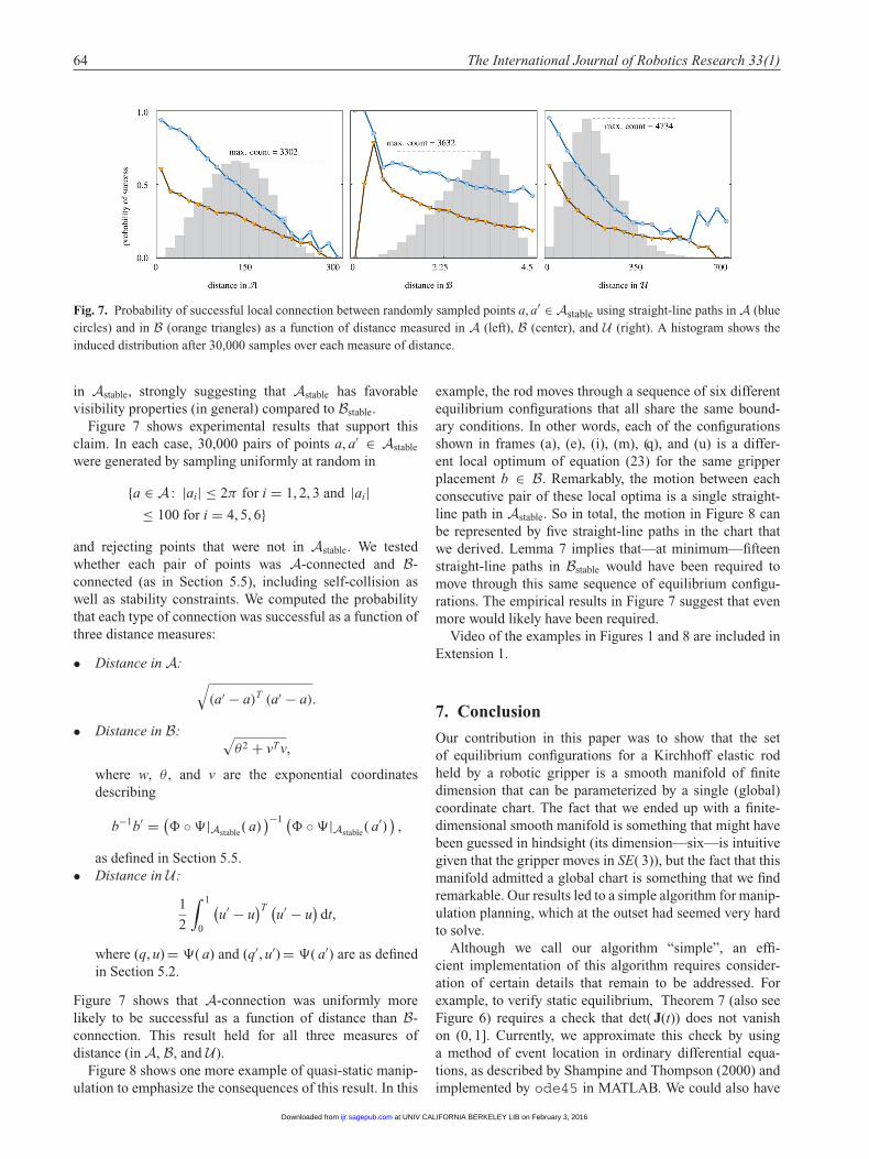
Fig. 7. Probability of successful local connection between randomly sampled points a, a′ ∈ Astable using straight-line paths in A (bluecircles) and in B (orange triangles) as a function of distance measured in A (left), B (center), and U (right). A histogram shows theinduced distribution after 30,000 samples over each measure of distance.

in Astable, strongly suggesting that Astable has favorablevisibility properties (in general) compared to Bstable.

Figure 7 shows experimental results that support thisclaim. In each case, 30,000 pairs of points a, a′ ∈ Astable

were generated by sampling uniformly at random in

{a ∈ A : |ai| ≤ 2π for i = 1, 2, 3 and |ai|≤ 100 for i = 4, 5, 6}

and rejecting points that were not in Astable. We testedwhether each pair of points was A-connected and B-connected (as in Section 5.5), including self-collision aswell as stability constraints. We computed the probabilitythat each type of connection was successful as a function ofthree distance measures:

• Distance in A: √(a′ − a)T (a′ − a).

• Distance in B: √θ2 + vT v,

where w, θ , and v are the exponential coordinatesdescribing

b−1b′ = (� ◦ �|Astable ( a)

)−1 (� ◦ �|Astable ( a′)

),

as defined in Section 5.5.• Distance in U:

1

2

∫ 1

0

(u′ − u

)T (u′ − u

)dt,

where (q, u) = �( a) and (q′, u′) = �( a′) are as definedin Section 5.2.

Figure 7 shows that A-connection was uniformly morelikely to be successful as a function of distance than B-connection. This result held for all three measures ofdistance (in A, B, and U).

Figure 8 shows one more example of quasi-static manip-ulation to emphasize the consequences of this result. In this

example, the rod moves through a sequence of six differentequilibrium configurations that all share the same bound-ary conditions. In other words, each of the configurationsshown in frames (a), (e), (i), (m), (q), and (u) is a differ-ent local optimum of equation (23) for the same gripperplacement b ∈ B. Remarkably, the motion between eachconsecutive pair of these local optima is a single straight-line path in Astable. So in total, the motion in Figure 8 canbe represented by five straight-line paths in the chart thatwe derived. Lemma 7 implies that—at minimum—fifteenstraight-line paths in Bstable would have been required tomove through this same sequence of equilibrium configu-rations. The empirical results in Figure 7 suggest that evenmore would likely have been required.

Video of the examples in Figures 1 and 8 are included inExtension 1.

7. Conclusion

Our contribution in this paper was to show that the setof equilibrium configurations for a Kirchhoff elastic rodheld by a robotic gripper is a smooth manifold of finitedimension that can be parameterized by a single (global)coordinate chart. The fact that we ended up with a finite-dimensional smooth manifold is something that might havebeen guessed in hindsight (its dimension—six—is intuitivegiven that the gripper moves in SE( 3)), but the fact that thismanifold admitted a global chart is something that we findremarkable. Our results led to a simple algorithm for manip-ulation planning, which at the outset had seemed very hardto solve.

Although we call our algorithm “simple”, an effi-cient implementation of this algorithm requires consider-ation of certain details that remain to be addressed. Forexample, to verify static equilibrium, Theorem 7 (also seeFigure 6) requires a check that det( J(t)) does not vanishon (0, 1]. Currently, we approximate this check by usinga method of event location in ordinary differential equa-tions, as described by Shampine and Thompson (2000) andimplemented by ode45 in MATLAB. We could also have




(a) (b) (c) (d) (e)

(e) (f) (g) (h) (i)

(i) (j) (k) (l) (m)

(m) (n) (o) (p) (q)

(q) (r) (s) (t) (u)

Fig. 8. Another example of quasi-static manipulation by robotic grippers (blue) of an elastic rod (orange), in which we are exploringa zoo of equilibrium configurations—shown in frames (a), (e), (i), (m), (q), and (u)—that all share the same boundary conditions.Remarkably, each row corresponds to a straight-line path in the global coordinate chart A that we derived.

approximated this check by sampling t at some fixed reso-lution. Neither approach is guaranteed to produce a correctresult, and both approaches suffer from the classic tradeoffbetween resolution (hence, computation time) and accuracy.We would much prefer to implement an adaptive or “exact”approach, as suggested—for example—by Schwarzer et al.(2005). Doing so is problematic, however, since det( J(t))and all its derivatives vanish at t = 0. Along similar lines,the computation of both J and q requires the integration oflinear, time-varying, matrix differential equations. Again,we have done so simply by using ode45 in MATLAB,with a sufficiently low error tolerance. Ignoring the obvi-ous structure in equations (25) and (33) makes our currentimplementation highly inefficient. The use of variational

integrators (West, 2004) would be a straightforward way toimprove performance.

There are several other opportunities for future work.First, the coordinates we derive can be interpreted as forcesand torques at the base of the elastic rod, so A is exactly thespace over which to perform inference in state estimationwith a force/torque sensor. Second, our model of an elas-tic rod depends on three physical parameters c1, c2, c3 > 0.Finding these parameters from observations of equilibriumconfigurations can be cast as an inverse optimal controlproblem (Javdani et al., 2011). The structure establishedby Theorem 6 allows us to define a notion of orthogo-nal distance between C and these observations, similar toKeshavarz et al. (2011), and may lead to an efficient method




of solution. Third, we note that an elastic inextensible strip(or “ribbon”) is a developable surface whose shape can bereconstructed from its centerline (Starostin and van der Hei-jden, 2008). This centerline conforms to a similar model asthe elastic rod and is likely amenable to similar analysis,which may generalize to models of other developable sur-faces. Finally, it may be possible to generalize our approachto deal with other applied forces. The consideration ofgravity—as the gradient of a potential—should be straight-forward, although it complicates our approach to Lie–Poisson reduction. The consideration of other forces arisingfrom interaction between different parts of the elastic rod(e.g. self-collision) is apparently much harder.

Notes

1. This model is slightly different from the one we describe inSection 5—for a discussion of the relationship between thesetwo models, see Biggs et al. (2007).

2. The smooth topology is also called the C∞ topology and theWhitney topology in the literature (Hirsch, 1976).

Funding

This work was supported by the National Science Foundation(grant numbers CPS-0931871 and CMMI-0956362).

Acknowledgements

The authors would like to thank Don Shimamoto for his manyhelpful comments, in particular those leading to the current proofof Lemma 4. Thanks also to the organizers, anonymous review-ers, and audience at WAFR 2012, whose suggestions helped toimprove this paper.

References

Agarwal P, Guibas L, Nguyen A, Russel D and Zhang L (2004)Collision detection for deforming necklaces. ComputationalGeometry 28(2–3): 137–163.

Agrachev AA and Sachkov YL (2004) Control Theory from theGeometric Viewpoint. Berlin: Springer.

Amato NM and Song G (2002) Using motion planning to studyprotein folding pathways. Journal of Computational Biology 9(2): 149–168.

Antman SS (2005) Nonlinear Problems of Elasticity. New York:Springer.

Asano Y, Wakamatsu H, Morinaga E, Arai E and Hirai S (2010)Deformation path planning for manipulation of flexible circuitboards. In: IEEE/RSJ international conference on intelligentrobots and systems (IROS ‘10), Taipei, Taiwan, 18–22 October2010, pp. 5386–5391. Piscataway: IEEE Press.

Balkcom DJ and Mason MT (2008) Robotic origami folding.International Journal of Robotics Research 27(5): 613–627.

Bell M and Balkcom D (2008) Knot tying with single piecefixtures. In: IEEE international conference on robotics andautomation (ICRA ‘08), Pasadena, CA, 19–23 May 2008, pp.379–384. Piscataway: IEEE Press.

Bergou M, Wardetzky M, Robinson S, Audoly B and Grinspun E(2008) Discrete elastic rods. ACM Transactions on Graphics 27(3): 1–12.

Biggs J, Holderbaum W and Jurdjevic V (2007) Singu-larities of optimal control problems on some 6-D Liegroups. IEEE Transactions on Automation and Control 52(6):1027–1038.

Bloch A, Krishnaprasad P, Marsden J and Ratiu T (1996) TheEuler–Poincaré equations and double bracket dissipation. Com-munications in Mathematical Physics 175(1): 1–42.

Bretl T and McCarthy Z (2012) Equilibrium configurations ofa Kirchhoff elastic rod under quasi-static manipulation. In:10th international workshop on the algorithmic foundations ofrobotics (WAFR ‘12), Cambridge, USA, 13–15 June 2012.

Camarillo DB, Milne CF, Carlson CR, Zinn MR and SalisburyJK (2008) Mechanics modeling of tendon-driven continuummanipulators. IEEE Transactions on Robotics 24(6): 1262–1273.

Chirikjian GS and Burdick JW (1995) The kinematics of hyper-redundant robot locomotion. IEEE Transactions on Roboticsand Automation 11(6): 781–793.

Choset H, Lynch K, Hutchinson S, Kanto G, Burgard W, KavrakiL et al. Principles of Robot Motion: Theory, Algorithms, andImplementations. Cambridge: MIT Press.

Clements TN and Rahn CD (2006) Three-dimensional contactimaging with an actuated whisker. IEEE Transactions onRobotics 22(4): 844–848.

Gopalakrishnan K and Goldberg K (2005) D-Space and deformclosure grasps of deformable parts. International Journal ofRobotics Research 24(11): 899–910.

Gottschalk S, Lin M and Manocha D (1996) OBB-tree: A hierar-chical structure for rapid interference detection. ComputationalGraphics 30: 171–180.

Henderson ME and Neukirch S (2004) Classification of the spatialequilibria of the clamped elastica: Numerical continuation ofthe solution set. International Journal of Bifurcation & Chaosin Applied Sciences & Engineering 14(4): 1223–1239.

Hirsch MW (1976) Differential Topology. Berlin: Springer-Verlag, pp. 34–35.

Hoffman KA (2004) Methods for determining stability in contin-uum elastic-rod models of DNA. Philosophical Transactions ofthe Royal Society of London. Series A: Mathematical, Physicaland Engineering Sciences 362(1820): 1301–1315.

Hopcroft JE, Kearney JK and Krafft DB (1991) A case study offlexible object manipulation. International Journal of RoboticsResearch 10(1): 41–50.

Inaba M. Hand eye coordination in rope handling. J. of RoboticsSociety Japan, 3(6): 32–41, 1985.

Ivey TA and Singer DA (1999) Knot types, homotopies andstability of closed elastic rods. Proceedings of the LondonMathematical Society 79(2): 429–450.

Jansen R, Hauser K, Chentanez N, van der Stappen F and Gold-berg K (2009) Surgical retraction of non-uniform deformablelayers of tissue: 2D robot grasping and path planning. In:IEEE/RSJ international conference on intelligent robots andsystems (IROS ‘09), St. Louis, MO., 10–15 October 2009, pp.4092–4097. Piscataway: IEEE Press.

Javdani S, Tandon S, Tang J, O’Brien JF and Abbeel P (2011)Modeling and perception of deformable one-dimensionalobjects. In: IEEE international conference on robotics andautomation (ICRA ‘11), Shanghai, China, 9–13 May 2011, pp.1607–1614. Piscataway: IEEE Press.

Jurdjevic V (2005) Integrable Hamiltonian Systems on ComplexLie Groups. Providence: American Mathematical Society.




Kavraki LE, Svetska P, Latombe J-C and Overmars M (1996)Probabilistic roadmaps for path planning in high-dimensionalconfiguration spaces. IEEE Transactions on Robotics andAutomation 12(4): 566–580.

Keshavarz A, Wang Y and Boyd S (2011) Imputing a convexobjective function. In: IEEE multi-conference on systems andcontrol, Denver, CO., 28–30 September 2011, pp. 613–619.Piscataway: IEEE Press.

Lamiraux F and Kavraki LE (2001) Planning paths for elasticobjects under manipulation constraints. International Journalof Robotics Research 20(3): 188–208.

Langer J and Singer D (1984) The total squared curvature ofclosed curves. Journal of Differential Geometry 20: 1–22.

Langer J and Singer DA (1996) Lagrangian aspects of the Kirch-hoff elastic rod. SIAM Review 38(4): 605–618.

Latombe JC (1991) Robot Motion Planning. Boston: KluwerAcademic Publishers.

LaValle SM (2006) Planning Algorithms. New York: CambridgeUniversity Press.

Lee JM (2003) Introduction to Smooth Manifolds. New York:Springer.

Lin Q, Burdick J and Rimon E (2000) A stiffness-based qualitymeasure for compliant grasps and fixtures. IEEE Transactionson Robotics and Automation 16(6): 675–688.

Marsden JE and Ratiu TS (1999) Introduction to Mechanicsand Symmetry: A Basic Exposition of Classical MechanicalSystems. New York: Springer.

McCarthy Z and Bretl T (2012) Mechanics and manipulation ofplanar elastic kinematic chains. In: IEEE international confer-ence on robotics and automation (ICRA ‘12), St. Paul, USA,14–18 May 2012, pp. 2798–2805. Piscataway: IEEE Press.

Moll M and Kavraki LE (2006) Path planning fordeformable linear objects. IEEE Transactions on Robotics 22(4): 625–636.

Murray R, Li ZX and Sastry S (1994) A Mathematical Introduc-tion to Robotic Manipulation. Boca Raton: CRC Press.

Neukirch S and Henderson M (2002) Classification of the spatialequilibria of the clamped elastica: Symmetries and zoology ofsolutions. Journal of Elasticity 68(1): 95–121.

Pontryagin LS, Boltyanskii VG, Gamkrelidze RV andMishchenko EF (1962) The Mathematical Theory of OptimalProcesses. New York: Wiley.

Rucker DC, Webster RJ, Chirikjian GS and Cowan NJ(2010) Equilibrium conformations of concentric-tube contin-uum robots. International Journal of Robotics Research 29(10): 1263–1280

Sachkov Y (2008a) Conjugate points in the Euler elasticproblem. Journal of Dynamical and Control Systems 14(3): 409–439.

Sachkov Y (2008b) Maxwell strata in the Euler elastic problem.Journal of Dynamical and Control Systems 14(2): 169–234.

Saha M and Isto P (2007) Manipulation planning for deformablelinear objects. IEEE Transactions on Robotics 23(6):1141–1150.

Sánchez G and Latombe J-C (2002) On delaying collision check-ing in PRM planning: Application to multi-robot coordination.International Journal of Robotics Research 21(1): 5–26.

Schwarzer F, Saha M and Latombe JC (2005) Adaptive dynamiccollision checking for single and multiple articulated robotsin complex environments. IEEE Transactions on Robotics 21(3): 338–353.

Shampine L and Thompson S (2000) Event location for ordi-nary differential equations. Computers & Mathematics withApplications 39(5–6): 43–54.

Shi Y and Hearst JE (1994) The Kirchhoff elastic rod, the non-linear Schrödinger equation, and DNA supercoiling. Journal ofChemical Physics 101(6): 5186–5200.

Shi Y, Hearst JE, Bishop TC and Halvorson HR (1998) Erratum:“the Kirchhoff elastic rod, the nonlinear Schrödinger equation,and DNA supercoiling” [J. Chem. Phys. 101, 5186 (1994)].Journal of Chemical Physics 109(7): 2959–2961.

Solomon JH and Hartmann MJZ (2010) Extracting objectcontours with the sweep of a robotic whisker using torqueinformation. International Journal of Robotics Research 29(9): 1233–1245.

Souéres P and Boissonnat J (1998) Optimal trajectories for non-holonomic mobile robots. In: Laumond J-P (ed) Robot MotionPlanning and Control. Berlin: Springer, vol. 229, ch. 3, pp.93–170.

Starostin EL and van der Heijden GHM (2008) Tension-inducedmultistability in inextensible helical ribbons. Physical ReviewLetters 101(8): 084301.

Takamatsu J, Morita T, Ogawara K, Kimura H and Ikeuchi K(2006) Representation for knot-tying tasks. IEEE Transactionson Robotics 22(1): 65–78.

Tanner H (2006) Mobile manipulation of flexible objects underdeformation constraints. IEEE Transactions on Robotics 22(1): 179–184.

van den Berg J, Miller S, Goldberg K and Abbeel P(2011) Gravity-based robotic cloth folding. AlgorithmicFoundations of Robotics IX Springer Tracts in AdvancedRobotics Volume 68, 2011, pp 409–424 Editors: Hsu,David; Isler, Volkan; Latombe, Jean-Claude; Lin, MingC. http://dx.doi.org/10.1007/978-3-642-17452-0_24 SpringerBerlin Heidelberg

Wakamatsu H, Arai E and Hirai S (2006) Knotting/unknottingmanipulation of deformable linear objects. International Jour-nal of Robotics Research 25(4): 371–395.

Walsh G, Montgomery R and Sastry S (1994) Optimal path plan-ning on matrix Lie groups. In: IEEE conference on decisionand control, Lake Buena Vista, FL., 14–16 December 1994,vol. 2, pp. 1258–1263. Piscataway: IEEE Press.

Webster RJ and Jones BA (2010) Design and kinematicmodeling of constant curvature continuum robots: Areview. International Journal of Robotics Research 29(13):1661–1683

West M (2004) Variational integrators. PhD Thesis, CaliforniaInstitute of Technology, USA.

Yamakawa Y, Namiki A and Ishikawa M (2011) Motion plan-ning for dynamic folding of a cloth with two high-speedrobot hands and two high-speed sliders. In: IEEE interna-tional conference on robotics and automation (ICRA ‘11),Shanghai, China, 9–13 May 2011, pp. 5486–5491. Piscataway:IEEE Press.




Appendix: Index to Multimedia Extensions

The multimedia extension page is found at www.ijrr.org

Table of Multimedia Extensions

Extension Media Type Description

1 Video Five examples of quasi-staticmanipulation. This video showsfive examples of quasistatic manip-ulation. The first three examplesshould clarify the differencebetween a “straight-line path” inthe space of boundary conditionsand in the global coordinate chartthat we derive in the paper. Thelast two examples correspond toFigures 1 and 8 in the paper.


http://www.ijrr.org/ijrr_2014/473169.htm


people.eecs.berkeley.eduzmccarthy/pdfs/bretl... · · 2016-02-03article quasi-static manipulation...

Documents