热传导问题基本算法 heat conduction algorithms

热传导问题 · 基本算法Heat Conduction · Algorithms

Dongke Sun (孙东科)[email protected]

东南大学机械工程学院School of Mechanical Engineering

Southeast University

January 31, 2019

Introduction

OUTLINE

1 Introduction

2 Steady One-dimensional ConductionBasic Equations, Grid Spacing and Interface ConductivityNonlinearity and Source Term LinearizationBoundary Conditions and Solutions of the LA Equations

3 Unsteady One-dimensional ConductionThe General Discretization EquationExplicit, Crank-Nicolson, and Fully Implicit Schemes

4 Two- and Three-dimensional SituationsDiscretization Equation for Two DimensionsDiscretization Equation for Three DimensionsSolution of the Linear Algebraic Equations

5 Over-Relaxation and Under-Relaxation

Dongke Sun (Southeast University) January 31, 2019 2 / 64

Introduction

Introduction

Heat conduction in the steady state

The governing equation can easily be derived𝜕𝑇

𝜕𝑡= ∇ · (𝑘∇𝑇 ) + 𝑆𝑇


Steady One-dimensional Conduction

OUTLINE

1 Introduction






Steady One-dimensional Conduction Basic Equations, Grid Spacing and Interface Conductivity

OUTLINE

1 Introduction







The Basic Equations

Application of the method is 1-D steady state heat transfer problems

d

d𝑥

(︂𝑘

d𝑇

d𝑥

)︂+ 𝑆 = 0 (1)

This leads to the discretization equation

𝑎𝑃𝑇𝑃 = 𝑎𝐸𝑇𝐸 + 𝑎𝑊𝑇𝑊 + 𝑏 (2)

where

𝑎𝐸 =𝑘𝑒

(𝛿𝑥)𝑒, 𝑎𝑊 =

𝑘𝑒(𝛿𝑥)𝑤

, 𝑎𝑃 = 𝑎𝐸 + 𝑎𝑊 − 𝑆𝑃∆𝑥, 𝑏 = 𝑆𝐶∆𝑥 (3)

The quantities 𝑆𝐶 and 𝑆𝑃 arise from the source-term linearization of theform

𝑆 = 𝑆𝐶 + 𝑆𝑃𝑇𝑃 (4)

The value 𝑇𝑃 is assumed to be prevail throughout the control volume.



The Grid Spacing

Grid-point cluster for the 1-D problemIt is now necessary that he distances (𝛿𝑥)𝑒 and (𝛿𝑥)𝑤 be equal.A fine grid is required where the 𝑇 ∼ 𝑥 variation is steep.

Since the 𝑇 ∼ 𝑥 distribution is unknown before the problem is solved, howcan we design an appropriate nun-uniform grid?

1 We normally has some qualitative expectations about the solution,from which some guidance can be obtained.

2 Preliminary coarse-grid solutions can be used to find pattern of the𝑇 ∼ 𝑥 variation; a suitable non-uniform grid can be used toconstructed.



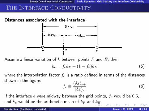
The Interface Conductivity

Distances associated with the interface

Assume a linear variation of 𝑘 between points 𝑃 and 𝐸, then

𝑘𝑒 = 𝑓𝑒𝑘𝑃 + (1 − 𝑓𝑒)𝑘𝐸 (5)

where the interpolation factor 𝑓𝑒 is a ratio defined in terms of the distancesshown in the figure:

𝑓𝑒 ≡(𝛿𝑥)𝑒+(𝛿𝑥)𝑒

(6)

If the interface 𝑒 were midway between the grid points, 𝑓𝑒 would be 0.5,and 𝑘𝑒 would be the arithmetic mean of 𝑘𝑃 and 𝑘𝐸 .




A problem: This simple-minded approach leads to rather incorrectimplications in some cases and cannot accurately handle the abruptchanges of conductivity that may occur in composite materials.

Our main objective is to obtain a good representation for the heat flux𝑞𝑒 at the interface via

𝑞𝑒 =𝑘𝑒(𝑇𝑃 − 𝑇𝐸)

(𝛿𝑥)𝑒(7)

A steady 1-D anaylysis (without sources) leads to

𝑞𝑒 =𝑇𝑃 − 𝑇𝐸

(𝛿𝑥)𝑒−/𝑘𝑃 + (𝛿𝑥)𝑒+/𝑘𝐸(8)

Combination of above Eqs yields

𝑞𝑒 =

(︂1 − 𝑓𝑒𝑘𝑃

+𝑓𝑒𝑘𝐸

)︂−1

. (9)

When the interface 𝑒 is placed midway between 𝑃 and 𝐸, 𝑓𝑒 = 0.5.




Then𝑘−1𝑒 = 0.5(𝑘−1

𝑃 + 𝑘−1𝐸 ) or 𝑘𝑒 =

2𝑘𝑃𝑘𝐸𝑘𝑃 + 𝑘𝐸

. (10)

It shows that the 𝑘𝑒 is the harmonic mean of 𝑘𝑃 and 𝑘𝐸 , rather than thearithmetic mean.The use of Eq.(9) leads to the following expression for 𝑎𝐸

𝑎𝐸 =

[︂(𝛿𝑥)𝑒−𝑘𝑃

+(𝛿𝑥)𝑒+𝑘𝐸

]︂(11)

Clearly, 𝑎𝐸 represent the conductace of the materials between points 𝑃 and𝐸. A similar expression can be written for 𝑎𝑊

𝑎𝑊 =

[︂(𝛿𝑥)𝑤−𝑘𝑊

+(𝛿𝑥)𝑤+

𝑘𝑃

]︂The effectiveness of this formulation can be quickly seen in the twofollowing limiting cases.




1 Let 𝑘𝐸 → 0. Then, from Eq. (9)

𝑘𝑒 → 0 (12)

It implies that the heat flux at the face of an insulator becomes zero.The arithmetic mean formulation have given a nonzero flux in thissituation.

2 Let 𝑘𝑃 ≫ 𝑘𝐸 . Then

𝑘𝑒 →𝑘𝐸𝑓𝑒

(13)

It implies that 𝑘𝑒 is not equal to 𝑘𝐸 , but rather 1/𝑓𝑒 times it. Ourpurpose is to get a correct value of 𝑞𝑒 via Eq. (7). The use of Eq.(13) yields

𝑞𝑒 =𝑘𝐸(𝑇𝑃 − 𝑇𝐸)

(𝛿𝑥)𝑒+. (14)

When 𝑘𝑃 ≪ 𝑘𝐸 , the 𝑇𝑃 will prevail right up to the interface 𝑒.


Steady One-dimensional Conduction Nonlinearity and Source Term Linearization

OUTLINE

1 Introduction







Nonlinearity

The discretization equation 𝑎𝑃𝑇𝑃 = 𝑎𝐸𝑇𝐸 + 𝑎𝑊𝑇𝑊 + 𝑏 is a linearalgebraic equation, and we shall solve the set of such equations for linearequations. However, we shall frequently encounter nonlinear situationseven in heat conduction. The conductivity 𝑘 may depend on 𝑇 , or thesource 𝑆 may be a nonlinear function of 𝑇 .We shall handle such situations by iteration.

1 Start with a guess or estimate for the values of 𝑇 at all grid points.2 From these guessed 𝑇 s, calculate tentative values of the coefficients in

the discretization equation.3 Solve the nominally linear set of algebraic equations to get new values

of 𝑇 .4 With these 𝑇 s as better guesses, return step 2 and repeat the process

until further repetitions (called iterations) cease to produce anysignificant changes in the values of 𝑇 .

The final unchanging state if called the convergence of the iterations.



Source Term Linearization

The four possible linearizations for the example.


Steady One-dimensional Conduction Boundary Conditions and Solutions of the LA Equations

OUTLINE

1 Introduction







Boundary Conditions

Control volumes for the internal and boundary points.

Typically, three kinds of boundary conditions are encountered:Given boundary temperatureGiven boundary heat fluxBoundary heat flux specified via a heat transfer coefficient and thetemperature of surrounding fluid

Intergrating Eq (1) over the CV and noting that 𝑞 stands for −𝑘d𝑇/d𝑥, weget

𝑞𝐵 − 𝑞𝑖 + (𝑆𝐶 + 𝑆𝑃𝑇𝐵)∆𝑥 = 0 (15)

The interface heat flux 𝑞𝑖 can be written as 𝑞𝑖 = 𝑘𝑒(𝑇𝐵 − 𝑇𝐼)/(𝛿𝑥)𝑖. So,

𝑞𝐵 − 𝑘𝑖(𝑇𝐵 − 𝑇𝐼)

(𝛿𝑥)𝑖+ (𝑆𝐶 + 𝑆𝑃𝑇𝐵)∆𝑥 = 0 (16)



Boundary Conditions

If the value of 𝑞𝐵 itself is given, the required equation for 𝑇𝐵 becomes

𝑎𝐵𝑇𝐵 = 𝑎𝐼𝑇𝐼 + 𝑏 (17)

where𝑎𝐼 =

𝑘𝑖(𝛿𝑥)𝑖

, 𝑏 = 𝑆𝐶∆𝑥 + 𝑞𝐵, 𝑎𝐵 = 𝑎𝐼 − 𝑆𝑃∆𝑥 (18)

If the value of 𝑞𝐵 is specified in terms of a heat transfer coefficient ℎ and asurrounding-fluid temperature 𝑇𝑓 such that

𝑞𝐵 = ℎ(𝑇𝑓 − 𝑇𝐵) (19)

then the equation for 𝑇𝐵 becomes

𝑎𝐵𝑇𝐵 = 𝑎(𝑇𝐼 + 𝑏) (20)

where

𝑎𝐼 =𝑘𝑖

(𝛿𝑥)𝑖, 𝑏 = 𝑆𝐶∆𝑥 + ℎ𝑇𝑓 , 𝑎𝐵 = 𝑎𝐼 − 𝑆𝑃∆𝑥 + ℎ (21)



Solutions of the Linear Algebraic Equations

The TDMA (TriDiagonal-Matrix Algorithm)The discretization equations can be written as

𝑎𝑖𝑇𝑖 = 𝑏𝑖𝑇𝑖+1 + 𝑐𝑖𝑇𝑖−1 + 𝑑𝑖 (22)

To account for the special form of the boundary-point equations, let us set

𝑐1 = 0 and 𝑏𝑁 = 0 (23)

Suppose, in the forward-substitution process, we seek a relation

𝑇𝑖 = 𝑃𝑖𝑇𝑖+1 + 𝑄𝑖 (24)

after we have just obtained

𝑇𝑖−1 = 𝑃𝑖−1𝑇𝑖 + 𝑄𝑖−1 (25)

Substitution of Eq. (25) into Eq. (22) leads to

𝑎𝑖𝑇𝑖 = 𝑏𝑖𝑇𝑖+1 + 𝑐𝑖(𝑃𝑖−1𝑇𝑖 + 𝑄𝑖−1) + 𝑑𝑖 (26)



Solutions of the Linear Algebraic Equations

The coefficients 𝑃𝑖 and 𝑄𝑖 stand for

𝑃𝑖 =𝑏𝑖

𝑎𝑖 − 𝑐𝑖𝑃𝑖−1𝑄𝑖 =

𝑑𝑖 + 𝑐𝑖𝑄𝑖−1

𝑎𝑖 − 𝑐𝑖𝑃𝑖−1(27)

To start the recurrence process, we note that Eq. (22) for 𝑖 = 1 is almostof the form (24). Thus, the values of 𝑃1 and 𝑄1 are given by

𝑃1 =𝑏1𝑎1

and 𝑄1 =𝑑1𝑎1

(28)

It is interesting to note that these expressions do follow Eq. (27) after thesubstitution 𝑐𝑖 = 0.At the other end of the 𝑃𝑖, 𝑄𝑖 sequence, we note that 𝑏𝑁 = 0. This leadsto 𝑃𝑁 = 0, and hence from Eq. (24) we obtain

𝑇𝑁 = 𝑄𝑁 (29)

Now we are in a position to start the back substitution via Eq. (24).



Solutions of the Linear Algebraic EquationsSummary of the algorithm

1 Calculate 𝑃1 and 𝑄1 from Eq. (28).2 Use the recurrence relations (27), i.e.

𝑃𝑖 =𝑏𝑖

𝑎𝑖 − 𝑐𝑖𝑃𝑖−1𝑄𝑖 =

𝑑𝑖 + 𝑐𝑖𝑄𝑖−1

𝑎𝑖 − 𝑐𝑖𝑃𝑖−1

to obtain 𝑃𝑖 and 𝑄𝑖 for 𝑖 = 1, 2, 3, ..., 𝑁 .3 Set 𝑇𝑁 = 𝑄𝑁 .4 Use Eq. (24), i.e. 𝑇𝑖−1 = 𝑃𝑖−1𝑇𝑖 + 𝑄𝑖−1, for

𝑖 = 𝑁 − 1, 𝑁 − 2, 𝑁 − 3, ..., 3, 2, 1 to obtain𝑇𝑁−1, 𝑇𝑁−2, ..., 𝑇3, 𝑇2, 𝑇1.

The algorithm is a very powerful and convenient equation solverwhenever the algebraic equations can be represented in the form of Eq.(22).

Unlike general matrix methods, the TDMA requires computer storageand computer time proportional only to 𝑁 , rather than to 𝑁2 or 𝑁3.


Unsteady One-dimensional Conduction

OUTLINE

1 Introduction






Unsteady One-dimensional Conduction The General Discretization Equation

OUTLINE

1 Introduction







The General Discretization Equation

The unsteady one-dimensional heat-conduction equation

𝜌𝑐𝜕𝑇

𝜕𝑡=

𝜕

𝜕𝑥

(︂𝑘𝜕𝑇

𝜕𝑥

)︂(30)

The discretization equation is now derived by integrating Eq. (30) over thecontrol volume and over the time interval from 𝑡 to 𝑡 + ∆𝑡. Thus,

𝜌𝑐

ˆ 𝑒

𝑤

ˆ 𝑡+Δ𝑡

𝑡

𝜕𝑇

𝜕𝑡d𝑡d𝑥 =

ˆ 𝑡+Δ𝑡

𝑡

ˆ 𝑒

𝑤

𝜕

𝜕𝑥

(︂𝜕𝑇

𝜕𝑥

)︂d𝑥d𝑡 (31)

For the representation of the term 𝜕𝑇/𝜕𝑡, we shall assume that thegrid-point value of 𝑇 prevails throughout the control volume. Then

𝜌𝑐

ˆ 𝑒

𝑤

ˆ 𝑡+Δ𝑡

𝑡

𝜕𝑇

𝜕𝑡d𝑡d𝑥 = 𝜌𝑐∆𝑥(𝑇 1

𝑃 − 𝑇 0𝑃 ) (32)




Following our steady-state practice for 𝑘𝜕𝑇/𝜕𝑥, we obtain

𝜌𝑐∆𝑥(𝑇 1𝑃 − 𝑇 0

𝑃 ) =

ˆ 𝑡+Δ𝑡

𝑡

[︂𝑘𝑒(𝑇𝐸 − 𝑇𝑃 )

(𝛿𝑥)𝑒− 𝑘𝑤(𝑇𝑃 − 𝑇𝑊 )

(𝛿𝑥)𝑤

]︂d𝑡 (33)

It is at this point that we need assumptions about how 𝑇𝑃 , 𝑇𝐸 and 𝑇𝑊

vary with time from 𝑡 to 𝑡 + ∆𝑡. Some of assumptions can be generalizedby proposing ˆ 𝑡+Δ𝑡

𝑡𝑇𝑝d𝑡 = [𝑓𝑇 1

𝑝 + (1 − 𝑓)𝑇 0𝑃 ]∆𝑡 (34)

where 𝑓 is a weighting factor between 0 and 1.

𝜌𝑐∆𝑥

∆𝑡(𝑇 1

𝑃 − 𝑇 0𝑃 ) = 𝑓

[︂𝑘𝑒(𝑇

1𝐸 − 𝑇 1

𝑃 )

(𝛿𝑥)𝑒−

𝑘𝑤(𝑇 1𝑃 − 𝑇 1

𝑊 )

(𝛿𝑥)𝑤

]︂+

(1 − 𝑓)

[︂𝑘𝑒(𝑇

0𝐸 − 𝑇 0

𝑃 )

(𝛿𝑥)𝑒−

𝑘𝑤(𝑇 0𝑃 − 𝑇 0

𝑊 )

(𝛿𝑥)𝑤

]︂ (35)


Unsteady One-dimensional Conduction Explicit, Crank-Nicolson, and Fully Implicit Schemes

OUTLINE

1 Introduction








After rearrangement the above equation, we have

𝑎𝑃𝑇𝑃 = 𝑎𝐸 [𝑓𝑇𝐸 + (1 − 𝑓)𝑇 0𝐸 ] + 𝑎𝑊 [𝑓𝑇𝑊 + (1 − 𝑓)𝑇 0

𝑊 ]

+ [𝑎0𝑃 − (1 − 𝑓)𝑎𝐸 − (1 − 𝑓)𝑎𝑊 ]𝑇 0𝑃

(36)

where𝑎𝐸 =

𝑘𝑒(𝛿𝑥)𝑒

, 𝑎𝑊 =𝑘𝑤

(𝛿𝑥)𝑤, 𝑎0𝑃 =

𝜌𝑐∆𝑥

∆𝑡

𝑎𝑃 = 𝑓𝑎𝐸 + 𝑓𝑎𝑊 + 𝑎0𝑃

(37)

For certain specific values of the weighting factor 𝑓 , the discretizationequation reduces to one of the well-known schemes for parabolic equations.In particular.

𝑓 = 0 leads to the explicit scheme,𝑓 = 1/2 to the Crank-Nicolson scheme,𝑓 = 1 to the fully implicit scheme.



Three Different Schemes

Variation of temperature with time for three different schemes



Three Different Schemes

Variation of temperature with time for three different schemes

The explicit scheme assumes that the old value 𝑇 0𝑃 prevails throughout

the entire time step except at time 𝑡 + ∆𝑡.The Crank-Nicolson scheme assumes a linear variation of 𝑇𝑃 .The fully implicit scheme postulates that 𝑇𝑃 suddenly drops from 𝑇 0

𝑃

to 𝑇 1𝑃 at time 𝑡, and then stays at 𝑇 1

𝑃 over the whole of the time step.



Explicit Scheme and Full Implicit Scheme

For the Explicit Scheme, Eq. (36) becomes

𝑎𝑃𝑇𝑃 = 𝑎𝐸𝑇0𝐸 + 𝑎𝑊𝑇 0

𝑊 + (𝑎0𝑃 − 𝑎𝐸 − 𝑎𝑊 )𝑇 0𝑃 (38)

For uniform conductivity and ∆𝑥 = (𝛿𝑥)𝑒 = (𝛿𝑥)𝑤, the condition can beexpressed as

∆𝑡 <𝜌𝑐(∆𝑥)2

2𝑘(39)

Here we record the Full Implicit Scheme of Eq. (36). We shall introducethe linearized source term, which we had temporarily dropped. The result is

𝑎𝑃𝑇𝑃 = 𝑎𝐸𝑇𝐸 + 𝑎𝑊𝑇𝑊 + 𝑏 (40)

with

𝑎𝐸 =𝑘𝑒

(𝛿𝑥)𝑒, 𝑎𝑊 =

𝑘𝑤(𝛿𝑥)𝑤

, 𝑎0𝑃 =𝜌𝑐∆𝑥

∆𝑡, 𝑏 = 𝑆𝐶∆𝑥 + 𝑎0𝑃𝑇

0𝑃

𝑎𝑃 = 𝑎𝐸 + 𝑎𝑊 + 𝑎0𝑃 − 𝑆𝑃∆𝑥

(41)


Two- and Three-dimensional Situations

OUTLINE

1 Introduction






Two- and Three-dimensional Situations Discretization Equation for Two Dimensions

OUTLINE

1 Introduction







Discretization Equation for Two Dimensions

The differential equation for two-dimensional situation is

𝜌𝑐𝜕𝑇

𝜕𝑡=

𝜕

𝜕𝑥

(︂𝑘𝜕𝑇

𝜕𝑥

)︂+

𝜕

𝜕𝑦

(︂𝑘𝜕𝑇

𝜕𝑦

)︂+ 𝑆 (42)



Discretization Equation for Two Dimensions

The differential equation for two-dimensional situation is

𝜌𝑐𝜕𝑇

𝜕𝑡=

𝜕

𝜕𝑥

(︂𝑘𝜕𝑇

𝜕𝑥

)︂+

𝜕

𝜕𝑦

(︂𝑘𝜕𝑇

𝜕𝑦

)︂+ 𝑆 (42)

The discretization equation

𝑎𝑃𝑇𝑃 = 𝑎𝐸𝑇𝐸 + 𝑎𝑊𝑇𝑊 + 𝑎𝑁𝑇𝑁 + 𝑎𝑆𝑇𝑆 + 𝑏 (43)

where𝑎𝐸 =

𝑘𝑒∆𝑦

(𝛿𝑥)𝑒𝑎𝑁 =

𝑘𝑛∆𝑥

(𝛿𝑥)𝑛

𝑎𝑊 =𝑘𝑤∆𝑦

(𝛿𝑥)𝑤𝑎𝑆 =

𝑘𝑠∆𝑥

(𝛿𝑥)𝑠

𝑎0𝑃 =𝜌𝑐∆𝑥∆𝑦

∆𝑡𝑏 = 𝑆𝐶∆𝑥∆𝑦 + 𝑎0𝑃𝑇

0𝑃

𝑎𝑃 = 𝑎𝐸 + 𝑎𝑊 + 𝑎𝑁 + 𝑎𝑆 + 𝑎0𝑃 − 𝑆𝑃∆𝑥∆𝑦

(44)

The product ∆𝑥∆𝑦 is the volume of the control volume.


Two- and Three-dimensional Situations Discretization Equation for Three Dimensions

OUTLINE

1 Introduction






Two- and Three-dimensional Situations Discretization Equation for Three Dimensions

Discretization Equation for Three Dimensions

The differential equation for three-dimensional situation is

𝜌𝑐𝜕𝑇

𝜕𝑡=

𝜕

𝜕𝑥

(︂𝑘𝜕𝑇

𝜕𝑥

)︂+

𝜕

𝜕𝑦

(︂𝑘𝜕𝑇

𝜕𝑦

)︂+

𝜕

𝜕𝑧

(︂𝑘𝜕𝑇

𝜕𝑧

)︂+ 𝑆

The discretization equation

𝑎𝑃𝑇𝑃 = 𝑎𝐸𝑇𝐸 + 𝑎𝑊𝑇𝑊 + 𝑎𝑁𝑇𝑁 + 𝑎𝑆𝑇𝑆 + 𝑎𝑇𝑇𝑇 + 𝑎𝐵𝑇𝐵 + 𝑏 (45)

where

𝑎𝐸 =𝑘𝑒∆𝑦∆𝑧

(𝛿𝑥)𝑒𝑎𝑁 =

𝑘𝑛∆𝑧∆𝑥

(𝛿𝑥)𝑛𝑎𝑇 =

𝑘𝑡∆𝑥∆𝑦

(𝛿𝑥)𝑡

𝑎𝑊 =𝑘𝑤∆𝑦∆𝑧

(𝛿𝑥)𝑤𝑎𝑆 =

𝑘𝑠∆𝑧∆𝑥

(𝛿𝑥)𝑠𝑎𝐵 =

𝑘𝑏∆𝑥∆𝑦

(𝛿𝑥)𝑏

𝑎0𝑃 =𝜌𝑐∆𝑥∆𝑦∆𝑧

∆𝑡𝑏 = 𝑆𝐶∆𝑥∆𝑦∆𝑧 + 𝑎0𝑃𝑇

0𝑃

𝑎𝑃 = 𝑎𝐸 + 𝑎𝑊 + 𝑎𝑁 + 𝑎𝑆 + 𝑎𝑇 + 𝑎𝐵 + 𝑎0𝑃 − 𝑆𝑃∆𝑥∆𝑦∆𝑧

(46)


Two- and Three-dimensional Situations Solution of the Linear Algebraic Equations

OUTLINE

1 Introduction







The Gauss-Seidel Point-by-Point Method

The simplest of all iterative methods is the Gauss-Seidel method in whichthe values of the variable are calculated by visiting each grid point in acertain order. The discretization equation is written as

𝑎𝑃𝑇𝑃 =∑︁

𝑎nb𝑇nb + 𝑏 (47)

where the subscript nb denotes a neighbor point, the 𝑇𝑃 at the visited gridpoint is calculated from

𝑇𝑃 =

∑︀𝑎nb𝑇

*nb + 𝑏

𝑎𝑃(48)

where 𝑇 *nb stands for the neighbor-point value present in the computer

storage. In any case, 𝑇 *nb is the latest available value for the neighbor-point

temperature.When all grid points have been visited in this manner, one iteration of theGauss-Seidel method is complete.Dongke Sun (Southeast University) January 31, 2019 36 / 64



To illustrate the method, we shall consider two very simple exampleCase 1:Equations 𝑇1 = 0.4𝑇2 + 0.2, 𝑇2 = 𝑇1 + 1 (49)

Solution————————————————————————————–

————————————————————————————–

Case 2:Equations 𝑇1 = 𝑇2 − 1, 𝑇2 = 2.5𝑇1 − 0.5 (50)

Solution————————————————————————————–

————————————————————————————–




To illustrate the method, we shall consider two very simple exampleCase 1:Equations 𝑇1 = 0.4𝑇2 + 0.2, 𝑇2 = 𝑇1 + 1 (49)

Solution————————————————————————————–

————————————————————————————–

Case 2:Equations 𝑇1 = 𝑇2 − 1, 𝑇2 = 2.5𝑇1 − 0.5 (50)

Solution————————————————————————————–

————————————————————————————–Dongke Sun (Southeast University) January 31, 2019 37 / 64



The Causs-Seidel method does not always converge. The Scarboroughcriterion has been formulated∑︀

|𝑎nb||𝑎𝑃 |

=

{︂6 1 for all equations< 1 for at least one equation. (51)

Comments1 The criterion is a sufficient condition, not a necessary one.2 Although we shall not advocate the use of Gauss-Seidel method, it

seems desirable that our discretization equations should satisfy theScarborough criterion.

3 The presentce of a negative 𝑆𝑃 leads to∑︀

𝑎nb/𝑎𝑃 < 1 (𝑎𝑃 oftenequals

∑︀𝑎nb,

∑︀𝑎nb <

∑︀|𝑎nb|), which leads to a violation of the

criterion.4 when 𝑎𝑃 =

∑︀𝑎nb and all the coefficients are positive, we obtain∑︀

|𝑎nb|/|𝑎𝑃 | = 1 for all equations. The equation on boundaryconditions should satisfy

∑︀|𝑎nb|/|𝑎𝑃 | < 1.


Over-Relaxation and Under-Relaxation

OUTLINE

1 Introduction








Use of a relaxation factorWe shall introduce over-relaxation or under-relaxation with the generaldiscretization equation of the form

𝑎𝑃𝑇𝑃 =∑︁

𝑎nb𝑇nb + 𝑏 (52)

Further, 𝑇 *𝑃 will be taken as the value of 𝑇𝑃 from the previous iterations.

Eq. (52) can be written as

𝑇𝑃 =

∑︀𝑎nb𝑇nb + 𝑏

𝑎𝑃(53)

If we add 𝑇 *𝑃 to the right-hand side and subtract it, we have

𝑇𝑃 = 𝑇 *𝑃 +

(︂∑︀𝑎nb𝑇nb + 𝑏

𝑎𝑃− 𝑇 *

𝑃

)︂(54)

where the contents of the parentheses represent the change in 𝑇𝑃 producedby the current iteration.Dongke Sun (Southeast University) January 31, 2019 40 / 64



This change can be modified by the introduction of a relaxation factor 𝛼,so that

𝑇𝑃 = 𝑇 *𝑃 + 𝛼

(︂∑︀𝑎nb𝑇nb + 𝑏

𝑎𝑃− 𝑇 *

𝑃

)︂or

𝑎𝑃𝛼

𝑇𝑃 =∑︁

𝑎nb𝑇nb + 𝑏 + (1 − 𝛼)𝑎𝑃𝛼

𝑇 *𝑃

(55)

When the iterations converge, 𝑇𝑃 becomes equal to 𝑇 *𝑃 . The above

equation implies that the converged values do satisfy the originalequation.When the relaxation factor 𝛼 is between 0 and 1, its effect is under-relaxation. That is, the values of 𝑇𝑃 stay closer to 𝑇 *

𝑃 . When 𝛼 isgreater than 1, over-relaxation is produced.There is no need to maintain the same value of 𝛼 during the entirecomputation.It is permissible, though not very convenient, to choose a differentvalue of 𝛼 for each gird point.




Relaxation through inertiaAnother technique of over-Relaxation or under-Relaxation is to replace thediscretization equation (52) with

(𝑎𝑃 + 𝑖)𝑇𝑃 =∑︁

𝑎nb𝑇nb + 𝑏 + 𝑖𝑇 *𝑃 (56)

where 𝑖 is the so-called inertia.For positive values of 𝑖, Eq. (56) has the effect of under-relaxation,

while negative values of 𝑖 produce over-relaxation.There is no general rules for finding the optimum value of the inertia 𝑖.From Eq. (56), we can deduce that 𝑖 should be comparable to 𝑎𝑃 ,and the greater the magnitude of 𝑖 the stronger will be the effect ofthe relaxation.

The practice of solving a steady-state problem via the unsteadyformulation can now be recognized as simply a particular kind ofunder-relaxation procedure.


热传导问题 · 潜热处理Heat Conduction · Latent Heat

Dongke Sun (孙东科)[email protected]

东南大学机械工程学院School of Mechanical Engineering

Southeast University

January 31, 2019

Introduction

OUTLINE

6 Introduction

7 Governing Equation

8 In the Polar Coordinates

9 Worked Examples

10 Summary


Introduction

Introduction

Heat Transfer with Phase ChangeMelting/freezing/boiling/condensing takes place over an extended range oftemperatures.

The solid and liquid phases are separate by a two-phase moving region,"mushy zone".


Introduction

Introduction

Solidification of Metals and AlloysWe will describe the methods for solving alloy solidification problems inmultidimensional coordinate systems.

For the sake of simplicity, we will consider solidification problems withoutfluid flows.Dongke Sun (Southeast University) January 31, 2019 46 / 64

Governing Equation

OUTLINE

6 Introduction



9 Worked Examples

10 Summary


Governing Equation

Governing equation with a source term

Governing equation involving latent heatThe governing heat conduction equation can be cast into the weak form

𝜕(𝜌𝐻)

𝜕𝑡= ∇ · (𝑘∇𝑇 ) . (57)

The total enthalpy 𝐻 and the temperature 𝑇 can be interpreted asaveraged values within a control volume. Then,

𝐻 = 𝑐𝑝𝑇 + 𝑓𝑙𝐿ℎ (58)

where 𝑓𝑙 is the liquid phase fraction. For a system with liquid and solidphases, we have 𝑓𝑙 + 𝑓𝑠 = 1. Supposing 𝑐𝑝, 𝜌 = const, we obtain

𝜌𝑐𝑝𝜕𝑇

𝜕𝑡= ∇ · (𝜆∇𝑇 ) + 𝜌𝐿ℎ

𝜕𝑓𝑠𝜕𝑡

. (59)

The are three methods for solving the source term.


Governing Equation

Methods for solving source term

1 Equivalent Specific Heat Method


𝜕𝑡= ∇ · (𝜆∇𝑇 ) + 𝜌𝐿ℎ


(3)

Let make a variation𝜌𝐿ℎ


= 𝜌𝐿ℎ𝜕𝑓𝑠𝜕𝑇

𝜕𝑇

𝜕𝑡(4)

After substitution, we have

𝜌

(︂𝑐𝑝 − 𝐿ℎ

𝜕𝑓𝑠𝜕𝑇

)︂𝜕𝑇

𝜕𝑡= ∇ · (𝜆∇𝑇 ) (5)

Rearrange it. Then

𝜌𝑐𝑝𝑒𝜕𝑇

𝜕𝑡= ∇ · (𝜆∇𝑇 ) with 𝑐𝑝𝑒 = 𝑐𝑝 − 𝐿ℎ


(6)

How can we get the relation between solid fraction and 𝑇 , 𝑓𝑠 ∼ 𝑇?


Governing Equation

Heat Transfer with Phase Change

2 Temperature Recovery Method

𝜌𝑐𝑝𝜕𝑇 ′

𝜕𝑡= ∇ · (𝜆∇𝑇 ) ⇒

𝑇2 =𝑐𝑝𝑇

′2 + 𝐿ℎ

𝜕𝑓𝑠𝜕𝑇 (𝑇1 − 𝑇 ′

2)

𝑐𝑝 − 𝐿ℎ𝜕𝑓𝑠𝜕𝑇

for (a)

𝑇2 =𝑐𝑝𝑇

′2 + 𝐿ℎ

𝜕𝑓𝑠𝜕𝑇 (𝑇𝑙 − 𝑇 ′

2)


for (b)


Governing Equation



𝜌𝑐𝑝𝜕𝑇 ′

𝜕𝑡= ∇ · (𝜆∇𝑇 ) ⇒

𝑇2 =𝑐𝑝𝑇

′2 + 𝐿ℎ

𝜕𝑓𝑠𝜕𝑇 (𝑇𝑙 − 𝑇𝑠)


for (c)

𝑇2 =𝑐𝑝𝑇

′2 + 𝐿ℎ

𝜕𝑓𝑠𝜕𝑇 (𝑇1 − 𝑇𝑠)


for (d)


Governing Equation



𝑇2 =𝑐𝑝𝑇

′2 + 𝐿ℎ

𝜕𝑓𝑠𝜕𝑇 (𝑇1 − 𝑇 ′

2)


for (a) 𝑇2 =𝑐𝑝𝑇

′2 + 𝐿ℎ

𝜕𝑓𝑠𝜕𝑇 (𝑇𝑙 − 𝑇 ′

2)


for (b)

𝑇2 =𝑐𝑝𝑇

′2 + 𝐿ℎ

𝜕𝑓𝑠𝜕𝑇 (𝑇𝑙 − 𝑇𝑠)


for (c) 𝑇2 =𝑐𝑝𝑇

′2 + 𝐿ℎ

𝜕𝑓𝑠𝜕𝑇 (𝑇1 − 𝑇𝑠)

𝑐𝑝for (d)


Governing Equation


3 Enthalpy Method

Substitute𝜕𝐻

𝜕𝑇= 𝑐𝑝 − 𝐿ℎ


into 𝜌

(︂𝑐𝑝 − 𝐿ℎ


)︂𝜕𝑇

𝜕𝑡= ∇ · (𝜆∇𝑇 )

we obtain 𝜌𝜕𝐻

𝜕𝑇

𝜕𝑇

𝜕𝑡= ∇ · (𝜆∇𝑇 ) ⇒ 𝜌

𝜕𝐻

𝜕𝑡= ∇ · (𝜆∇𝑇 ) (7)

Then,𝐻𝑡+Δ𝑡

𝑖 −𝐻𝑡𝑖

∆𝑡=

𝜆

𝜌

𝑇 𝑡𝑖−1 − 2𝑇 𝑡

𝑖 + 𝑇 𝑡𝑖+1

(∆𝑥)2with ∆𝑡 6

𝜌𝑐𝑝(∆𝑥)2

2𝜆(8)

(a) Pure metals or eutectic (b) carbon steels (c) Al-4.5wt%Cu


Governing Equation


Solid fraction and TemperatureLinear distribution of latent heat

𝑇 = 𝑇𝐿 − (𝑇𝐿 − 𝑇𝑆)𝑓𝑠 ⇒ 𝜕𝑓𝑠𝜕𝑇

= − 1

𝑇𝐿 − 𝑇𝑆(9)

Lever rule (Equilibrium solidification model)

𝑓𝑠 =1

1 − 𝑘0

𝑇𝑙 − 𝑇

𝑇𝑚 − 𝑇⇒ 𝜕𝑓𝑠

𝜕𝑇=

1

𝑘0 − 1

𝑇𝑚 − 𝑇𝑙

(𝑇𝑚 − 𝑇 )2(10)

Scheil model

𝑓𝑠 = 1 −(︂

𝐶𝑆

𝑘0𝐶0

)︂1/(𝑘0−1)

= 1 −(︂𝑇𝑚 − 𝑇

𝑇𝑚 − 𝑇𝑙

)︂1/(𝑘0−1)

⇒ 𝜕𝑓𝑠𝜕𝑇

=1

𝑘0 − 1

(𝑇𝑚 − 𝑇 )(2−𝑘0)/(𝑘0−1)

(𝑇𝑚 − 𝑇𝑙)1/(𝑘0−1)

(11)


In the Polar Coordinates

OUTLINE

6 Introduction



9 Worked Examples

10 Summary



Heat Conduction in Polar Coordinates

A Two-Dimensional Situation in Polar Coordinates

𝜌𝑐𝜕𝑇

𝜕𝑡=

1

𝑟

𝜕

𝜕𝑟

(︂𝑟𝑘

𝜕𝑇

𝜕𝑟

)︂+

1

𝑟

𝜕

𝜕𝜃

(︂𝑘

𝑟

𝜕𝑇

𝜕𝑟

)︂+ 𝑆 (57)



Heat Conduction in Polar Coordinates

Following the same procedure as in Coordinates, we obtain thediscretization equation

𝑎𝑃𝑇𝑃 = 𝑎𝐸𝑇𝐸 + 𝑎𝑊𝑇𝑊 + 𝑎𝑁𝑇𝑁 + 𝑎𝑆𝑇𝑆 + 𝑏 (58)

where𝑎𝐸 =

𝑘𝑒∆𝑟

𝑟𝑒(𝛿𝜃)𝑒𝑎𝑁 =

𝑘𝑛𝑟𝑛∆𝜃

(𝛿𝑟)𝑛

𝑎𝑊 =𝑘𝑤∆𝑟

𝑟𝑤(𝛿𝜃)𝑤𝑎𝑆 =

𝑘𝑠𝑟𝑠∆𝜃

(𝛿𝑟)𝑠

𝑎0𝑃 =𝜌𝑐∆𝑉

∆𝑡𝑏 = 𝑆𝐶∆𝑉 + 𝑎0𝑃𝑇

0𝑃

𝑎𝑃 = 𝑎𝐸 + 𝑎𝑊 + 𝑎𝑁 + 𝑎𝑆 + 𝑎0𝑃 − 𝑆𝑃∆𝑉

(59)

Here ∆𝑉 is the volume of the control volume. ∆𝑉 = 0.5(𝑟𝑛 + 𝑟𝑠)∆𝜃∆𝑟. Itis not necessarily equal to 𝑟𝑝∆𝜃∆𝑟, unless 𝑃 lies midway between 𝑛 and 𝑠.


Worked Examples

OUTLINE

6 Introduction



9 Worked Examples

10 Summary


Worked Examples

Worked Examples

Example 1: A plane wall

Example 2: 1-D transient heat conduction with two sub-domains


Worked Examples

Worked Examples

Example 3: Directional solidification 2-D, ∆𝑥 = ∆𝑦


Worked Examples

Worked Examples

Example 4: Conventional casting 2-D, ∆𝑥 = ∆𝑦


Worked Examples

Worked Examples

Example 5: A hollow sphere


Worked Examples

Worked Examples

Example 6: Cylindrical metal mold 3-D, ∆𝑟 = ∆𝑧


Summary

OUTLINE

6 Introduction



9 Worked Examples

10 Summary


Summary

Summary of Heat Conduction

The governing equation with a source term


𝜕𝑡= ∇ · (𝜆∇𝑇 ) + 𝜌𝐿ℎ


.

1 Briefly explain the equivalent specific heat method and temperaturerecovery method for solving source term.

2 Explain the approaches to increase computational efficiency of explicitmethod.

3 Draw the flowcharts in which the latent heat is treated using theequivalent specific heat method and temperature recovery method.

4 Based on node 5 calculate the time step (1-D transient heatconduction problems with two sub-domains).

5 Using finite volume method to write down the finite differenceequation for the temperature field calculation, including coefficientterms of each node (2-D Conventional metal mold).


谢谢!

欢迎提问


热传导问题 基本算法 heat conduction algorithms

Documents

热传导问题基本算法 heat conduction algorithms