© imperial college london analysis of space time patterns of disease risk sylvia richardson centre...

© Imperial College London

Analysis of space time patterns of disease risk

Sylvia Richardson

Centre for Biostatistics

Joint work with Juanjo Abellan and Nicky BestSmall Area Health Statistics Unit

Department of Epidemiology and Public Health


Outline

• Context

• Space time models for disease risk

• Use of space time models to investigate the stability of patterns of disease– Simulations– Illustration on the analysis of congenital malformations

• Space time analysis of related disease– Illustration on the analysis of male & female lung cancer

• Discussion



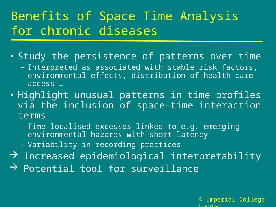
Benefits of Space Time Analysis for chronic diseases

• Study the persistence of patterns over time– Interpreted as associated with stable risk factors,

environmental effects, distribution of health care access …

• Highlight unusual patterns in time profiles via the inclusion of space-time interaction terms– Time localised excesses linked to e.g. emerging

environmental hazards with short latency– Variability in recording practices

Increased epidemiological interpretability Potential tool for surveillance


Joint analysis of two related chronic diseases or health outcomes is of interest in several contexts

• Epidemiology: quantify ‘expected’ variability linked to shared risk factors and tease out specific patterns

• Health planning: assess the performance of the health system, e.g. for health outcomes linked to screening policies

• Data quality issues: uncover anomalous patterns linked to a data source shared by several outcomes

Benefits of joint analysis of related diseases


Case study: Congenital anomalies in England

• All cases of congenital anomalies (non chromosomal) recorded in England for the period 1983 – 1998

• Data from national post-coded registers (Office for National Statistics)

• Annual post-coded data on total number of live births, still births and terminations

• 136,000 congenital anomalies 84.5 per 105 birth-years• Congenital anomalies are sparse:

Grid of 970 grid squares with variable size, to equalize the number of birth and expected cases per square

• Variations could be linked to socio-economic or environmental risk factors or heterogeneity in recording practises

Interest in characterising space time patterns© Imperial College London


Map of grid squares usedin the CongenitalAnomalies study



Annual expected0 - 2.5162.516 - 5.6475.647 - 9.5139.513 - 14.45914.459 - 64.087

Expected number of congenital anomalies per year in each square (per quintiles)

Annual expected

cong anomal.

Annual number of births

Min 0 0

20% 2.60 2994.8

40% 5.71 6576.2

Median

7.43 8569.0

60% 9.54 10994.6

80% 14.48 16687.4

Max 64.09 73872.0



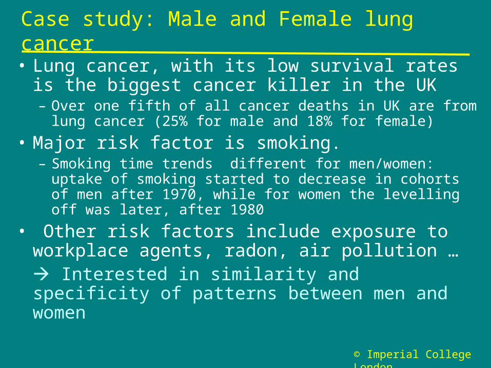
Case study: Male and Female lung cancer

• Lung cancer, with its low survival rates is the biggest cancer killer in the UK– Over one fifth of all cancer deaths in UK are from lung

cancer (25% for male and 18% for female)

• Major risk factor is smoking. – Smoking time trends different for men/women: uptake of

smoking started to decrease in cohorts of men after 1970, while for women the levelling off was later, after 1980

• Other risk factors include exposure to workplace agents, radon, air pollution … Interested in similarity and specificity of patterns between men and women


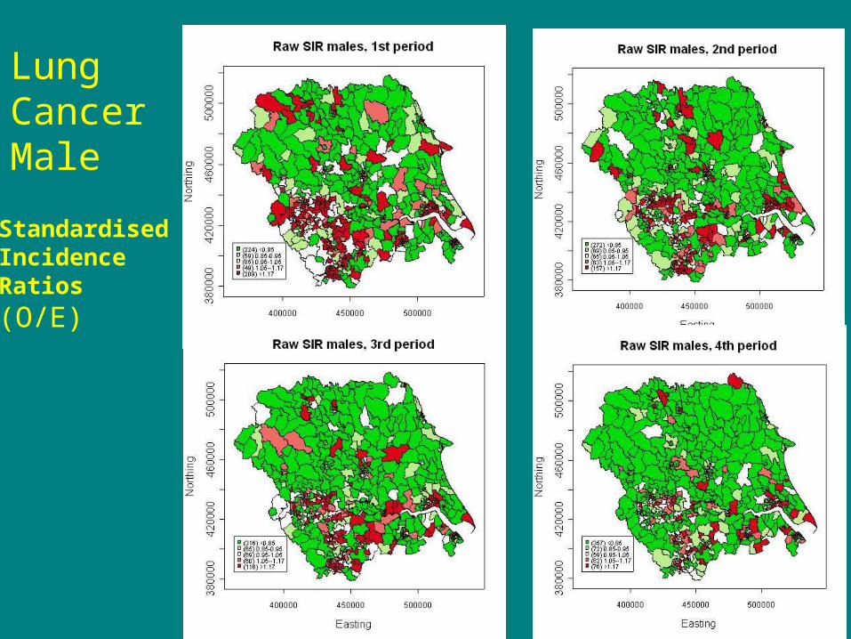
Data sets

• Female and Male lung cancer incidence in Yorkshire.

• Spatial resolution: wards (626): – between 0 and 20 new cases per year with mean

around 4 for male – between 0 and 12 per year with mean 1.8 for female

• Time periods: 1981-85, 1986-90, 1991-95, 1996-99.

• Expected counts based on sex-age incidence rates for the region and the total period 1981-1999


StandardisedIncidenceRatios

(O/E)

LungCancerMale


LungCancerFemale


Outline

• Context




• Discussion



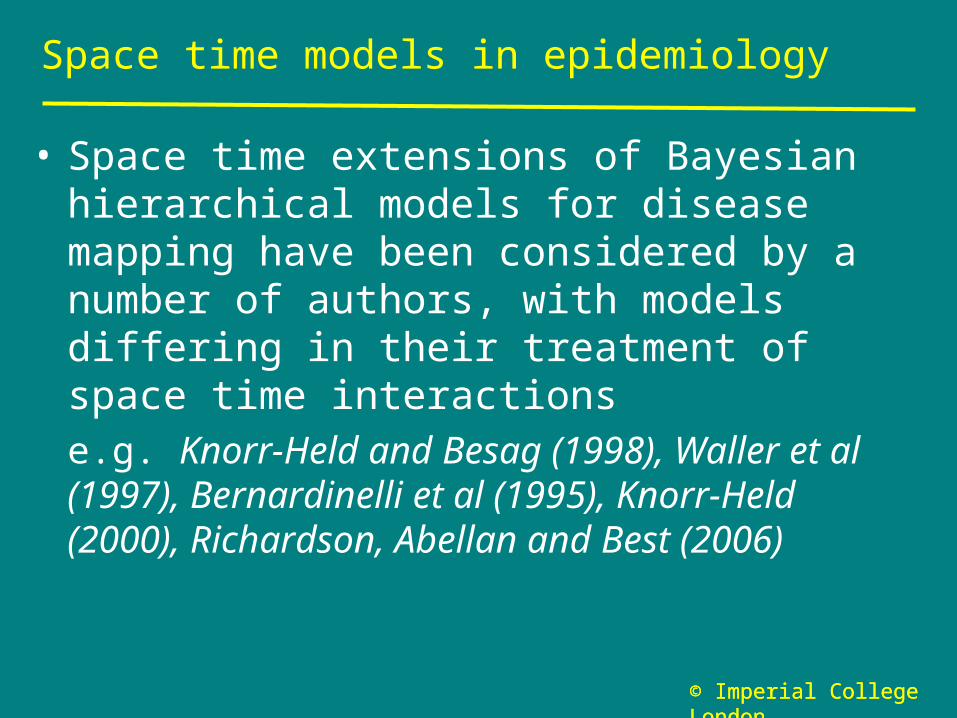
Space time models in epidemiology

• Space time extensions of Bayesian hierarchical models for disease mapping have been considered by a number of authors, with models differing in their treatment of space time interactionse.g. Knorr-Held and Besag (1998), Waller et al (1997), Bernardinelli et al (1995), Knorr-Held (2000), Richardson, Abellan and Best (2006)



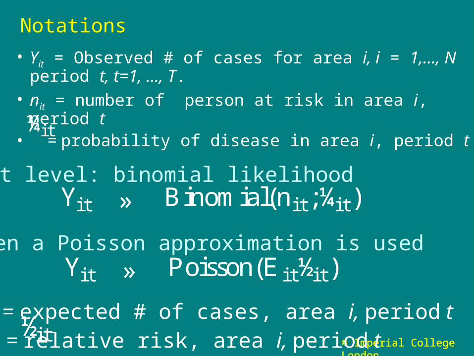
Notations

• Yit = Observed # of cases for area i, i = 1,…, N period t, t=1, …, T.

• nit = number of person at risk in area i, period t• = probability of disease in area i, period t

First level: binomial likelihood

¼i t

Often a Poisson approximation is used


Yi t » Binomial(ni t;¼i t)

Yi t » Poisson(E i t½i t)

Eit = expected # of cases, area i, period t = relative risk, area i, period t½i t


¼i t

Overall spatial pattern

Overall time trend

Space time interactions

Second level: modelling of the structure of the random effects or


½i t

µlogit(¼i t)log(½i t)

¶

= ®+ ¸ i + »t + ºi t

Prior structure for the random effects : • encodes prior epidemiological knowledge• need to borrow strength to effect smoothing• has to be adapted to the analysis’s aim


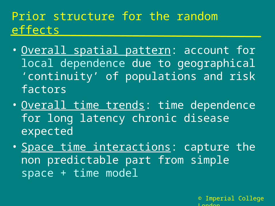
Prior structure for the random effects

• Overall spatial pattern: account for local dependence due to geographical ‘continuity’ of populations and risk factors

• Overall time trends: time dependence for long latency chronic disease expected

• Space time interactions: capture the non predictable part from simple space + time model


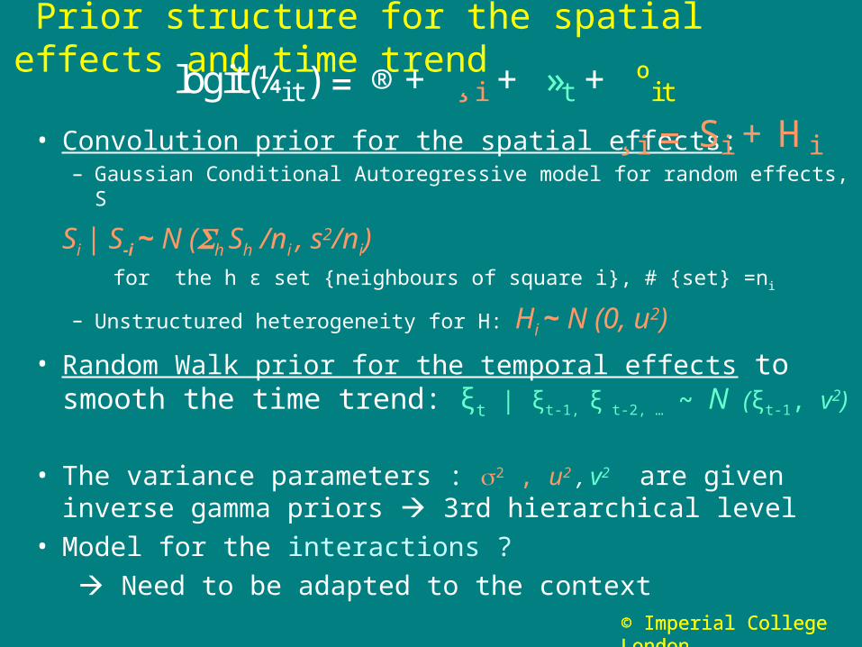
Prior structure for the spatial effects and time trend

• Convolution prior for the spatial effects: – Gaussian Conditional Autoregressive model for random effects, S

Si | S-i ~ N (h Sh /ni , s2/ni) for the h ε set {neighbours of square i}, # {set} =ni

– Unstructured heterogeneity for H: Hi ~ N (0, u2)

• Random Walk prior for the temporal effects to smooth the time trend: ξt | ξt-1, ξ t-2, … ~ N (ξt-1, v

2)

• The variance parameters : 2 , u2 , v2 are given inverse gamma priors 3rd hierarchical level

• Model for the interactions ?

Need to be adapted to the context

¸ i = Si + H i

logit(¼i t) = ®+ ¸ i + »t + ºi t



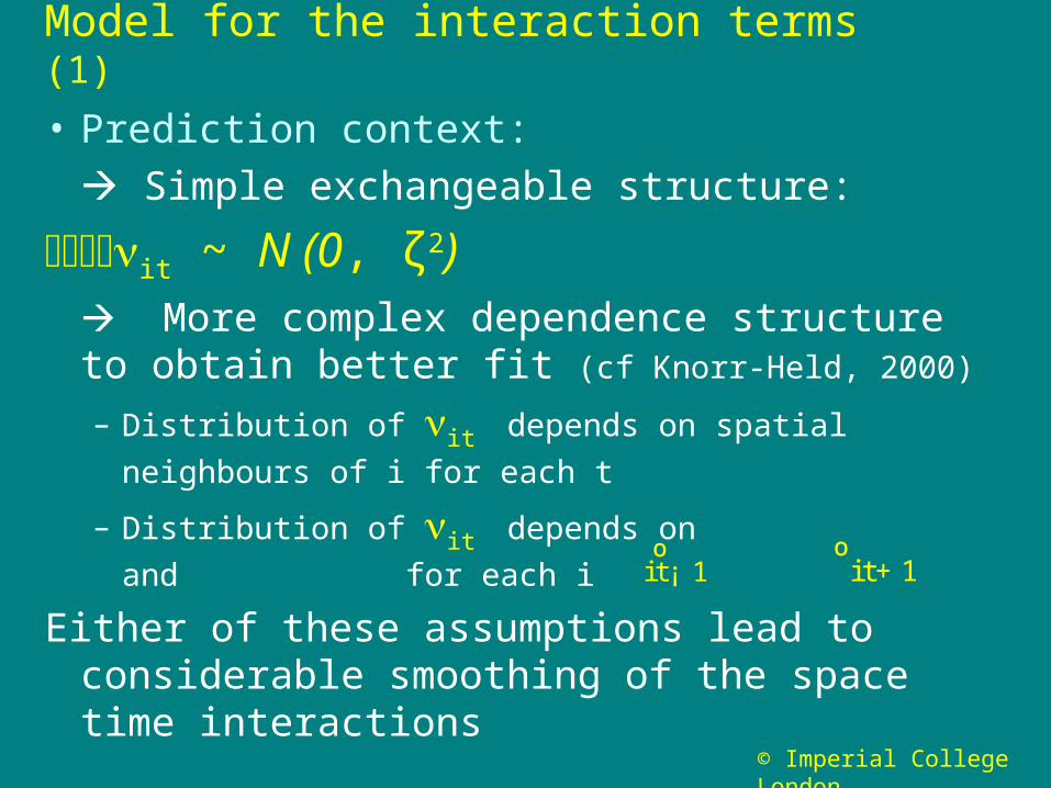
Model for the interaction terms (1)

• Prediction context:

Simple exchangeable structure:

it ~ N (0, ζ2) More complex dependence structure to obtain better fit (cf Knorr-Held, 2000)

– Distribution of it depends on spatial neighbours of i for

each t

– Distribution of it depends on and for

each i

Either of these assumptions lead to considerable smoothing of the space time interactions

ºi t¡ 1 ºi t+1


Model for the interaction terms (2)

• Investigating stability of patterns: Aim is to

-- Highlight true departures from the overall stable space + time model

-- Shrink idiosynchratic (non interpretable) interactions

Mixture model to characterise ‘stable’ and ‘unstable’ risk patterns over time

ºi t » pNormal(0;¿21) +(1¡ p)Normal(0;¿2

2 ):

¿2 » Normal(0;100) ¢I (0;+1 )

¿1 » Normal(0;0:01) ¢I (0;+1 )

Component 1 stable Component 2 unstable


Outline

• Context




• Discussion



Analysis strategy for investigating stability of patterns

• Estimate a model: space (CAR +Het) + time + interactions (mixture)• Use the posterior probabilities of allocation pit into

component 2 to classify areas as ‘unstable’• Rule: area i is unstable if at least for one t, 1, … T pit > pcut

(threshold probability)• For ‘stable’ areas, investigate spatial patterns, e.g. by

using the rule Prob(λi >1) > 0.8.

• Investigate the profile pattern of ‘unstable’ areas Need to evaluate the performance of the mixture model and associated classification rule


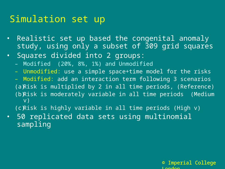
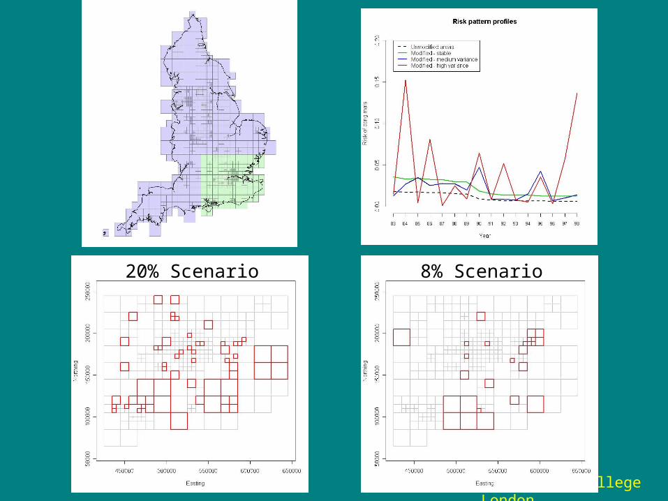
Simulation set up

• Realistic set up based the congenital anomaly study, using only a subset of 309 grid squares

• Squares divided into 2 groups:– Modified (20%, 8%, 1%) and Unmodified – Unmodified: use a simple space+time model for the risks– Modified: add an interaction term following 3 scenarios (a) Risk is multiplied by 2 in all time periods, (Reference) (b) Risk is moderately variable in all time periods (Medium v)(c) Risk is highly variable in all time periods (High v)

• 50 replicated data sets using multinomial sampling



20% Scenario 8% Scenario


Statistical issues

• If we over-fit, i.e. estimate a space-time model with interactions when the patterns are stable (Reference case), do we loose power to detect pure spatial patterns with respect to a pure spatial model ? :– Gain of interpretability but loss of power ?

• Is the mixture model identifiable ?• What is the performance of the classification rules ?• Can we tease out any structured patterns in the

interactions?



Comparison of the distribution of the {λi} and of the

posterior probabilities Prob(λi > 1) between the space time model and a pure spatial model fitted to the aggregate counts over the 16 years

Reference case


Variability of space-time interaction terms

• Compute the empirical standard deviation of the it , SD(it ) for each area (over the 16 years):

SD(it ) characterises the instability over time of the underlying disease risk

• Posterior distribution of SD(it ) is influenced overall– by the (unknown) proportion of areas with

unstable risks over time identified by the mixture– by the size of the interactions for the modified

areas



Posterior distribution of SD(it ) in the 3 casesMixture model

20% Modified areas 8% Modified areas 1% Modified areas

Model captures well the increased variability of modified areasClear distinction between medium and high variance cases Increasing number of modified areas influences overall fit


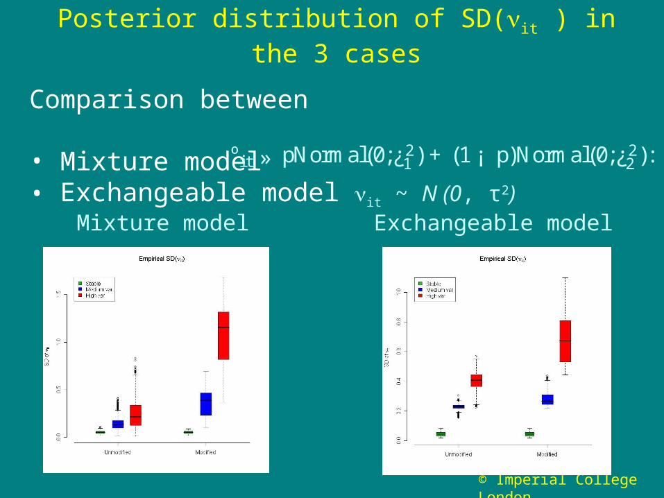
Posterior distribution of SD(it ) in the 3 cases

Comparison between

• Mixture model • Exchangeable model it ~ N (0, τ2)

ºi t » pNormal(0;¿21) +(1¡ p)Normal(0;¿2

2):

Mixture model Exchangeable model


Performance of Classification rule

Plot of sensitivity versus 1- specificity (ROC curves)Rule: area i is unstable if pit > pcut at least for one t, 1, … T For 90% specificity (10% False positive), pcut ≈ 0.5

20% Modified areas 8% Modified areas


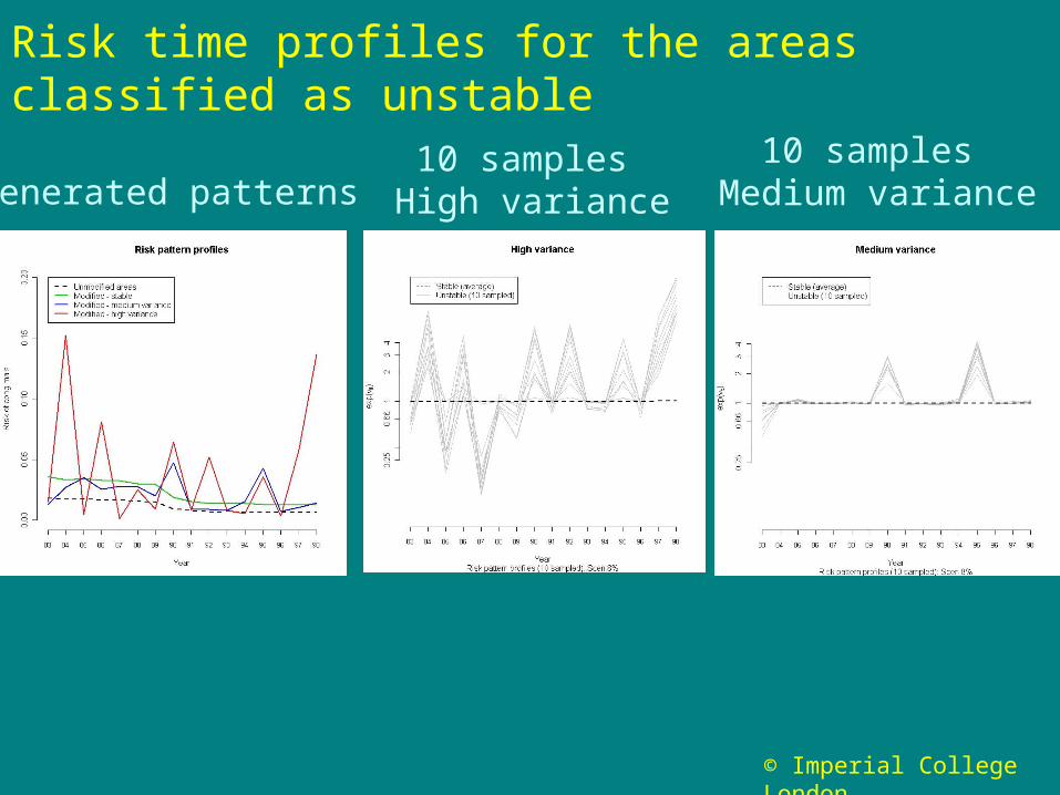
Risk time profiles for the areas classified as unstable

Generated patterns10 samples

High variance

10 samples Medium variance


Interpretation of excess risk in unmodified areas

Combining the rule Prob(λi > 1) > 0.8 and the classification rule is effective

• We found that for the unmodified areas generated with risk > 1.1: – 90% have Prob(λi > 1) > 0.8

– all are classified as stable

spatially stable excess risk better interpreted


Results for congenital anomalies

• Map of the global spatial pattern

• Time trend (83 - 98)

• Classification of areas

• Time profiles for unstable areas



Spatial main effect 970 grid squares

Post median of exp(λi)

Congenital anomalies England, 83-98


Evidence of spatial heterogeneity with higher risk in the North, NW and NE and in the Greater London area

Deprivation and maternal age are strong determinants of congenital malformations


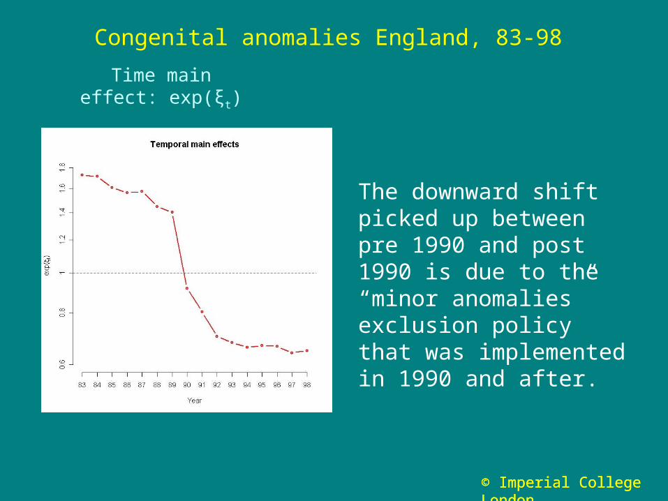
Time main effect: exp(ξt)

Congenital anomalies England, 83-98

The downward shift picked up between pre 1990 and post 1990 is due to the “minor anomalies”exclusion policy that was implemented in 1990 and after.



Mixture estimation

• Using a cut off pcut = 0.5, 125 areas are classified as unstable


Risk time profiles for the areas classified as unstable

We performed hierarchicalclustering on the 125 areas

Four subgroups exhibitsmooth-like trends interaction terms used toadjust to general time trend

One small subgroup has ahigh peak in 97 warrants investigation


Outline

• Context




• Discussion



Joint modelling of several diseases

• Spatial analysis of related diseases has been formulated in the BHM context by Knorr-Held and Best (2001)

• Extend the formulation of the shared component model to include a time dimension in order to study shared and specific patterns over time

• We shall formulate our models in the context of male and female lung cancer


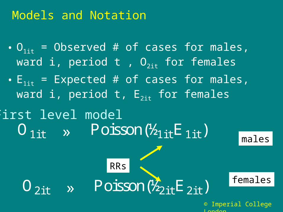
Models and Notation

• O1it = Observed # of cases for males, ward i, period t , O2it for females

• E1it = Expected # of cases for males, ward i, period t, E2it for females

First level model

RRs

males

females

O1i t » Poisson(½1i tE1i t)

O2it » Poisson(½2itE2it)


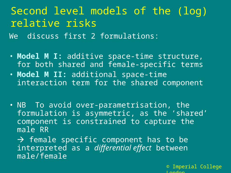
Second level models of the (log) relative risks

We discuss first 2 formulations:

• Model M I: additive space-time structure, for both shared and female-specific terms

• Model M II: additional space-time interaction term for the shared component

• NB To avoid over-parametrisation, the formulation is asymmetric, as the ‘shared’ component is constrained to capture the male RR female specific component has to be interpreted as a differential effect between male/female


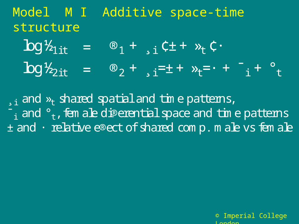
Model M I Additive space-time structure

log½1i t = ®1 + ¸ i ¢±+ »t ¢·

log½2i t = ®2 + ¸ i =±+ »t=· + ¯ i + °t

¸ i and »t shared spatial and time patterns,¯ i and °t, female di®erential space and time patterns±and · relative e®ect of shared comp. male vs female


Model M II ‘Common’ space-time interaction

Inclusion of terms it

investigate common pattern of departure from a simple additive space time structure

log½1i t = ®1 + ¸ i ¢±+ »t ¢· + ºi t

log½2i t = ®2 + ¸ i =±+ »t=· + ºi t + ¯ i + °t

Does the share term it captures all the local space-time patterns ?


log½1i t = ®1 +¸ i ¢±+»t ¢· +ºi t +Á1i t

log½2i t = ®2 +¸ i =±+ »t =· +ºi t +¯ i +°t + Á2i t

log½1it = ®1 +¸ i ¢±+»t ¢· + Á1i t

log½2it = ®2 +¸ i =±+»t =· +¯ i +°t + Á2i t

Explore benefit of additional male and female specific residual terms in Model I or II

Model M II + het

Model M I + het


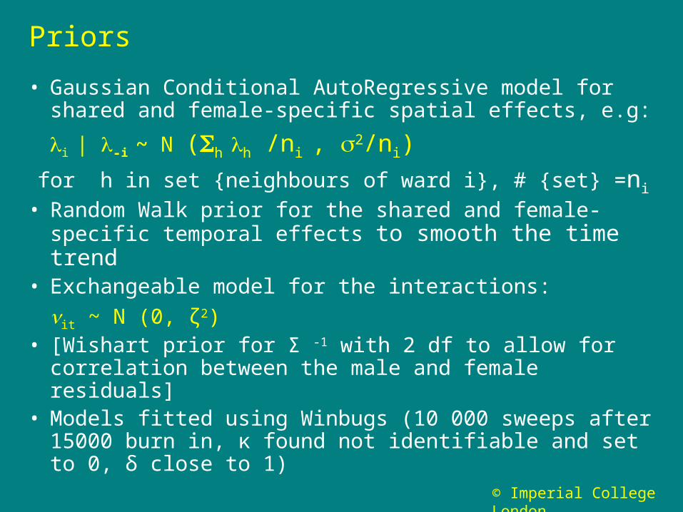
Priors

• Gaussian Conditional AutoRegressive model for shared and female-specific spatial effects, e.g:

i | -i ~ N (h h /ni , 2/ni)

for h in set {neighbours of ward i}, # {set} =ni

• Random Walk prior for the shared and female-specific temporal effects to smooth the time trend

• Exchangeable model for the interactions:

it ~ N (0, ζ2)• [Wishart prior for Σ -1 with 2 df to allow for correlation

between the male and female residuals] • Models fitted using Winbugs (10 000 sweeps after

15000 burn in, κ found not identifiable and set to 0, δ close to 1)


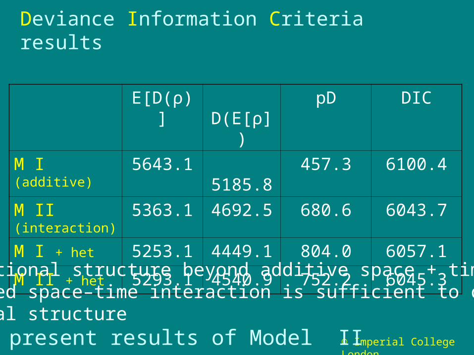
Deviance Information Criteria results

E[D(ρ)] D(E[ρ])

pD DIC

M I (additive) 5643.1 5185.8 457.3 6100.4

M II (interaction) 5363.1 4692.5 680.6 6043.7

M I + het 5253.1 4449.1 804.0 6057.1

M II + het 5293.1 4540.9 752.2 6045.3

• Additional structure beyond additive space + time?• Shared space–time interaction is sufficient to captureresidual structure

present results of Model II


Results for Model II

• Smoothed relative risks for male and female

• Shared and female specific spatial patterns

• Time trends

• Posterior probabilities for space-time interaction terms


RR Male 1st period RR Male 2nd period

RR Male 3rd period RR Male 4th period


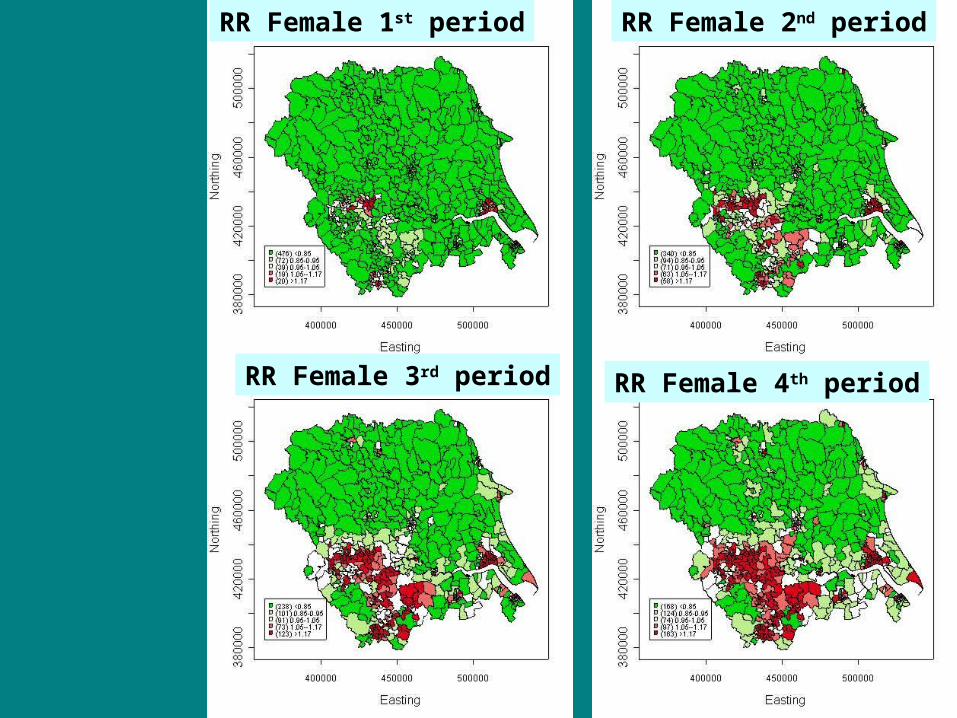
RR Female 1st period RR Female 2nd period

RR Female 4th periodRR Female 3rd period


Comments

Maps of smoothed RRs show:

• Evidence of spatial heterogeneity with higher RR in urban areas in the SW: Leeds, Bradford, Huddersfield, Sheffield, and towards Hull

• Opposite time trends in male and female– Decrease over time period for male– Increase over the period for female

Characterisation of these components


Posterior prob that βi > 1

Shared component Specific female component

Higher male/femaledifferential in extendedsemi rural area north of Leeds

Clear urban/rural differences in incidence. Linked to smoking patterns? Air pollution?


10 wards selected at random

Time trends, male in red, female in blue

Time trend for male RRsin 10 wards

Time trend for female RRsin 10 wards

Differential time trends are linked to lagged uptake of smoking in cohorts of men and women


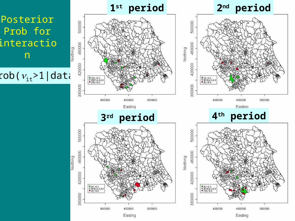
Model II + ‘Common’ interactions

• ‘High’ values of interaction terms it indicate a lack of fit of the simple additive formulation of model I : space x time space + time for the shared part

• Here we did not use a mixture model but a simple exchangeable model

• More informative than the display of posterior mean estimates for the terms it , display of the

posterior probabilities, Prob(it > 1)


Prob(it>1|data)

PosteriorProb for

interaction

2nd period

4th period

1st period

3rd period


Model II

• Interactions seem predominant in the SW corner

• Number of areas highlighted are compatible with expected number of false positives

• For long latency disease like lung cancer, epidemiological patterns tend to be stable

• Explore link between shared structure and contextual covariates

Standardise the expected counts Eit with respect to deprivation index and re-estimate Model II


Sharedpattern becomes weaker indicating link to deprivation

Female differential stays similar


Discussion (1)

• Bayesian space time analyses allow a richer interpretation of patterns than purely spatial ones

• Models become more complex, with more choice of prior structure : in particular, the prior structure for the space time interactions (t distribution, semi-parametric mixture, other smoothing priors ….) Need to think of prior structure in relation to the different

aims of the analyses, the time scale and the hypotheses on the health phenomenon under investigation

sensitivity analyses and careful exploration of models is needed



Discussion (2)

• To gain epidemiologic interpretability, the stability = repeatability over time of spatial patterns found by a pure spatial analysis should be investigated little loss of power to detect areas with increased risk

decision rules that discriminate between stable and unstable patterns based on mixture model seem promising

• Need to investigate the effect of a smaller number of expected events (in our simulations, median per area between 4 and 9 in different years)



Discussion (3)

• How to explore further the pattern showed by the space-time interactions ?

• Investigate generalisation of the hierarchical clustering to more flexible clustering of time profiles of space-time interactions, e.g. in a Bayesian hierarchical framework, to better detect structured patterns in the time profiles of risks

• Comparison with other methods for finding space-time clusters (e.g. Scan statistics)


References

• L. Bernardinelli, D. Clayton, C. Pascutto, C. Montomoli, M. Ghislandi, and M. Songini. Bayesian. Analysis of space-time variation in disease risk. Statistics in Medicine, 14:2433–2443, 1995.

• L. A. Waller, B. P. Carlin, H. Xia, and A. M. Gelfand. Hierarchical spatio-temporal mapping of disease rates. Journal of the American Statistical Association, 92:607–617, 1997.

• L. Knorr-Held and J. Besag. Modelling risk from a disease in time and space. Statistics in Medicine, 17:2045–2060, 1998.

• L. Knorr-Held. Bayesian modelling of inseparable space-time variation in disease risk. Statistics in Medicine, 19:2555–2567, 2000.

• L. Knorr-Held and N. G. Best. A shared component model for detecting joint and selective clustering of two diseases. Journal of the Royal Statistical Society - A, 164:73–85, 2001.

• S. Richardson, J. J. Abellan, and N. Best. Bayesian spatio-temporal analysis of joint patterns of male and female lung cancer risks in Yorkshire (UK). Statistical Methods in Medical Research, 15: 385-407, 2006.

• J. J. Abellan, S. Richardson, and N. Best. Use of space-time models to investigate the stability of patterns of disease. (2007). Submitted for publication.

© imperial college london analysis of space time patterns of disease risk sylvia richardson centre...

Documents

time profiles

public health slide

health outcomes

cases of congenital

environmental risk factors

female lung cancer lung

surveillance slide

shared risk factors