circabc.europa.eu · web viewenvironmental quality standard. a term most often used in reference to...

SUPPLEMENTARY GUIDANCE FOR THE IMPLEMENTATION OF EQSBIOTA

Final Draft

Disclaimer:

This technical document has been developed by a drafting group through a collaborative programme involving the European Commission, Member States, Switzerland, and other stakeholders. The document does not necessarily represent the official, formal position of any of the partners. Hence, the views expressed in the document do not necessarily represent the views of the European Commission.

i

FOREWORDTo be completed.

ii

CONTENTSFOREWORD............................................................................................................ iiCONTENTS............................................................................................................. iiiTABLES................................................................................................................... vFIGURES................................................................................................................ viGLOSSARY OF TERMS...........................................................................................vii1 INTRODUCTION...............................................................................................1

1.1 Background..............................................................................................11.2 Aims.........................................................................................................11.3 Scope and structure.................................................................................21.4 Protection goals of biota EQS...................................................................3

1.4.1 Chemicals for which there is currently an EQSbiota................................31.5 Other relevant EU legislation...................................................................5

2 KEY CHALLENGES IN IMPLEMENTING BIOTA STANDARDS...............................62.1 Expression of biota standards..................................................................6

2.1.1 Summary statistic.................................................................................62.1.2 Period over which the standard applies................................................7

2.2 Species to be sampled.............................................................................83. HOW TO USE THIS GUIDANCE.........................................................................9

3.1 Identifying sampling locations.................................................................93.2 Designing the sampling programme........................................................93.3 Selecting a suitable matrix....................................................................103.4 Data handling........................................................................................103.5 Assessing Compliance............................................................................10

4. IDENTIFYING SAMPLING LOCATIONS AND DESIGNING THE SAMPLING PROGRAMME........................................................................................................11

4.1 Conceptual Model..................................................................................114.2 Design of a sampling programme..........................................................12

4.2.1 How many samples are needed?........................................................134.2.2 How much tissue is needed?..............................................................14

5. SELECTING A SUITABLE MATRIX....................................................................165.1 Wild-caught biota (passive biomonitoring).............................................17

5.1.1 Selection of species............................................................................175.1.2 Minimising natural variability.............................................................18

5.1.2.1 Age and size...............................................................................185.1.2.2 Migration behaviour....................................................................195.1.2.3 Condition factor..........................................................................195.1.2.4 Gender........................................................................................205.1.2.5 Seasonality.................................................................................205.1.2.6 Stocked versus indigenous populations......................................21

5.2 Caged biota (active biomonitoring)........................................................225.2.1 Species selection................................................................................225.2.2 Minimising variability..........................................................................225.2.3 Caging systems..................................................................................235.2.4 Duration and timing of deployment....................................................24

5.3 Choice of tissue for contaminant analysis..............................................255.3.1 Current practice from ongoing monitoring programmes....................255.3.2 Implications of using whole fish versus fish tissues/ organs when assessing compliance...................................................................................30

6. DATA HANDLING...........................................................................................356.1 Lipid and dry weight normalisation........................................................356.2 Trophic Level..........................................................................................36

iii

7. ASSESSING COMPLIANCE WITH A BIOTA EQS...............................................387.1 Using measured chemical concentrations to determine compliance.....387.2 Estimating confidence in compliance assessments...............................397.3 Assessment period.................................................................................40

ANNEXES.............................................................................................................41A.1 Steps applied for the selection of biota for a monitoring programme in France (2011-2013)..........................................................................................41

A.1.1 Background.......................................................................................41A.1.2 Step 1: Accumulation potential.........................................................41A.1.3 Step 2: Matching the accumulation potential with fish availability...41A.1.4 Step 3: Species selection..................................................................42A.1.5 Step 4: Feasibility check...................................................................42

A.2 Using trend monitoring data to assess EQS compliance........................44A.3 Screening as an approach to developing a biota monitoring programme

47A.3.1 Water................................................................................................47A.3.2 Suspended matter............................................................................47A.3.3 Sediment..........................................................................................48A.3.4 Passive sampling..............................................................................48A.3.5 Models..............................................................................................48A.3.6 Conclusion........................................................................................49

A.4 Potential use of passive sampling..........................................................50A.4.1 Example of monitoring by passive sampling in concert with deployed mussels.........................................................................................................51

A.5 Quantity and preparation of biological material required for contaminant analyses...........................................................................................................54

A.5.1 Quantity of biological material required for analysis........................54A.5.2 Preparation of samples for whole body analysis (small fish and invertebrates)...............................................................................................57A.5.3 Preparation of tissue samples (big invertebrates and fish)...............58

A.6 Estimating whole fish contaminant concentrations from tissue concentrations.................................................................................................59

A.6.1 An example of a method to develop equations for the estimation of whole-fish contaminant concentrations (excerpt from Bevelhimer et al. 1997)

59A.6.2 Limitations and uncertainties to be considered................................60

A.7 Normalisation of measured data............................................................62A.8 Trophic Level determination..................................................................63A.9 Trophic level conversion........................................................................64A.10 Members of the expert drafting group...................................................65

REFERENCES........................................................................................................67

iv

TABLESTable 1.1 Current EQSbiota and basis for derivation...............................................4Table 5.1 Advantages and limitations of passive and active monitoring (Besse et al. 2012) ...............................................................................................................

16Table 5.2 Species/tissues used currently in European biota monitoring programmes........................................................................................................27Table 5.3 Biota quality standards (QSbiota) derived for the two different protection goals. 31Table 5.4 Tissues/ organs in which contaminants can be measured in fish.......33Table A.1.1 Most frequently sampled species in France (2011-2013)..............42Table A.1.2 Species, sample size and mass scenarios......................................43Table A.5.1 Tissue weight requirements for contaminant analyses specified in

monitoring programmes using biota for pollution assessment......54

v

FIGURESFigure 3.1 Steps that must considered when designing and implementing a

sampling campaign to assess status with respect to biota standards 9Figure 4.1 Power analysis relating sample number and confidence in decision making. 14Figure A.1.1 Maps showing the sites matching the project criteria...................43Figure A.2.1 Time series of Hg concentrations in Perch from Lake Bysjön........45Figure A.2.2 Time series of Hg concentrations in arctic char from Lake Abiskojaure. 46Figure A.4.1 A time series of Fluoranthene concentrations in the mid Western

Scheldt for mussels.......................................................................52Figure A.4.2 A time series of PCB153 concentrations in the west Wadden Sea.53Figure A.6.1 Flow diagram describing statistical procedures used to determine

equations for estimating fish contaminant concentrations from fillet values (redrawn from Bevelhimer et al. 1997)..............................61

vi

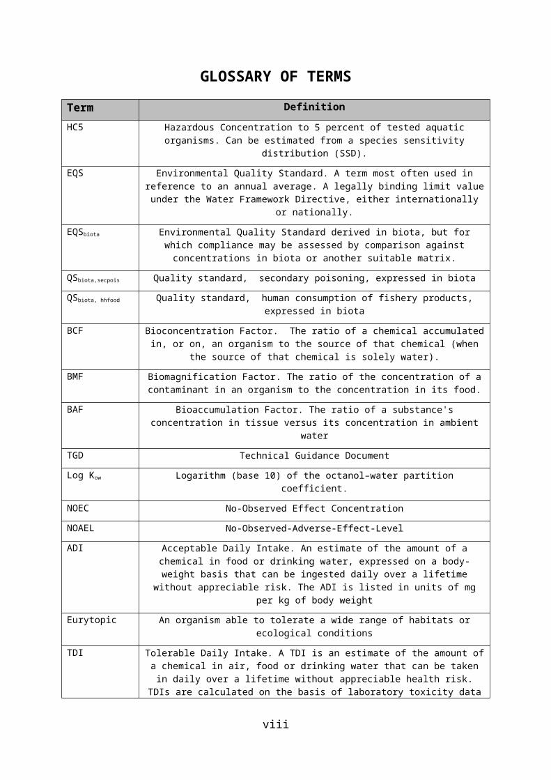
GLOSSARY OF TERMSTerm DefinitionHC5 Hazardous Concentration to 5 percent of tested aquatic organisms. Can

be estimated from a species sensitivity distribution (SSD).EQS Environmental Quality Standard. A term most often used in reference to

an annual average. A legally binding limit value under the Water Framework Directive, either internationally or nationally.

EQSbiota Environmental Quality Standard derived in biota, but for which compliance may be assessed by comparison against concentrations in

biota or another suitable matrix.QSbiota,secpois Quality standard, secondary poisoning, expressed in biotaQSbiota, hhfood Quality standard, human consumption of fishery products, expressed in

biotaBCF Bioconcentration Factor. The ratio of a chemical accumulated in, or on,

an organism to the source of that chemical (when the source of that chemical is solely water).

BMF Biomagnification Factor. The ratio of the concentration of a contaminant in an organism to the concentration in its food.

BAF Bioaccumulation Factor. The ratio of a substance's concentration in tissue versus its concentration in ambient water

TGD Technical Guidance DocumentLog Kow Logarithm (base 10) of the octanol–water partition coefficient.NOEC No-Observed Effect ConcentrationNOAEL No-Observed-Adverse-Effect-LevelADI Acceptable Daily Intake. An estimate of the amount of a chemical in food

or drinking water, expressed on a body-weight basis that can be ingested daily over a lifetime without appreciable risk. The ADI is listed

in units of mg per kg of body weightEurytopic An organism able to tolerate a wide range of habitats or ecological

conditionsTDI Tolerable Daily Intake. A TDI is an estimate of the amount of a chemical

in air, food or drinking water that can be taken in daily over a lifetime without appreciable health risk. TDIs are calculated on the basis of laboratory toxicity data to which uncertainty factors are applied.

TMF Trophic Magnification FactorCF Condition FactorJAMP Joint Assessment and Monitoring ProgrammePFOS Perfluorooctanesulfonic acid or perfluorooctane sulfonate

vii

LOQ Limit of Quantification.DDT DichlorodiphenyltrichloroethanePBDEs Polybrominated Diphenyl EthersBFR Brominated Flame RetardantPCDD/F Polychlorinated Dibenzo-p-Dioxin and Polychlorinated DibenzofuranPFAAs Perfluoroalkyl AcidsPAH Polycyclic Aromatic HydrocarbonHCB HexachlorobenzeneHCBD HexachlorobutadieneNDL-PCB

DL-PCB

Non-Dioxin-like Polychlorinated BiphenylDioxin-like Polychlorinated Biphenyl

HBCDD HexabromocyclododecaneVOCs Volatile Organic CompoundsPOPs Persistent Organic PollutantsVSD Virtual Safe DosePCB-7 2,4-Dichlorobiphenyl

viii

1 INTRODUCTION1.1 BackgroundThe 2013 European Commission Directive dealing with Priority Substances under the Water Framework Directive (2013/39/EC) amends and updates the original Water Framework and Environmental Quality Standard (EQS) Directives (EC 2000 and EC 2008, respectively). As well as adding new substances and updating surface water EQS, the new Directive adds (for 8 substances) an EQSbiota. For 5 of these substances an EQSwater is also included. Member States (MS) will need to establish programmes to monitor the concentration of substances in biota or water and assess compliance against new standards.

The biota standards refer to fish, except in the case of PAHs and fluoranthene, where reference is made to fish, crustaceans and molluscs (consistent with the food safety legislation). According to Article 3.3 of the Directive 2013/39/EU (EC 2013), Member States may opt, in relation to one or more categories of surface water, to apply an EQS for a matrix other than that specified in article 3.2, or, where relevant, for a biota taxon other than those specified in Part A of Annex I. Where an EQS has been set for biota, an equivalent standard can be derived for the water column (using the Bioconcentration Factor (BCF)/ Biomagnification Factor (BMF) or Bioaccumulation Factor (BAF)). However, the measurement of these chemicals in the water column at the resulting extremely low concentrations can be analytically very challenging. Nevertheless, it is a MS decision as to which matrix is used for compliance assessment as there are a range of practical and ethical issues to be considered if biota sampling is the chosen matrix.

1.2 AimsExisting EU-wide guidance effectively addresses the derivation of EQSbiota (EC 2011a), but not how to implement the standards. CIS Guidance 25 (EC 2010) addresses some of the questions but does not cover how the results derived from such monitoring programmes are used to assess compliance with the EQSbiota. Without additional guidance, different approaches are likely to be adopted by different Member States, and the resulting data will lack consistency, prevent an EU-wide assessment of compliance with the biota standards and will result in a fragmented and unreliable view with respect to the actual pressures posed by bioaccumulative substances.

This document aims to promote consistency in the implementation of biota standards by providing supplementary guidance on the design and implementation of biota monitoring programmes. It covers the design of biota monitoring programmes, collection of samples, processing and expression of data, and explains how such data are then used to undertake compliance assessments.

1

The main objective of the supplementary guidance is therefore to provide practical guidance, specifically recommendations for the implementation of biota-related Water Framework Directive requirements in the Member States. This will help to ensure consistency and comparability between Member States when assessing compliance against EQSbiota.

1.3 Scope and structureThe guidance provided in this document is intended to be:

Specific and detailed, providing clear recommendations in areas which are dealt with in a generic manner by the existing guidance;

Objective and based on the current scientific evidence;

Technical, rather than policy-based; and,

Based on highlighted examples of existing schemes or systems that meet specific aspects of the implementation of EQSbiota.

It also highlights uncertainties in the recommended approaches where appropriate.

It is not intended to:

Reconsider or revisit the derivation of the EQSbiota (other than outlining the process for reference purposes);

Provide any methodology for the preparation, extraction or chemical analysis of biota samples;

Invalidate existing long-term programmes of biota monitoring which were designed to assess trends in substance concentrations (while such programmes may also be useful in assessing compliance with EQSbiota, they made require modification going forward to ensure the reliable delivery of both objectives).

Importantly, every effort has been made to produce guidance that reflects best practice in the design and execution of biota monitoring exercises.

The supplementary guidance covers three main areas:

Key challenges in implementing biota standards (Section 2);

Guidance on designing a sampling program and selecting a suitable matrix (Sections 4 and 5); and,

Data handling and assessing compliance with the EQSbiota (Sections 6 and 7).

2

Annexes provide supporting information to be used in designing and implementing biota monitoring programmes, such as cross-cutting issues between compliance monitoring and trend monitoring, tiered approaches, the use of passive samplers, tissue requirements for chemical assessments, as well as some examples of existing biota monitoring programmes.

3

1.4 Protection goals of biota EQSEQS should protect freshwater and marine ecosystems from the potential adverse effects of chemicals, as well as protecting human health from adverse effects via drinking water or the intake of food originating from aquatic environments. Several different protection goals were therefore considered in the derivation of EQS, i.e. the pelagic and benthic communities in freshwater, brackish and marine ecosystems, the predators of these ecosystems, and human health. Not all protection goals need to be considered for every substance. However, where a possible risk was identified, quality standards were derived for that protection goal.

EQSbiota have two protection goals:

Protection from chemical accumulation in the food chain, specifically of top predators such as birds and mammals, from risks of secondary poisoning through consumption of contaminated prey (referred to in the guidance as QSbiota,secpois);

Protection of human health from deleterious effects resulting from the consumption of food (fish, molluscs, crustaceans, oils, etc.) contaminated by chemicals (referred to in the guidance as QSbiota, hhfood).

In the EQS Technical Guidance Document (TGD) (EC 2011b) it is stressed that biota standards developed for birds and mammals are assumed to also be protective for benthic and pelagic predators. Importantly, the EQS is always based on the most stringent QS from the assessment, so compliance with an EQS will automatically mean that other receptors are protected, even if they are not explicitly addressed in the EQS.

The selection of sampling sites, the selection of the species to be monitored, the size of the organisms and the tissue to be analysed may be controlled by the protection goal of the biota standard. Hence, recommendations given in the following chapters take account of the relevant protection goal of the EQSbiota

where necessary.

1.4.1 Chemicals for which there is currently an EQSbiota

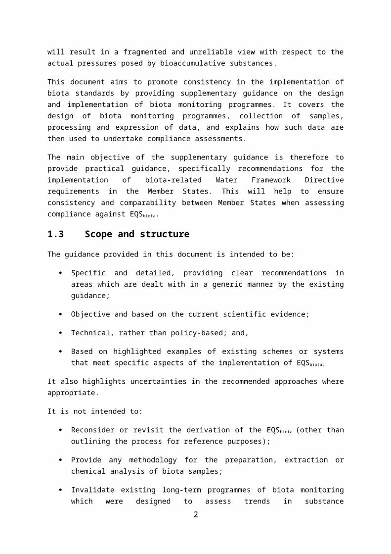
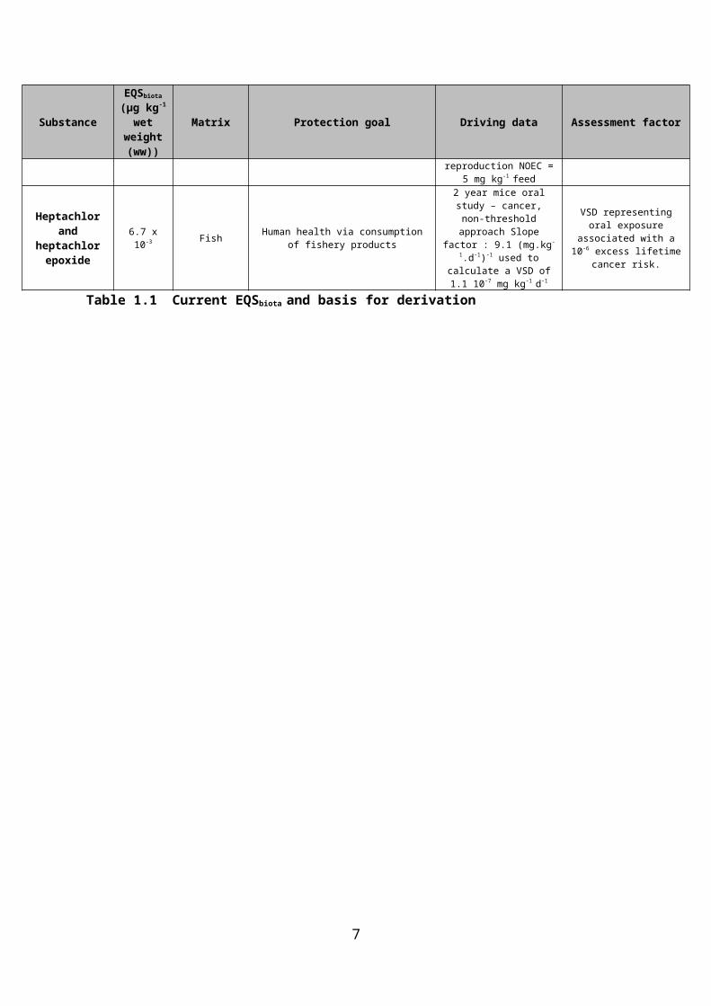
There are currently 11 chemicals or chemical groups for which EQSbiota have been derived. These are shown in Table 1.1, along with the matrix to which the EQS applies, on, the protection goal, the driving data and the assessment factor used.

As can be seen from the table, the majority of the chemicals have EQSbiota

derived for prey items (food) that are described as ‘fish’. The exceptions are for the PAHs for which crustaceans and molluscs are listed.

4

Substance

EQSbiota

(μg kg-1

wet weight (ww))

Matrix Protection goal Driving data Assessment factor

Brominated diphenyl ethers

0.0085 Fish Human health via consumption of fishery products

Mice dietary toxicity BMDL10

for BDE-99 = 9 μg kg-1

bw = internal daily dose of 4.2 ng kg-1

bw d-1 (using longest human half-life (1442 days)

30

Fluoranthene 30 Crustaceans and molluscs

Human health via consumption of fishery products

0.2 mg.kg-1 d-1, chronic oral (gavage) rat study used to

calculate a virtually safe dose (VSD) of 5x10-4 mg kg-1 d-1.

VSD representing oral exposure associated with a 10-6 excess lifetime cancer

risk based on the read-across between benzo[a]pyrene

and fluoranthene

Hexachloro-benzene

10 Fish Human health via consumption of fishery products

WHO-EHC guidance value for neoplastic effects of 0.16 μg

kg bw-1 d-1

Based on a person weighing 70 kg

(acceptable daily intake of 1.12 μg hexachlorobenzene

d-1) and an average fish consumption of 115 g d-1

Hexachloro-butadiene

55 Fish Secondary poisoning Chronic NOAEL mice = 0.2 mg kg-1 bw d-1

Conversion factor = 8.3 (kg bw.kg food-1.d-1) = 1.66 mg

kg food-1

Assessment factor = 30

Mercury and its compounds

20 Fish Secondary poisoning365 day NOEC rhesus

monkey growth 0.22 mg kg-1

food

10 , due to the large number of NOECs available for

methyl mercury

PAHsBenzo[a]pyrene

5 Crustaceans and molluscs


Maximum levels for foodstuffs for

benzo[a]pyrene:- 0.005 mg.kg-1

ww for crustaceans and molluscs

Maximum levels given for “fresh” (other than smoked)

aquatic resources. No assessment factor applied.

Dicofol 33 Fish Secondary poisoning

Falco sparverius Reproduction

NOEC = 1 mg kg-1

feed ww

30

PFOS 9.1 Fish Human health via consumption of fisheryproducts

Cynomolgus monkey183d NOAEL = 0.03 mg kg-1 90

Dioxins and dioxin-like

compounds

0.0065 TEQ2005

Fish, crustaceans and

molluscs


Maximum levels given for foodstuffs content of the

sum of DL-compounds(PCDDs, PCDFs and DL-PCBs)

HBCDD 167 Fish Secondary poisoning Japanese Quail reproduction NOEC = 5 mg kg-1 feed 30

Heptachlor and heptachlor

epoxide6.7 x 10-3 Fish Human health via consumption of fishery

products

2 year mice oral study – cancer, non-threshold

approach Slope factor : 9.1 (mg.kg-1.d-1)-1 used to

calculate a VSD of1.1 10-7 mg kg-1 d-1

VSD representing oral exposure associated with a 10-6 excess lifetime cancer

risk.

Table 1.1 Current EQSbiota and basis for derivation

5

1.5 Other relevant EU legislationRegulation (EC) No 315/93 established the principle that maximum levels should be set for contaminants in foodstuffs in order to protect public health, and Commission Regulation (EEC) No 1881/2006 then established levels for a number of contaminants in marine or freshwater food (amended by Commission Regulations, 420/2011, 835/2011, 1259/2011 amending regulation No 1881/2006). The contaminants that are currently covered under the European food regulations that are relevant to fish, shellfish and fish-related products (such as fish oils) include mercury, lead, cadmium, PCBs, dioxins and dioxin-like PCBs, and PAHs.

The levels in fish and fishery products are set on the basis of European Food Safety Authority (EFSA) advice and are given as tolerable weekly intakes in micrograms per kilogram body weight and maximum levels in foodstuffs (specifically relevant is the edible part of the foodstuffs in relation to fish and shellfish). For example, the limit for mercury is 0.5 mg kg -1 wet weight (ww) crustaceans and some fish, and 1.0 mg kg-1 ww for some specific fishes (mainly large), and for the sum of dioxins and dioxin-like PCBs it is 6.5 pg g -1 ww (WHOPCDD/ F-PCB-TEQ) for ‘seafood’, except eel for which the value is 10 pg g -1

ww (TEQ2005). Benzo[a]pyrene and PAH4 (the sum of benzo[a]pyrene, benz[a]anthracene, benzo[b]fluoranthene and chrysene) are used as markers for the occurrence and effect of carcinogenic PAHs in food. The limits for bivalves are 5.0 µg kg-1 and 30 µg kg-1 for BaP and PAH4, respectively.

6

2 KEY CHALLENGES IN IMPLEMENTING BIOTA STANDARDS

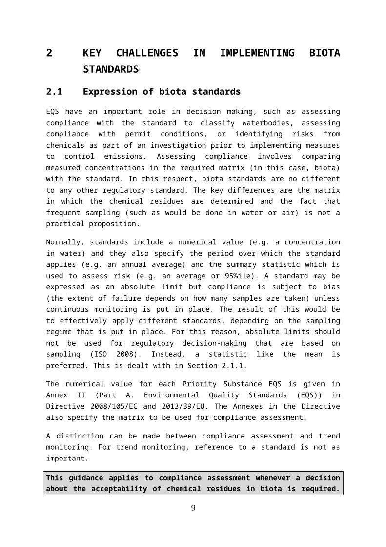
2.1 Expression of biota standardsEQS have an important role in decision making, such as assessing compliance with the standard to classify waterbodies, assessing compliance with permit conditions, or identifying risks from chemicals as part of an investigation prior to implementing measures to control emissions. Assessing compliance involves comparing measured concentrations in the required matrix (in this case, biota) with the standard. In this respect, biota standards are no different to any other regulatory standard. The key differences are the matrix in which the chemical residues are determined and the fact that frequent sampling (such as would be done in water or air) is not a practical proposition.

Normally, standards include a numerical value (e.g. a concentration in water) and they also specify the period over which the standard applies (e.g. an annual average) and the summary statistic which is used to assess risk (e.g. an average or 95%ile). A standard may be expressed as an absolute limit but compliance is subject to bias (the extent of failure depends on how many samples are taken) unless continuous monitoring is put in place. The result of this would be to effectively apply different standards, depending on the sampling regime that is put in place. For this reason, absolute limits should not be used for regulatory decision-making that are based on sampling (ISO 2008). Instead, a statistic like the mean is preferred. This is dealt with in Section 2.1.1.

The numerical value for each Priority Substance EQS is given in Annex II (Part A: Environmental Quality Standards (EQS)) in Directive 2008/105/EC and 2013/39/EU. The Annexes in the Directive also specify the matrix to be used for compliance assessment.

A distinction can be made between compliance assessment and trend monitoring. For trend monitoring, reference to a standard is not as important.

This guidance applies to compliance assessment whenever a decision about the acceptability of chemical residues in biota is required. This is a key driver for classification and it may also be required when biota standards are used as part of investigative monitoring.

2.1.1 Summary statistic

Concentrations of priority substances in biota typically have a log-normal distribution. An estimate of the central tendency, like a mean or median is therefore appropriate. For simplicity and consistency, the mean of the log-transformed data is the summary statistic to be used in decision-making.

The most reliable summary statistic (for comparison with an EQSbiota) is therefore the mean of log-transformed measured concentrations, after

7

normalisation as described in Section 6.1, collected from individual samples1.

2.1.2 Period over which the standard applies

Chemical residues found in biota will reflect their exposure to bio-accumulating chemicals over a period of time2. Because analysis of biota provides an integrated measure of the water column/sediment conditions they have been exposed to, it is theoretically possible to monitor less frequently than is needed for sampling a more mobile medium, like water. This assumes that samples taken on one occasion in a year are representative of samples taken at any other time. This is also related to the assumption that the kinetics of uptake and elimination in the chosen species is sufficiently slow to prevent rapid concentration changes, which are dependent on both the bioaccumulation potential of the substance and the size of the organism.

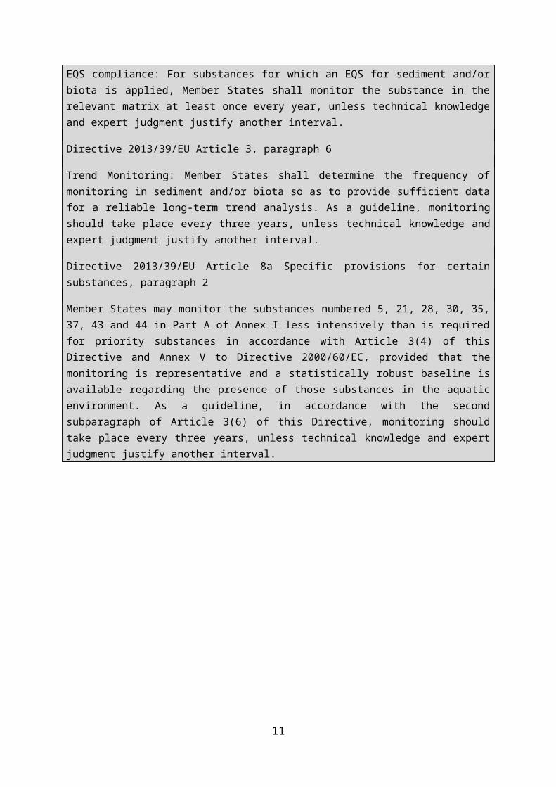
The minimum requirements of Directive 2013/39/EU for sampling frequency are:

Directive 2013/39/EU Article 3, paragraph 4

EQS compliance: For substances for which an EQS for sediment and/or biota is applied, Member States shall monitor the substance in the relevant matrix at least once every year, unless technical knowledge and expert judgment justify another interval.

Directive 2013/39/EU Article 3, paragraph 6

Trend Monitoring: Member States shall determine the frequency of monitoring in sediment and/or biota so as to provide sufficient data for a reliable long-term trend analysis. As a guideline, monitoring should take place every three years, unless technical knowledge and expert judgment justify another interval.

Directive 2013/39/EU Article 8a Specific provisions for certain substances, paragraph 2

Member States may monitor the substances numbered 5, 21, 28, 30, 35, 37, 43 and 44 in Part A of Annex I less intensively than is required for priority substances in accordance with Article 3(4) of this Directive and Annex V to Directive 2000/60/EC, provided that the monitoring is representative and a statistically robust baseline is available regarding the presence of those substances in the aquatic environment. As a guideline, in accordance with the second subparagraph of Article 3(6) of this Directive, monitoring should take place every three years, unless technical knowledge and expert judgment justify another interval.1 A ‘sample’ might comprise individual fish, or pooled fish to make up a sample large enough to provide sufficient material for analysis. For the purposes of this guidance, a sample is the material used to yield a single, measured, chemical concentration.2 This is complicated by the movement of biota, sometimes over large areas. For this reason, sampling of migratory species is discouraged.

8

2.2 Species to be sampledA key principle of this guidance is that there is no specific recommendation about which species should be sampled. The design of biota monitoring programmes should be driven by chemical risk assessment objectives, and not be limited to sites where sufficient fish populations occur. Where few/no fish occur at a desired sampling location, an alternative monitoring matrix should be employed. Consequently, flexibility in target species is required since the only species that can be sampled are those actually present at a required sampling location. It is, however, essential to be able to sample the same species (or group of species) over a period of many years (at each location). Samples must also be representative of the population and be able to be obtained annually without negative impacts on local populations.

This flexible approach to species selection also allows existing biota monitoring programmes, such as those currently utilising eels, to be accommodated within the restrictions of Guidance Document 25 (EC 2010) (i.e. “Because of their protected status, eels should only be used for existing trend monitoring (to continue existing monitoring programmes) and for this species the principle of conservation has to be respected.” (European Parliament and Council 2010)).

A wide variety of freshwater fish species from across Europe have been shown to have the capacity to accumulate pollutants (e.g. Dušek et al. 2005; Erdogrul et al. 2005; Hajšlová et al. 2007; Pulkrabova et al. 2007). There are, however, significant variations in the fish body burdens of individual substances, and these are mainly associated with the feeding and habitat preferences of different species, as well as with the fate (depuration or transformation) of the chemicals of interest (e.g. Stapleton and Baker 2003; Dušek et al. 2005; Pulkrabova et al. 2007; Sharma et al. 2009). Consequently, different temporal trends for the same substance may be observed in different species from the same locations (Bhavsar et al. 2010; Brázová et al. 2012). It may therefore be desirable to sample multiple species from different trophic levels and/or habitat types, at a single location (Burger et al., 2001).

Due to the variation in chemical residues that will result from taking biota of different species and trophic levels, steps may need to be taken to constrain as much of that variability as possible (Section 5.2.1), and to make corrections to the measured chemical concentrations to account for the major influences on bioaccumulation (i.e. lipid content, dry weight content and trophic status). This is an essential corollary to the flexibility in choice of species. Guidance on adjusting measured chemical residue data is provided in Section 6 and Annex A.8.

10

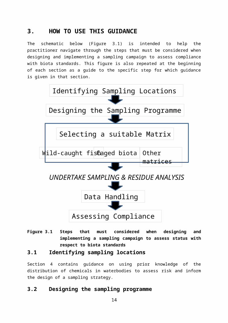
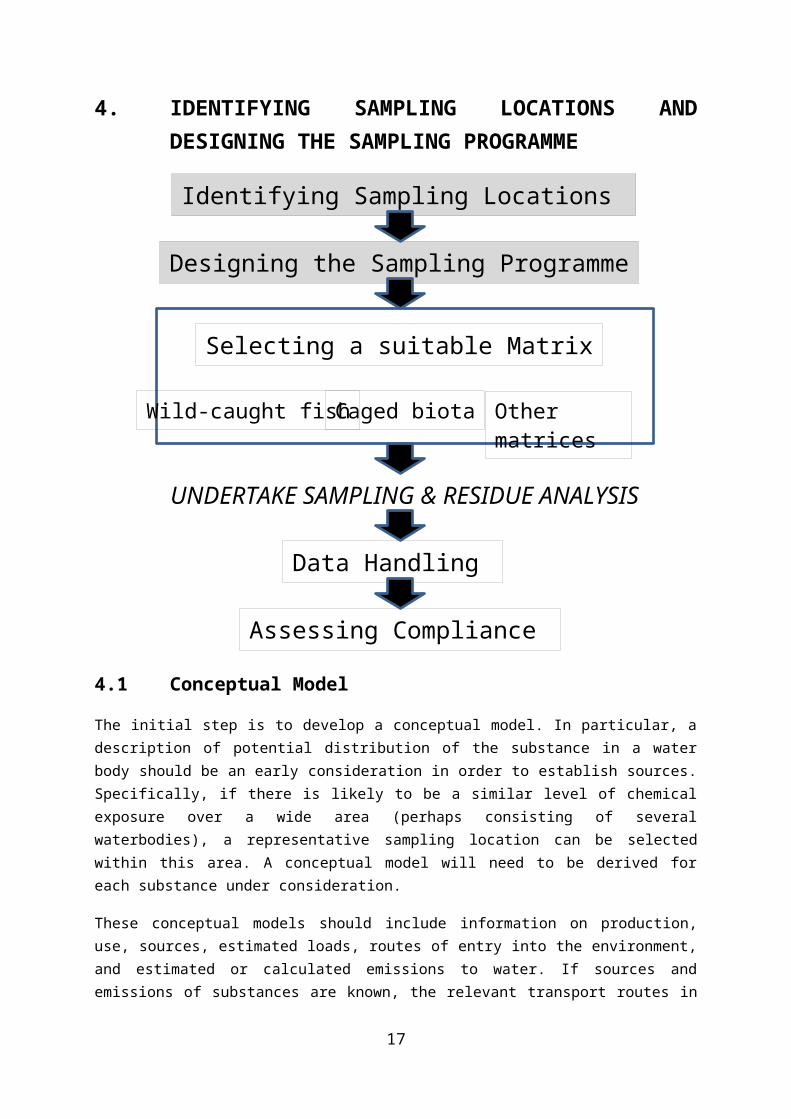
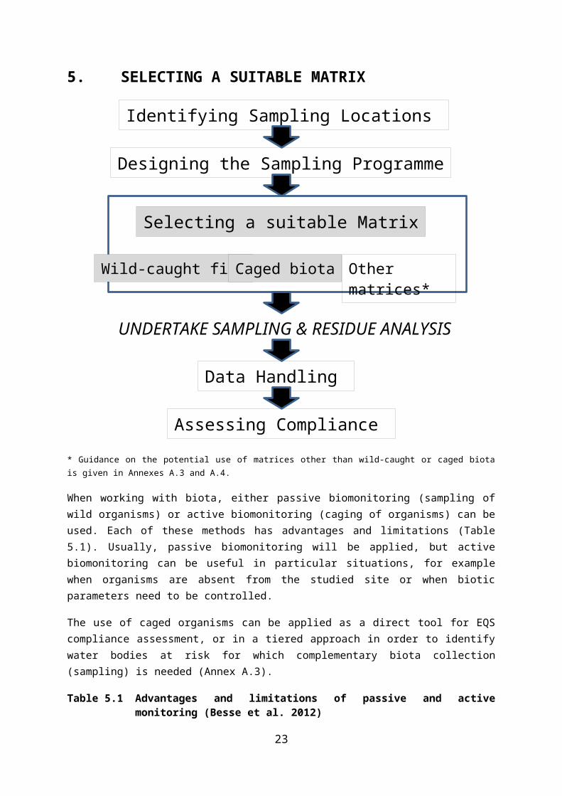
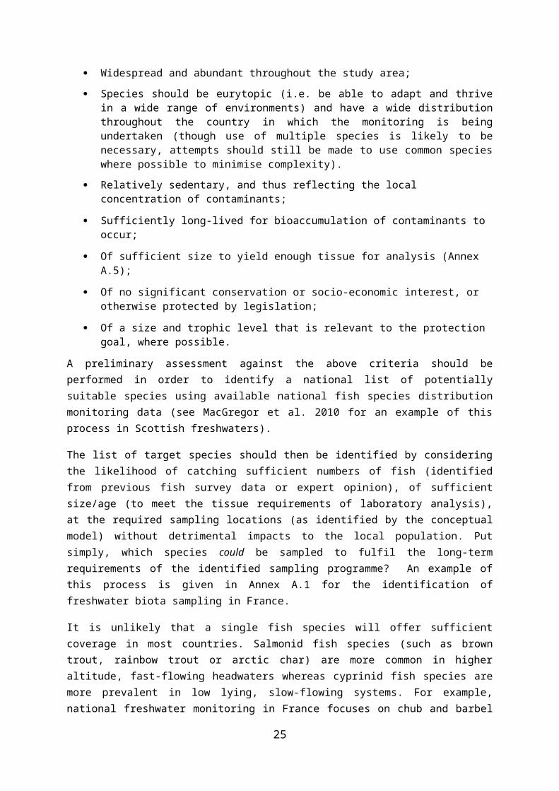
3. HOW TO USE THIS GUIDANCEThe schematic below (Figure 3.1) is intended to help the practitioner navigate through the steps that must be considered when designing and implementing a sampling campaign to assess compliance with biota standards. This figure is also repeated at the beginning of each section as a guide to the specific step for which guidance is given in that section.

Figure 3.1 Steps that must considered when designing and implementing a sampling campaign to assess status with respect to biota standards

3.1 Identifying sampling locationsSection 4 contains guidance on using prior knowledge of the distribution of chemicals in waterbodies to assess risk and inform the design of a sampling strategy.

3.2 Designing the sampling programmeSection 4.2 contains guidance on the design of a sampling approach.

11

Designing the Sampling Programme

UNDERTAKE SAMPLING & RESIDUE ANALYSIS

Assessing Compliance

Data Handling

Other matricesCaged biotaWild-caught fish

Selecting a suitable Matrix

Identifying Sampling Locations

3.3 Selecting a suitable matrixSection 5 contains guidance on the selection of the most appropriate sampling matrix based on the previous two steps.

3.4 Data handlingSection 6 contains guidance on how to relate measured chemical concentrations to the EQS.

3.5 Assessing ComplianceSection 7 explains how to use the monitoring data to assess compliance with the biota EQS, leading to a decision about chemical status.

12

4. IDENTIFYING SAMPLING LOCATIONS AND DESIGNING THE SAMPLING PROGRAMME

4.1 Conceptual ModelThe initial step is to develop a conceptual model. In particular, a description of potential distribution of the substance in a water body should be an early consideration in order to establish sources. Specifically, if there is likely to be a similar level of chemical exposure over a wide area (perhaps consisting of several waterbodies), a representative sampling location can be selected within this area. A conceptual model will need to be derived for each substance under consideration.

These conceptual models should include information on production, use, sources, estimated loads, routes of entry into the environment, and estimated or calculated emissions to water. If sources and emissions of substances are known, the relevant transport routes in a catchment area, including transport to the sea, should also be accounted for (as well as atmospheric deposition). This should be described in a quantitative and/or qualitative manner. One or more representative sampling locations should be selected for each area of homogenous chemical pressure. This might assist in reducing the sampling

13




Data Handling




burden for regional water authorities (i.e. those responsible for smaller water bodies).There may be matrices for which the currently achievable Limit of Quantification (LOQ) of the analytical methodology is not yet low enough to check compliance with the EQS. This should be indicated in the tabulated information. The uncertainties of the strategy should also be categorized and quantified, where they are known or can be resolved.

Optimisation of all the information outlined above would ideally lead to one comprehensive monitoring programme, but it might also lead to several area-specific versions. The relative costs will be an important factor influencing this decision. Another relevant aspect is whether other compounds can easily be added to the programme at a later date.

4.2 Design of a sampling programmeNotwithstanding the need for the development of a conceptual model to assist in the selection of sampling locations and the design of the monitoring programme, general guidance on the temporal and spatial elements of sampling for the assessment of compliance with EQS is well developed, and is detailed in other WFD guidance documents.

A surface water monitoring network should be established in accordance with the requirements of Article 8 of the Water Framework Directive (WFD). The monitoring network should be designed so as to provide a coherent and comprehensive overview of chemical status within each river basin.

On the basis of the characterisation and impact assessment carried out in accordance with Article 5 and Annex II of the WFD, Member States should establish, for each river basin management plan period, three types of monitoring programmes:

Surveillance monitoring programme,

Operational monitoring programme, and if necessary;

An Investigative monitoring programme.

14

Look in:Water Framework Directive 2000/60/EC Article 8 and Annex V (EC 2000)Member States shall ensure the establishment of programmes for the monitoring of water status in order to establish a coherent and comprehensive overview of water status within each river basin district.

Water Framework Directive 2000/60/EC Annex V 1.3.1 Guidance Document No. 7 - Monitoring Under the Water

Framework Directive, 2.7.2 Guidance Document No. 19 – Guidance on Surface Water

Chemical Monitoring under WFD, 4.5.

Biota monitoring may be undertaken for each of these types of monitoring, with the greatest experience in Europe associated with surveillance monitoring. Investigative monitoring is discussed further in Annex A.3.

Operational monitoring, for compliance assessment, shall be undertaken in order to establish the status of those bodies identified as being at risk of failing to meet their environmental objectives, and assess any changes in the status of such bodies resulting from the programmes of measures. Operational monitoring is characterised by spatially and temporally flexible monitoring networks, problem-oriented parameter selection and sampling.

Monitoring of biota to assess compliance with biota standards should be undertaken at least once per year at each sampling location.

A practical criterion that should be considered is the opportunity to combine biota monitoring programmes for EQS compliance and biota sampling for ecological assessment, especially fish sampling. This makes it possible to obtain biota samples without further budget investments as well as enabling a full biological characterization of the biota samples that are subject to chemical assessment.

4.2.1 How many samples are needed?

The number of samples required for the assessment of compliance with an EQSbiota is informed by:

● The expected (or measured) variability in chemical residues between samples, and;

● Decisions about the required level of confidence in compliance assessments.

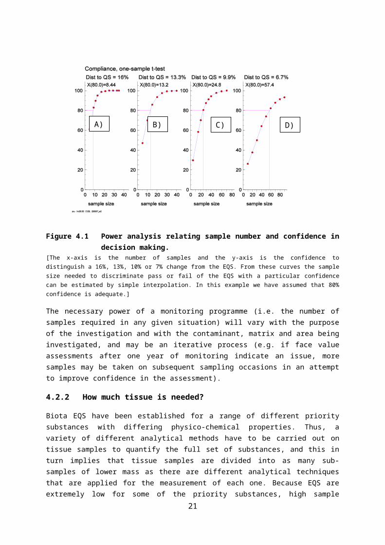
The relationship between variability, sample size and confidence in the decisions made based on sampling can be illustrated using a power curve (Figure 4.1). Where high confidence of failure of the EQS is required, increased numbers of failed sites are delivered by increased sampling. In other words, smaller degrees of exceedance are detected with high confidence. In the example below, for each sample size (dots) 1000 randomized sample trials were carried out and the proportion showing compliance were recorded. The sample size that resulted in

15

Look in: Water Framework Directive 2000/60/EC Annex V 1.3.2 Guidance Document No. 7 - Monitoring Under the Water

Framework Directive, 2.8.2 Guidance Document No. 19 – Guidance on Surface Water

Chemical Monitoring under WFD, 4.6 Guidance Document No. 25 – Guidance on chemical

monitoring of sediment and biota under WFD (2010), 6.2.3.

success in 80% of all trials was estimated through interpolation. The various plots (A-D from left to right) represents decreasing distances to the Quality Standard (QS). The closer the true data are to the QS, the larger the required sample size needs to be in order to tell whether the EQS has been exceeded or not.

If there are no existing data about variability between samples, it may be necessary to instigate a small pilot study to estimate it. These data can then be used to construct a power curve like the one shown in Figure 4.1 from which the number of replicates required can be estimated. Alternatively, it may be possible to use data obtained from studies of similar species in other regions.

If it is expected that levels of chemical contamination are markedly different from the EQS (either much lower, or much higher), then fewer samples can discern, with confidence, the difference between residues in biota and the EQSbiota.

Figure 4.1 Power analysis relating sample number and confidence in decision making.

[The x-axis is the number of samples and the y-axis is the confidence to distinguish a 16%, 13%, 10% or 7% change from the EQS. From these curves the sample size needed to discriminate pass or fail of the EQS with a particular confidence can be estimated by simple interpolation. In this example we have assumed that 80% confidence is adequate.]

The necessary power of a monitoring programme (i.e. the number of samples required in any given situation) will vary with the purpose of the investigation and with the contaminant, matrix and area being investigated, and may be an iterative process (e.g. if face value assessments after one year of monitoring indicate an issue, more samples may be taken on subsequent sampling occasions in an attempt to improve confidence in the assessment).

4.2.2 How much tissue is needed?16

D)C)B)A)

Biota EQS have been established for a range of different priority substances with differing physico-chemical properties. Thus, a variety of different analytical methods have to be carried out on tissue samples to quantify the full set of substances, and this in turn implies that tissue samples are divided into as many sub-samples of lower mass as there are different analytical techniques that are applied for the measurement of each one. Because EQS are extremely low for some of the priority substances, high sample volumes will be needed to meet the minimum performance criteria for chemical analysis, laid down by EC directive 2009/90. The tissue weight requirement for individual analysis will further depend on the species and size/ age of individuals selected, the available sampling equipment, the method to be applied for chemical analysis, the concentration of contaminant in the sample and the lipid content (for lipophilic contaminants).

Detailed guidance on tissue weight requirements are given in Annex A.5. This reflects the current practice in effect within ongoing national programmes for the monitoring of contaminants in biota.

Overall, more than 100g wet weight of material (fish or bivalves) is required to analyse trace metals, PAHs and other organic contaminants.

17

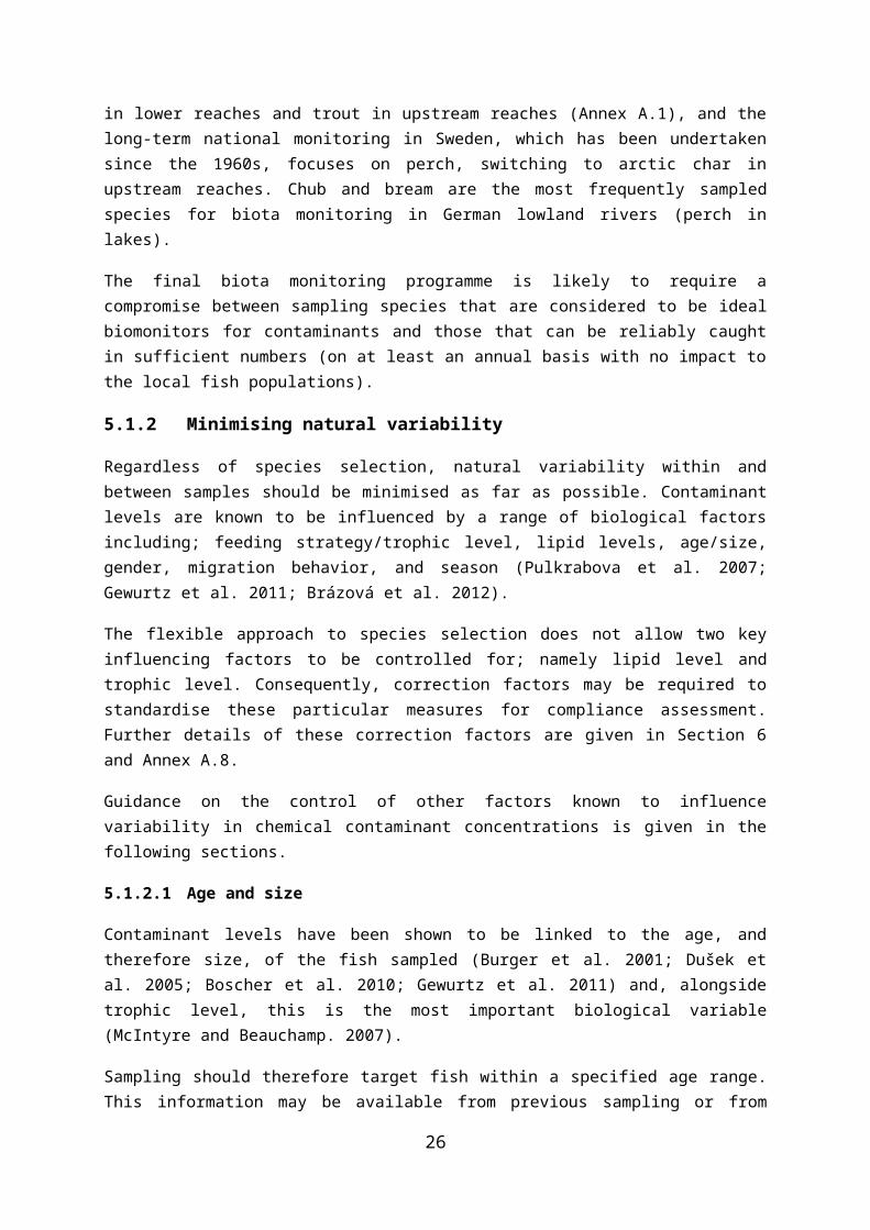
5. SELECTING A SUITABLE MATRIX

* Guidance on the potential use of matrices other than wild-caught or caged biota is given in Annexes A.3 and A.4.

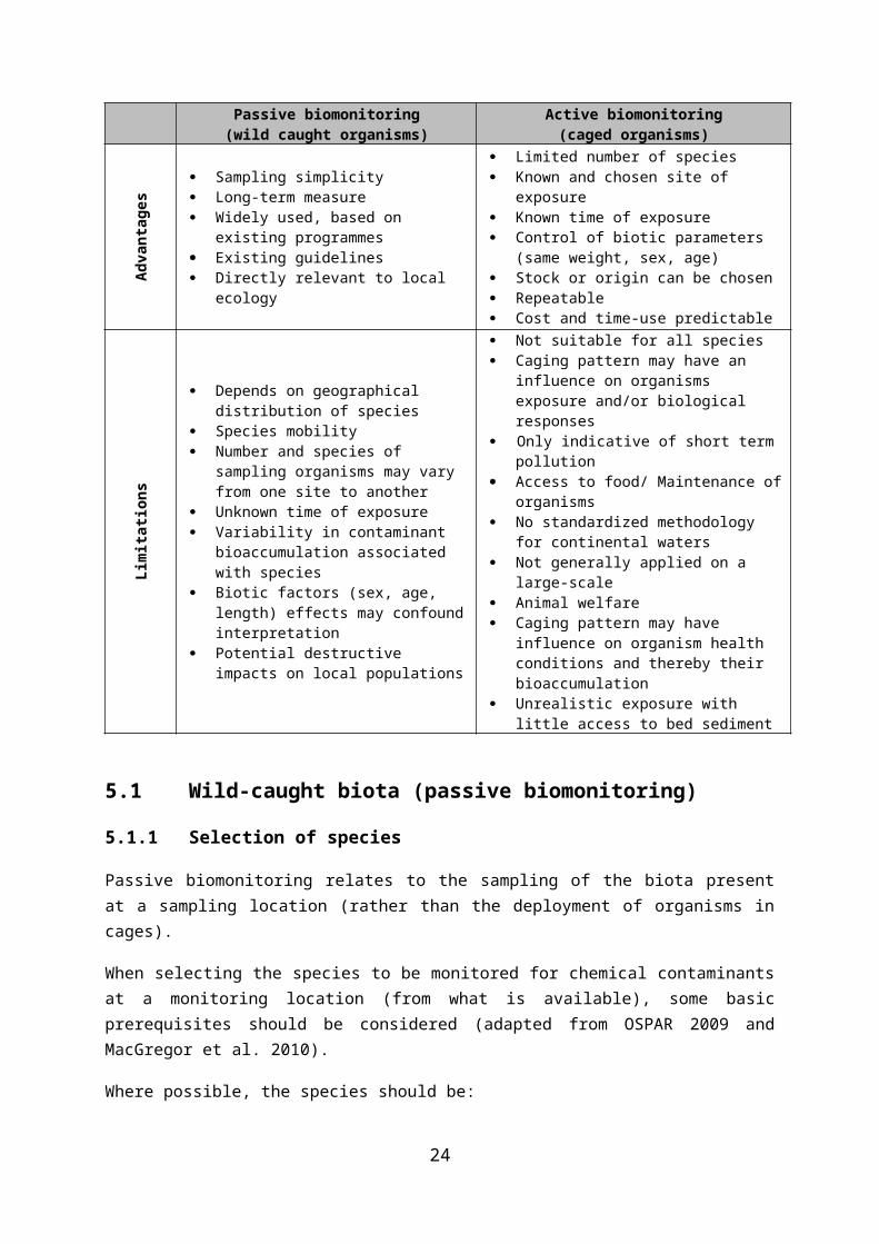
When working with biota, either passive biomonitoring (sampling of wild organisms) or active biomonitoring (caging of organisms) can be used. Each of these methods has advantages and limitations (Table 5.1). Usually, passive biomonitoring will be applied, but active biomonitoring can be useful in particular situations, for example when organisms are absent from the studied site or when biotic parameters need to be controlled.

The use of caged organisms can be applied as a direct tool for EQS compliance assessment, or in a tiered approach in order to identify water bodies at risk for which complementary biota collection (sampling) is needed (Annex A.3).

Table 5.1 Advantages and limitations of passive and active monitoring (Besse et al. 2012)

Passive biomonitoring(wild caught organisms)

Active biomonitoring(caged organisms)

18




Data Handling

Other matrices*Caged biotaWild-caught fish



Adva

ntag

es Sampling simplicity Long-term measure Widely used, based on existing

programmes Existing guidelines Directly relevant to local ecology

Limited number of species Known and chosen site of exposure Known time of exposure Control of biotic parameters (same

weight, sex, age) Stock or origin can be chosen Repeatable Cost and time-use predictable

Lim

itat

ions

Depends on geographical distribution of species

Species mobility Number and species of sampling

organisms may vary from one site to another

Unknown time of exposure Variability in contaminant

bioaccumulation associated with species

Biotic factors (sex, age, length) effects may confound interpretation

Potential destructive impacts on local populations

Not suitable for all species Caging pattern may have an

influence on organisms exposure and/or biological responses

Only indicative of short term pollution

Access to food/ Maintenance of organisms

No standardized methodology for continental waters

Not generally applied on a large-scale

Animal welfare Caging pattern may have influence

on organism health conditions and thereby their bioaccumulation

Unrealistic exposure with little access to bed sediment

5.1 Wild-caught biota (passive biomonitoring)

5.1.1 Selection of species

Passive biomonitoring relates to the sampling of the biota present at a sampling location (rather than the deployment of organisms in cages).

When selecting the species to be monitored for chemical contaminants at a monitoring location (from what is available), some basic prerequisites should be considered (adapted from OSPAR 2009 and MacGregor et al. 2010).

Where possible, the species should be:

Widespread and abundant throughout the study area; Species should be eurytopic (i.e. be able to adapt and thrive in a wide

range of environments) and have a wide distribution throughout the country in which the monitoring is being undertaken (though use of multiple species is likely to be necessary, attempts should still be made to use common species where possible to minimise complexity).

Relatively sedentary, and thus reflecting the local concentration of contaminants;

Sufficiently long-lived for bioaccumulation of contaminants to occur;

19

Of sufficient size to yield enough tissue for analysis (Annex A.5); Of no significant conservation or socio-economic interest, or otherwise

protected by legislation; Of a size and trophic level that is relevant to the protection goal, where

possible.A preliminary assessment against the above criteria should be performed in order to identify a national list of potentially suitable species using available national fish species distribution monitoring data (see MacGregor et al. 2010 for an example of this process in Scottish freshwaters).

The list of target species should then be identified by considering the likelihood of catching sufficient numbers of fish (identified from previous fish survey data or expert opinion), of sufficient size/age (to meet the tissue requirements of laboratory analysis), at the required sampling locations (as identified by the conceptual model) without detrimental impacts to the local population. Put simply, which species could be sampled to fulfil the long-term requirements of the identified sampling programme? An example of this process is given in Annex A.1 for the identification of freshwater biota sampling in France.

It is unlikely that a single fish species will offer sufficient coverage in most countries. Salmonid fish species (such as brown trout, rainbow trout or arctic char) are more common in higher altitude, fast-flowing headwaters whereas cyprinid fish species are more prevalent in low lying, slow-flowing systems. For example, national freshwater monitoring in France focuses on chub and barbel in lower reaches and trout in upstream reaches (Annex A.1), and the long-term national monitoring in Sweden, which has been undertaken since the 1960s, focuses on perch, switching to arctic char in upstream reaches. Chub and bream are the most frequently sampled species for biota monitoring in German lowland rivers (perch in lakes).

The final biota monitoring programme is likely to require a compromise between sampling species that are considered to be ideal biomonitors for contaminants and those that can be reliably caught in sufficient numbers (on at least an annual basis with no impact to the local fish populations).

5.1.2 Minimising natural variability

Regardless of species selection, natural variability within and between samples should be minimised as far as possible. Contaminant levels are known to be influenced by a range of biological factors including; feeding strategy/trophic level, lipid levels, age/size, gender, migration behavior, and season (Pulkrabova et al. 2007; Gewurtz et al. 2011; Brázová et al. 2012).

The flexible approach to species selection does not allow two key influencing factors to be controlled for; namely lipid level and trophic level. Consequently, correction factors may be required to standardise these particular measures for compliance assessment. Further details of these correction factors are given in Section 6 and Annex A.8.

20

Guidance on the control of other factors known to influence variability in chemical contaminant concentrations is given in the following sections.

5.1.2.1 Age and size

Contaminant levels have been shown to be linked to the age, and therefore size, of the fish sampled (Burger et al. 2001; Dušek et al. 2005; Boscher et al. 2010; Gewurtz et al. 2011) and, alongside trophic level, this is the most important biological variable (McIntyre and Beauchamp. 2007).

Sampling should therefore target fish within a specified age range. This information may be available from previous sampling or from local fisheries staff. Best practice would be to verify the age of the fish in the laboratory using otolithes or scales.

In the UK, published literature (Britton, 2007) has been used to develop a look-up table that relates age to size for a range of freshwater fish species. This relationship will vary in other countries in response to temperature and productivity, but may act as a guide in the absence of better information3.

The length of the individuals of each species collected should be constant from year to year at each sampling location, or should at least fall within a consistent range. A pragmatic choice of fish age is between 3-5 years, but practical considerations in the field and laboratory (e.g. tissue volume requirements) may override this (Annex A.5).

5.1.2.2 Migration behaviour

Many species undertake seasonal migration during their life cycle (e.g. for reproduction, foraging or overwintering), and for some species individuals may cover tens to hundreds of kilometres. Hence, to be able to report on the local pollution pressure it is essential to choose a relatively sedentary, non-migratory species. In most species, migration behaviour is relatively well studied, and may be deduced from scientific literature.

In sedentary species, individuals taken at one site should show similar levels/profiles of contamination (e.g. Belpaire et al. 2008). Sampling should therefore be directed at sedentary species most likely to be representative of the sampling location.

However, for the purposes of MSFD, less sedentary species can be relevant since the areas to assess under MSFD are generally larger than water bodies under WFD.

5.1.2.3 Condition factor

3 E.g. http://www.fishbase.org/search.php21

http://www.fishbase.org/search.php

The condition factor (K)4 of fish has been associated with the contaminant levels in some studies (e.g. Farkas et al. 2003) but has shown weaker/no correlation in others (e.g. Noel et al. 2013). The relationship between contaminant load and condition factor may be substance specific. For example, Noel et al. (2013) observed no correlation between condition factor and the trace elements arsenic, cadmium and lead, but a positive correlation with mercury levels.

As variation in condition factor may be closely associated with the seasonality of sampling (Farkas et al. 2003), the K value is unlikely to be a large contributor to variation except where fish are in extremely poor condition, providing that appropriate control measures are employed (Section 5.1.2.5).

Fish measurement data (length and weight) collected during field sampling should allow condition factor to be determined and taken into account if necessary (e.g. widely varying measurements).

5.1.2.4 Gender

Contaminant loads may differ between the different sexes of fish (Sharma et al. 2009). Possible explanations for these differences are; the potential elimination of lipophilic pollutants by females in roe at spawning (Sharma et al. 2009), differences in habitat utilization leading to sex differences in substance concentrations of prey, or sex differences in gross growth efficiency (Madenjian et al. 2011).

Different mechanisms may operate in different species for influencing the degree of variation between sexes (Madenjian et al. 2011). This is supported by the results of Sharma et al. (2009), who found differences between sexes in pike, but not perch.

Directing sampling of a particular sex would obviously control for any potential gender differences, and some biota monitoring guidance (e.g. JAMP guidance for the marine environment) suggests sampling all female fish. However, this could potentially result in an underestimation of contaminants should contaminant levels be reduced by spawning. Conversely, sampling all males may overestimate contamination if higher metabolic demands of males lead to increased food consumption (Madenjian et al. 2011).

Considering that sex cannot be differentiated in most species prior to sampling, no recommendation is made on standardising for gender. Best practise would be to determine the sex of individuals analysed and use the data gathered to inform future guidance.

4 Condition factor (K) employs the relationship between the weight of a fish and its length, to provide a descriptor of the “condition” of that individual (Nash et al., 2006) and is calculated by the formula:

K=100 (W/L3)where W is the whole body wet weight in grams and L is the length in centimetres; the factor 100 is used to bring K close to a value of one.

22

5.1.2.5 Seasonality

Chemical residues accumulated by biota can be affected by season, particularly when fish are approaching the breeding season. In cases where females are used, contaminant levels may have dropped during reproduction through maternal transfer into the eggs. Significantly lower levels of PBDE and PCBs have been measured in roach and perch in July after spawning compared with earlier in the year (Noel et al. 2013). Considerable seasonal variations in contaminants have also been reported in bream (Farkas et al. 2003).

Sampling during and immediately before/after the breeding period should therefore be avoided, and sample timing at a location should be consistent from year to year.

For practical reasons, Member States may decide to combine sampling efforts for analysis of contaminants in biota with the sampling procedures and field actions associated with fish stock assessments for evaluating ecological quality. In this case, the most optimal period of sampling should be chosen to find the acceptable compromise between the objectives of both types of monitoring.

23

5.1.2.6 Stocked versus indigenous populations

Stocked fish may have been present in the waterbody for only a short period and therefore may underestimate the exposure period, and therefore accumulation, experienced by indigenous populations. Moreover, they may have been subject to contaminant pressure during holding at the fish culture unit, so may already have significant contaminant levels when they are stocked.

Ideally, areas with known stocking activity should be avoided and stocked fish (if they can be identified) should not be sampled. If this is not possible, sampling should take place after a sufficiently long period has elapsed following stocking for their contaminant levels to reflect the local situation (similar to caged biota).

24

5.2 Caged biota (active biomonitoring)As indicated above, passive biomonitoring (i.e. the sampling of the biota present at a sampling location) may not be possible if suitable organisms are not present at the selected monitoring sites (Table 5.1) (Besse et al. 2012; 2013). In such circumstances, active biomonitoring (i.e. the introduction of caged organisms) can be a viable alternative.

5.2.1 Species selection

There are two main possibilities in selecting a group of organisms for caging:

Fish are an appropriate organism for checking compliance against biota EQS. However their use is not recommended for active biomonitoring. Caging is usually unsuitable for fish because their size requires large caging systems that are difficult to handle, and the fish are easily stressed, particularly in caging systems which limit their mobility (Besse et al. 2012).

Invertebrates represent a good compromise in terms of feasibility and fulfilling the objectives of the WFD, since they also represent a food source for secondary predators and humans, and their smaller size facilitates handling and caging. The use of invasive species should be avoided (e.g. the zebra mussels Dreissena polymorpha and the Asian clam Corbicula fluminea). However, the use of these species can be tolerated if they are only used at sites that they have already colonized (Besse et al. 2012).

5.2.2 Minimising variability

Several considerations need to be made when using caged organisms.

Similar weight or similar size organisms should always be selected for caging. In the case of molluscs, some researchers consider weight as the primary factor that can influence levels of contaminants (Andral et al. 2004; Conti et al. 2008). These variations may stem from several sources: growth rate of juvenile individuals, reproductive cycle (see below), and food availability. The size of the organisms should be measured before and after caging in order to calculate the growth rate which constitutes an important parameter for the calculation of the contaminant uptake. If the exposure duration is long enough to lead to a modification of the size and/or weight of the organisms during the caging period, it is recommended that the contamination levels are normalised against the condition factor (5.1.2.3).

As stated above (5.1.2.5) the breeding period of species can affect the accumulation of contaminants. This reproductive cycle-related issue should be controlled in one of two ways. If the organisms do not present any differentiable sexual dimorphism, as is the case in most bivalve molluscs, then caging has to be scheduled outside the reproductive periods, during which metabolism remains stable. If the sexes can be differentiated (e.g. freshwater amphipods), then it is

25

recommended to use same-sex individuals, males will usually be preferred, at a well-defined reproductive stage.

The mortality level during the experiment should also be taken into account (Besse et al., 2013; Gust et al. 2010; 2011; Turja et al. 2013). An acceptable mortality level of 10 to 20% in the reference site is generally considered to be acceptable.

In order to obtain comparable results, it is important to use organisms belonging to an identical population. Reference sites can be a reliable source of organisms, but must be unpolluted with good water quality. Laboratory cultures of organisms may also be used (e.g. Gust et al. 2010; 2011; Bervoets et al. 2009). Analysis of individuals from the population to be caged for the substances of interest should be undertaken to ensure that the organisms are not contaminated prior to deployment.

Conditioning in the laboratory before deployment is recommended to allow organisms to recover from the sampling process and possible oxygen deficiency during transport. Organisms should also be cleaned and rinsed with water directly after sampling to remove sand, silt and other impurities that may be contaminated with the substances of interest.

During depuration, parameters such as temperature, oxygen, and light cycle should be controlled to meet the most appropriate possible conditions for the chosen species. Hardness, temperature, pH and other physicochemical parameters of the reference site and the subsequent studied site should also be taken into consideration.

Previously caged organisms can generally be held in the laboratory for a few days without the need for additional feeding. Acclimatisation periods longer than this should be avoided, since food may need to be provided. The addition of uncontaminated food reflects neither field nor laboratory exposure and will affect the concentration of substances accumulated during the caging period.

5.2.3 Caging systems

The parameters that should be considered when developing a caging system include the size of the cages (according to species), the mesh size, the number of organisms per cage and the number of cages per site. When caging invertebrates, cages should be constructed from rigid plastic containers with both extremities replaced by mesh (Lacaze et al. 2011; Gust et al. 2010; 2011; Turja et al. 2013). The size of the mesh will depend on the species to be caged. Organisms should obviously not be able to escape from the cage, but the size of the mesh should also be carefully chosen to limit clogging by suspended matter but to allow food particles to enter the cage. These containers can be placed side by side in larger cages when grouping several replicates.

Fish caging is not recommended. However, if used, it requires particular attention to be paid to the caging system in order to limit negative effects on fish health. It

26

is recommended to use non-abrasive surfaces (e.g. polyethylene) for each part of the cage that comes into contact with the fish. This will avoid lesions from repeated contact of the fish with the side of the cage. The use of opaque cages is recommended because this provides a visual barrier which discourages escape attempts and fish movements in response to stimuli from outside the cage, and limits contact with the cage and possible abrasion.

For all caging systems, their position should allow a good circulation of water (Hannah et al. 2012). It is therefore important to pay attention to the direction of the water flow when siting the cage (Besse et al. 2013). Cages can either be secured to the stream bed (e.g. using rocks as ballast) or be suspended in the water column with an anchor and buoy system (which will regulate their depth). The cage should be deep enough in the water to resist the movement of the current and should be isolated from movements caused by the mooring line, particularly if fish are caged (Hannah et al. 2012).

5.2.4 Duration and timing of deployment

The duration of caging will depend on the species used and the time necessary to accumulate the selected pollutants (but can be up to 6 weeks). A pre-exposure study should be undertaken to determine the appropriate caging duration for the chosen organisms and substances. The duration of caging should always allow for the organisms to equilibrate with the new environmental conditions (Marigomez et al. 2013; Herve et al. 2002; Giltrap et al. 2012).

Usually, the recommended seasons for caging would be summer and autumn, but it is important to adapt these recommendations to the chosen species. In every instance, caging should be conducted at the same period each year in order to limit the variability due to seasonal influences (e.g. breeding cycles, water temperature) and to allow comparisons between results.

27

5.3 Choice of tissue for contaminant analysisWhether wild-caught or caged organisms are used at a particular site within the overall biota monitoring programme, there should be a clear link between the EQS and the tissue that is analysed for comparison with the EQS.

For example, if an EQSbiota is designed to protect the secondary predators that consume fish, then the analysis should be related to whole fish, and not just one part of the fish (e.g. muscle meat or liver tissue).

The choice of appropriate tissue can be influenced by:

The monitoring purpose (detection of spatial and/or temporal trends or assessment of compliance with suitable effect thresholds or guideline concentrations);

The classes of investigated chemicals (lipophilic contaminants which differentially partition into fatty tissue, or contaminants with high affinity for protein-rich tissue/organ);

Tissue availability (quantity of biological material compatible with minimum performance criteria for methods of chemical analysis laid down by the commission directive 2009/90/EC).

5.3.1 Current practice from ongoing monitoring programmes

In nine biota monitoring programmes currently ongoing across Europe (Table 5.2), bivalves, crustaceans and fish are the most commonly used organisms for monitoring contaminants.

For smaller species, such as most invertebrates, the only practical option is to measure contaminants in the whole organism. Samples are often composited when individuals do not have a sufficient mass to allow for detection of the analyte. Bivalves are usually analysed individually or composited. For crustaceans, the edible parts of crustaceans (i.e. muscle meat from appendages and abdomen) are generally sampled if the main objective includes human health concerns.

For fish, one of several tissue types are typically monitored, i.e. homogenised whole fish, muscle, liver and, occasionally, kidney, and the choice between them depends on the goal of the monitoring programme and the type of EQS used for compliance assessment.

When assessing compliance using fish, contamination is usually evaluated by analysing muscle fillets relative to human health exposure or whole fish relative to wildlife exposure. Because humans most frequently consume only the fish fillet portion of the majority of fish, consumption advisory criteria are typically based on fillet contaminant concentrations, and therefore fillet data are those usually those most readily available (Table 5.2). Whole-fish data which can be used to

28

address questions regarding bioaccumulation, food-web transfer and to assess the risk toward piscivorous wildlife (birds and mammals) are frequently scant.

Depending on how fish are prepared, consumers may have significantly differing exposures to chemical contaminants. Many people remove the internal organs before cooking fish and trim off fat and skin before eating, thus decreasing exposure to lipophilic and other contaminants. Trimming has been shown to reduce total concentrations of PCBs by 40-60% in fish (Williams et al. 1992). Certain populations eat parts of the fish other than the fillet (e.g. liver) or may consume the fillet with the skin. As a result, more of the fish contaminants are consumed.

In the ongoing programmes detailed in Table 5.2, fish fillets are usually analysed without the skin. The remaining parts of the muscle meat and fat tissue on the inner side of the skin are occasionally scraped off from the skin and added to the sample to be analysed, consistent with EC 2006, which lays down methods of sampling and analysis for official control levels of dioxins and dioxin-like PCBs in certain foodstuffs. As both fat and water content vary significantly in the muscle tissue from the anterior to the caudal muscle of a fish, it is important to obtain the same proportion of the muscle tissue for each sample. Ideally, whole muscle tissue should be homogenised first and then divided into as many sub-samples as needed to cover the whole range of chemicals analysed. This also holds true for whole fish samples.

29

Table 5.2 Species/tissues used currently in European biota monitoring programmesProgramme / convention Purposes of the monitoring Contaminants

measuredBiotaTissue / organ

Protocol for the dissection and collection of tissue samples

Joint Assessment and Monitoring Programme (OSPAR)

International / regional

- Temporal trend monitoring

- Spatial distribution of pollution

- Assess possible hazards to human health and harm to living resources and marine life

- Including:- Metals (Cd, Hg, Pb)- Organic

contaminants such as parent and alkylated PAHs, PBDEs, HBCDD, PFCs, organotin compounds, PCDD/F and dioxin-like PCBs

MusselWhole soft body (pool consisting of at least 20 individuals)Pacific oysterWhole soft bodyFlatfish (dab, plaice, flounder)Muscle* for Hg and liver for all other contaminants (fish analysed individually)Roundfish (cod, whiting, hake, herring)Muscle for Hg and liver for all other contaminants

*When sampling fish muscle, care should be taken to avoid including any epidermis or subcutaneous fatty tissue in the sample.

JAMP guidelines for monitoring contaminants in biota, OSPAR Commission, agreement 1999-02, revised 2012

Combine programme of HELCOM


- Compare the level, of contaminants in biota from different geographical regions

- Measure levels of contaminants in biota over time at specific locations

- Measure levels of contaminants in selected biota species to assess possible harm to these species or to higher trophic levels (comparison with BAC or EAC from OSPAR or EU foodstuff limits)

- Metals (Cd, Hg, Pb)- PAHs- PCDD/Fs and dioxin-

like PCBs- PCBs- Organochlorine

pesticides (DDTs and DDE, HCH, HCB)

- BFRs (PBDEs, HBCDD)- PFCs- TBT

Blue musselWhole soft bodyFish (herring, plaice, cod, eelpout)Muscle tissue / liver depending on the contaminants to be analysed

Manual for marine monitoring in the COMBINE programme of HELCOM (updated in 2013)

30

Programme / convention Purposes of the monitoring Contaminants measured

BiotaTissue / organ


MEDPOL


- Spatial and temporal trend monitoring

- Compliance assessment monitoring

- Metals (Cd, Hg, Pb, Cu, Zn)

- PCBs- Organochlorine

pesticides (DDTs, aldrin, endrine, dieldrin, HCB and lindane)

Mollusc bivalvesWhole soft tissueDemersal fishMuscle (selected for public health concerns) / liver, kidney and other tissues or target organs of specific contaminantsCrustaceansHepatopancreas / whole edible tissue if main objective includes human health concerns

UNEP/FAO/IAEA reference methods for marine pollution studies

Convention on the Protection of the Rhine


Compendium of information from national monitoring programmes(GER, FR, NL, LUX, CH)

- PCDD/Fs and dioxin-like PCBs

- PCBs- HCB- Hg

Fish (Eel, roach, bream, chub)Muscle (fillet*) and occasionally liver and kidney

*Skinless fish fillet as the maximum level applies to muscle meat without skin. However it is necessary that all remaining rests of the muscle meat and fat tissue at the inner side of the skin are carefully and completely scraped off from the skin and added to the sample to be analyses.

Reference to the commission regulation No 1883/2006 laying down methods of sampling and analysis for the official control levels of dioxins and dioxin-like PCBs in certain foodstuffs

Joint commission for the protection of Italian-Swiss waters against pollution (CIPAIS)


- Temporal trend monitoring

- Spatial distribution of pollution

- Assess risk toward human health and ecosystem

- Metals (As, Cd, Hg, Pb, Ni, Cr)

- Organic contaminants (PAHs, PBDEs, PCBs, Organochlorines)

Benthic invertebratesWhole bodyMussel (Dreissena polymorpha)Whole soft bodyFish (Roach, whitefish, landlocked shad)Muscle (caudal fillet)

www.cipais.orgAnnual reports

Swedish contaminant monitoring programme in marine and freshwater biota

National

The monitoring programme has many objectives among which:- Estimates the current

levels of various contaminants in aquatic biota from several representative sites

- Metals (Hg, Pb, Cd, Ni, Cr, Cu, Zn, As, Ag)

- PCBs- DDTs- HCHs- HCB- PCDD/Fs- BFRs( PBDEs,

Marine watersBlue musselWhole soft tissue (metals are analysed in individual mussels and samples for organochlorine, bromine determination and PAHs are analysed in pools of 20 specimens)Fish (herring, cod, eelpout, dab, flounder)Muscle tissue* for BFRs, organochlorine compounds and Hg / liver for metals and PFAAs analyses

Report from the Swedish Museum of Natural History“Comments concerning the national Swedish contaminants monitoring programme in marine biota”

31

http://www.cipais.org/

Programme / convention Purposes of the monitoring Contaminants measured

BiotaTissue / organ


influenced by local sources- Monitor long term time

trends- Indicate large scale spatial

differences- Determine whether the

quality of fish is suitable for human consumption (comparison with target levels)

HBCDD)- PAHs- PFCs

*Muscle samples are taken from the middle dorsal layer. The epidermis and subcutaneous fatty tissue are carefully removed.

FreshwatersFish (pike, arctic char, perch, roach - formerly)Muscle tissue analysed individually or as a pool sample for organochlorines, BFRs, PAHs and Hg / liver for metals and PFAAs.

and

TemaNord 1995:543. Manual for Nordic Environmental Specimen Banking

German environmental specimen programme

National

Monitor the changes in the concentration of various pollutants over the course of time

Various pollutants Zebra musselWhole soft bodyBream

Muscle tissue* and liver

*Skinless fish fillet obtained by the incision of the muscle tissue along the dorsal line and along the upper edge of the spine and its removal from head to tail.

Standard operating procedures for all the relevant steps (sampling, sample preparation, conservation, storage, and analysis) are available on the ESB website

WFD Monitoring of the Federal States of Germany

National

Trend monitoring; Compliance monitoring

Hg, HCB, HCBD and others

RiversFish (Chub, bream, roach, perch, trout, eel)LakesFish (Perch bream, roach, pike, whitefish, char)Muscle tissue without the skin (Individual or pool samples)

RAKON B, Part IV.3 and IV.1 (Framework concept for monitoring of the LAWA, the German working group on water issues of the Federal States and the Federal Government)

UK fish tissue archive

National

Various pollutants Roach, and occasionally bleak and eelWhole fish / liver and gall bladder are also sampled in some specimens

32

5.3.2 Implications of using whole fish versus fish tissues/ organs when assessing compliance

Chemical contaminants are not distributed uniformly in fish. Fatty tissues, for example, will concentrate hydrophobic organic chemicals more readily than muscle tissue. Muscle tissue and viscera will preferentially concentrate other contaminants. This has important implications for fish analysis and fish consumers. Depending on which parts are eaten, consumers may have significantly differing exposures to chemical contaminants.

The lipid content of the different tissues is important when considering the distribution of substances. If none, or a minor part, of the substance is bio-transformed into hydrophilic metabolites, the tissue distribution of the substance would be expected to reflect the lipid content of the different tissues, given that the time has been sufficient for inter-organ steady state concentration to be achieved (Gobas et al. 1999). Lipophilic chemicals accumulate mainly in fatty tissues, including the belly flap, lateral line, subcutaneous and dorsal fat, and the dark muscle, gills, eyes, brain, and internal organs. Muscle tissue often contains lower organic contaminant concentrations than fatty tissues but contains more mercury, which binds to muscle proteins. Contaminants with high affinity for protein-rich tissue/organ, such as PFOS, concentrate more in the liver and kidney (Goeritz et al. 2013; Martin et al. 2003).

In most cases, it would be advantageous to have both the whole fish and the fillet data for the same individual, but, unfortunately, budget constraints generally dictate that samples are only analysed in one or the other sample type. Fillet concentrations may not accurately represent, or predict, concentrations in the whole body because of chemical-specific differences in assimilation rates and affinities for various tissue compartments and organs.

Thus, it is usually assumed that fillet concentrations are some fraction of the whole fish concentration for lipophilic compounds when expressed on a wet weight basis (Uhl et al. 2010), due to the presence of fatty internal organs that are included in whole fish measurements (i.e. fillet concentrations will be lower than comparable whole fish concentrations, since whole fish tend to have a greater percentage of lipids). Differences do, however, exist between fish species. Fish with higher lipid contents generally store more lipids in the fillet portion than lean fish, which store most of their lipids in the viscera and head, which are not included in the edible portion.

As a consequence, use of fillet data may underestimate the risks to piscivorous wildlife and to people who consume whole fish. Conversely, whole-body contaminant concentrations in fish would overestimate the risk associated with consuming only fillet portion of the fish, with the exception of mercury which is generally underestimated.

Directive 2013/39/EC (EC 2013) sets biota EQS for 11 priority substances. Human health is the protection goal for seven priority substances; top predators are identified as receptors at risk for the remaining four priority substances (Table

33

5.3). For some chemicals, the quality standards derived for the two receptors (QSbiota,hh and QSbiota,secpois) are very similar (ratios close to 1) and hence, the selection of the appropriate tissue for analysis is crucial for sound risk assessment in terms of human health and secondary poisoning.

Table 5.3 Biota quality standards (QSbiota) derived for the two different protection goals.

Substance QSbiota, hh food [µg/kg ww] QSbiota, sec pois [µg/kg ww]

Brominated diphenyl ethers

0.0085 44

Fluoranthene 30 11522

Hexachlorobenzene 10 16.7*

Hexachlorobutadiene 12.2* 55

Mercury 500* 20

PAHs 5 No data available

Dicofol 134 33

PFOS 9.1 33

Dioxins dioxin-like compounds

0.0065 (TEQ) For comparison purpose only: 0,0012 (TEQ)

HBCDD 6100 167

Heptachlor/-epoxide 0.0067 33

QSs were taken from Directive 2013/39/EU or EQS dossiers published in 2006 (*) and 2012 (cf. footnotes). 5

In relation to the substances presented in Table 5.3, it can be concluded that the use of whole-fish contaminant concentrations may overestimate the risk toward human health for PBDEs, HCB, PFOS, dioxins and dioxin-like compounds, and heptachlor/heptachlor epoxide.

Furthermore, the use of fillet contaminant concentrations may underestimate the risk toward top predators for:

5 EQS data sheets 2006 https://circabc.europa.eu/faces/jsp/extension/wai/navigation/container.jsp?FormPrincipal:_idcl=FormPrincipal:_id3&FormPrincipal_SUBMIT=1&id=8d2c7c28-358e-4ddf-8a0e-149f6667c19f&javax.faces.ViewState=rO0ABXVyABNbTGphdmEubGFuZy5PYmplY3Q7kM5YnxBzKWwCAAB4cAAAAAN0AAIxMXB0ACsvanNwL2V4dGVuc2lvbi93YWkvbmF2aWdhdGlvbi9jb250YWluZXIuanNwEQS dossiers 2012 https://circabc.europa.eu/faces/jsp/extension/wai/navigation/container.jsp?FormPrincipal:_idcl=FormPrincipal:_id3&FormPrincipal_SUBMIT=1&id=2266abad-7e2f-4380-83b8-623c5526d3f6&javax.faces.ViewState=rO0ABXVyABNbTGphdmEubGFuZy5PYmplY3Q7kM5YnxBzKWwCAAB4cAAAAAN0AAIxNXB0ACsvanNwL2V4dGVuc2lvbi93YWkvbmF2aWdhdGlvbi9jb250YWluZXIuanNw

34

Priority substances for which QSbiota,secpois is the “critical” QS, with the notable exception of mercury;

Priority substances for which QSbiota,hh is the “critical” QS, whose value is similar to that of QSbiota,secpois: HCB and PFOS;

PCBs and dioxins (sum TEQ). It is arguable as to whether the QSbiota,hh is protective for mustelids, like the otter.

For those priority substances for which QSbiota,hh is the “critical” QS, whose value is significantly lower than that of QSbiota,secpois, the probability of underestimating the risk toward top predators is considered to be low: PBDEs, heptachlor/heptachlor epoxide.

The same reasoning can apply for other biota monitoring programmes using liver as the main target organ (Table 5.4). In a pilot study on the monitoring of chemicals in freshwater fish (chub and brown trout), Uhl et al. (2010) showed that for most contaminants (Hg, HCB, PBDE, DEHP), concentrations in the liver were typically lower than whole-body concentrations (when expressed on a wet-weight basis). Thus, as for fillet, relying on liver data solely may underestimate the risk of secondary poisoning for most priority substances, with the notable exception of PFOS which concentrates in liver. On the other hand, relying on liver data alone would overestimate the human health risk for most priority substances.

Jurgens et al. (2013) also discusses differences in contaminant content in whole fish versus dissected tissues, and points out that “although concentrations of hydrophobic substances tended to be higher in the liver than in the rest of the fish, the difference largely disappeared when the results were lipid-normalised”. This suggests that regimes that use (or have used) liver sampling can deliver results that are comparable to whole fish sampling if the data are lipid-normalised (Section 6).

Three options can therefore be considered when assessing compliance with the EQS in fish:

Conduct chemical contaminant analysis on the whole fish - most likely the simplest and the most conservative option (as risks toward human health are overestimated).

Conduct chemical contaminant analyses on muscle tissue - this option is consistent with the current specifications of food regulation (i.e. commission regulations N°1881/2006/EC (EC 2006) setting maximum levels for certain contaminants in foodstuffs). Quality assurance requirements to be complied with for fish sample preparation are given in the commission regulation N°1883/2006 (EC 2006). However, care must be taken in estimating risks to top predators from fish fillet contaminant concentrations. Conversion factors for fillet-to-whole fish contaminant levels should be used, when available, to give more accurate risk

35

estimates for secondary poisoning. There are currently a few published conversion equations available for a very limited number of substances, most notably Hg and PCB (see Goldstein et al. 1996; Bevelhimer et al. 1997; Amrhein et al. 1999; Peterson et al. 2005). Thus, member states that wish to consider this option should derive conversion factors for HCBD, dicofol, HBCDD, HCB, PFOS, and preferably mercury, before implementing such an approach. An example of a method to develop equations for the estimation of whole-fish contaminant concentrations from fish fillet data is given in Annex A.6.

Use lipid-normalised concentrations of contaminants, and select any matrix/organ - this option implies that measured data are expressed as lipid-normalised concentrations (Section 6.1). Concentrations of lipophilic contaminants in biota are frequently corrected for the variation in tissue lipid content and, usually, this correction is accomplished by dividing tissue contaminant concentration by lipid content to derive lipid-normalised contaminant concentrations. For PCBs and organochlorine pesticides, it has been shown that, under the condition of equilibrium lipid partitioning within fish, the tissue/carcass lipid normalised chemical concentration ratios should approach a value of one, provided that appropriate methods for extracting lipids are used (Drouillard et al., 2004). Amrhein et al. (1999) and Gewurtz et al. (2011) found that lipid normalisation tends to adjust for differences in whole fish and fillet lipid levels by centring the whole fish to fillet PCB ratio more closely on 1:1, although lipid-normalised concentrations still show appreciable amount of variability. Similarly, Gobas et al. (1999) showed that the ratio of lipid based hexachlorobiphenyl (HCBP) concentrations in the liver and whole-body of rainbow trout exposed via the diet reaches a value of 1 (internal equilibrium) after 45 days, under controlled conditions.

Lipid-normalising the concentrations and/or converting fillet to whole body concentrations with lipid ratios may not always be possible. For example, while lipid may be the principal repository for hydrophobic organic compounds, lipid content is not the sole factor driving bioaccumulation, at least for large multi-cellular organisms like fish. This ratio-based approach is only satisfactory when contaminant concentration varies in direct proportion to lipid content. When such relationships do not exist, erroneous conclusions may be reached (Heber and Keenleyside, 1995), and therefore, in such cases, it may be optimal to analyse substance concentrations in the tissue type (or whole fish) that is optimal for each substance/ EQS, rather than undertaking potentially erroneous normalisations/ conversions between them.

Table 5.4 summarises the different modes of expression of contaminant concentrations and tissues/ organs in which contaminants can be measured in fish, along with the potential issues associated with each.

Table 5.4 Tissues/ organs in which contaminants can be measured in fish

36

Mode of expression of contaminant concentrations

Tissues / organ in which contaminants are measured

Potential Issues

Wet weight basis Whole fish Overestimates risk toward to human health for PBDEs, HCB, PFOS, Dioxins and dioxin-like compounds,

heptachlor/heptachlor epoxide

Fillet Underestimates risk of secondary poisoning for HCBD, dicofol, HBCDD, HCB, PFOS, and possibly dioxins and

dioxin-like compounds

Overestimates risk of secondary poisoning for Hg

Derive fillet-to-whole body contaminant conversion equations Annex A.6

Liver Underestimates risk of secondary poisoning

Does not underestimate risk to human health since contaminant concentrations in liver consistently > than those measured in muscle meat of fish, with the notable

exception of Hg

Lipid weight basis

Any matrix / organ

Applies for organochlorine compounds (Section 6)

Does not apply for Hg and PFOS (but a dry weight normalisation may be appropriate, see Section 6)

37

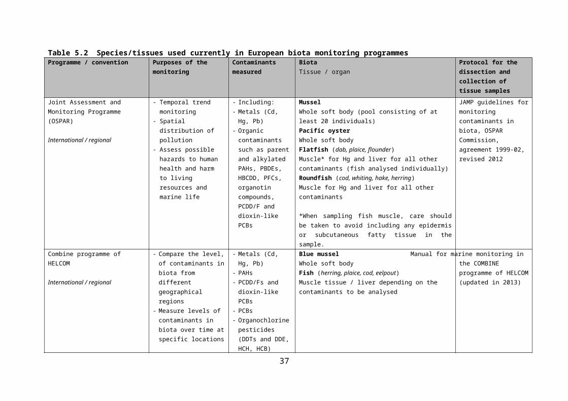
6. DATA HANDLING

6.1 Lipid and dry weight normalisationFor substances that accumulate through hydrophobic partitioning into the lipids of organisms, measured concentrations in biota can be normalised to fish with a lipid content of 5% (EC 2011a). This "benchmark" lipid content of 5% has been incorporated in the OECD 305 guideline for bioconcentration to ensure comparability between results of bioconcentration tests. The rationale behind this lipid normalisation is that the whole body biota concentration is linearly correlated with the lipid content of the species.

For a substance that does not accumulate by hydrophobic partitioning into lipids, but via another mechanism of accumulation, the lipid normalisation should be replaced by normalisation against another parameter, such as dry weight (e.g. mercury). The appropriate metric to use for normalisation will usually follow from the normalisation used in the bioaccumulation studies used to derive the standard. The "benchmark" dry weight content for fish is 26% (Smit 2005; EFSA 2009).

Other taxonomic groups, such as mussels, have different lipid and dry weight contents to fish. For mussels, EFSA has suggested a "benchmark" dry weight

38




Data Handling




content of 8.3% (Smit 2005; EFSA 2009), and the energy content for mussels of 19.3 kJ/g dw (Smit 2005; EFSA 2009) corresponds to a lipid content of approximately 1% for freshwater and marine bivalves (Bruner et al. 1994; Lazzara et al. 2012; Pleissner et al. 2012).

Thus, the values of 5% lipid weight and 26% dry weight content for fish, and 1% lipid weight and 8.3% dry weight content for mussels, should be used as the benchmark for normalising contaminant concentrations on a lipid or dry weight basis for assessment against the relevant biota standards, where appropriate. This requires that the actual lipid and/or dry weight content of the sampled biota are determined alongside the contaminant concentrations, or that generic values for the particular biota species are used, such as those available in FishBase6.

Normalisation of measured concentrations in biota to the benchmark lipid or dry weight contents may be used as a regulatory tool to harmonise compliance assessment across Member States, but is not suitable for local risk assessment.

Normalisation of measured data to lipid content and dry weight is described in A.7.

6.2 Trophic LevelThe biota standard should be applied to the most ‘important’ link in the food chain. In this context, ‘important’ means the trophic level where concentrations peak, such that the predator of species of that level is exposed to the highest food concentrations. In general, for substances subject to biomagnification, the critical concentrations are attained at trophic levels (TL) 3 to 4 in freshwater food webs, and TL=5 for marine food webs.

There are, however, exceptions to this general rule. For metabolisable substances, such as PAHs, invertebrates (at lower trophic levels in the food chain than TL = 3-4), may accumulate these substances to a higher extent than vertebrates such as fish7. In this case the quality standard should be derived for the specific food web that depends on invertebrates such as mussels at its lower levels (i.e. TL = 2), and may not involve fish at all (e.g. water»algae»mussels»diving ducks). The biota standard for PAHs is therefore expressed as a concentration in mussels (in order to protect mussel eating predators).

Because of the different bioaccumulation potential of substances across different species classes, the biota standards for brominated diphenyl ethers, hexachlorobenzene, hexachlorobutadiene, mercury, dicofol, perfluorooctane sulfonic acid, dioxin and dioxin-like compounds, hexabromocyclododecane, and heptachlor and heptachlorepoxide refer to fish (and for dioxins and dioxin-like compounds fish, crustaceans and bivalves), and the biota standards for fluoranthene and the PAHs refer to crustaceans and molluscs (Table 1.1).

6 http://www.fishbase.org/7 Not all fish metabolise PAHs (e.g. most catfish species do not)

39

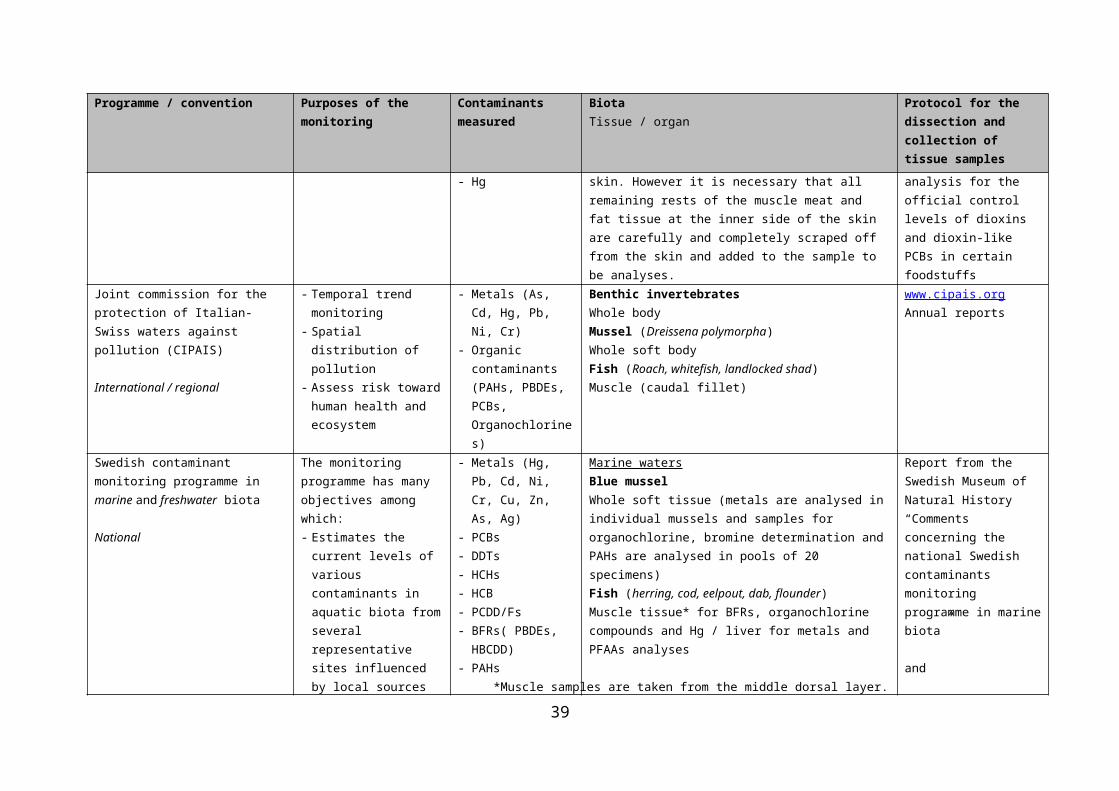
Directive 2013/39/EU (EC 2013) states that an alternative biota class, or another matrix, may be monitored instead of the specified biota class, as long as the EQS applied provides an equivalent level of protection. This implies that if, for example, a monitoring program with mussels (TL = 2) or fish from lower trophic levels is implemented, this might be used for comparison with the biota standards. In such cases, the EQSbiota needs to be adjusted according to the monitored trophic level.

Data on the trophic level of the diet is lacking or not well-known for most European avian and mammalian predators in the aquatic environment, especially for freshwater. From stable isotope measurements, it appears that the avian and mammalian predators in the food web do usually not exceed trophic levels of 4.5 and thus feed on trophic levels of 3.5 (on average). The top predators in the marine food chain may have trophic levels of 5.5 or higher. Therefore, the trophic level of species in which EQSbiota are monitored can be considered to be sufficiently protective if they represent levels of 3.5 and 4.5, respectively for the freshwater and marine environments.

When human fish consumption is considered, fish at trophic level 4 seems a reasonable estimate for the fish species that are generally consumed by humans. The median trophic level for European fish species for which commercial fisheries exist is 3.8 (Fishbase8), but most of these are marine species. This is probably an indication that fishery products that are consumed by the general population originate largely from marine sources and not from freshwaters. The quality standards for freshwater should, however, also protect subgroups of the European population that consume higher amounts of fish that are retrieved locally from freshwater sources, e.g. the angler or those living in areas adjacent to great lakes or rivers.

Trophic positions are not fixed values for each species, but may vary from one ecosystem to another and even from one individual to another. For example, eel from two lakes from Germany and Denmark were shown to have completely different feeding habits, from almost completely piscivorous to completely benthivorous, leading to a difference of one trophic level, both on the basis of stomach contents and based on stable isotope analysis (SIA) (Dörner et al. 2009). The trophic level of pikeperch (Sander lucioperca), pike (Esox lucius) and European catfish (Silurus glanis) in two small rivers in France were 0.7, 0.9 and 0.7 times higher in one river compared to the other, based on stable isotope data (Kopp et al. 2009). Therefore, it is recommended to determine the trophic level of the sampled biota together with the analysis of the pollutants.

Preferably, the trophic position is determined by measuring stable isotopes in the biota samples, of which the enrichment in nitrogen isotope ratio (δ15N) is a measure of trophic position. This method has been proven to provide estimates of the trophic level (e.g. Vander Zanden et al. 1997; Jardine et al. 2006). The determination of trophic levels by this method forms the basis of most of the trophic magnification studies, in which the accumulation of substances in a food 8 www.fishbase.org

40

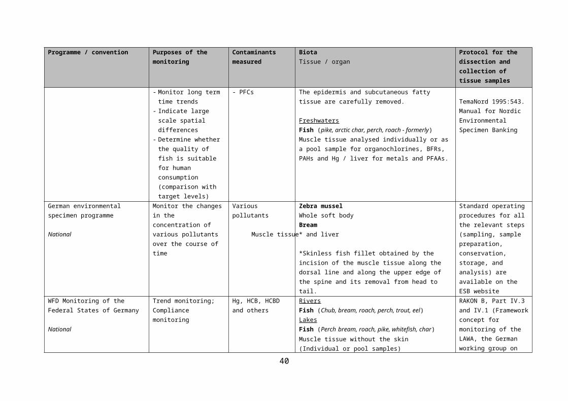
web are studied. Determination of the trophic position of any given biota should also involve the characterisation of a baseline of a particular food-web (based on measurements on primary producers or consumers).

Methods for determining the trophic level of sampled biota, and for converting EQSbiota between different trophic levels are given in Annexes A.8 and A.9.

41

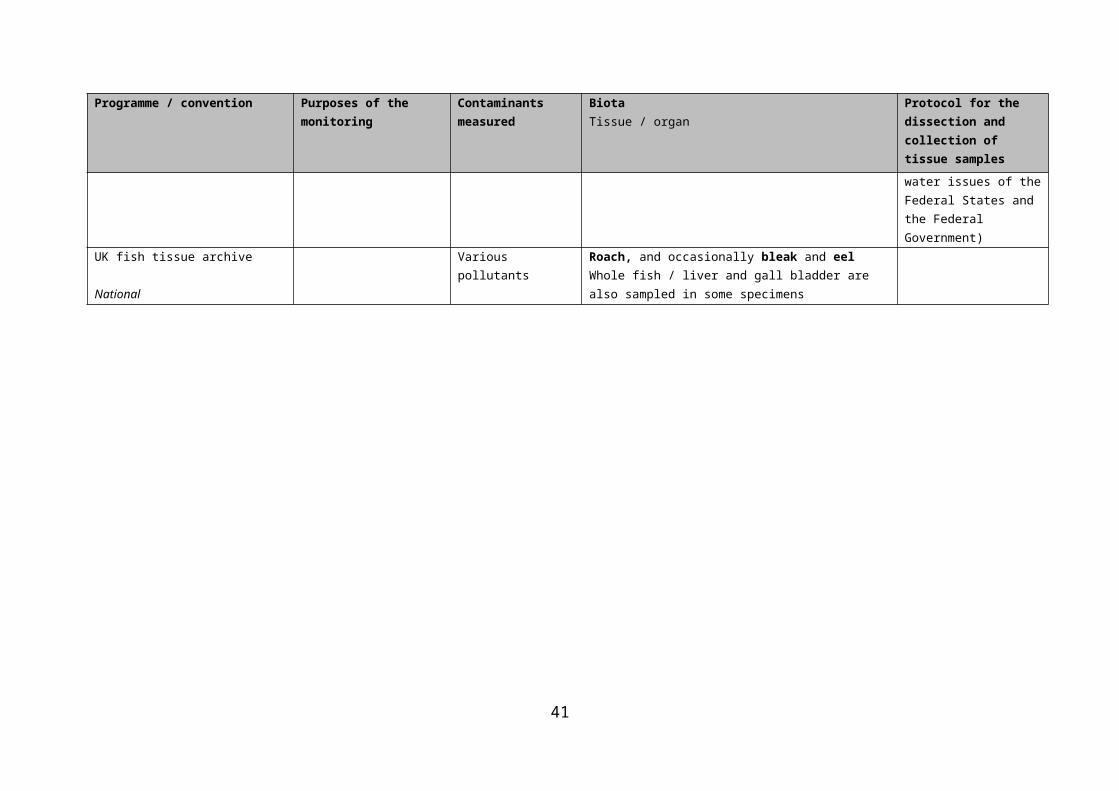
7. ASSESSING COMPLIANCE WITH A BIOTA EQS

7.1 Using measured chemical concentrations to determine compliance

Compliance is determined by comparing the chemical residue data measured in biota taken from a site with the EQSbiota, following normalisation (where required/ applied – Section 6) and log-transformation. The mean of the log-transformed chemical residue data is the statistic used for comparison with the EQSbiota.

Assessing compliance with biota standards is subject to the same statistical considerations as any other standard, and these are covered in ISO guidance on the use of sampling data for decision making – compliance with thresholds and classification systems (ISO 2008).

42

Look in:ISO (2008) International Standard 5667-20 Water Quality – Sampling Part 20: Guidance on the use of sampling data for decision-making – compliance with thresholds and classification systems.




Data Handling




Decisions about compliance with the standard may be undertaken on the basis of a ‘face value’ assessment (comparing the mean of a number of samples with the EQS), or statistical approaches that take account of uncertainty in measured values. These are required if the assessment of compliance is to be supported by an estimate of the confidence in the decision (i.e. whether a site has passed or failed the EQS). Thus, a ‘fail safe’ decision can be made in which a decision is made on the basis of an upper confidence interval (the effect of uncertainty is to give the benefit of doubt to the environment but false positives are more likely) or, alternatively, the pass/fail decision is made on the basis of the lower confidence interval (false negatives are more likely).

7.2 Estimating confidence in compliance assessments Statistical approaches require an estimate of the variability between samples and this is typically undertaken by estimating confidence limits around the summary statistic (in the case of biota standards, the mean). However, biota monitoring allows no estimate of temporal variability to be made, and the only available information on variability relates to that between replicate fish (i.e. fish sampled from the same location, at the same time).

To properly understand variability at a location, biota samples taken on each sampling occasion should not be pooled9. However, resource constraints may encourage pooling of samples to reduce the amount of analysis needed. Pooled samples give a reasonable estimate of the mean concentration (the compliance statistic) but information about variability is lost. This means the confidence of the comparison with the EQS (i.e. pass or fail) cannot be assessed (unless the biota body residues are much higher or lower than the EQS) and this could reduce the regulators’ ability to take action. If individual samples cannot be analysed separately, information about variability between individuals may be obtained from samples taken in previous years or from locations that are subject to similar chemical pressures, and support similar fish stocks.

The total variability depends on individual variability, analytical variability and also between-year variability, if data from more than one year are included in the analysis. When variability is high, more samples will be needed to provide a reasonably confident estimate of the mean than when there is close agreement between samples (Section 4.2.1). The variability is indicated by the statistical distribution of measured concentrations of chemicals and by statistics like the standard deviation, or the 5th and 95th-percentiles.

9 It may be necessary to combine several fish into a sample to get enough material for analysis. The point remains the same though – there must be several samples in order to determine confidence in pass/fail decisions.

43

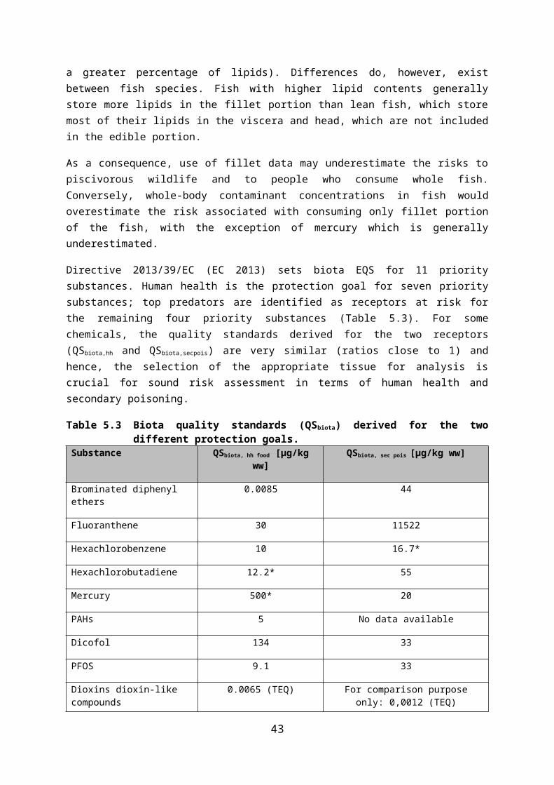
7.3 Assessment periodIn terms of the period over which compliance against the EQS should be assessed, there are at least two options that could be applied and these are presented below. It is important that there is a clear understanding of the limitations of each option before commencing sampling.

a) Assessment of compliance on an annual basis10.

Year 1 Year 2 Year 3XXXXXX

XXXXXX

XXXXXX

Compliance assessment based on mean



Or

b) Assessment of compliance after three years (assessment of compliance once in a three-year rolling system). Compliance assessment based on pooled data (to estimate a three-year mean) can then be re-assessed each year using the last three years’ data.

Year 1 Year 2 Year 3XXXXXX

XXXXXX

XXXXXX

Compliance assessment based on pooled data to estimate ‘three-year mean’

10 Each ‘x’ refers to a sample as defined in Section 2.1.1, Footnote 1.

44

Individual samples used to estimate mean (and confidence limits)






ANNEXESA.1 Steps applied for the selection of biota for a

monitoring programme in France (2011-2013)A.1.1 Background

Due to specific concerns about fish contamination and human health, a PCB (polychlorinated biphenyl) action plan was implemented in France between 2008 and 2013. This plan aimed, among other objectives, to gain an extensive view of freshwater fish contamination. Data on other contaminants, in particular mercury (Hg), hexachlorobutadiene (HCBD), hexachlorobenzene (HCB) polybromodiphenlyethers (PBDEs) and perfluorooctane sulfonate (PFOS) were also collected. Besides the primary goal of assessing fish contamination by PCBs, these data were used in support of the design of the biota monitoring programme in France (Babut et al. 2013).

A.1.2 Step 1: Accumulation potential

At this stage, HCBD and HCB were not considered because they were seldom detected, other than at a limited number of sites. Several statistical approaches (e.g. cluster analysis, ANCOVA) were used to classify fish species in several groups according to their accumulation potential based on available data and information from scientific literature.

The accumulation potential of these species was tested for other contaminants, with methods adapted to the available data. The influence of species selection on the probability of exceeding the EQS was tested for PFOS, whereas for PBDEs a principal component analysis helped to map the species’ accumulation potential.

A.1.3 Step 2: Matching the accumulation potential with fish availability

This was first investigated based on the fish contamination database. River typology (lowlands versus mountainous areas) was also considered at this stage, as well as fish mass (i.e. the availability of fish individuals exceeding a given mass in the database). In this example the mass threshold was primarily set at 300 g, because it was intended to sample only fillets. This value of 300 g was required by contract laboratories, but could certainly be lowered, in particular if the requirement shifted to the analysis of whole body instead of fillets (Table A.1.1).

45

Table A.1.1 Most frequently sampled species in France (2011-2013).

Species

Abundance

Spatial range

Accumulation potential

Individuals≥ 300 g?

PCB, dioxins, furans

PBDE PFOS

eel medium medium + high high high

barbel high large in plain + high low high

common bream

low large rivers, lakes/ponds

+ high low high

pike low large rivers, lakes/ponds

+ low medium medium

chub high large in plain + medium-low

low low

perch medium-low

large, incl. lakes/ponds

low medium high

trout medium upstream reaches

medium medium high

Note that there were many other species in the database, but they were not well distributed throughout the sampling sites.

A.1.4 Step 3: Species selection

It was decided to recommend 2 species in order to circumvent sampling contingencies, and as a compromise for varying accumulation potential. Based on the table above, the most suitable species (for this range of contaminants) were eel, barbel, and chub.

The eel was discarded because of concerns about its abundance. The river trout was added to the list for the monitoring of upstream, fast flowing reaches.

The bream was recommended as an alternative option to the barbel (in case of absence of this species). Similarly, the perch was recommended as an alternative to chub.

A.1.5 Step 4: Feasibility check

A GIS11-based analysis of species availability was implemented on the basis of the database resulting from ecological monitoring. The applied criteria were as follows: (a) presence of chub, barbel, trout, perch or bream; (b) 7 to 9 individuals weighing ≥ X g and (c) at least once in the period 2007-2011.

11 Geographical information system46

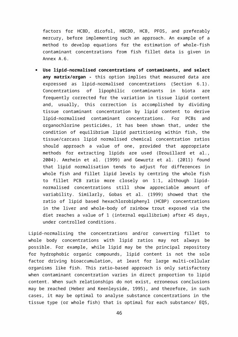
The number of individuals was derived from the above mentioned study (Babut et al. 2013), based on a simulation of the probability of exceeding the EQS as a function of sample size. In this case, 7-9 individuals allow a probability of 80% to predict an exceedance of EQS with less than 20% error. Several scenarios were tested for fish mass (Table A.1.2, Figure A.1.1).

47

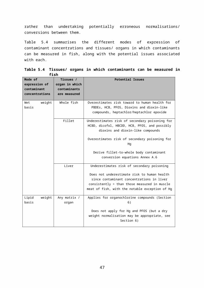
a- Chub (S. cephalus) sites

b- Trout (Salmo trutta fario) sitesFigure A.1.1 Maps showing the sites matching the project criteria

Table A.1.2 Species, sample size and mass scenariosSample size

9 individuals 7 individuals

Fish size ≥300g ≥200g ≥150g ≥300g ≥200g ≥150gBarbel 72 95 130 98 130 167Bream 9 13 21 16 21 28Chub 198 320 431 287 414 544Perch / / 3 / 2 7Trout 70 111 259 106 159 321Total (N sites)

312 476 719 442 617 879

From this analysis, the use of perch as an alternative species appeared questionable owing to its low abundance. The added value of the bream might also be further assessed (i.e. test whether bream are present when barbel are absent).

48

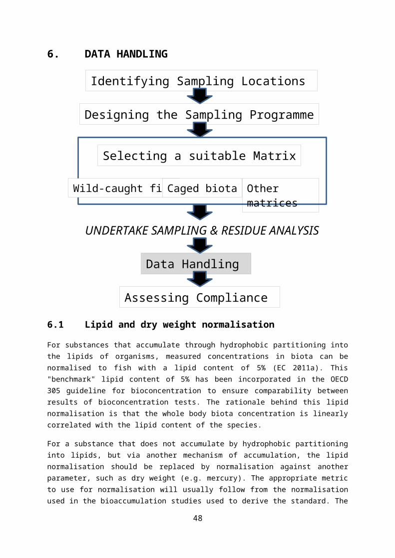
A.2 Using trend monitoring data to assess EQS compliance

Due to the difference between surveillance and operational monitoring, and their required associated monitoring frequencies, the period with monitoring data available for compliance assessment will vary between different water bodies. For some water bodies there may only be data available for one single year for the assessment of compliance, e.g. water bodies only covered by surveillance monitoring and with concentrations less than the EQSbiota. For water bodies subject to operational monitoring there will be yearly data available for some priority substances whereas, for substances identified as substances behaving like ubiquitous PBTs, there might only be data from every third year.

There will therefore be a need to be able to assess compliance, based on data covering different periods of time. In order to assess compliance based on all the available data, and if no statistical temporal trend can be seen, the entire time period with available data could be used to evaluate compliance. This reduces the effect of between-year variability. In Figure A.2.1, yearly monitoring data are available for 13 years and there is large between-year variability. This variability could thus affect the outcome of the compliance assessment if based on data only from the last year, or the last three years. For example from Figure A.2.1, the geometric mean for a single year varies generally between 150 and 300 ng/g fw, whereas the geometric mean for the entire time period is 220 ng/g fw (although for compliance assessment the period over which compliance was measured would be shorter than in this example). Nevertheless, the recommendation here remains the same, i.e. use of the mean of measurements where possible.

49

Figure A.2.1 Time series of Hg concentrations in Perch from Lake Bysjön.

[Concentration in muscle tissue (ng/g fresh weight) on y-axis, year on x-axis. Each small dot represents an individual measurement and the larger dots the geometric means (Nyberg et al. 2013) from trend monitoring]

If the existing data reveals a statistically significant trend, the slope of the trend can be used to estimate the concentration for the last year. Figure A.2.2 shows, the geometric mean for the entire time period is 28.7 ng/g fw. There is however a statistically significant decreasing trend and the concentration estimated for the last year from the regression is 23.8 ng/g fw.

50

Figure A.2.2 Time series of Hg concentrations in arctic char from Lake Abiskojaure.

[Concentration in muscle tissue (ng/g fresh weight) on y-axis, year on x-axis. Each small dot represents an individual measurement and the larger dots the geometric means (Nyberg et al. 2013).]

51

A.3 Screening as an approach to developing a biota monitoring programme

In some cases it will be relevant to use a stepwise, screening or tiered approach to identify problem areas or major sources of potential exposures, before implementing a full biota monitoring programme (e.g. to assess compliance with biota standards).

In a tiered approach the relative concentrations in different areas of concern are first ranked using measured or modelled data for other compartments, and the outcome used to identify the areas where the highest concentrations can be expected. This allows a prioritisation for the assessment in a second tier, i.e. for the monitoring of concentrations in biota. Possible first tier approaches could be based on measurements in the water column, suspended matter, sediments or passive sampling (in water or in sediments), but not all will be appropriate for all situations.

A.3.1 Water

The selection of priority substances to be monitored in biota, as it is set in Directive 2013/39/EU, is partially based on difficulties to assess good status or trends in the water column. Assessment criteria derived and set for the water column (EQSs) are very low, often lower than the LOQ of available analytical methods, and the results very variable due to a strong variation in the content of suspended matter to which the substances associate. As a consequence, data on water concentrations that could be used in a first tier assessment will be limited. Even when it is available, water concentrations may not always relate to biota concentrations and there is a risk that of overlooking what may be found in biota.

If the EQSbiota is to be converted to a concentration in water, the most reliable metric for the recalculation are field derived bioaccumulation factors, normalized to standard lipid content (or dry weight content). Because bioaccumulation factors are also dependent on the trophic level, the preferred assessment is to make a linear regression of log BAF versus trophic level and determine the BAF at trophic level 4. The application of a single trophic magnification factor as the biomagnification factor in the aquatic food chain appears to be insufficient, at least for hexachlorobenzene, i.e. the multiplication of the laboratory BCF with the field derived trophic magnification factor failed to accurately predict the bioaccumulation in the field. It appeared that the difference between this bioaccumulation factor at a trophic level of 4 and the bioconcentration factor, both determined in fish, was very close to the trophic magnification factor to the power of three (Moermond and Verbruggen 2013). If reliable bioaccumulation data are missing, the bioaccumulation factor at trophic level 4 could provisionally be estimated from the bioconcentration factor and trophic magnification factor, if reliable values for these parameters are available. That is:

BAF(TL = 4) = BCF x TMF3

52

At the same time, it can be concluded that in the absence of biomagnification, BAF will not be dependent on trophic level and will be approximately equal to the laboratory derived BCF.

A.3.2 Suspended matter

Because suspended matter (SPM) can be considered in equilibrium with the water phase in the water column, concentrations in SPM will reflect environmental quality. Via the equilibrium partitioning (EQ) theory (DiToro 1991) organic carbon based concentrations can be used for ranking the areas or may even allow an a priori conversion to lipid-based biota concentrations for low trophic level organisms. An overestimation of the concentrations is not very likely, as SPM may contain black carbon (e.g. soot), that often demonstrates higher sorption power than what is assumed in the classic equilibrium partitioning approach. SPM collection should be performed using flow-through centrifuges to obtain sufficient material for analysis. Clearly this approach is not applicable for rivers were SPM is absent, e.g. in rivers fed from glacial areas.

A.3.3 Sediment

The approach for SPM basically also applies to sediment although the organic carbon content is often lower and the relation to the concentrations in the water column is less obvious. Nevertheless the sedimentation over time also makes that the results may have an integrative nature.

A.3.4 Passive sampling

Passive samplers can also be used as a first level tier (Annex A.4) in water as well as in sediment. From the uptake of pollutants by passive samplers the freely dissolved concentration is estimated, which represent the driving force for bioconcentration. Thus, passive samplers enable the in situ determination of hydrophobic bioaccumulative organic compounds exposed to organisms at the lowest trophic level. Like organic carbon-based concentrations, the results from passive sampling can also be converted to lipid-based concentrations for an organism considered at equilibrium with the environment to which the sampler was exposed. This is similar to the approach for sediment but without having to account for the variable nature of organic carbon.

A.3.5 Models

Assuming data from the matrices described above are available, models can help us to understand the spatial and temporal variations in chemical concentrations. For example, measurements in sediments, biota and/or passive samplers can be combined in models and can be used to estimate dissolved water concentrations for some contaminants, particularly hydrophobic organic compounds, and vice versa. When such models are validated and tested they can provide, within the impact and pressure assessments, additional evidence that the EQS will not be violated in a specific waterbody even under the most adverse conditions (i.e. in the worst case exposure scenario), even if the monitoring in biota failed for

53

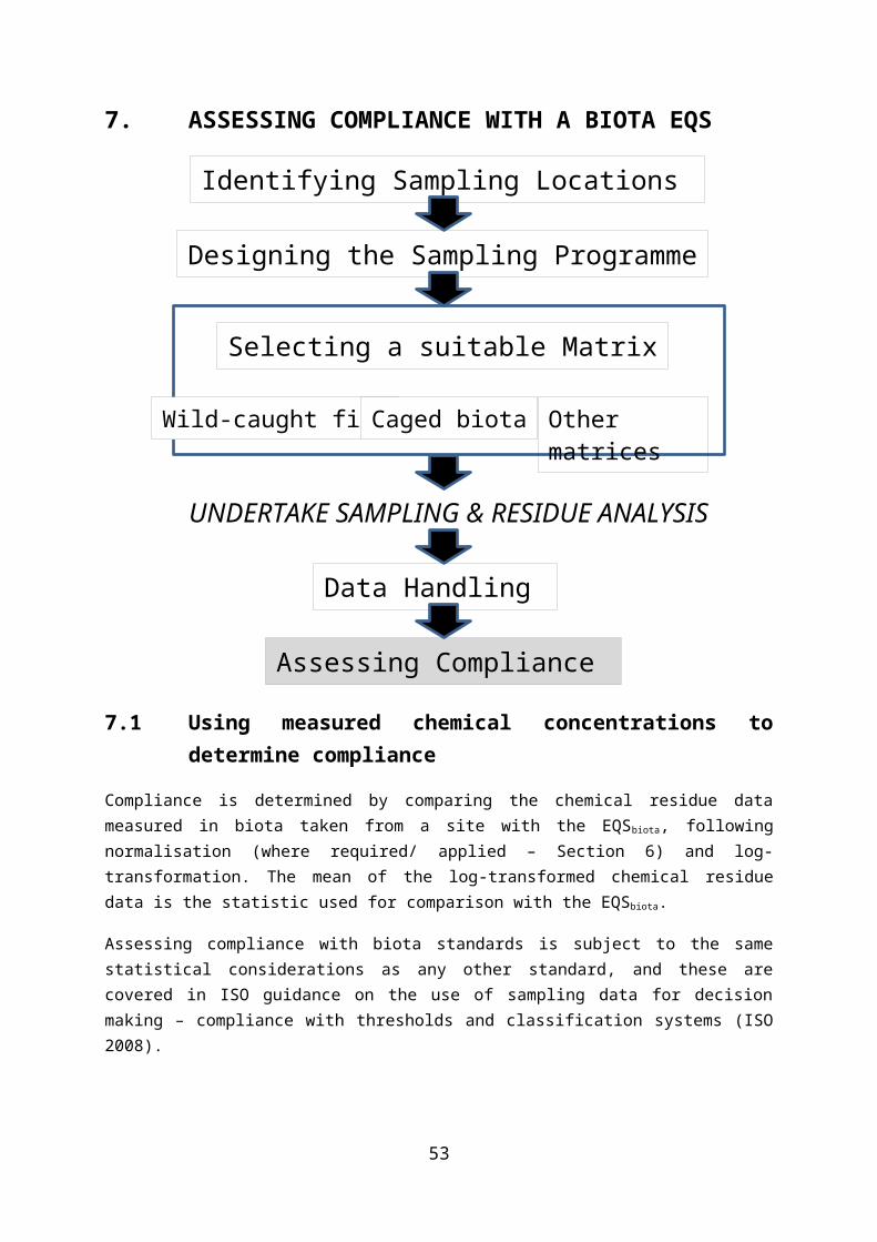
various reasons (e.g. because of limited availability of organisms with desired parameters for monitoring).

The predictive power of a model is only valid within the framework and limits defined by its assumptions. It is important to define the desired level of confidence and consider uncertainties associated with chemical measurements in biota/sediments/passive samplers/water as well as to other parameters used in the model.

A.3.6 Conclusion

The tiered approach is recommended in the first instance to identify areas where monitoring of biota is most important; i.e. the areas of potential EQSbiota

exceedance. These areas should be then subjected to a regular biota monitoring to assess compliance with the regulatory criterion (EQSbiota).

The first tier of monitoring (using the approaches described above) can also be continued in parallel with the execution of the regular biota monitoring programme. The parallel monitoring in different matrices (e.g. passive samplers and biota) allows the gathering of more evidence and information on quantitative relations between chemical concentrations found in the monitored matrices. After a sufficient validation of these relationships it may be possible in future to reduce the monitoring efforts and switch the monitoring to the matrix which is more cost effective. Such an approach could be applied especially in areas where a good status has been shown previously and only the confirmation of no deterioration of the status is required (surveillance and trend monitoring).

54

Look in: Guidance Document No. 19 – Guidance on Surface Water

Chemical Monitoring under WFD, 4.3 Guidance Document No. 25 – Guidance on chemical

monitoring of sediment and biota under WFD (2010), 7.1.2.

For the purpose of compliance checking for water bodies that are at risk of failing WFD provisions concentrations of contaminants estimated by modelling cannot be used, unless it is compared with an equivalent concentration in water that has been derived using validated bioaccumulation data. The approach can, however, be used in surveillance monitoring for estimation of concentrations in water bodies that are shown to be not at risk when the uncertainty of the model is considered.

A.4 Potential use of passive samplingPartition based passive samplers (PB-PSD) accumulate hydrophobic substances from water because of much better solubility of such substances in the sampler material compared to water. Consequently, hydrophobic substances with low solubility in water are strongly accumulated in PB-PSD, which makes passive sampling a suitable method for monitoring the level of substances in the water phase. Samplers are made from hydrophobic polymeric materials with high permeability for the compounds to be sampled such as low density polyethylene (LDPE) filled with lipid (semi-permeable membrane devices, SPMD; Huckins et al. 2006) or without lipid (Adams et al. 2007), silicone rubber, i.e. polydimethylsiloxane (PDMS) based materials (Smedes, 2007), and polyoxymethylene (Cornelissen et al. 2008).

When, during exposure, passive samplers reach equilibrium with the surrounding water, concentrations in the samplers at various sites or different periods are, in principle, directly comparable and enable identification of concentration gradients or time trends. It is, however, more common to estimate freely dissolved aqueous phase concentrations (Cfree) from the equilibrated concentrations in the PB-PSD using the sampler water partition coefficients (KPW). This accords with the practice applied for more hydrophobic substances with log KPW’s larger than about 5 that do not attain equilibrium over typical exposure periods (2-8 weeks).

For these more hydrophobic substances the sampler capacity is larger than is accumulated from the volume of water “extracted” by the sampler during exposure. Consequently the estimated Cfree relies on the in situ estimation of the water volume extracted by the PB-PSD during the exposure period. This volume (or the sampling rate, when expressed per time unit) is derived from the release of selected substances (performance reference compounds, PRCs) dosed to the PB-PSD prior to exposure. Basically, the rate of release, controlled by the diffusion through the water boundary layer at the sampler surface, is determined. The first order rate constant of the release under the given sampling conditions (temperature and turbulence) is used for calculating the sampling rate. Subsequently the Cfree can also be estimated in situations when equilibrium is not attained (Booij et al. 2003, Huckins et al. 2006). Models for relating the sampling rate to compound properties have been developed (Rusina et al. 2010) as well as methods to estimate sampling rates (Booij and Smedes, 2010). Together with determined KPW values (Smedes, et al. 2009) the Cfree of the target compounds are derived from sampler uptake. These derived concentrations typically represent an average over a certain time period, often corresponding to the deployment period of the sampler (typically 2-8 weeks). It should be noted that there is no need to know the Kpw for the estimation of Cfree for very hydrophobic compounds that remain far from equilibrium.

Uncertainties in results obtained by application of PB-PSDs are believed to range around a factor two depending on the level of experience of the laboratory (Allan et al. 2009). Different aspects of uncertainty are discussed in Lohmann et al.

55

(2012). An ISO standard has been published that specifies procedures for the determination of time-weighted average concentrations and equilibrium concentrations of dissolved organic, organo-metallic and inorganic substances, including metals, in surface water by passive sampling, followed by analysis (ISO 2011).

Assessment is best based on the estimated freely dissolved concentrations of substances in the water phase or the sediment porewater (Cfree). This freely dissolved concentration is a more stable parameter than a concentration measured in total water as the level is not influenced by variable amounts of the substance bound to dissolved and suspended particulate organic matter. C free is further considered to play a key role in chemical uptake by aquatic organisms. Cfree is proportional to the chemical activity (Mayer et al. 2003) and, if in equilibrium with surrounding environmental compartments, it also represents chemical activity of those environmental compartments, including the biota at the base of the food chain (Reichenberg and Mayer, 2006).

In addition to these partition samplers, adsorption-based samplers are also available that can accumulate the more hydrophilic organic substances such as PFOS, tributyltin compounds or mercury. However, the uptake process is not yet well understood, so translation of laboratory calibrations to the field is subject to larger uncertainties (Harman at al. 2012). In spite of these shortcomings, adsorption-based samplers can give valuable results with regards to substance screening to give an early warning for increasing concentrations. It could also be an alternative method in situations where the classical monitoring approaches have an insufficiently low limit of detection. However, no passive sampler suitable for the regulatory monitoring of mercury is currently available.

The primary potential application is the use of passive samplers in a tiered approach to assessing compliance with EQSbiota as outlined in Annex A.3.

A.4.1 Example of monitoring by passive sampling in concert with deployed mussels

The applicability of passive sampling for estimating biota concentrations was demonstrated for polychlorinated biphenyls and polycyclic aromatic hydrocarbons in the coastal area of the Netherlands (Smedes, 2007). Passive sampling was performed using polydimethylsiloxane (PDMS) sheets, better known as silicon rubber, following procedures basically equal to OSPAR/ICES guidelines (Smedes & Booij, 2012). For the assessment of pollutant concentrations, free dissolved concentrations were calculated from the passive sampling data. The volume of water sampled by the sampler is calibrated in situ through measuring the dissipation of performance reference compounds (PRC) dosed to the sampler prior to exposure. PRC are contaminant like compounds not occurring in the environment, e.g. isotopically labelled target compounds or PCBs not occurring in technical mixtures, selected to comprise a hydrophobic range (logKow 3.5 to 6.5). The concept is explained in Booij & Smedes (2010). Samplers

56

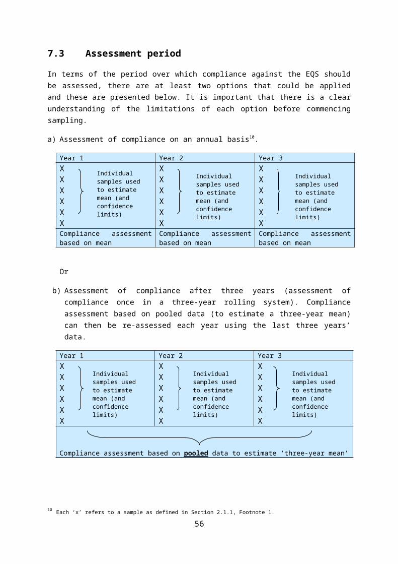
have been deployed in concert with the existing ‘‘mussel watch’’ programme in the Netherlands for over 12 years.

The monitoring program comprised 8 stations along the Dutch coast, where samplers and mussels were exposed for 6 weeks between November and February. Figure A.4.1 shows how, for fluoranthene, concentrations in water and mussels were closely correlated, demonstrating that the freely dissolved concentration measured with passive samplers is a very relevant measure for exposure of aquatic organisms at the lowest trophic level. The program did not include high hydrophobic priority substances but, as a representative hydrophobic substance, the data for PCB153 are plotted in Figure A.4.2, exhibiting the applicability for such compounds, even at a level of 20 pg/L (0.02 ng/L).

The seasonality observed in the mussels seems also to be reflected in the results from the passive sampling. The seasonal profile is likely to be related to a larger proportion of (more polluted) freshwater entering the areas monitored in winter compared to autumn, indicated by the lower average salinity in the winter periods. However, seasonality also occurs where there is little variation in salinity. A discussion whether correction for temperature and salinity are required is ongoing since seasonality effects on the passive sampling process may also influence accumulation by biota.

In conclusion, partition based passive sampling offers the possibility to screen for the presence of hydrophobic priority substances that tend to accumulate in sediment and/or biota. The assessment is usually based on the free dissolved concentrations of substances in the water column, averaged over time period of several weeks. Measured concentrations often correlate with those found in biota at the lowest trophic level.

0

1

2

3

4

5

6

7

0

20

40

60

80

100

120

140

160

180Fluoranthene

MusselWater

Figure A.4.1 A time series of Fluoranthene concentrations in the mid Western Scheldt for mussels

[µg/kg dry weight, gray dots, (left axis) and free dissolved concentrations in water determined through passive sampling (ng/L, open circles, right scale). Note that connecting lines are only to

57

guide the eye but do not represent intermediate concentrations. Measurements in mussels were ceased in 2007]

0

0.005

0.01

0.015

0.02

0.025

0.03

0.035

0

100

200

300

400

500

600

700PCB153

MusselWater

Figure A.4.2 A time series of PCB153 concentrations in the west Wadden Sea

[Mussels (µg/kg dry weight, gray dots, left axis) and freely dissolved concentrations in water determined through passive sampling (ng/L, open circles, right scale). Note that connecting lines are only to guide the eye but not represent intermediate concentrations.]

58

A.5 Quantity and preparation of biological material required for contaminant analyses

A.5.1 Quantity of biological material required for analysis

Biota EQS have been established for 11 priority substances with differing physico-chemical properties. Thus, a variety of different analytical methods have to be carried out on tissue samples to quantify the full set of substances, and this in turn implies that tissue samples are divided into as many sub-samples of lower mass as there are different analytical techniques that are used. Because EQS concentrations are extremely low for some of the priority substances, high sample volumes will be needed to meet the minimum performance criteria for chemical analysis, laid down by EC directive 2009/90. The tissue weight requirement for individual analysis will further depend on the species sampled, the available equipment, the method to be applied for chemical analysis, the concentration of contaminant in the sample and the lipid content (for lipophilic contaminants). It may be necessary to pool bulk biota tissues, particularly in the case of fish livers and mussel and other shellfish tissues, in order to provide sufficient quantities of material for chemical analyses or to save resources. Depending on species and size/age of fish, whole body or muscle tissue can provide sufficient amounts for analyses.

Tissue weight requirements for individual contaminant analyses are given in Table A.5.1. They reflect the current practice within ongoing national programmes for the monitoring of contaminants in biota. Overall, more than 100g wet weight of material (fish or bivalves) is required to analyse trace metals, PAHs and other organic contaminants. Figures are only indicative, however, since they may be representative of different monitoring purposes (trend and spatial analysis, compliance assessment, tissue archives for retrospective analysis), and as they may (or may not) include requirements for sample re-analyses. Additional tissue (sub)-sample should be reserved for the determination of dry and lipid weights and stable isotope (δ15N and δ13C) analyses.

Table A.5.1 Tissue weight requirements for contaminant analyses specified in monitoring programmes using biota for pollution assessment.

Programme Tissue / organ

Individual (I) or composite (C)

sample

Contaminant / parameter analysed

Weight(g, on a

wet weight basis)

Swedish contaminant monitoring

programme in marine biota

Fish muscle tissue I

Organochlorines and BFRs 10

PCDD/Fs 20

Mercury 1.5

Fish liver I Trace metals 0.5-1

PFAAs 0.5

59

Blue mussel whole soft

body

I Trace metals

C (20 individuals)Organochlorine

s, BFRs and PAHs

Irish national programme for the monitoring

of contaminants

in fish and fisheries

products under the WFD

Whole fish

C (whole fish homogenates comprising a

minimum of 10 individual size-classed

fish)

Organochlorine pesticides

(including HCB and HCBD)

5

BFRs 5

PCDD/Fs, dioxin-like

PCBs, indicator NDL PCBs

25

Mercury 5

Trace metals 10 (freeze dried)

Whole soft body of blue

mussels

C (minimum of 50 mussels, general size

range 4-6 cm)

Organochlorine pesticides 5

BFRs 5

PCDD/Fs, dioxin-like

PCBs, indicator NDL PCBs

25

HCB 5

HCBD 5

Mercury 5

Trace metals 10 (freeze dried)

PAHs 5

Flanders (Belgium eel

pollution monitoring

network (1994-2009)

Fish muscle tissue I

Organochlorine pesticides, PCBs

and BFRs10

PCDD/Fs 5

Metals 10

PFOS 2

VOCs 10

Flanders (Belgium) pilot

Fish muscle tissue (eel

C POPs and 10

60

study on monitoring in biota (2013-

2014)

and perch) metals

Fish liver C Metals 1

Whole soft body of mollusc bivalves

C PAHs 50

Spanish national

monitoring programme in marine biota

Fish muscle tissue I Mercury 1.5 (or 10-

15)

Fish liver

I Trace metals (except Hg)

1.5 (or whole liver)

I (if possible; use composite sample if

individual liver weight is too low)

Organochlorine pesticides and

BFRs2.5 (or whole

liver)


musselsC (minimum of 20

mussels)

Trace metals1.5 (or 200-300 for all analyses)

Organochlorine pesticides 10

BFRs 10

PAHs 10

Norwegian monitoring programme

MILKYS “Contaminants

in coastal waters of Norway”

Fish muscle tissue

I (if possible, otherwise pooled

samples)

Hg ?

Fish liver

Trace metalsPCB-7

Sum of DDTPBDE

HBCDDPFAS

Short-chain chlorinated

paraffins (C10-C13)

>50


mussels

I (if possible, otherwise pooled

samples)

Trace metalsMercury

PAHs (16)PCB (7)

Sum of DDTPBDE

HBCDDShort-chain chlorinated

paraffins (C10-C13)

>50

Austrian biota monitoring

Whole fish I (for trend monitoring)


15

61

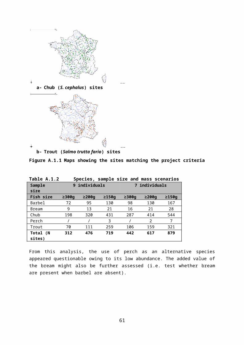
programme in running waters

C (for surveillance/complianc

e assessment)

Dicofol 20

PAHs (16) 20

Tributyltin compounds 10

PeBDE 10

HBCDD 15

PFOS 5

DEHP 10

Mercury 0.5 dry weight

PCDD/F, DL-PCB and NDL-PCB

25 g (dry weight)

UK national Clean Seas

Environment Monitoring Programme

Fish muscle tissue

Fish liver


mussels

C

C


BFRs (BDEs and HBCDD)PCDD/Fs

NDL-PCBs and DL-PCBs

10

PFAS 1

PAHs 20

Metals 10-20

Dutch contaminant monitoring

programme in marine biota Fish liver C

Organochlorines and BFRs 5-10

PFOS, PFOA 10

PCDD/Fs 5-10

Metals, moisture and fat content

5

Fish muscle tissue C

Mercury, moisture and fat content

10


mussels

C Metals, moisture, fat

content and ash30

Organochlorines and BFRs 70

PFOS, PFOA 10

PCDD/Fs 10-20

62

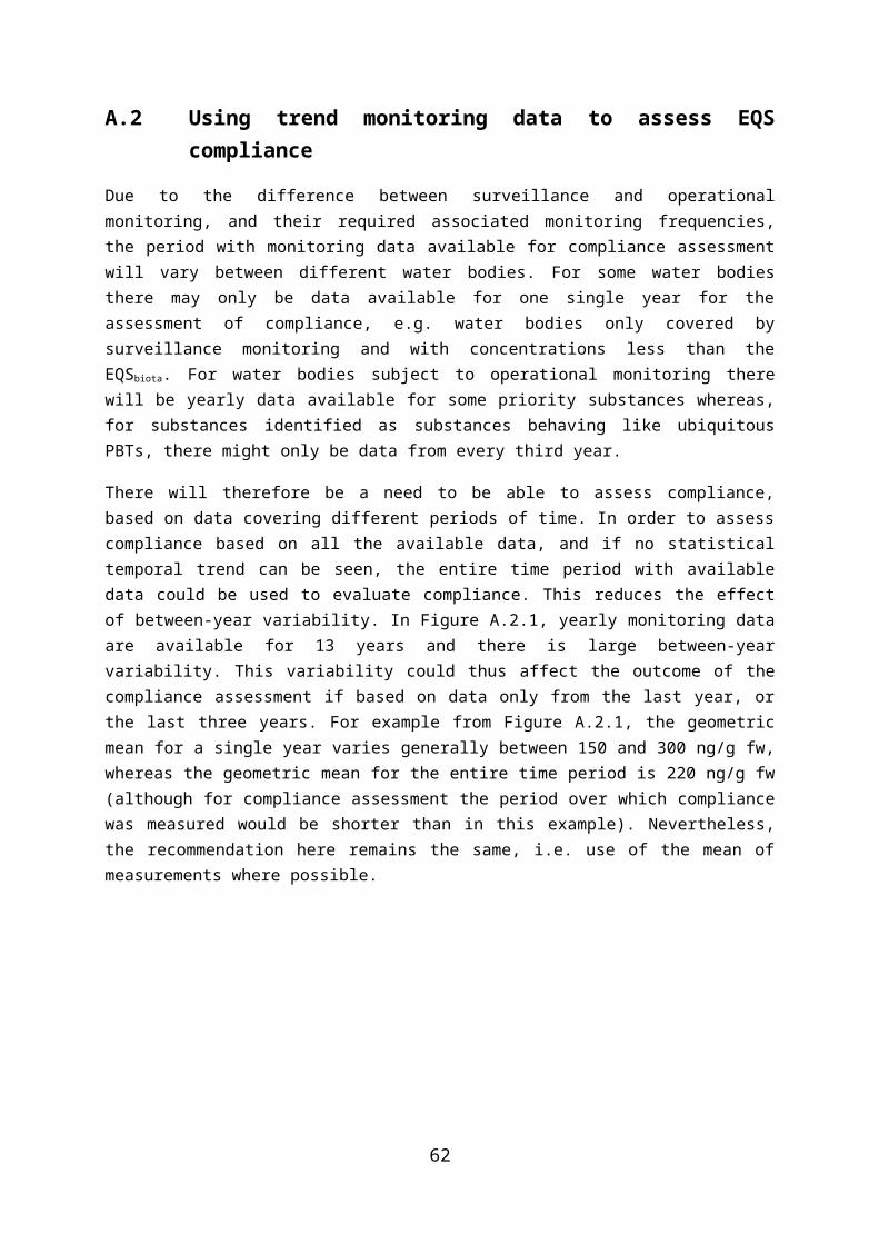
PAHs 20-40

Organotin compounds 15-20

Whole soft body of marine snails

C Organotin compounds 15-20

CIPAISInternational Commission

for the protection of Italian-Swiss

watersInternational /

regional

Fish muscle tissue C

Organochlorines, PCB, PAH;

PBDE> 50

Mercury > 50

Trace metals > 50

mussel whole soft

bodyC

Organochlorines, PCB, PAH;

PBDE> 20

Mercury > 20

A.5.2 Preparation of samples for whole body analysis (small fish and invertebrates)

Where small organisms (invertebrates or fish) are being used, the whole body (soft whole body for molluscs such as bivalve or gastropods) is generally used for chemical analysis.

Small fish should not be gutted, and bivalves should be allowed to depurate, prior to preservation and analysis, to remove their gut content, which is not representative of the contaminant body burden.

For gut purging the organisms should be placed in clean oxygenated water and left for 6-12 hours. The depuration time should be recorded. If possible, the depuration should begin immediately after sampling, but bivalves can also be transported alive to the analytical laboratory for gut purging.

Prior to depuration, bivalves can be stored in boxes (1 per station) and kept cool (at temperatures preferably <10°C) and damp (not in water) for up to 12 hours or for up to four days if the temperature remains <10°C. Adding damp seaweed (if available) to the boxes can help, otherwise they can be wrapped in clean humid woven fabric.

Transport of samples to qualified personnel for further preparation should be “over night” or, if frozen, by means that ensures that the samples will remain so. Agreement should be made with the qualified personnel prior to the time of shipment to ensure that the samples are properly received. Transport should

63

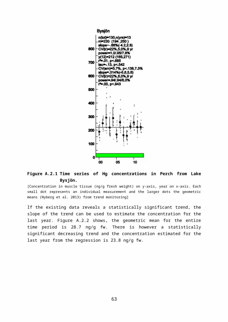
begin early enough in the week to avoid the risk that samples will still be in transit over the weekend. Samples should also be properly marked with the contact information of the recipient and the local contact, and the shipment should contain information on: station, geo-position, catch date, batch depth, species, catch method and any relevant comments.

Freezing may cause soft tissues to degrade and may result in uncontrollable losses of the determinants in the tissue or cross-contamination from other deteriorating tissues. If possible, frozen organisms should be thawed while ice crystals are still present in the tissues. Therefore, if samples have been frozen, they should not be allowed to thaw completely prior to dissection.

For molluscs with a shell, such as bivalves or gastropods, the whole soft tissues should be removed from the shell for chemical analyses. Bivalves should be shucked while still alive and avoiding tissue damage. Water contained within the shell should be allowed to drain away. This is especially important for bivalves collected in areas with high turbidity or on silt/clay bottoms. In such cases, whole tissues can be rinsed with clean seawater after being dissected. Soft tissue weight and shell length (or weight or volume) should be recorded in order to calculate the condition index. The removal of soft tissue from shells should be carried out immediately after the depuration period, otherwise they can be stored frozen at -20°C until dissection and analysis. The soft tissue samples should then be analysed immediately or stored at temperatures below -20°C.

A.5.3 Preparation of tissue samples (big invertebrates and fish)

If chemical analyses are not to be carried out on the whole body, dissection should be carried out immediately after collection. Field dissection and frozen storage of tissue samples is an option if suitable facilities are available (e.g. aboard a research vessel). Sub-samples of particular tissue should be removed and analysed immediately or frozen (temperatures below -20°C) until chemical analysis.

If it is not possible to dissect the organisms immediately, the whole organisms should be wrapped separately in suitable material and kept cool during transfer to the laboratory. Dissection should be undertaken within 24 hours of sample collection. However, if longer periods are required to transport samples un-dissected, organisms can be stored frozen at -20°C in appropriate containers. If possible, frozen organisms should be thawed while ice crystals are still present in the tissues. Therefore, if samples have been frozen, they should not be allowed to thaw completely prior to dissection.

Length and weight of whole fish need to be recorded in order to determine the condition of individual fish, and, during dissection of fish, biometric measurements should also be recorded (weight of whole liver and whole gonads, Section 5.3).

64

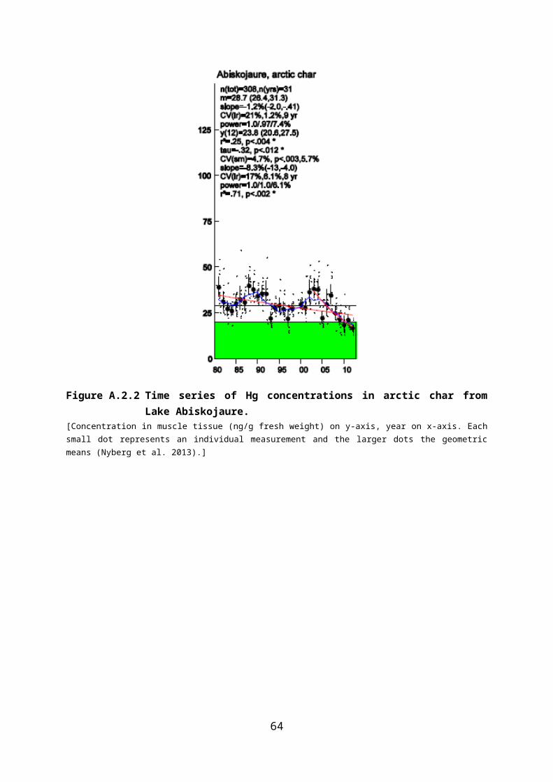
A.6 Estimating whole fish contaminant concentrations from tissue concentrations

A.6.1 An example of a method to develop equations for the estimation of whole-fish contaminant concentrations (excerpt from Bevelhimer et al. 1997)

In addition to analysing fillet portion (i.e. muscle tissue) for contaminants, the remaining carcass (i.e., whole body minus the fillets) of selected species are also analysed for the same contaminants. For the statistical analysis, sites are combined to provide a wide range of contaminant concentrations.

Whole-body concentration CWB is calculated as:

CWB = (CF×WF + CC×WC)/(WF + WC) (1)

where CF and CC are the contaminant concentration (µg/g) in the fillet and carcass, and WF and WC are the weight of the fillet (both sides) and carcass, respectively.

Alternatively, a standard fillet is taken from each fish and homogenised according to standard procedures. A subsample of this tissue homogenate is analysed for contaminants. Whole fish samples consist of the remaining fish portion after filleting and include the head, viscera and fins. The surplus tissue from the homogenised fillet sample is also added. All of this tissue is then combined and homogenised, and a subsample is analysed for contaminants. Because whole fish analyses are conducted on a sample from which (x) g of fillet material have been removed, whole fish results are likely to have a slight positive bias, with whole fish concentrations that are greater than fillet concentrations, and a slight negative bias when whole fish concentrations are less than fillet concentrations (Amrhein et al., 1999).

Throughout the analysis, the following underlying model is used to relate whole body contaminant concentrations (CWB) and fillet concentrations (CF):

CWB = k’ + k×(CF)b (2)

where b>0 and k’ is assumed to be zero, resulting in a relationship that passes through the origin. For this reduced two-parameter model, taking logs on both sides of Eq. (2) changes the model to a standard linear regression model of ln(CWB) and ln(CF). Therefore all concentration values were natural log transformed for statistical analyses. For some applications, it might be reasonable to consider k’>0, in which case a nonlinear or weighted estimation method should be used to estimate the unknown parameters.

A logical progression of statistical tests is established to determine the most appropriate equation for the conversion of fillet concentration to whole body concentration for each contaminant (Figure A.6.1). This series of statistical tests is performed for each contaminant by species group. The first question addressed

65

is whether the measured fillet concentration is different from the calculated whole body concentration. A paired t-test is used to determine if the average difference of the fillet and whole body concentrations are different from zero (P < 0.05 for all analyses). If no significant difference is found, it is concluded that the fillet concentration can be used as the whole body concentration. If the difference is statistically significant, the analysis proceeds to the next step.

The second question addressed is whether the regression model

Ln(CWB) = ln(k) + b×ln(CF) (3)

produced a slope b, which differs significantly from 0. If the slope is not different from zero, it is determined that the existing data are not adequate to derive a reasonable relationship for that contaminant. If the slope differs from zero, the evaluations determine whether it differs significantly from 1. If the slope does not differ from 1, then the following equation is used to define the relationship between whole body and fillet concentrations:

CWB = k×CF (4)

where k is the mean whole body-to-fillet ratio as estimated from the antilog of the mean difference of the logs; i.e.

ln(CWB) minus ln(CF) for each analyte by species combination.

If the regression analysis reveals that the slope is significantly different from 1, the estimated model is then used as shown in Eq. (3) to define the conversion equation. A stepwise regression analysis is also performed to determine if whole-body weight (or fish length) and fillet lipid content are significant explanatory variables in addition to the fillet concentration for predicting whole-body contaminant concentration.

A.6.2 Limitations and uncertainties to be considered

Due to the lack of studies suggesting otherwise, the above analysis is limited to a single model type where the y-intercept passes through the origin. This model includes two forms: one linear and the other curvilinear. However, it is possible that for some contaminants a different model form would be a better descriptor. For example, it may be the case for some chemicals that the y-intercept does not intersect the origin. Moreover, a different model form would be required if whole body and fillet concentrations converge at high concentrations. The model given by Eq. 3 has the capability to handle these cases when k’>0.

Other limitations of the conversion equations presented here include variations in within-body contaminant distribution among fish of different sizes and species. As fish grow, changes are expected in the proportion of the body made up of muscle, the distribution of lipids, and the apportionment of energy and contaminants to reproductive tissue. For similar reasons, differences are expected among sexes. Among-species differences exist in physiology, body structure and lipid apportionment; therefore, differences in the fillet-to-whole

66

body contaminant relationships among species are possible. For example, the ratio of whole body to fillet concentrations of hydrophobic contaminants would be expected to be higher in species that store much of their lipids in the peritoneal cavity than other species which store a greater proportion of lipids in muscle tissue.

Figure A.6.1 Flow diagram describing statistical procedures used to determine equations for estimating fish contaminant concentrations from fillet values (redrawn from Bevelhimer et al. 1997).

[CWB: Whole-body contaminant concentration; CF: Fish fillet contaminant concentration.]

67

A.7 Normalisation of measured dataThe appropriate metric to use for normalisation of contaminant concentrations in biota will usually follow from the normalisation used in the bioaccumulation studies used to derive the biota EQS.

For substances that accumulate through hydrophobic partitioning into the lipids of organisms, measured concentrations in fish should be normalised to fish with a lipid content of 5% (EC 2011a). The energy content for mussels of 19.3 kJ/g dw (Smit 2005; EFSA 2009) corresponds to a lipid content of approximately 1% for freshwater and marine bivalves (Bruner et al. 1994; Lazzara et al. 2012; Pleissner et al. 2012), and measured concentrations in bivalves should therefore be normalised to bivalves with a lipid content of 1%. The rationale behind this lipid normalisation is that the whole body biota concentration is linearly correlated with the lipid content of the species for those substances.

For a substance that does not accumulate by hydrophobic partitioning into lipids, but via another mechanism of accumulation, normalisation against another parameter, such as dry weight (e.g. for mercury), may be appropriate. The benchmark dry weight content for fish is approximately 26% (Smit 2005; EFSA 2009). For mussels, EFSA has suggested a benchmark dry weight content of 8.3% (Smit 2005; EFSA 2009).

Based on the above, contaminant concentrations should be normalised to lipid contents of 5% in fish and 1% in bivalves, or to dry weight contents of 26% in fish and 8.3% in bivalves, on the basis of the measured lipid content or dry weight, or on the basis of generic values for lipid content or dry weight for the relevant species obtained from FishBase, for example.

To calculate the normalised concentrations cn, lipid or cn, dry weight from measured concentrations cmeas for a fish species x, the following equations can be used (lipid content and dry weight content expressed as mass fractions):

cn, lipid = cmeas · 0.05/lipid contentx

or

cn, dry weight = cmeas · 0.26/dry weightx

Similarly, to calculate the normalised concentrations cn, lipid or cn, dry weight from measured concentrations cmeas for a bivalve species x, the following equations can be used (lipid content and dry weight content expressed as mass fractions):

cn, lipid = cmeas · 0.01/lipid contentx

or

cn, dry weight = cmeas · 0.083/dry weightx

68

Using the exact lipid or dry weight content of the biota samples is always preferred over generic values for the species (such as those available from FishBase).

69

A.8 Trophic level determinationStable isotope determinations are not very demanding. However, for a good estimate of trophic levels the determination of stable isotopes for primary producers and/or primary consumers, occupying trophic level 1 and 2, respectively, together with the values for the biota samples, is required. Molluscs are filter-feeders and as such the δ15N values for these primary consumers (occupying trophic level 2) are very suitable as baseline value for the trophic food chain (post 2002). A value of 3.4‰ for the mean enrichment in δ15N per trophic level has been confirmed as a suitable value. The trophic level of a fish (or other) species can then be calculated according to the following equation (Vander Zanden et al 1997):

Trophic level = (δ15N(fish) - δ15N(mussel))/3.4 + 2

Although the mean enrichment value per TL of 3.4‰ has been used in most of the trophic magnification studies that are available, other studies suggest that a lower value might be more appropriate. For example, a value of 2.75‰ was recently proposed based on an analysis of data for mammals, birds, fish and invertebrates, and their diets (Caut et al 2009). Using a lower value would lead to a higher trophic level. Because most trophic magnification factors (TMF), which are factors describing the average biomagnification of a substance per trophic level, are based on values of 3.4‰, it is advised to use this value in the calculation of tropic levels.

70

A.9 Trophic level conversionBecause of the widespread environmental occurrence of priority substances, many field bioaccumulation studies have focused on these substances. For most of the priority substances for which a biota standard has been set, multiple field bioaccumulation studies are available. These data are essential to make a translation from a standard in one type of biota (e.g. fish) to another (e.g. mussels) and from the biota standard into an equivalent concentration in water.

The trophic magnification factors that should be used for this purpose are trophic magnification factors that refer solely to the pelagic food chain, so excluding birds and mammals. Biota samples will be restricted to pelagic species and, therefore, only the relative accumulation in species in the pelagic food chain is relevant. The extra magnification step in the marine environment, to cover for accumulation in birds and mammals that serve as food for the marine top predators, should be incorporated in the biota quality standard for the marine environment (EC 2011b).

To express the biota standard as a value for the species ‘x’ that is monitored, a correction for trophic level is needed.

The equation used to convert biota standards between biota at different trophic levels, to be used for both freshwater and marine pelagic food webs is:

EQSbiota, x = EQSbiota/TMF(4-TL(x))

For example, this equation could be used if bream or carp are monitored, which generally occupy a trophic level around 3. Then either the trophic level of 3 is used (x=3) or (preferably) the exact trophic level of the sampled biota itself, if available from stable isotope analysis (Annex A.8).

Mussels are typically filter feeders. Because of this feeding habit they define trophic level 2 in the food web as primary consumers of algae (primary producers). This has as consequence that for mussels a determination of the trophic level is not necessary, they belong to trophic level 2 by definition.

The conversion of an EQSbiota for invertebrates to a value in fish should be considered with great care. If the biota standard has been set for invertebrates, biodilution will take place for substances that are metabolized in fish. This effect is the opposite process of biomagnification, with lower biota levels of a substance higher in the food chain, leading to trophic magnification factors below 1. This effect has been observed for all PAHs (Wan et al. 2007; Nfon et al. 2008; Takeuchi et al. 2009).

71

A.10 Members of the expert drafting group

Member State/ Organisation Individuals

The NetherlandsAfdeling Waterkwaliteit, RijkswaterstaatRIVM

Dorien ten HulscherEric Verbruggen

FranceCEMAGREFONEMA

Marc BabutOlivier Perceval

ItalyIRSA-CNRIRSA-CNRIstituto Superiore di Sanità

Sara ValsecchiStefano Polesello

Mario Carere

The United KingdomEnvironment Agency of England

CEFAS

wca

Paul WhitehouseKatie Sumner

Robin LawJan Brant

Dean LeverettGraham Merrington

GermanyUBA Peter Lepom

Christiane HeissJan Koschorreck

NorwayNIVA Norman Green

SwedenSwedish Environmental Protection AgencyDep.t of Environmental Research and Monitoring Swedish Museum of Natural History

Karl LiljaAnders Bignert

BelgiumISSeP, Direction des Risques chroniquesResearch Institute for Nature and Forest (INBO)

Delphine LeroyClaude Belpaire

72

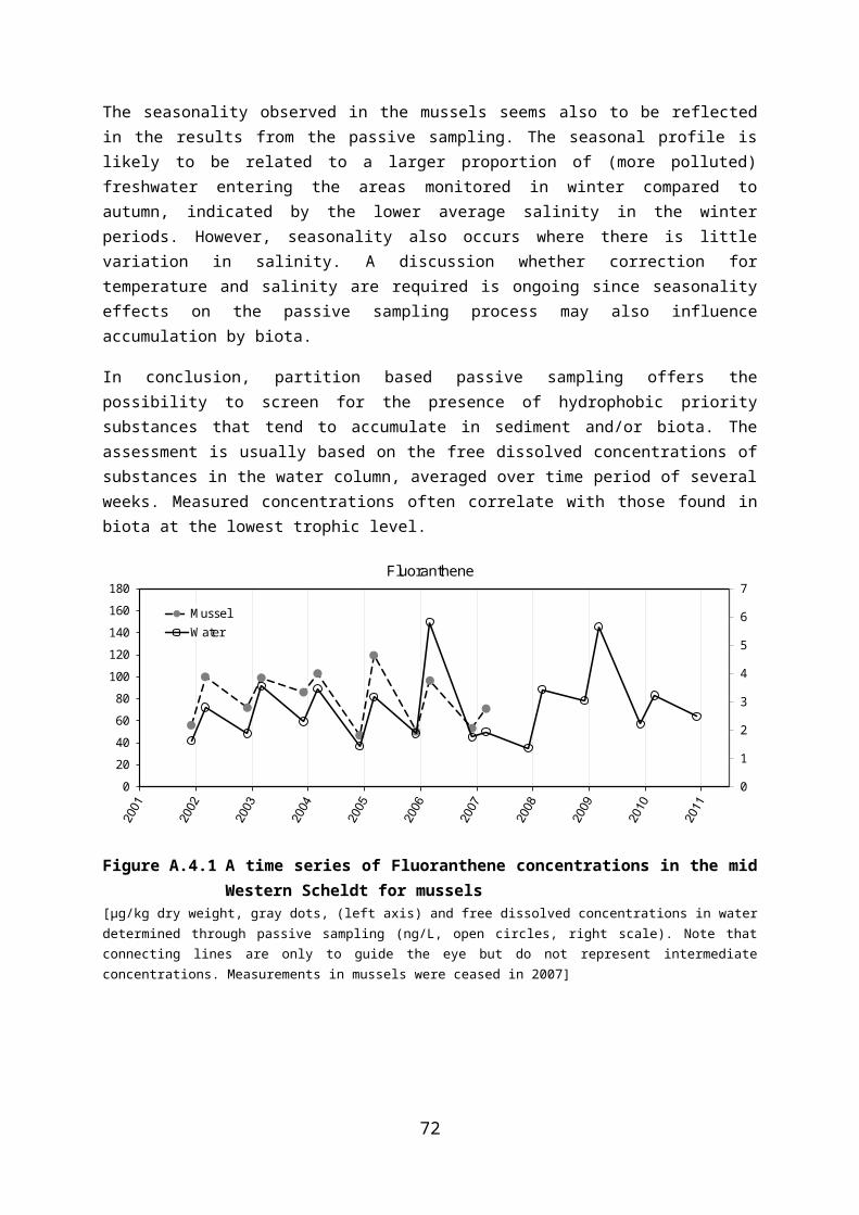
AustriaFederal Ministry of Agriculture,Forestry, Environment andWater Management

Karin Deutsch

CONCAWE Klaas den Haan

Czech RepublicMasaryk University Branislav Vrana

SpainInstituto Español de Oceanografía Lucía Viñas

Juan Bellas

European CommissionDG ENVJoint Research Centre (JRC)

Helen ClaytonGeorg HankeMarina RicciAndrea HeldBernd Gawlik

Norman Valeria Dulio

IrelandIrish EPA Simon O’Toole

73

REFERENCESAdams RG, Lohmann R, Fernandez LA, MacFarlane JK, Gschwend PM. 2007. Polyethylene

devices: Passive samplers for measuring dissolved hydrophobic organic compounds in aquatic environments. Environmental Science and Technology, 41(4), 1317–1323.

Allan IJ, Booij K, Paschke A, Vrana B, Mills GA, Greenwood R. 2009. Field performance of seven passive sampling devices for monitoring of hydrophobic substances. Environmental Science and Technology 43, 5383-5390.

Amrhein JF, Stow CA, Wible C. 1999. Whole-fish versus filet polychlorinated-biphenyl concentrations: an analysis using classification and regression tree models. Environmental Toxicology and Chemistry 18: 1871-1823.

Andral B, Stanisiere JY, Sauzade D, Damier E, Thebault H, Galgani F, Boissery P. 2004. Monitoring chemical contamination levels in the Mediterranean based on the use of mussel caging. Marine Pollution Bulletin, 49: 704-712.

Bábek O, Hilscherová K, Nehyba S, Zeman J, Famera M, Francu J, Holoubek I , Machát J, Klánová J 2008. Contamination history of suspended river sediments accumulated in oxbow lakes over the last 25 years, Morava River (Danube catchment area), Czech Republic. Journal of Soils and Sediments. 8: 165-176.

Babut M, Miege C, Roy A, Lopes C. 2010. Transferts de contaminants du sédiment au biote et construction de modèles dans une perspective de gestion. ONEMA: 47p

Babut M, Gonzalez D, Mathieu A, Pradelle S. 2013. Surveillance des substances prioritaires dans le biote - Retour d’expérience et propositions, Onema - Irstea: 38.

Belpaire C, Goemans G, Geeraerts C, Quataert P, Parmentier K. 2008. Pollution fingerprints in eels as models for the chemical status of rivers. ICES Journal of Marine Science. 65: 1483–1491.

Bervoets L, Van Campenhout K, Reynders H, Knapen D, Covaci A, Blust R. 2009. Bioaccumulation of micropollutants and biomarker responses in caged carp (Cyprinus carpio). Ecotoxicology and Environmental Safety. 72:720-728.

Besse J-P, Geffard O, Coquery M. 2012. Relevance and applicability of active biomonitoring in continental waters under the Water Framework Directive. Trends in Analytical Chemistry, 36: 113-127.

Besse J-P, Coquery M, Lopes C, Chaumot A, Budzinski H, Labadie P, Geffard O. 2013. Caged Gammarus fossarum (Crustacea) as a robust tool for the characterization of bioavailable contamination levels in continental waters: towards the determination of threshold values. Water Research. 47:650-660.

Bevelhimer MS, Beauchamp JJ, Sample BE, Southworth GR. 1997. Estimation of whole-fish contaminant concentrations from fish fillet data. ES/ER/TM-202. Oak Ridge National Laboratory, Oak Ridge, TN, USA.

Bhavsar SP, Gewurtz SB, McGoldbrick DJ, Keir MJ, Backus SM. 2010. Changes in mercury levels in Great Lakes between 1970s and 2007. Environmental Science and Technology 44: 3273-3279.

Booij K, Hofmans HE, Fischer CV, van Weerlee EM. 2003. Temperature-Dependent Uptake Rates of Nonpolar Organic Compounds by Semipermeable Membrane Devices and Low-Density Polyethylene Membranes. Environ. Sci. Technol. 37, 361–366.

Booij K, Smedes F. 2010. An improved method for estimating in situ sampling rates of nonpolar passive samplers. Environ. Sci. Technol. 44(17), 6789–94.

Boscher A, Gobert S, Guignard C, Ziebel J, L’Hoste L, Gutleb AC, Cauchie H-M, Hoffman L, Schmidt G. 2010. Chemical contaminants in fish species from rivers in the North of Luxembourg: Potential impact on the Eurasian otter (Lutra lutra). Chemosphere. 78(7): 785-792.

74

Brázová T, Hanzelová V, Miklisová D, Šalgovičová D, Turčeková L. 2012. Biomonitoring of polychlorinated biphenyls (PCBs) in heavily polluted aquatic environment in different fish species, Environmental Monitoring and Assessment. 184: 6652-6561.

Britton JR. 2007. Reference data for evaluating the growth of common riverine fishes in the UK. Journal of Applied Ichthyology: 23: 555–560.

Bruner KA, Fisher SW, Landrum PF. 1994. The Role of the zebra mussel, Dreissena polymorpha, in contaminant cycling: I. The effect of body size and lipid content on the bioconcentration of PCBs and PAHs. J Great Lakes Res 20 (4): 725-734.

Burger J, Gaines KF, Boring CS, Stephens WL, Snodgrass J, Gochfeld M. 2001. Mercury and selenium in fish from the Savannah River: species, trophic level, and locational differences. Environmental Research. 87(2): 108-118.

Caut S, Angulo E, Courchamp F. 2009. Variation in discrimination factors (Δ15N and Δ13C): The effect of diet isotopic values and applications for diet reconstruction. Journal of Applied Ecology 46 (2): 443-453.

Conti ME, Iabucci M, Cecchetti G, Alimonti A. 2008. Influence of weight on the content of trace metals in tissues of Mytilus galloprovincialis (Lamarck, 1819): a forecast model. Environmental Monitoring assessment. 141: 27-34.

Cornelissen G, Pettersen A, Broman D, Mayer P, Breedveld GD. 2008. Field testing of equilibrium passive samplers to determine freely dissolved native polycyclic aromatic hydrocarbon concentrations. Environmental Toxicology and Chemistry, 27(3), 499.

Desmet M, Mourier B, Mahler B, van Metre P, Roux G, Persat H, Lefèvre I, Peretti A, Chapron E, Simonneau A, Miège C, Babut M. 2012. Spatial and Temporal Trends in PCBs in Sediment along the Lower Rhône River, France. Science of the Total Environment. 433: 189-197.

Di Toro D M. 1991. Technical Basis For Establishing Sediment Quality Criteria For Nonionic Organic Chemicals Using Equilibrium Partitioning. Environmental Toxicology and Chemistry 10: 1541-1583.

Dörner H, Skov C, Berg S, Schulze T, Beare DJ, Van Der Velde G. 2009. Piscivory and trophic position of Anguilla anguilla in two lakes: Importance of macrozoobenthos density. Journal of Fish Biology 74 (9): 2115-2131.

Drouillard KG, Hagen H, Haffner GD. 2004. Evaluation of chloroform/methanol and dichloromethane/hexane extractable lipids as a surrogate measures of sample partition capacity for organochlorines in fish tissues. Chemosphere 55: 395-400.

Dušek L, Svobodová Z, Vykusová B, Jarkovský J, Šmíd R. 2005. Bioaccumulation of mercury in muscle tissue of fish in the Elbe River (Czech Republic): multispecies monitoring study 1991–1996. Ecotoxicology and Environmental Safety. 61(2): 256-267.

Erdogrul Ö, Covaci A, Schepens P. 2005. Levels of organochlorine pesticides, polychlorinated biphenyls and polybrominated diphenyl ethers in fish species from Kahramanmaras, Turkey. Environment International. 31(5): 703-711.

EC .2000. Directive 2000/60/EC of the European Parliament and of the Council of 23 October 2000 establishing a framework for Community action in the field of water policy. [OJ L327/1, 22.12.2000]

EC. 2006. Commission regulation No 1883/2006 of December 2006 laying down methods of sampling and analysis for the official control of levels of dioxins and dioxin-like PCBs in certain foodstuffs. Official Journal of the European Union, L 364/32. Brussels, Belgium.

EC. 2007. Council Regulation (EC) No 1100/2007 of 18 September 2007 establishing measures for the recovery of the stock of European eel. Official Journal of the European Union 22.9.2007 L 248: 17–23.

EC. 2008. Directive 2008/105/EC on Environmental Quality Standards (EQSs) in the field of water policy, amending and subsequently repealing Council Directives 82/176/EEC,

75

83/513/EEC, 84/156/EEC, 84/491/EEC, 86/280/EEC and amending Directive 2000/60/EC of the European Parliament and of the Council. [OJ L348/84, 24.12.2008]

EC. 2009. Commission directive 2009/90/EC of 31 July 2009 laying down, pursuant to Directive 2000/60/EC of the European Parliament and of the Council, technical specifications for chemical analysis and monitoring of water status. Official Journal of the European Union, L 201/36. Brussels, Belgium.

EC. 2010. Guidance Document No. 25 on Chemical Monitoring of Sediment and Biota under the Water Framework Directive. Common Implementation Strategy for the Water Framework Directive Technical Report-2010-041.

EC. 2011a. Commission regulation (EU) N° 1259/2011 of 2 December 2011 amending Regulation (EC) N° 1881/2006 as regards maximum levels for dioxins, dioxin-like PCBs and non-dioxin-like PCBs in foodstuffs. Official Journal of the European Union, L 320/18. Brussels, Belgium.

EC. 2011b. Common Implementation Strategy for the Water Framework Directive (2000/60/EC) Guidance Document No. 27 Technical Guidance For Deriving Environmental Quality Standards. European Communities.

EC. 2013. Directive 2013/39/EU of the European Parliament and of the Council of 12 August 2013 amending Directives 2000/60/EC and 2008/105/EC as regards priority substances in the field of water policy. Official Journal of the European Union, L226, 1–17. EFSA (European Food Standards Agency). 2009. Guidance Document on Risk Assessment for Birds and Mammals. Parma, Italy: European Food Safety Authority. Authority EFS.358 pp.

EFSA. 2009 (to be added)European Parliament and Council, 2010. Common Implementation Strategy for the Water

Framework Directive (2000/60/EC): Guidance Document No. 25. Guidance on Chemical Monitoring of Sediment and Biota Under the Water Framework Directive. Office for Official Publications in the European Communities (Ed.), Luxembourg.

Farkas A, Salánki J, Specziár A. 2003. Age-and size-specific patterns of heavy metals in the organs of freshwater fish Abramis brama L. populating a low-contaminated site. Water Research. 37(5): 959-964.

Fernández-Sanjuan M, Faria M, Lacorte S, Barata C. 2012. "Bioaccumulation and effects of perfluorinated compounds (PFCs) in zebra mussels (Dreissena polymorpha)." Environmental Science and Pollution Research 20(4): 2661 – 2669.

Food Safety Authority of Ireland. 2009. Legislation on Chemical Contaminants. Food Safety Authority of Ireland, Dublin, Ireland.

Gewurtz SB, Backus SM, Bhavsar SP, McGoldrick DJ, de Solla SR, Murphy EW. 2011. Contaminant biomonitoring programs in the Great Lakes region: Review of approaches and critical factors. Environmental Reviews 19: 162-184.

Giltrap M, Macken A, Davoren M, McGovern E, Foley B, Larsen M, White J, McHugh B. 2012. Utilising caging techniques to investigate metal assimilation in Nucella lapillus, Mytilus edulis and Crassostrea gigas at three Irish coastal locations. Estuarine, Coastal and Shelf Science In press

Gobas FAPC, Wilcockson JB, Russell RW. Haffner GD. 1999. Mechanism of biomagnification in fish under laboratory and field conditions. Environmental Science and Technology 33: 133-141.

Goeritz I, Falk S, Stahl T, Schäfers, Schlechtriem C. 2013. Biomagnification and tissue distribution of perfluoroalkyl substances in market-size rainbow trout (Oncorhynchus mykiss). Environmental Toxicology and Chemistry 32(9): 2078-2088.

Goldstein RM, Brigham ME, Stauffer JC. 1996. Comparison of mercury concentrations in liver, muscle, whole bodies, and composites of fish from the Red River of the North. Canadian Journal of Fisheries and Aquatic Sciences 53: 244-252.

76

Gust M, Buronfosse T, Geffard O, Mons R, Queau H, Mouthon J, Garric J. 2010. In situ biomonitoring of freshwater quality using the New Zealand mudsnail Potamopyrgus antipodarum (Gray) exposed to waste water treatment plant (WWTP) effluent discharges. Water Research. 44: 4517-4528.

Gust M, Buronfosse T, Geffard O, Coquery M, Mons R, Abbaci K, Giamberini L, Garric J. 2011. Comprehensive biological effects of a complex field poly-metallic pollution gradient on the New Zealand mudsnail Potamopyrgus antipodarum (Gray). Aquatic Toxicology. 101: 100-108.

Hannah R.W, Rankin PS, Blume MTO. 2012. Use of novel cage system to measure postrecompression survival of Northeast Pacific Rockfish. Marine and Coastal Fisheries: Dynamics and Ecosystem Science. 4: 46-56.

Hajšlová J, Pulkrabová J, Poustka J, Čajka T, Randák T. 2007. Brominated flame retardants and related chlorinated persistent organic pollutants in fish from river Elbe and its main tributary Vltava. Chemosphere. 69(8), 1195-1203.

Harman C, Allan IJ, Vermeirssen ELM. 2012. Calibration and use of the polar organic chemical integrative sampler--a critical review. Environmental Toxicology and Chemistry, 31(12), 2724–38.

Heber GE, Keenleyside KA. 1995. To normalize or not to normalize? Fat is the question. Environmental Toxicology and Chemistry 14(5): 801-807.

Herve S, Heinonen P, Paasivirta J. 2002. Survey of organochlorines in Finnish watercourses by caged mussel method. Resources, Conservation and Recycling. 35: 105-115.

HELCOM 2013. Manual for monitoring in the COMBINE programme of HELCOM. Available at:

http://www.helcom.fi/action-areas/monitoring-and-assessment/manuals-and-guidelines/combine-manual accessed 13 December 2013.

Huckins JN, Petty JD, Booij K. 2006. Monitors of Organic Chemicals in the Environment: Semipermeable Membrane Devices (p. 222). New York, USA: Springer.

ICES. 2009. Report of the Joint ICES/OSPAR Study Group on Integrated Monitoring of Contaminants and Biological Effects (SGIMC), 12–15 January 2009, Copenhagen, Denmark. ICES CM 2008/ACOM:30. 64 pp. http://www.ices.dk/reports/ACOM/2009/SGIMC/sgimc_2009.pdf.

ISO (International Organisation for Standardisation). 2008. Water quality - Sampling: Part 20: Guidance on the use of sampling data for decision making -Compliance with thresholds and classification. International Organization for Standardization. ISO 5667-20:2008(E). Switzerland.

ISO. (International Organisation for Standardisation). 2011. Water quality - sampling - Part 23: Guidance on passive sampling in surface waters International Organization for Standardization. ISO 5667-23:2011. Switzerland.

Jurgens M, Johnson A, Jones K, Hughes D and Lawlor A. 2013. The presence of EU priority substances mercury, hexachlorobenzene, hexachlorobutadiene and PBDEs in wild fish from four English rivers. Science of the Total Environment 461-462, 441-452.

Kopp D, Cucherousset J, Syväranta J, Martino A, Céréghino R, Santoul F. 2009. Trophic ecology of the pikeperch (Sander lucioperca) in its introduced areas: a stable isotope approach in southwestern France. Comptes Rendus - Biologies 332 (8): 741-746.

Lacaze E, Devaux A, Mons R, Bony S, Garric J, Geffard A, Geffard O. 2011. DNA damage in caged Gammarus fossarum amphipods: a tool for freshwater genotoxicity assessment. Environmental Pollution. 159: 1682-1691.

Law RJ, Barry J, Barber LJ, Bersuder P, Deaville R, Reid RJ, Brownlow A, Penrose R, Barnett J, Loveridge J, Smith B, Jepson PD. 2012. Contaminants in cetaceans from UK waters: status as assessed within the Cetacean Strandings Investigation Programme from 1990 to 2008. Marine Pollution Bulletin. 64: 1485-1494.

77

http://www.ices.dk/reports/ACOM/2009/SGIMC/sgimc_2009.pdf

http://www.helcom.fi/action-areas/monitoring-and-assessment/manuals-and-guidelines/combine-manual%20accessed%2013%20December%202013

http://www.helcom.fi/action-areas/monitoring-and-assessment/manuals-and-guidelines/combine-manual%20accessed%2013%20December%202013

Lazzara R, Fernandes D, Faria M, López JF, Tauler R, Porte C. 2012. Changes in lipid content and fatty acid composition along the reproductive cycle of the freshwater mussel Dreissena polymorpha: Its modulation by clofibrate exposure. Sci Total Environ 432: 195-201.

Lohmann R, Booij K, Smedes F, Vrana B. 2012. Use of passive sampling devices for monitoring and compliance checking of POP concentrations in water. Environmental Science and Pollution Research International, 19(6), 1885–95.

Lopes C, Persat H, Babut M. 2012. Transfer of PCBs from bottom sediment to freshwater river fish species: a food-web modelling approach in the Rhône River (France) in support of sediment management. Ecotoxicology and Environmental Safety. 81: 17-26.

MacGregor K, Oliver IW, Duguid A, Ridgway IM. 2011. Persistent Organic Pollutants in Scottish Freshwater Biota Monitoring options, current levels and the way forward. Scottish Environmental Protection Agency.

Macgregor K, Oliver IW, Harris L, Ridgway IM. 2010. Persistent organic pollutants (PCB, DDT, HCH, HCB & BDE) in eels (Anguilla anguilla) in Scotland: Current levels and temporal trends. Environ. Pollut. 158: 2402-2411

Madenjian CP. 2011. Sex effect on polychlorinated biphenyl concentrations in fish: a synthesis. Fish and Fisheries. 12(4): 451-460.

Maes J, Belpaire C, Goemans G. 2008. Spatial variations and temporal trends between 1994 and 2005 in polychlorinated biphenyls, organochlorine pesticides and heavy metals in European eel (Anguilla anguilla L.) in Flanders, Belgium. Environmental Pollution. 153: 223-237.

Manirakiza P, Covaci A, Schepens P. 2001. Comparative Study on Total Lipid Determination using Soxhlet, Roese-Gottlieb, Bligh and Dyer, and Modified Bligh and Dyer Extraction Methods. Journal of Food Composition and Analysis: 14: 93-100.

Marigomez I, Zorita I, Izagirre U, Ortiz-Zarragoitia M, Navarro P, Etxebarria N, Orbea A, Soto M, Cajaraville MP. 2013. Combined use of native and caged mussels to assess biological effects of pollution through the integrative biomarker approach. Aquatic Toxicology. 136-137: 32-48.

Martin JW, Mabury SA, Solomon KR, Muir DCG. 2003. Bioconcentration and tissue distribution of perfluorinated acids in rainbow trout (Oncorhynchus mykiss). Environmental Toxicology and Chemistry. 22(1): 196-204.

Mayer P, Tolls J, Hermens L, Mackay D. 2003. Equilibrium Sampling Devices. Environmental Science and Technology, 37(9), 184A–191A.

McIntyre JK, Beauchamp DA. 2007. Age and trophic position dominate bioaccumulation of mercury and organochlorines in the food web of Lake Washington. Science of the Total Environment. 372(2): 571-584.

Moermond CTA, Verbruggen EMJ. 2013. An evaluation of bioaccumulation data for hexachlorobenzene to derive water quality standards according to the EU-WFD methodology. Integrated Environmental Assessment and Management 9 (1): 87-97.

Mourier B, Desmet M, Van Metre PC, Mahler BJ, Perrodin Y, Roux G, Bedell J-P, Lefèvre I, Babut M. 2014. Historical records, sources, and spatial trends of PCBs along the Rhône River (France). Science of the Total Environment. 476-477: 568-576.

Nfon E, Cousins IT, Broman D. 2008. Biomagnification of organic pollutants in benthic and pelagic marine food chains from the Baltic Sea. Sci Total Environ 397 (1-3): 190-204.

Noël L, Chekri R, Millour S, Merlo M, Leblanc JC, Guérin T. 2013. Distribution and relationships of As, Cd, Pb and Hg in freshwater fish from five French fishing areas. Chemosphere 90: 1900-1910.

Nyberg E, Faxneld S, Danielsson S, Bignert A. 2013. The National Swedish Contaminant Monitoring Programme for Freshwater Biota, 2012. Report Nr. 13:2012 for the Swedish EPA by the Department of Environmental Research and Monitoring at the Swedish Museum of Natural History, 214 pp.

78

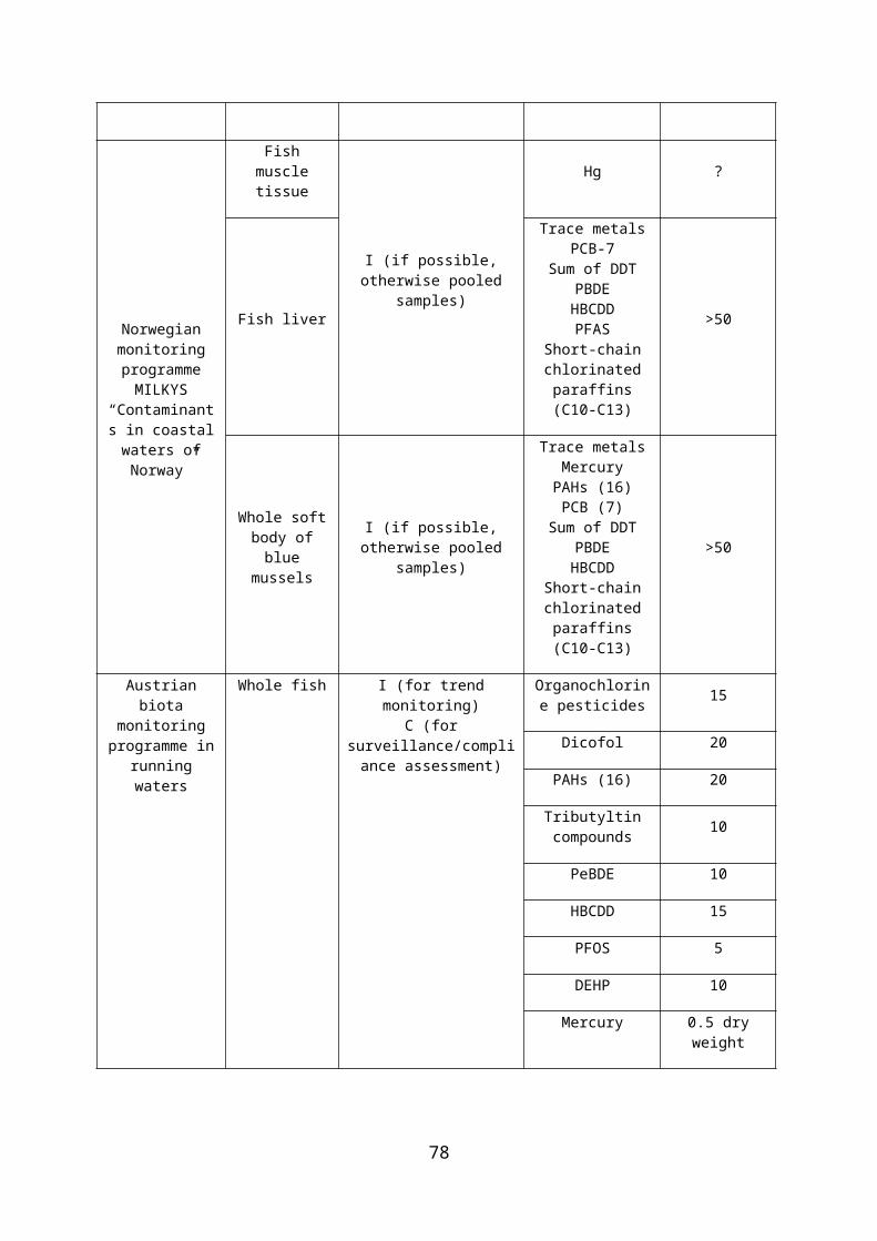
OSPAR. 2009. JAMP guidelines for monitoring contaminants in biota. Ref No 1999-2, OSPAR Commission, London.

Peterson SA, Van Sickle J, Hughes RM, Schacher JA, Echols SF. 2005. A biopsy procedure for determining filet and predicting whole-fish mercury concentration. Archives of Environmental Contamination and Toxicology 48: 99-107.

Pleissner D, Eriksen NT, Lundgreen K, Riisgård HU. 2012. Biomass composition of blue mussels, Mytilus edulis, is affected by living site and species of ingested microalgae. ISRN Zoology 2012: 1-12.

Post DM. 2002. Using stable isotopes to estimate trophic position: Models, methods, and assumptions. Ecology 83 (3): 703-718.

Pulkrabová J, Hajšlová J, Poustka J, Kazda R. 2007. Fish as biomonitors of polybrominated diphenyl ethers and hexabromocyclododecane in Czech aquatic ecosystems: pollution of the Elbe River Basin. Environmental Health Perspectives. 115(S-1): 28.

R Development Core Team. 2010. R: a language and environment for statistical computing. R Foundation for Statistical Computing, Vienna, Austria. ISBN 3-900051-07-0, url http://www.R-project.org/

Reichenberg F, Mayer P. 2006. Two complementary sides of bioavailability: accessibility and chemical activity of organic contaminants in sediments and soils. Environmental Toxicology and Chemistry / SETAC, 25(5), 1239–45.

Roosens L, Dirtu AC, Goemans G, Belpaire C, Gheorghe A, Neels H, Blust R, Covaci A. 2008. Brominated flame retardants and polychlorinated biphenyls in fish from the river Scheldt, Belgium. Environment International. 34: 976–983.

Rusina TP, Smedes F, Koblizkova M, Klanova J. 2010. Calibration of silicone rubber passive samplers: experimental and modelled relations between sampling rate and compound properties. Environmental Science & Technology, 44(1), 362–7.

Sharma CM, Rosseland BO, Almvik M, Eklo OM. 2009. Bioaccumulation of organochlorine pollutants in the fish community in Lake Årungen, Norway. Environmental Pollution. 157(8): 2452-2458.

Smedes F. 2007. Monitoring of chlorinated biphenyls and polycyclic aromatic hydrocarbons by passive sampling in concert with deployed mussels. In R. Greenwood, G. Mills, and B. Vrana (Eds.), Comprehensive Analytical Chemistry 48; Passive sampling techniques in Environmental Monitoring (pp. 407–448). Amsterdam: Elsevier.

Smedes F, Booij K. 2012. Guidelines for passive sampling of hydrophobic contaminants in water using silicone rubber samplers. ICES TECHNIQUES IN MARINE E ENVIRONMENTAL SCIENCES, 52.

Smedes F, Geertsma RW, Van Der Zande T, Booij K. 2009. Polymer-water partition coefficients of hydrophobic compounds for passive sampling: Application of cosolvent models for validation. Environmental Science and Technology, 43(18), 7047–7054.

Smedes F, Zande T, Van Der Tixier C, Davies IM. 2007. ICES Passive sampling trial survey for water and sediment (PSTS) 2006 – 2007. Part 2: Laboratory inter-comparison, analytical issues and lessons learned. Retrieved from http://info.ices.dk/products/AnnualRep/ASCproceedings/2007/Annual Science Conference 2007/CM-2007/J/J0307.pdf

Smedes F, van Vliet LA, Booij K. 2013. Multi-Ratio Equilibrium Passive Sampling Method to Estimate Accessible and Pore Water Concentrations of Polycyclic Aromatic Hydrocarbons and Polychlorinated Biphenyls in Sediment. Environ. Sci. Technol. 47, 510–517.

Smit CE. 2005. Energy and moisture content and assimilation efficiency of bird and mammal food. Bilthoven, The Netherlands: National Institute for Public Health and the Environment (RIVM). Report nr. RIVM report 601516013/2005. 57-71 pp.

79

http://info.ices.dk/products/AnnualRep/ASCproceedings/2007/Annual%20Science%20Conference%202007/CM-2007/J/J0307.pdf

http://info.ices.dk/products/AnnualRep/ASCproceedings/2007/Annual%20Science%20Conference%202007/CM-2007/J/J0307.pdf

Stapleton HM, Baker JE. 2003. Comparing polybrominated diphenyl ether and polychlorinated biphenyl bioaccumulation in a food web in Grand Traverse Bay, Lake Michigan. Archives of environmental contamination and toxicology 45(2): 227-234.

Stien X, Percic P, Gnassia-Barelli M, Roméo M, Lafaurie M. 1998. Evaluation of biomarkers in caged fishes and mussels to assess the quality of waters in a bay of the NW Mediterranean Sea. Environmental Pollution. 99: 339-345.

Takeuchi I, Miyoshi N, Mizukawa K, Takada H, Ikemoto T, Omori K, Tsuchiya K. 2009. Biomagnification profiles of polycyclic aromatic hydrocarbons, alkylphenols and polychlorinated biphenyls in Tokyo Bay elucidated by δ13C and δ15N isotope ratios as guides to trophic web structure. Marine Pollution Bulletin 58 (5): 663-671.

Turja R, Soirinsuo A, Budzinski H, Devier M-H, Lehtonen KK. 2013. Biomarker responses and accumulation of hazardous substances in mussels (Mytilus trossulus) transplanted along a pollution gradient close to an oil terminal in the Gulf of Finland (Baltic Sea). Comparative Biochemistry and Physiology, Part C 157: 80-92.

Uhl M, Offenthaler I, Hartl W, et al. 2010. Monitoring von Schadstoffen in biota. Pilotstudie 2010. Bundesministerium für Land- und Forstwirtschaft, Umwelt und Wasserwirtschaft report. Vienna, Austria.

Vander Zanden MJ, Cabana G, Rasmussen JB. 1997. Comparing trophic position of freshwater fish calculated using stable nitrogen isotope ratios (δ15N) and literature dietary data. Canadian Journal of Fisheries and Aquatic Sciences 54 (5): 1142-1158.

Van Metre PC, Mahler BJ. 2005. "Trends in hydrophobic organic contaminants in urban and reference lake sediments across the United States, 1970-2001." Environmental Science and Technology. 39(15): 5567-5574.

Wan Y, Jin X, Hu J, Jin F. 2007. Trophic dilution of polycyclic aromatic hydrocarbons (PAHs) in a marine food web from Bohai Bay, North China. Environ Sci Technol 41 (9): 3109-3114.

Williams LL, Giesy JP, DeGalan N, Verbrugge DA, Tillitt DE, Ankley GT, Welch RL. 1992. Prediction of concentrations of 2,3,7,8-tetrachlorodibenzo-p-dioxin equivalents from total concentrations of polychlorinated biphenyls in fish fillets. Environmental Science and Technology. 26: 1151-1159.

Wood SN. 2006. Generalized Additive Models: an introduction with R. Chapman and Hall/CRC, London. 410 pp. ISBN 1-584884-74-6.

80

circabc.europa.eu · web viewenvironmental quality standard. a term most often used in reference to...

Documents