Aggregate Operations Planning

Class-1 , 2 and 3

Wish you all a very happy new year 2013 and welcome to Operations management-II

Group Structure for OM-IIGrp No. SR. NO. NAME

12PGDM-BHU001 Aastha Bansal12PGDM-BHU005 Anant Ashesh12PGDM-BHU009 Iliyas Ahmad12PGDM-BHU013 Jillam Parida12PGDM-BHU002 Aditya Anshuman Dash12PGDM-BHU006 Apurv Chaturvedi12PGDM-BHU010 Ishaan Rattanpal12PGDM-BHU014 Jubin Joseph 12PGDM-BHU003 Ajay Pratap Singh 12PGDM-BHU007 Bibhu Prasad Rath12PGDM-BHU011 Irshad Alam12PGDM-BHU015 Kunder Dhiraj Sadhu12PGDM-BHU004 Ajeet Singh Chauhan12PGDM-BHU008 Dipanjan Bhattachrya12PGDM-BHU012 Japkirat Singh Oberai12PGDM-BHU016 Lovepreet Singh12PGDM-BHU017 Megha Kulbhushan12PGDM-BHU022 Suman Sekhar Pradhan12PGDM-BHU023 Sujeet Singh12PGDM-BHU020 Siladitya Sahoo12PGDM-BHU021 Singamsetti Subba Rao12PGDM-BHU018 Shiva Krishna Padhi12PGDM-BHU019 Shivani Parashar12PGDM-BHU025 Yashraj Behera

I

II

VI

III

IV

V

Aggregate Planning

• Overview of Sales and Operations Planning Activities,

• The Aggregate Operations Plan,• Aggregate Planning Techniques• Production-Planning Hierarchy• Aggregate Planning• Master Production Scheduling• Types of Production-Planning and

Control Systems

Aggregate Planning

Attempts to match the supply of and demand for a product or service by determining the appropriate quantities and timing of inputs, transformation, and outputs. Decisions made on production, staffing, inventory and backorder levels.

Operations Planning Overview

• Long-range planning– Greater than one year planning horizon– Usually with yearly increments

• Intermediate-range planning– Six to eighteen months – Usually with monthly or quarterly increments

• Short-range planning– One day to less than six months– Usually with weekly increments

Hierarchical Production PlanningForecasts neededDecision ProcessDecision Level

Annual demand byitem and by region

Allocatesproduction

among plantsCorporate

Monthly demandfor 15 months by

product type

Determinesseasonal plan by

product type

Plant manager

Monthly demandfor 5 months by

item

Determines monthlyitem production

schedules

Shopsuperintendent

Production Planning Hierarchy

Master Production Scheduling Master Production Scheduling

Production Planning and Control SystemsProduction Planning and Control Systems

Pond DrainingPond DrainingSystemsSystems

Aggregate Operations PlanningAggregate Operations Planning

PushPushSystems Systems

PullPullSystemsSystems

Focusing onFocusing onBottlenecksBottlenecks

Long-Range Capacity PlanningLong-Range Capacity Planning

Production Planning HorizonsProduction Planning HorizonsProduction Planning HorizonsProduction Planning Horizons

Master Production Scheduling Master Production Scheduling

Production Planning and Control SystemsProduction Planning and Control Systems

Pond DrainingPond DrainingSystemsSystems

Aggregate Operations PlanningAggregate Operations Planning

PushPushSystems Systems

PullPullSystemsSystems

Focusing onFocusing onBottlenecksBottlenecks

Long-Range Capacity PlanningLong-Range Capacity PlanningLong-RangeLong-Range

(years)(years)

Medium-RangeMedium-Range(6-18 months)(6-18 months)

Short-RangeShort-Range(weeks)(weeks)

Very-Short-RangeVery-Short-Range(hours - days)(hours - days)

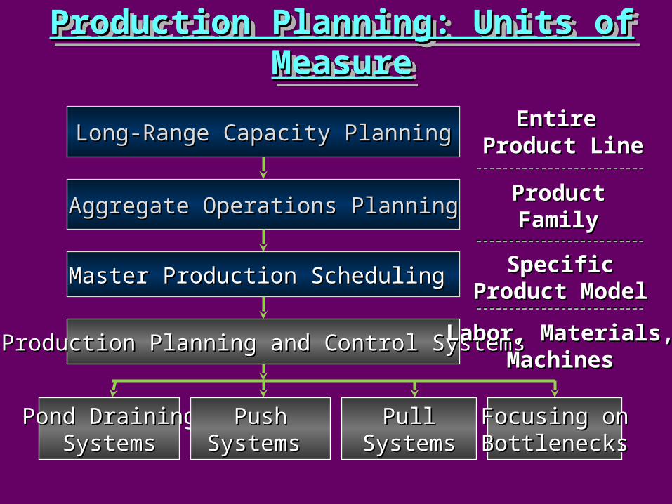
Production Planning: Units of MeasureProduction Planning: Units of MeasureProduction Planning: Units of MeasureProduction Planning: Units of Measure

Master Production SchedulingMaster Production Scheduling

Production Planning and Control SystemsProduction Planning and Control Systems

Pond DrainingPond DrainingSystemsSystems

Aggregate Operations PlanningAggregate Operations Planning

PushPushSystems Systems

PullPullSystemsSystems

Focusing onFocusing onBottlenecksBottlenecks

Long-Range Capacity PlanningLong-Range Capacity PlanningEntire Entire

Product LineProduct Line

ProductProductFamilyFamily

SpecificSpecificProduct ModelProduct Model

Labor, Materials,Labor, Materials,MachinesMachines

Why Aggregate Planning Is Necessary

• Fully load facilities and minimize overloading and under loading

• Make sure enough capacity available to satisfy expected demand

• Plan for the orderly and systematic change of production capacity to meet the peaks and valleys of expected customer demand

• Get the most output for the amount of resources available

Aggregate Planning

• Goal: Specify the optimal combination of– production rate (units completed per unit of time)– workforce level (number of workers)– inventory on hand (inventory carried from

previous period)

Required Inputs to the Aggregate Planning System

Planning for

production

External capacity

Competitors’behavior

Raw material availability

Market demand

Economic conditions

Currentphysical capacity

Current workforce

Inventory levels

Activities required for production

Internal to firm

External to firm

Outputs

• A production plan: aggregate decisions for each period in the planning horizon about– workforce level– inventory level– production rate

• Projected costs if the production plan was implemented

Medium-Term Capacity Adjustments

• Workforce level– Hire or layoff full-time workers– Hire or layoff part-time workers– Hire or layoff contract workers

• Utilization of the work force– Overtime– Idle time (undertime) – Reduce hours worked

• . . . more

Medium-Term Capacity Adjustments

• Inventory level– Finished goods inventory– Backorders/lost sales

• Subcontract

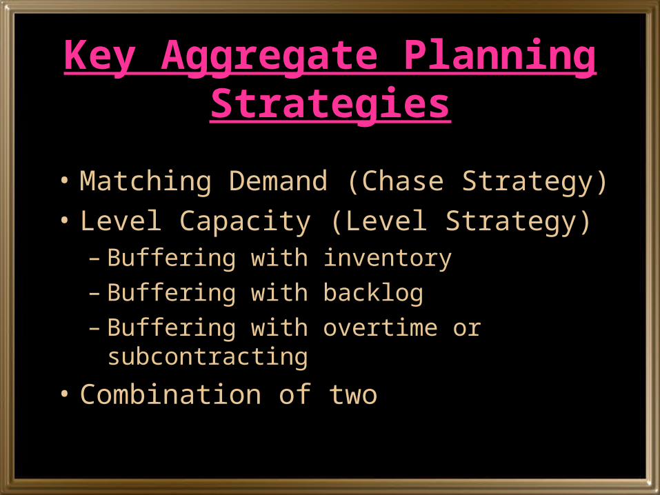
Key Aggregate Planning Strategies

• Matching Demand (Chase Strategy)

• Level Capacity (Level Strategy)– Buffering with inventory– Buffering with backlog– Buffering with overtime or subcontracting

• Combination of two

Matching Demand Strategy

• Capacity (Production) in each time period is varied to exactly match the forecasted aggregate demand in that time period

• Capacity is varied by changing the workforce level

• Finished-goods inventories are minimal

• Labor and materials costs tend to be high due to the frequent changes

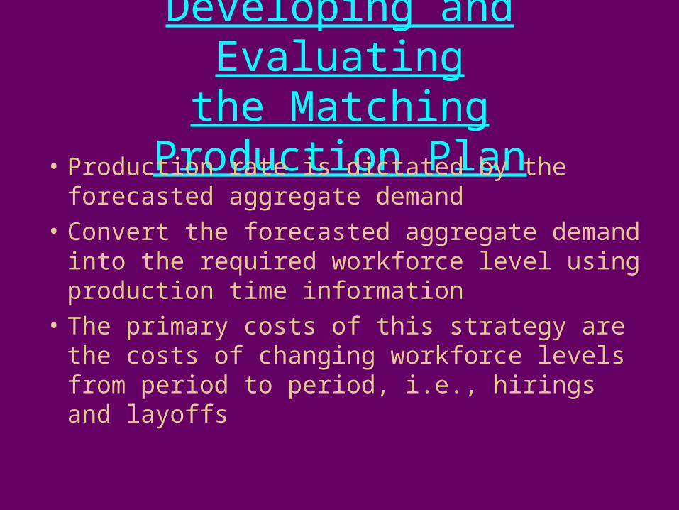
Developing and Evaluatingthe Matching Production Plan

• Production rate is dictated by the forecasted aggregate demand

• Convert the forecasted aggregate demand into the required workforce level using production time information

• The primary costs of this strategy are the costs of changing workforce levels from period to period, i.e., hirings and layoffs

Level Capacity Strategy

• Capacity (production rate) is held level (constant) over the planning horizon

• The difference between the constant production rate and the demand rate is made up (buffered) by inventory, backlog, overtime, part-time labor and/or subcontracting

Developing and Evaluatingthe Level Production Plan

• Assume that the amount produced each period is constant, no hirings or layoffs

• The gap between the amount planned to be produced and the forecasted demand is filled with either inventory or backorders, i.e., no overtime, no idle time, no subcontracting

• . . . more

Balancing Aggregate Demandand Aggregate Production Capacity

0

2000

4000

6000

8000

10000

Jan Feb Mar Apr May Jun

45005500

7000

10000

8000

6000

0

2000

4000

6000

8000

10000

Jan Feb Mar Apr May Jun

4500 4000

90008000

4000

6000

Suppose the figure to the right represents forecast demand in units.

Now suppose this lower figure represents the aggregate capacity of the company to meet demand.

What we want to do is balance out the production rate, workforce levels, and inventory to make these figures match up.

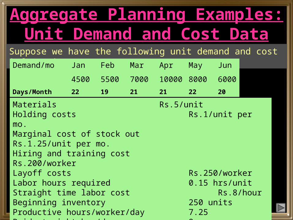
Aggregate Planning Examples: Unit Demand and Cost Data

Materials Rs.5/unitHolding costs Rs.1/unit per mo.Marginal cost of stock out Rs.1.25/unit per mo.Hiring and training cost Rs.200/workerLayoff costs Rs.250/workerLabor hours required 0.15 hrs/unitStraight time labor cost Rs.8/hourBeginning inventory 250 unitsProductive hours/worker/day 7.25Paid straight hrs/day 8Present Workforce strength 7

Suppose we have the following unit demand and cost information:

Demand/mo Jan Feb Mar Apr May Jun

4500 5500 7000 10000 8000 6000

Days/Month 22 19 21 21 22 20

Determining Straight Labor Costs and Output

Jan Feb Mar Apr May JunDays/mo 22 19 21 21 22 20Hrs/worker/mo 159.5 137.75 152.25 152.25 159.5 145Units/worker 1063.3

3918.33 1015 1015 1063.33 966.67

Rs./worker 1,408 1,216 1,344 1,344 1,408 1,280

Productive hours/worker/day 7.25Paid straight hrs/day 8

Demand/mo Jan Feb Mar Apr May Jun

4500 5500 7000 10000 8000 6000

Given the demand and cost information below, what are the aggregate hours/worker/month, units/worker, and dollars/worker?

7.25x22

(7.25 x 22) / 0.15=1063.3322x8hrsxRs.8=Rs.1408

Chase Strategy(Hiring & Firing to meet demand)

JanDays/mo 22Hrs/worker/mo 159.5Units/worker 1,063.33Rs./worker Rs.1,408

JanDemand 4,500Beg. inv. 250Net req. 4,250Req. workers 3.997HiredFired 3Workforce 4

Ending inventory 0

Lets assume our current workforce is 7 workers.

First, calculate net requirements for production, or 4500-250=4250 units

Then, calculate number of workers needed to produce the net requirements, or 4250/1063.33=3.997 or 4 workers

Finally, determine the number of workers to hire/fire. In this case we only need 4 workers, we have 7, so 3 can be fired.

Jan Feb Mar Apr May JunDays/mo 22 19 21 21 22 20Hrs/worker/mo 159.5 137.75 152.25 152.25 159.5 145Units/worker 1,063 918 1,015 1,015 1,063 967Rs./worker Rs.1,408 1,216 1,344 1,344 1,408 1,280

Jan Feb Mar Apr May JunDemand 4,500 5,500 7,000 10,000 8,000 6,000Beg. inv. 250Net req. 4,250 5,500 7,000 10,000 8,000 6,000Req. workers 3.997 5.989 6.897 9.852 7.524 6.207Hired 2 1 3Fired 3 2 1Workforce 4 6 7 10 8 7

Ending inventory 0 0 0 0 0 0

Below are the complete calculations for the remaining months in the six month planning horizon.

Jan Feb Mar Apr May Jun

Demand 4,500 5,500 7,000 10,000 8,000 6,000

Beg. inv. 250

Net req. 4,250 5,500 7,000 10,000 8,000 6,000

Req. workers 3.997 5.989 6.897 9.852 7.524 6.207

Hired 2 1 3

Fired 3 2 1

Workforce 4 6 7 10 8 7

Ending inventory 0 0 0 0 0 0

Jan Feb Mar Apr May Jun Costs

Material(Rs.) 21,250.00 27,500.00 35,000.00 50,000.00 40,000.00 30,000.00 203,750.00

Labor 5632 7,296 9408 13,440 11264 8960 56,000.00

Hiring cost 400.00 200.00 600.00 1,200.00

Firing cost 750.00 500.00 250.00 1,500.00

262,450.00

Below are the complete calculations for the remaining months in the six month planning horizon with the other costs included.

Rs.

Level Workforce Strategy (Surplus and Shortage Allowed)

JanDemand 4,500Beg. inv. 250Net req. 4,250Workers 6Production 6,380Ending inventory 2,130Surplus 2,130Shortage

Lets take the same problem as before but this time use the Level Workforce strategy.

This time we will seek to use a workforce level of 6 workers.

Jan Feb Mar Apr May JunDemand 4,500 5,500 7,000 10,000 8,000 6,000Beg. inv. 250 2,130 2,140 1,230 -2,680 -4,300Net req. 4,250 3,370 4,860 8,770 10,680 10,300Workers 6 6 6 6 6 6Production 6,380 5,510 6,090 6,090 6,380 5,800Ending inventory 2,130 2,140 1,230 -2,680 -4,300 -4,500Surplus 2,130 2,140 1,230Shortage 2,680 4,300 4,500

Below are the complete calculations for the remaining months in the six month planning horizon.

Assumption: Shortage of a month can be made off during the next month.

Jan Feb Mar Apr May Jun4,500 5,500 7,000 10,000 8,000 6,000

250 2,130 10 1230 -2680 -4,3004,250 3,370 4,860 8,770 10,680 10,300

6 6 6 6 6 66,380 5,510 6,090 6,090 6,380 5,8002,130 2,140 1,230 -2,680 -4,300 -4,5002,130 2,140 1,230

2,680 4,300 4,500

Jan Feb Mar Apr May Jun8,448 7,296 8,064 8,064 8,448 7,68031,900 27,550 30,450 30,450 31,900 29,000 181,250.002,130 2,140 1,230

3,350 5,375 5,625

Below are the complete calculations for the remaining months in the six month planning horizon with the other costs included

Below are the complete calculations for the remaining months in the six month planning horizon with the other costs included

Note, total costs under this strategy are less than Chase at Rs. 262,450/-

Note, total costs under this strategy are less than Chase at Rs. 262,450/-

LaborMaterialStorageStockout

5,500.00

48,000.00

14,350.00

249,100.00Rs.

Aggregate Plans for Services• For standardized services, aggregate planning

may be simpler than in systems that produce products

• For customized services,– there may be difficulty in specifying the nature

and extent of services to be performed for each customer

– customer may be an integral part of the production system

• Absence of finished-goods inventories as a buffer between system capacity and customer demand

Preemptive Tactics

• There may be ways to manage the extremes of demand:– Discount prices during the valleys.... have

a sale– Peak-load pricing during the highs ....

electric utilities

Yield Management

It is the process of allocating the right type of capacity to right type of customer at the right price and time to maximize the revenue.

Yield Management

It is most effective under following situation.

• Demand can be segmented.

• Fixed cost is high and variable

cost is low.

• Inventory is perishable.

• Product can be sold in advance

• Demand is highly variable

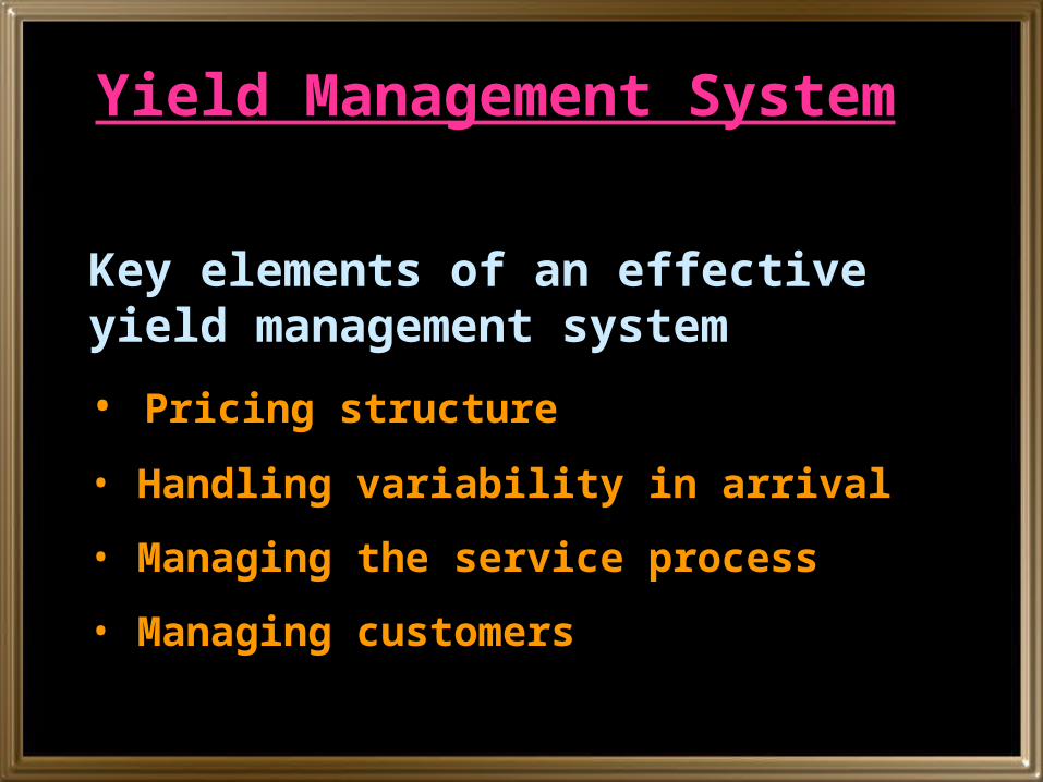
Yield Management System

Key elements of an effective yield management system

• Pricing structure

• Handling variability in arrival

• Managing the service process

• Managing customers

Master Production Scheduling (MPS)

Objectives of MPS• Determine the quantity and timing of

completion of end items over a short-range planning horizon.

• Schedule end items (finished goods and parts shipped as end items) to be completed promptly and when promised to the customer.

• Avoid overloading or underloading the production facility so that production capacity is efficiently utilized and low production costs result.

The rules for schedulingThe rules for scheduling

No ChangeNo Change+/- 5%+/- 5%

ChangeChange

+/- 10%+/- 10%

ChangeChange

+/- 20%+/- 20%

ChangeChange

+/- 20%+/- 20%

ChangeChangeFrozenFrozen

FirmFirm

FullFullOpenOpen

1-21-2 weeksweeks

2-42-4weeksweeks

4-64-6weeksweeks

6+ 6+ weeksweeks

Time Fences

Time Fences• The rules for scheduling:

– Do not change orders in the frozen zone– Do not exceed the agreed on percentage

changes when modifying orders in the other zones

– Try to level load as much as possible– Do not exceed the capacity of the system

when promising orders.– If an order must be pulled into level load, pull

it into the earliest possible week without missing the promise.

Developing an MPS• Using input information

– Customer orders (end items quantity, due dates)

– Forecasts (end items quantity, due dates)– Inventory status (balances, planned receipts)– Production capacity (output rates, planned

downtime)

• Schedulers place orders in the earliest available open slot of the MPS

• . . . more

Developing an MPS

• Schedulers must:– estimate the total demand for products

from all sources– assign orders to production slots– make delivery promises to customers, and– make the detailed calculations for the MPS

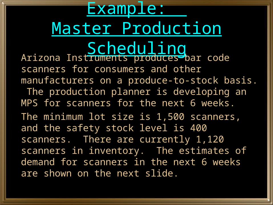
Example: Master Production Scheduling

Arizona Instruments produces bar code scanners for consumers and other manufacturers on a produce-to-stock basis. The production planner is developing an MPS for scanners for the next 6 weeks.

The minimum lot size is 1,500 scanners, and the safety stock level is 400 scanners. There are currently 1,120 scanners in inventory. The estimates of demand for scanners in the next 6 weeks are shown on the next slide.

• Demand Estimates

CUSTOMERS CUSTOMERS

BRANCH WAREHOUSES BRANCH WAREHOUSES

MARKET RESEARCH MARKET RESEARCH

PRODUCTION RESEARCHPRODUCTION RESEARCH

500500

200200

00

1010

11

00

5050

300300

10001000

00

00

500500

400400

22 33 44

200200

000000

300300500500

00101000

700700

6655

10001000

200200

WEEKWEEK

Example: Master Production Scheduling

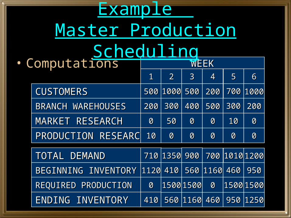
• Computations

CUSTOMERS CUSTOMERS

BRANCH WAREHOUSES BRANCH WAREHOUSES

MARKET RESEARCH MARKET RESEARCH

PRODUCTION RESEARCHPRODUCTION RESEARCH

500500

200200

00

1010

11

00

5050

300300

10001000

00

00

500500

400400

22 33 44

200200

000000

300300500500

00101000

700700

6655

10001000

200200

WEEKWEEK

TOTAL DEMAND TOTAL DEMAND

BEGINNING INVENTORY BEGINNING INVENTORY

REQUIRED PRODUCTIONREQUIRED PRODUCTION

ENDING INVENTORYENDING INVENTORY

710710

11201120

00

410410 560560

15001500

410410

13501350

11601160

15001500

900900

560560

700700

12501250950950460460

46046011601160

150015001500150000

10101010 12001200

950950

Example Master Production Scheduling

• MPS for Bar Code Scanners

SCANNER PRODUCTIONSCANNER PRODUCTION 00 15001500 15001500 150015001500150000

11 22 33 44 6655

WEEKWEEK

Example Master Production Scheduling

Rough-Cut Capacity Planning

• As orders are slotted in the MPS, the effects on the production work centers are checked

• Rough cut capacity planning identifies underloading or overloading of capacity

Example: Rough-Cut Capacity Planning

Texprint Company makes a line of computer printers on a produce-to-stock basis for other computer manufacturers. Each printer requires an average of 24 labor-hours. The plant uses a backlog of orders to allow a level-capacity aggregate plan. This plan provides a weekly capacity of 5,000 labor-hours.

Texprint’s rough-draft of an MPS for its printers is shown on the next slide. Does enough capacity exist to execute the MPS? If not, what changes do you recommend?

PRODUCTIONPRODUCTION 100100 200200 200200 280280250250

11 22 33 44 55

WEEKWEEK

TOTALTOTAL

10301030

Example: Rough-Cut Capacity Planning

• Rough-Cut Capacity Analysis

PRODUCTIONPRODUCTION 100100 200200 200200 280280250250

11 22 33 44 55

WEEKWEEK

TOTALTOTAL

10301030

LOADLOAD 24002400 48004800 48004800 6720672060006000 2472024720

CAPACITYCAPACITY 50005000 50005000 50005000 5000500050005000 2500025000

UNDERUNDER or or OVEROVER LOAD LOAD 26002600 200200 200200 1720172010001000 280280

Example: Rough-Cut Capacity Planning

• Rough-Cut Capacity Analysis– The plant is underloaded in the first 3

weeks (primarily week 1) and it is overloaded in the last 2 weeks of the schedule.

– Some of the production scheduled for week 4 and 5 should be moved to week 1.

Example: Rough-Cut Capacity Planning

Demand Management• Review customer orders and promise shipment of

orders as close to request date as possible• Update MPS at least weekly.... work with Marketing

to understand shifts in demand patterns• Produce to order..... focus on incoming customer

orders• Produce to stock ..... focus on maintaining finished

goods levels• Planning horizon must be as long as the longest

lead time item

Types of Production-PlanningTypes of Production-Planningand Control Systemsand Control Systems

Types of Production-Planningand Control Systems

• Pond-Draining Systems

• Push Systems

• Pull Systems

• Focusing on Bottlenecks

Pond-Draining Systems• Emphasis on holding inventories (reservoirs) of

materials to support production

• Little information passes through the system

• As the level of inventory is drawn down, orders are placed with the supplying operation to replenish inventory

• May lead to excessive inventories and is rather inflexible in its ability to respond to customer needs

• Suited for random demand, all types of production.

Push Systems• Use information about customers, suppliers, and

production to manage material flows• Flows of materials are planned and controlled by a

series of production schedules that state when batches of each particular item should come out of each stage of production

• Can result in great reductions of raw-materials inventories and in greater worker and process utilization than pond-draining systems

• Best suited for job shop

Pull Systems• Look only at the next stage of production and

determine what is needed there, and produce only that

• Raw materials and parts are pulled from the back of the system toward the front where they become finished goods

• Raw-material and in-process inventories approach zero

• Successful implementation requires much preparation

• Best suited for repetitive manufacturing

Focusing on Bottlenecks

• Bottleneck Operations– Impede production because they have less

capacity than upstream or downstream stages– Work arrives faster than it can be completed– Binding capacity constraints that control the

capacity of the system

• Optimized Production Technology (OPT)

• Synchronous Manufacturing

Synchronous Manufacturing

• Operations performance measured by– throughput (the rate cash is generated by

sales)– inventory (money invested in inventory), and– operating expenses (money spent in

converting inventory into throughput)

• . . . more

Synchronous Manufacturing

• System of control based on: – drum (bottleneck establishes beat or pace for

other operations)– buffer (inventory kept before a bottleneck so

it is never idle), and– rope (information sent upstream of the

bottleneck to prevent inventory buildup and to synchronize activities)

CaseBradford Manufacturing

Bradford Manufacturing Planning Plant Production

1,000 case units.

1st (1-13) 2nd (14-26) 3rd (27-39) 4th (40-52) 1st (Next Year)

Forecast Demand 2,000 2,200 2,500 2,650 2,200

Ending Inventory Target 338 385 408 338

Quarter (Week Numbers)

Planning Data Numbers Units of measure

Initial number of employees 60 employees

Emplyees per line 6

Standard production rate (each line) 450 Cases per hour

Employee pay rate $20.00 per hour

Overtime pay rate $30.00 per hour

Standard hours per shift 7.5 hours

Maximum overtime per day 2 hours

Inventory carrying cost $1.00 per case (per year)

Stockout cost $2.40 per case

Employee hiring and training cost $5,000.00 per employee

Employee layoff cost $3,000.00 per employee

Bradford Manufacturing Planning Plant Production

Aggregate Plan1st (1-13) 2nd (14-26) 3rd (27-39) 4th (40-52)

Lines run 10 10 11 11Overtime hours per day 0 0 1 0

Beginning Inventory 200.0 393.8 387.5 622.4Production 2,193.8 2,193.8 2,734.9 2,413.1Expected Demand 2,000.0 2,200.0 2,500.0 2,650.0Ending Inventory 393.8 387.5 622.4 385.5

Deviation from Inventory Target 55.3 2.9 214.7 47.0Employees 60 60 66 66

Cost of PlanLabor Regular Time $624,000 $624,000 $686,400 $686,400Labor Overtime $0 $0 $128,700 $0Hiring and Training $0 $0 $30,000 $0Layoff $0 $0 $0 $0Inventory Carry Cost $13,822 $721 $53,671 $11,760Stockout Cost $0 $0 $0 $0

Quarter Budget $637,822 $624,721 $898,771 $698,160

$2,859,474

Quarter (Week Numbers)

Total Cost of Plan

Class Assignment

Submission Deadline – 11-1-2013, 3.30PM (Through Email)Full Marks – 10 marks ( Weightage 2 marks )

Class AssignmentThe central terminal at the Blue Dart Company receives air freight from aircraft arriving from all over India and redistributes it to aircraft for shipment to all Indian destinations. The company guarantees overnight shipment of all parcels, so enough personnel must be available to process all cargo as it arrives. The company now has 24 employees working in the terminal. The forecasted demand for warehouse workers for the next seven month is 24, 26, 30, 28, 24 and 24. It costs Rs.2000 to hire and Rs.3500 to layoff each worker. If overtime is used to supply labour beyond the present workforce straight-time capacity, it will cost the equivalent of Rs.2600 more for each additional worker needed. Should the company use a level capacity with overtime or a matching demand plan for the next six months ?

Thank You