03 hf basics - rfid-systems · 03 hf basics 3rd unit in course ... method of the magnetic momentum...
TRANSCRIPT

03 HF Basics3rd unit in course 440.417, RFID Systems, TU Graz
Dipl.-Ing. Dr. Michael Gebhart, MSc
RFID Systems, Graz University of Technology
SS 2016, March 7th

page 2
Content
Overview
Method of the Magnetic Momentum (Heinrich Hertz)
Method of Biot-Savart for H-field determination
Coupling system
- Induced voltage
- Elements: Inductance, capacitance, resistance,
- Mutual inductance, coupling factor
page 3
Overview
Fields
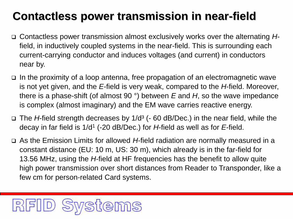
Contactless power transmission almost exclusively works over the alternating H-
field, in inductively coupled systems in the near-field. This is surrounding each
current-carrying conductor and induces voltages (and current) in conductors
near by.
In the proximity of a loop antenna, free propagation of an electromagnetic wave
is not yet given, and the E-field is very weak, compared to the H-field. Moreover,
there is a phase-shift (of almost 90 °) between E and H, so the wave impedance
is complex (almost imaginary) and the EM wave carries reactive energy.
The H-field strength decreases by 1/d³ (- 60 dB/Dec.) in the near field, while the
decay in far field is 1/d1 (-20 dB/Dec.) for H-field as well as for E-field.
As the Emission Limits for allowed H-field radiation are normally measured in a
constant distance (EU: 10 m, US: 30 m), which already is in the far-field for
13.56 MHz, using the H-field at HF frequencies has the benefit to allow quite
high power transmission over short distances from Reader to Transponder, like a
few cm for person-related Card systems.
Contactless power transmission in near-field
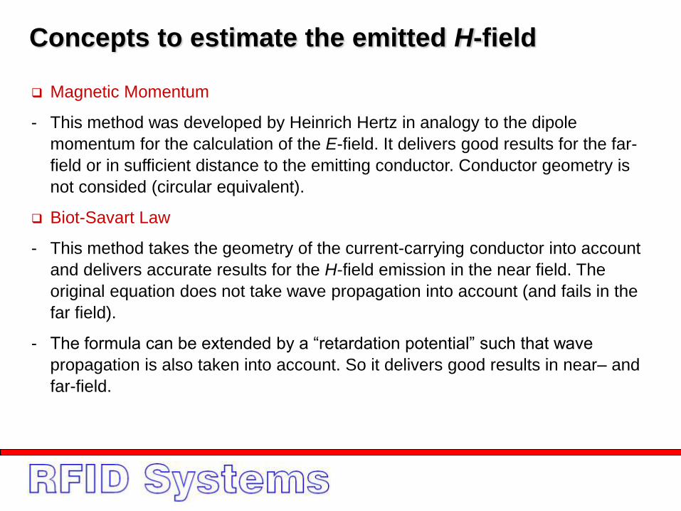
Concepts to estimate the emitted H-field
Magnetic Momentum
- This method was developed by Heinrich Hertz in analogy to the dipole
momentum for the calculation of the E-field. It delivers good results for the far-
field or in sufficient distance to the emitting conductor. Conductor geometry is
not consided (circular equivalent).
Biot-Savart Law
- This method takes the geometry of the current-carrying conductor into account
and delivers accurate results for the H-field emission in the near field. The
original equation does not take wave propagation into account (and fails in the
far field).
- The formula can be extended by a “retardation potential” such that wave
propagation is also taken into account. So it delivers good results in near– and
far-field.
page 6
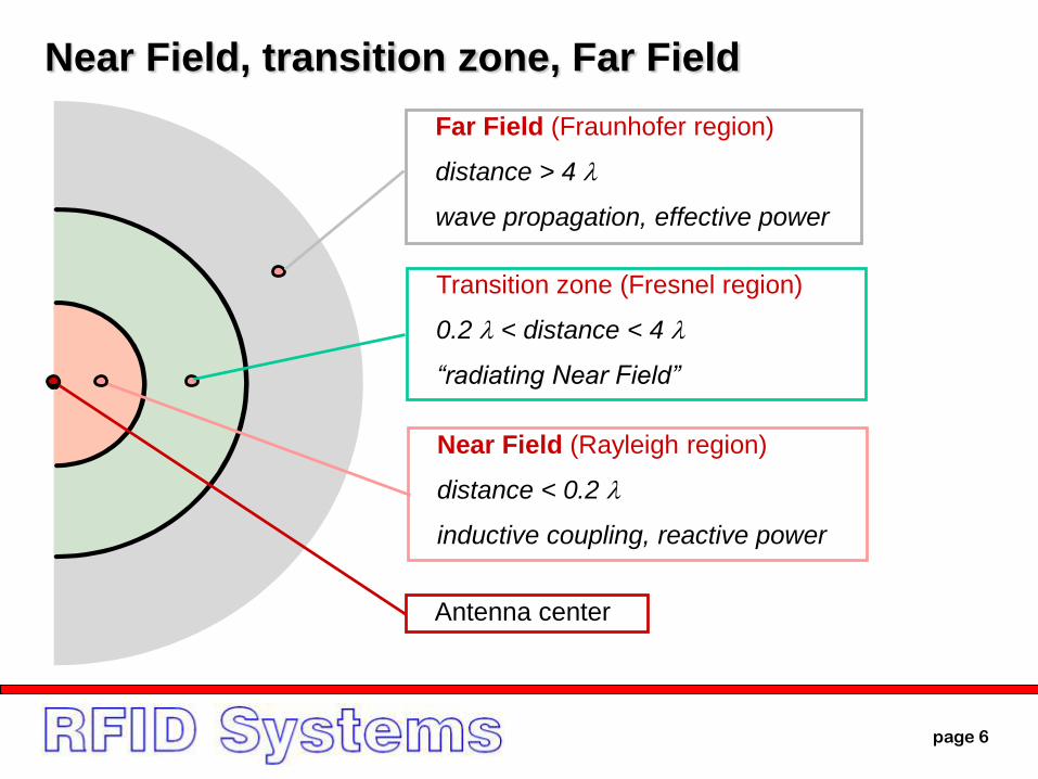
Near Field, transition zone, Far Field
Far Field (Fraunhofer region)
distance > 4 l
wave propagation, effective power
Transition zone (Fresnel region)
0.2 l < distance < 4 l
“radiating Near Field”
Near Field (Rayleigh region)
distance < 0.2 l
inductive coupling, reactive power
Antenna center
page 7
Estimating the emitted H-field independent of
antenna geometry (far field)
The Magnetic Momentum method
page 8
The magnetic momentum
Heinrich Hertz developed the method of the magnetic momentum to calculate
the H-field strength in space, in analog to the electric dipole momentum.
- It delivers good results in the far field of an antenna
- The magnetic momentum for a conductor loop of any shape is given by the
alternating current times the area inside the loop
AdImd
x
y
z
Loop-
antenna
Dipole-
antenna
- for a rectangular loop:- for a circular loop:
…current density times velocity
…direction from origin to space element
page 9
The magnetic momentum
Heinrich Hertz developed the method of the magnetic momentum to calculate
the H-field strength in space, in analog to the electric dipole momentum.
- It delivers good results in the far field of an antenna
- The magnetic momentum for a conductor loop of any shape is given by the
alternating current times the area inside the loop
AdImd
IrNAINmd 2
- In practice we find for the absolute of the momentum for a planar loop:
IblNAINmd
dVJrmd
2
1
- More general, for arbitrary current distribution in the space volume:
…space volume element dddrrdV sin2
r
vJ
…radian wavelength,
angular wavelength
page 10
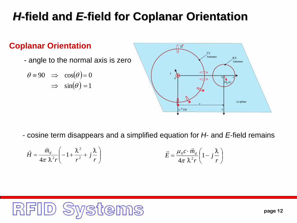
sin1cos2
4 2
2
2
2
2 rj
rrj
rr
mH d
sin1
4 2
0
rj
r
mcE d
H
EZ
l
2
- The H-field and the E-field (of a current-carrying conductor loop) in space can
be derived from the magnetic momentum for any point in space in spherical
coordinates by
z
x
y
H
E
r
I
Point in space
current-carrying
conductor loop
0
H-field expressed by the magnetic momentum
- The relation of E-field to H-field gives
the field impedance Z
page 11
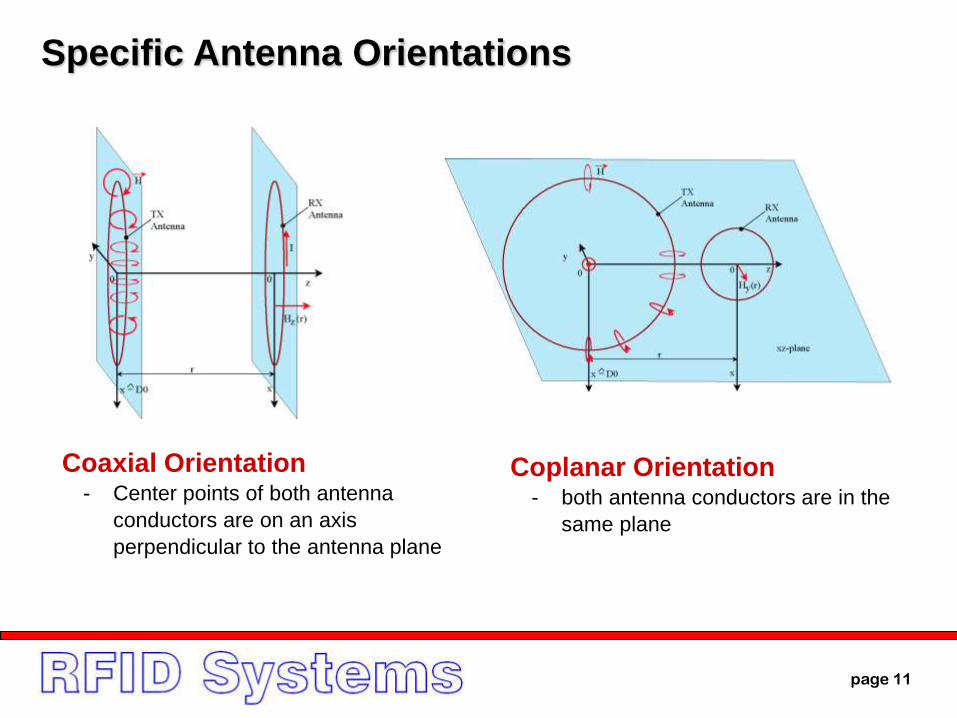
Specific Antenna Orientations
Coaxial Orientation- Center points of both antenna
conductors are on an axis
perpendicular to the antenna plane
Coplanar Orientation- both antenna conductors are in the
same plane
page 12
rj
rr
mH d
2
2
21
4
1sin
0cos90
rj
r
mcE d
1
4 2
0
H-field and E-field for Coplanar Orientation
Coplanar Orientation
- angle to the normal axis is zero
- cosine term disappears and a simplified equation for H- and E-field remains
page 13
4224
22
22
2
2
2
1
4
14
rrrr
m
rrr
mH
d
d
22
2
0
2
2
2
0
1
4
14
rrr
mc
rr
mcE
d
d
4224
34
0
2
20
2
2
2
2
0
1
1
14
14
rr
jrrZ
rj
r
rj
Z
rj
rr
m
rj
r
mc
H
EZ
d
d
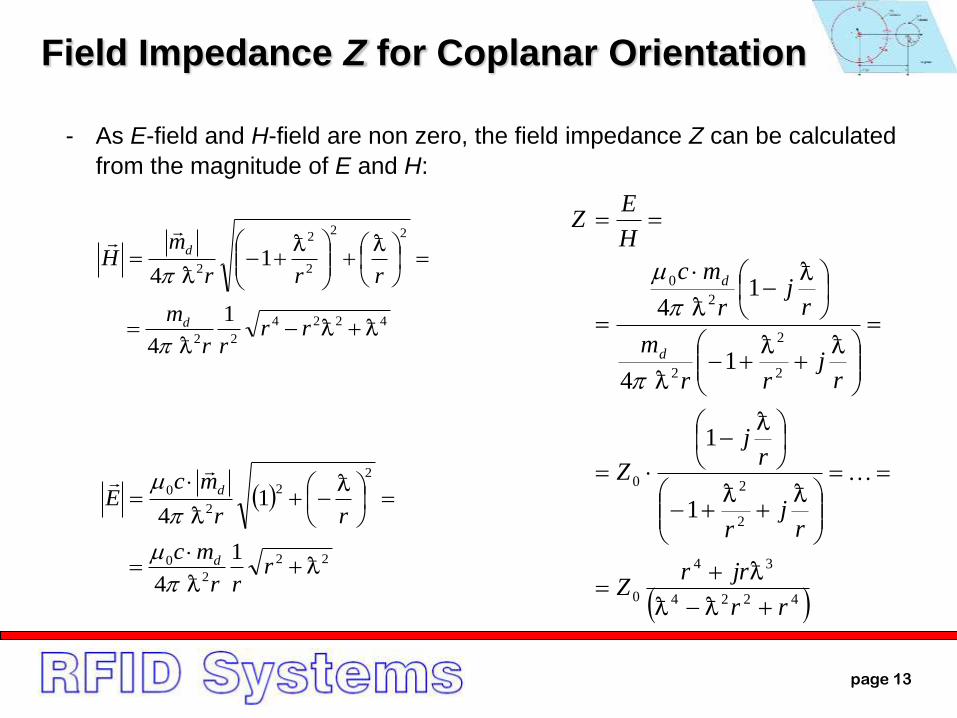
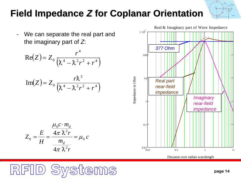
Field Impedance Z for Coplanar Orientation
- As E-field and H-field are non zero, the field impedance Z can be calculated
from the magnitude of E and H:
page 14
Field Impedance Z for Coplanar Orientation
- We can separate the real part and
the imaginary part of Z:
4224
4
0Rerr
rZZ
4224
3
0Imrr
rZZ
0.01 0.1 1 100.01
0.1
1
10
100
1 103
Real & Imaginary part of Wave Impedance
Distance over radian wavelength
Imped
ance
in O
hm
c
r
m
r
mc
H
EZ
d
d
0
2
2
0
0
4
4
377 Ohm
Imaginary
near-field
impedance
Real part
near-field
impedance

page 15
Field Impedance Z for Coplanar Orientation
4224
66
0
22 ImRe
rr
rrZ
H
EZZZ
- The magnitude of Z can be calculated
from real and imaginary part:
3771201
0
0
00
ccZ
- At the far field the field impedance Z
approximates the wave impedance Z0
0.01 0.1 1 1010
100
1 103
Magnitude of Field Impedance coplanar
Distance over radian wavelengthIm
ped
ance
in O
hm
377 Ohm
Magnitude
near-field
impedance
page 16
0sin
1cos0
rj
rr
mH d
2
2
24
20
00 E
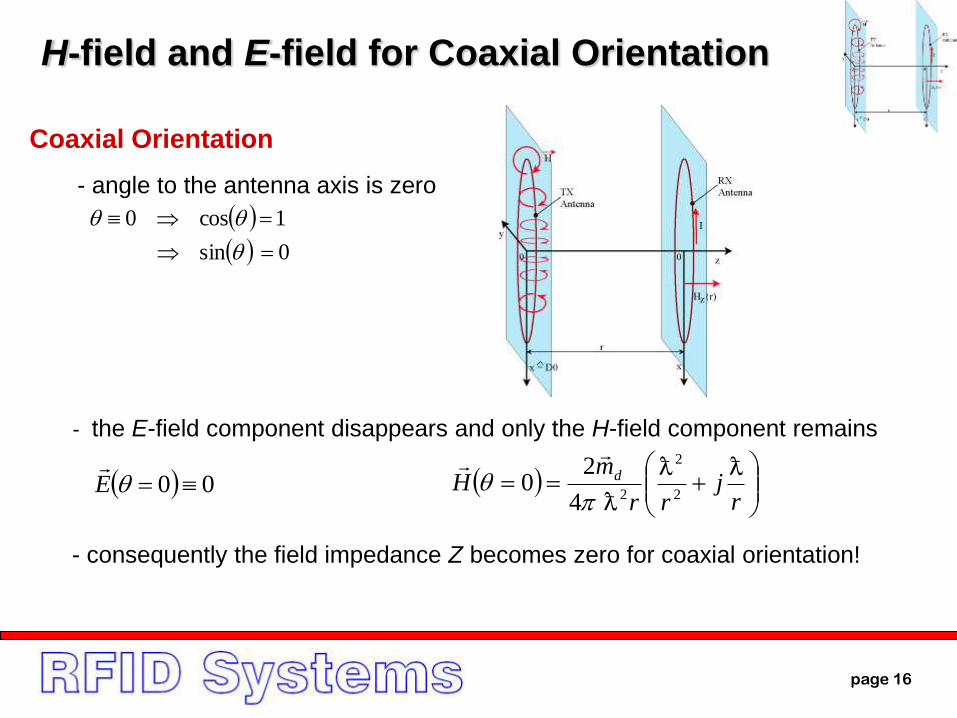
H-field and E-field for Coaxial Orientation
Coaxial Orientation
- angle to the antenna axis is zero
- the E-field component disappears and only the H-field component remains
- consequently the field impedance Z becomes zero for coaxial orientation!
page 17
rj
rr
mH d
2
2
24
20
224
32
22
2
2
2
22
1
2
4
2
ImRe
rr
m
rrr
m
H
d
d
rj
rr
mH d
2
2
21
490
4224
22
22
2
2
2
1
4
14
rrrr
m
rrr
mH
d
d
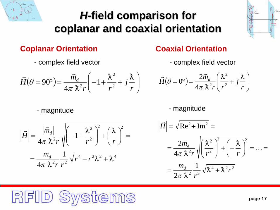
H-field comparison for
coplanar and coaxial orientation
- magnitude - magnitude
Coplanar Orientation
- complex field vector
Coaxial Orientation
- complex field vector
page 18
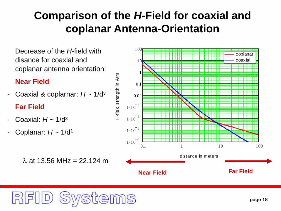
Comparison of the H-Field for coaxial and
coplanar Antenna-Orientation
Far FieldNear Field
Decrease of the H-field with
disance for coaxial and
coplanar antenna orientation:
Near Field
- Coaxial & coplarnar: H ~ 1/d³
Far Field
- Coaxial: H ~ 1/d³
- Coplanar: H ~ 1/d1
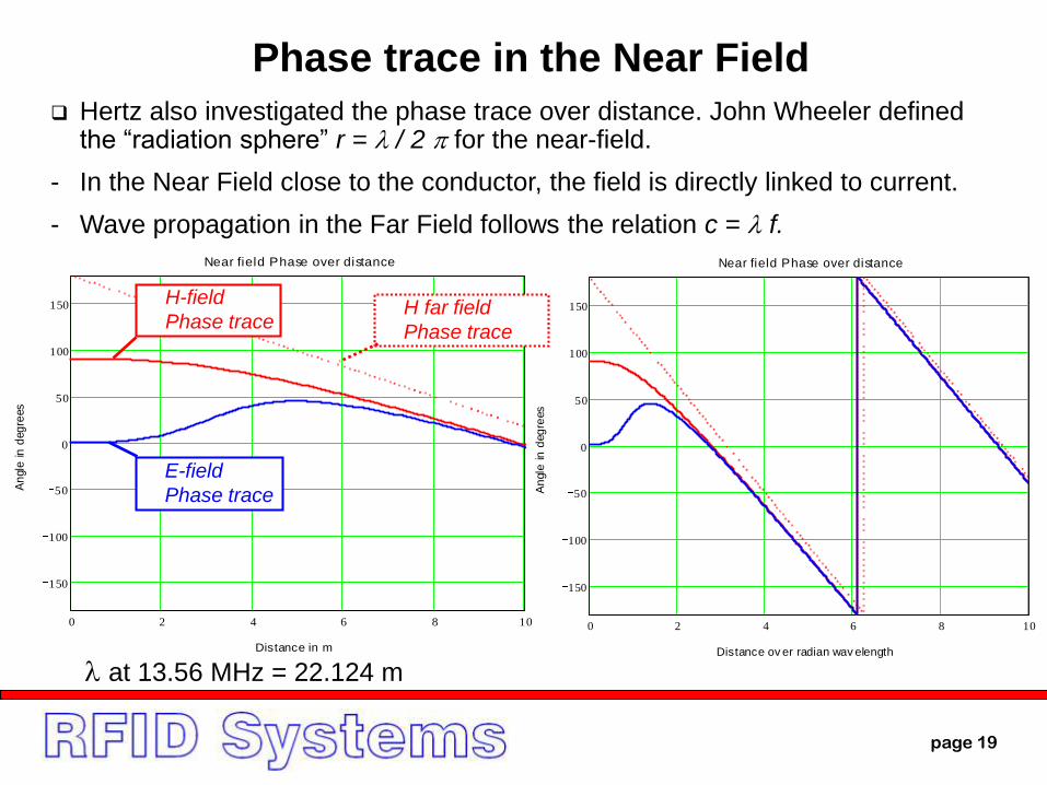
l at 13.56 MHz = 22.124 m
0.1 1 10 1001 10
6
1 105
1 104
1 103
0.01
0.1
1
10
100coplanar
coaxial
distance in meters
H-f
ield
str
en
gth
in
A/m
l at 13.56 MHz = 22.124 m
0 2 4 6 8 10
150
100
50
0
50
100
150
Near field Phase over distance
Distance in m
An
gle
in
deg
rees
page 19
E-field
Phase trace
H-field
Phase traceH far field
Phase trace
0 2 4 6 8 10
150
100
50
0
50
100
150
Near field Phase over distance
Distance ov er radian wav elength
An
gle
in
deg
rees
0 2 4 6 8 10
150
100
50
0
50
100
150
Near field Phase over distance
Distance in m
An
gle
in
deg
rees
Phase trace in the Near Field
Hertz also investigated the phase trace over distance. John Wheeler defined the “radiation sphere” r = l / 2 for the near-field.
- In the Near Field close to the conductor, the field is directly linked to current.
- Wave propagation in the Far Field follows the relation c = l f.
page 20
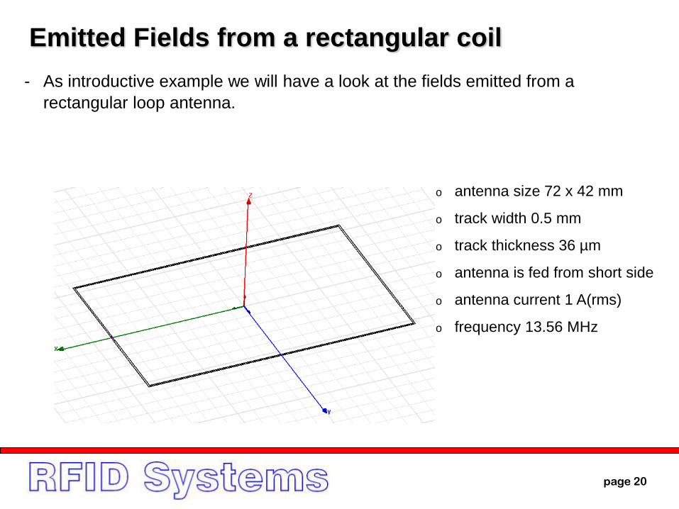
Emitted Fields from a rectangular coil
- As introductive example we will have a look at the fields emitted from a
rectangular loop antenna.
o antenna size 72 x 42 mm
o track width 0.5 mm
o track thickness 36 µm
o antenna is fed from short side
o antenna current 1 A(rms)
o frequency 13.56 MHz

page 21
H-field and E-field Magnitude

page 22
H-field and E-field Direction
electromagnetic wave in the far field
page 23
REF
ABSdB
H
HH log20 2010
dBH
REFABS HH
dBZ dB 5.51377log20,0
mVmAZHE LIMITLIMIT 377000377/10000
)/(5.111)(5.51)/(605.51,0 mVdBdBmAdBdBHZHE dBdBdBdB
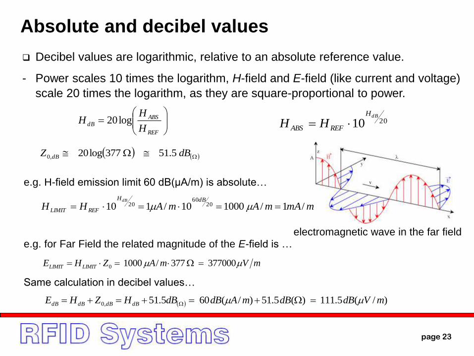
Absolute and decibel values
Decibel values are logarithmic, relative to an absolute reference value.
- Power scales 10 times the logarithm, H-field and E-field (like current and voltage)
scale 20 times the logarithm, as they are square-proportional to power.
e.g. H-field emission limit 60 dB(µA/m) is absolute…
mmAmAmAHHdBH
REFLIMIT
dB
/1/100010/110 2060
20
e.g. for Far Field the related magnitude of the E-field is …
Same calculation in decibel values…
x
y
z
Loop-
antenna
Dipole-
antenna
page 24
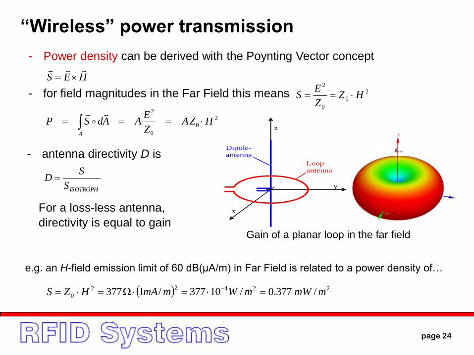
“Wireless” power transmission
2
0
0
2
HZZ
ES
22422
0 /377.0/10377/1377 mmWmWmmAHZS
HES
ISOTROPHS
SD
2
0
0
2
HZAZ
EAAdSP
A
- Power density can be derived with the Poynting Vector concept
- for field magnitudes in the Far Field this means
- antenna directivity D is
For a loss-less antenna,
directivity is equal to gainGain of a planar loop in the far field
e.g. an H-field emission limit of 60 dB(µA/m) in Far Field is related to a power density of…
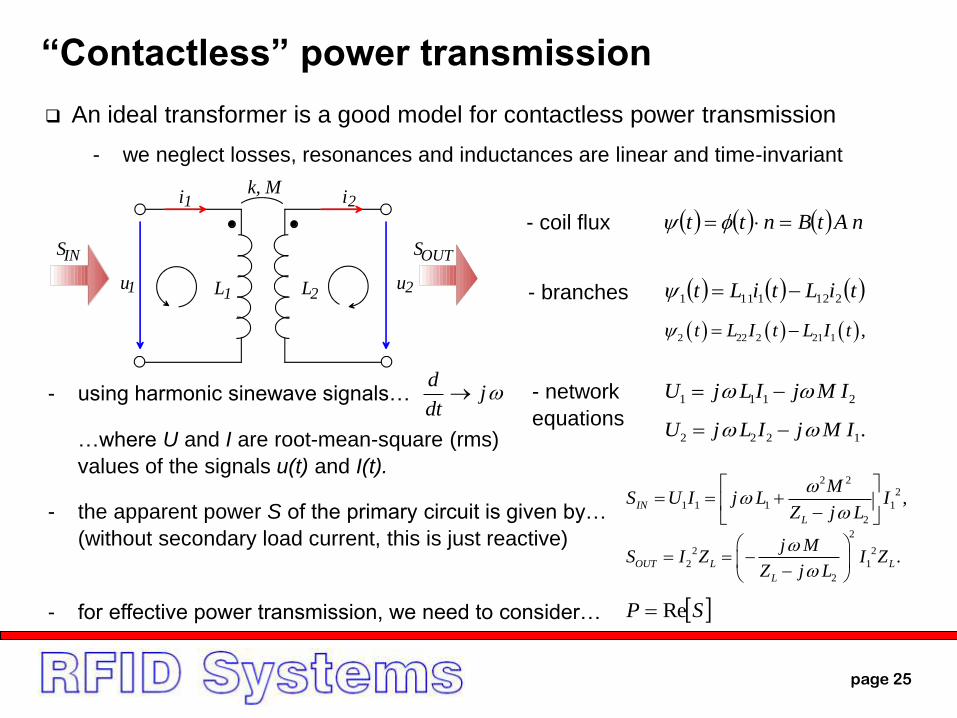
“Contactless” power transmission
An ideal transformer is a good model for contactless power transmission
- we neglect losses, resonances and inductances are linear and time-invariant
nAtBntt - coil flux
- branches
jdt
d- using harmonic sinewave signals… - network
equations…where U and I are root-mean-square (rms)
values of the signals u(t) and I(t).
- the apparent power S of the primary circuit is given by…
(without secondary load current, this is just reactive)
- for effective power transmission, we need to consider…
i1
L1u1
i2
L2u2
k, M
SIN SOUT
tiLtiLt 2121111
2111 IMjILjU
SP Re
2 22 2 21 1 ,t L I t L I t
2 2 2 1.U j L I j M I
2 22
1 1 1 1
2
,IN
L
MS U I j L I
Z j L
2
2 2
2 1
2
.OUT L L
L
j MS I Z I Z
Z j L
page 25

Summary Near Field, Far Field
distance32
ldistance3.0
2
l
l
2
02distanceD
l
2
02distanceD
Near Field Far Field
HE
0)(),( tHtE 0)(),( tHtE
Electromagnetic
Wave
Limit of field
region
Antenna
diameter D0
Phase-shift
in time
Spatial field
vectors
page 26
page 27
Calculating emitted alternating H-field close to the
conductor
Biot-Savart law
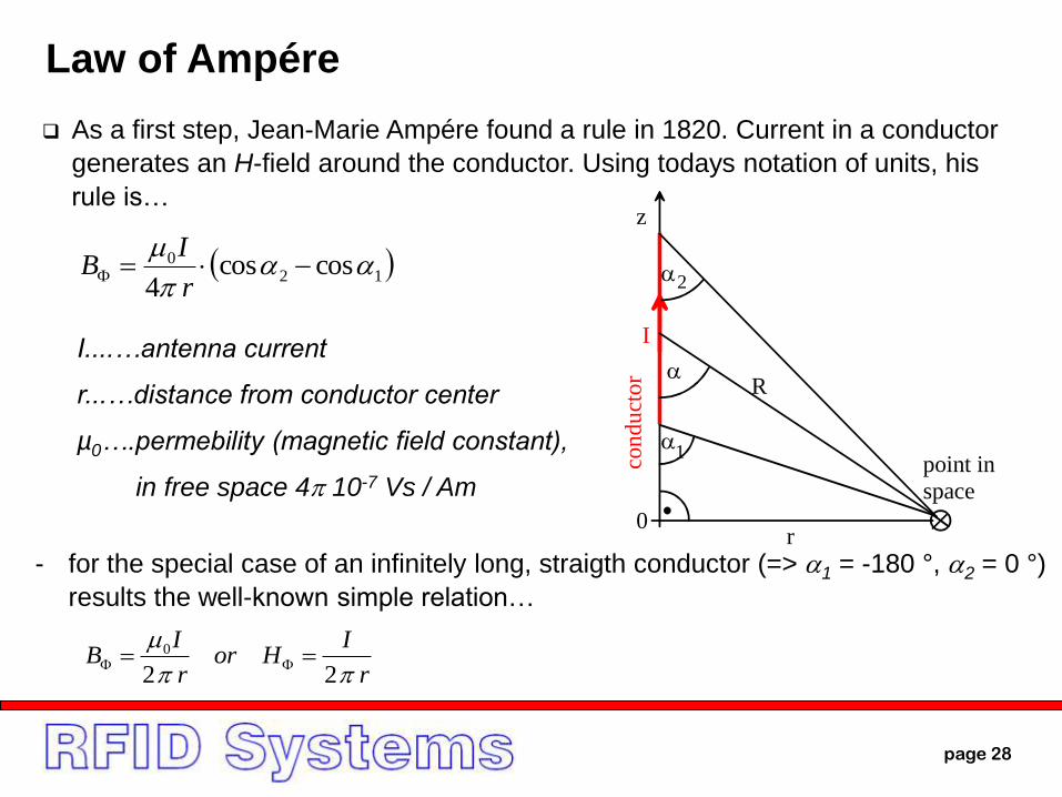
page 28
120 coscos
4
r
IB
I....…antenna current
r...…distance from conductor center
µ0….permebility (magnetic field constant),
in free space 4 10-7 Vs / Am
r
IHor
r
IB
22
0
Law of Ampére
As a first step, Jean-Marie Ampére found a rule in 1820. Current in a conductor
generates an H-field around the conductor. Using todays notation of units, his
rule is…
- for the special case of an infinitely long, straigth conductor (=> 1 = -180 °, 2 = 0 °)
results the well-known simple relation…
I
z
0
1
r
point in
space
R
2
con
du
cto
r
page 29
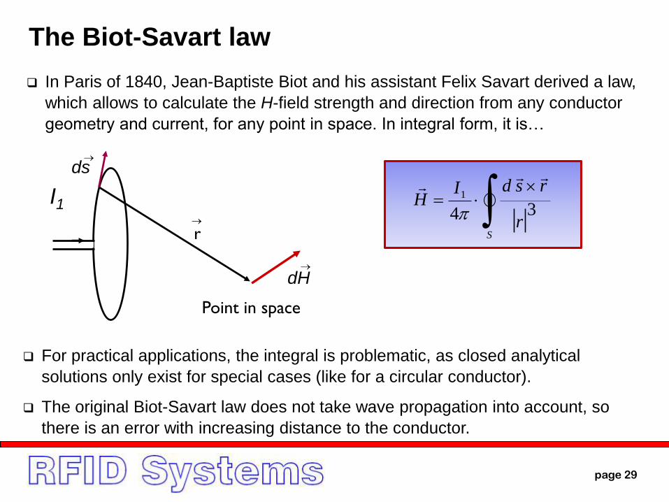
I1
r
ds
dH
Point in space
Sr
rsdIH
34
1
For practical applications, the integral is problematic, as closed analytical
solutions only exist for special cases (like for a circular conductor).
The original Biot-Savart law does not take wave propagation into account, so
there is an error with increasing distance to the conductor.
The Biot-Savart law
In Paris of 1840, Jean-Baptiste Biot and his assistant Felix Savart derived a law,
which allows to calculate the H-field strength and direction from any conductor
geometry and current, for any point in space. In integral form, it is…
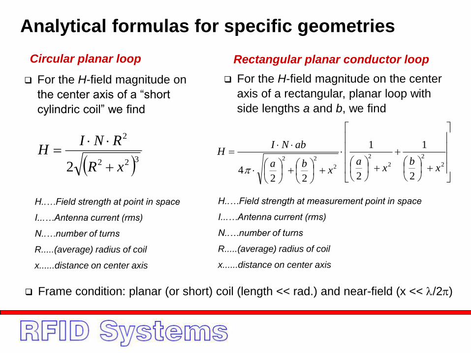
322
2
2 xR
RNIH
H..…Field strength at point in space
I...…Antenna current (rms)
N..…number of turns
R.....(average) radius of coil
x......distance on center axis
2
2
2
2
2
22
2
1
2
1
224 x
bx
ax
ba
abNIH
Analytical formulas for specific geometries
Circular planar loop Rectangular planar conductor loop
For the H-field magnitude on
the center axis of a “short
cylindric coil” we find
For the H-field magnitude on the center
axis of a rectangular, planar loop with
side lengths a and b, we find
H..…Field strength at measurement point in space
I...…Antenna current (rms)
N..…number of turns
R.....(average) radius of coil
x......distance on center axis
Frame condition: planar (or short) coil (length << rad.) and near-field (x << l/2)
page 31
dyyxxar
ir
eaIzyxH RSRS
SRSR
ri
ARRRz
SR
2
0
2)sin()cos(
1
4,,
dr
ir
ezzaIzyxH
SRSR
ri
RSARRRx
SR
2
0
2
1cos
4,,
dr
ir
ezzaIzyxH
SRSR
ri
RSARRRy
SR
2
0
2
1sin
4,,
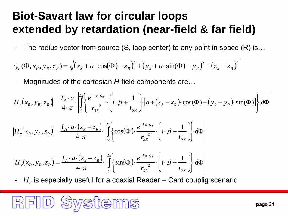
Biot-Savart law for circular loops
extended by retardation (near-field & far field)
- Magnitudes of the cartesian H-field components are…
- HZ is especially useful for a coaxial Reader – Card couplig scenario
222)sin(cos),,,( RSRSRSRRRSR zzyayxaxzyxr
- The radius vector from source (S, loop center) to any point in space (R) is…
page 32
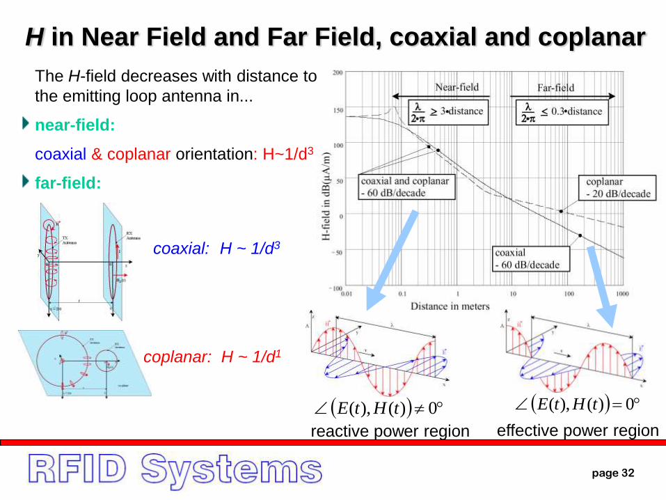
H in Near Field and Far Field, coaxial and coplanar
The H-field decreases with distance to
the emitting loop antenna in...
near-field:
coaxial & coplanar orientation: H~1/d3
far-field:
coaxial: H ~ 1/d3
coplanar: H ~ 1/d1
0)(),( tHtE 0)(),( tHtE
reactive power region effective power region
Two considerations using the Biot-Savart law
The Biot-Savart law gives accurate results for the Near Field and takes into
account the antenna geometry. So we will use it to make two considerations,
which are essential for size and shape of the loop antenna:
- Homogeneity of the emitted H-field
- Optimum (circular) antenna radius
The H-field can be described by a vector, which defines magnitude (strength)
and direction of the field, for any point in space. So in cartesian coordinates there
are 3 components, x, y, z. Of special interest is the case, where z is the loop
antenna axis, and x = y = 0.
Moreover, close to the conductor loop contributions of both conductors are in
opposite direction and same strength, so they cancel out. Considering HZ across
a plane over the loop antenna, one can find a H-field magnitude decrease over
the antenna center in short distance, and an increase in higher distance. In
between there is a specific distance to the antenna, where the H-field is equal
(homogenous). This distance is related to the antenna radius.
page 33
Optimum Loop Antenna radius
32222
3
322
32
xRxR
INR
xR
INRRH
dR
dRH
page 34
If we vary the loop antenna radius of the emitting antenna, for a fix distance to
the receive antenna in a coaxial antenna arrangement, we can find a maximum
of H-field. Of course, this maximum applies only for this fix distance.
So, there is an optimum loop antenna radius, related to the intended distance
regarding H-field emission. We can calculate the derivative of the equation for H-
field of circular antennas, to find this optimum radius:
Zeros of this function are at 2 x
So, the optimum radius regarding RF power requirements for H-field emission is
roughly 1.4 x the distance to the loop antenna center.
As a rule of thumb, the maximum distance should be roughly equal to the loop
antenna radius.
page 35
Network elements
Electrical Elements
page 36
sCZ
1
sLZ
Cj
CjZ
11
RZ
LjZ
RZ
jBGYjXRZ
R
jX
R
R
jX
jL
R
jX
-jC
U
I
U
I
U
I
00 cos tIti
00 cos tUtu
00 cos tIti
90cos 00 tUtu
00 cos tIti
90cos 00 tUtu
u(t)
i(t)t
t
t
u(t)
i(t)
i(t)
u(t)
Electrical Elements in overviewsymbol impedance phasor signal tracessignals
page 37
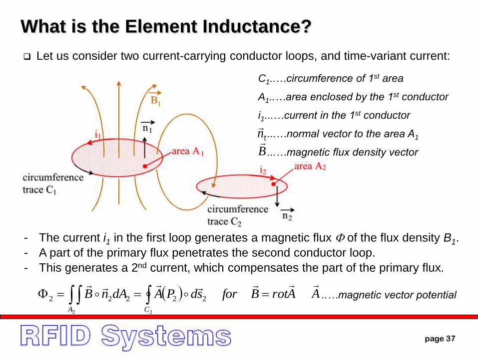
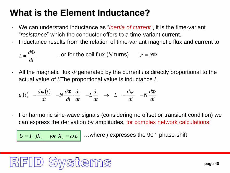
What is the Element Inductance?
Let us consider two current-carrying conductor loops, and time-variant current:
- The current i1 in the first loop generates a magnetic flux of the flux density B1.
- A part of the primary flux penetrates the second conductor loop.
- This generates a 2nd current, which compensates the part of the primary flux.
C1..…circumference of 1st area
A1..…area enclosed by the 1st conductor
i1...…current in the 1st conductor
....…normal vector to the area A1
...…magnetic flux density vector
ArotBforsdPAdAnBA C
2 2
22222
B1n
..…magnetic vector potentialA
page 38
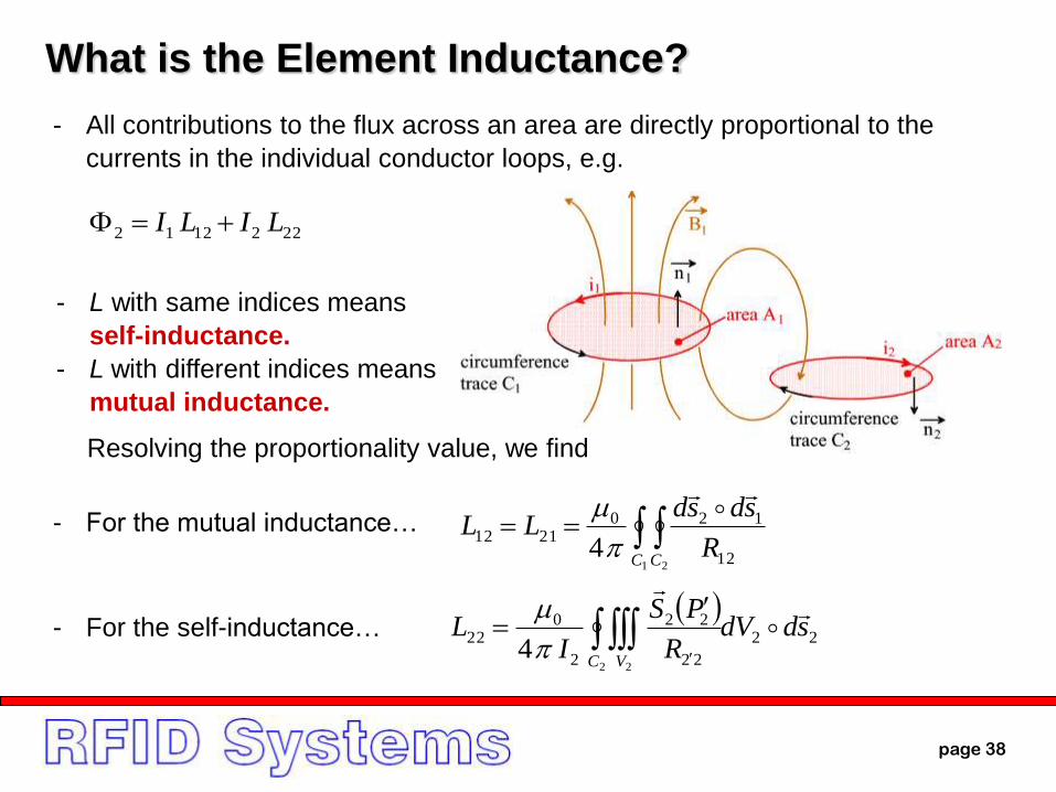
What is the Element Inductance?
- All contributions to the flux across an area are directly proportional to the
currents in the individual conductor loops, e.g.
2221212 LILI
1 212
1202112
4C C
R
sdsdLL
- L with same indices means
self-inductance.
- L with different indices means
mutual inductance.
Resolving the proportionality value, we find
- For the mutual inductance…
- For the self-inductance…
22
22
22
2
022
2 24
sddVR
PS
IL
C V
page 39
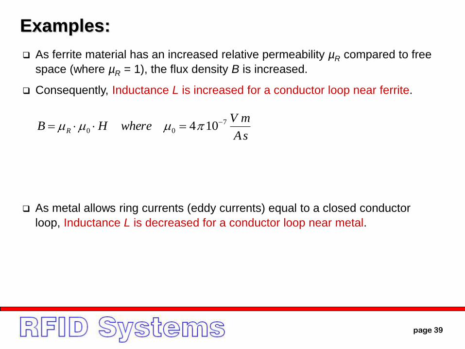
Examples:
As ferrite material has an increased relative permeability µR compared to free
space (where µR = 1), the flux density B is increased.
Consequently, Inductance L is increased for a conductor loop near ferrite.
sA
mVwhereHB R
7
00 104
As metal allows ring currents (eddy currents) equal to a closed conductor
loop, Inductance L is decreased for a conductor loop near metal.
…where j expresses the 90 ° phase-shift
page 40
What is the Element Inductance?
- We can understand inductance as “inertia of current”, it is the time-variant
“resistance” which the conductor offers to a time-variant current.
- Inductance results from the relation of time-variant magnetic flux and current to
dI
dL
- All the magnetic flux generated by the current i is directly proportional to the
actual value of i.The proportional value is inductance L
di
dN
di
dL
dt
diL
dt
di
di
dN
dt
tdtui
LXforjXIU LL
- For harmonic sine-wave signals (considering no offset or transient condition) we
can express the derivation by amplitudes, for complex network calculations:
N…or for the coil flux (N turns)
page 41
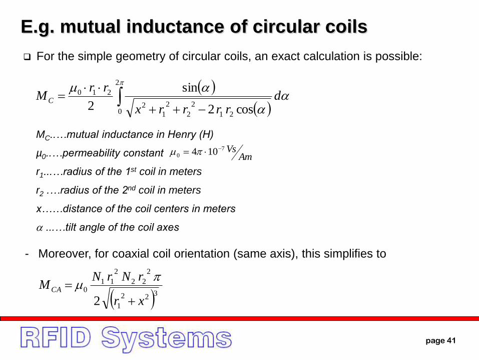
E.g. mutual inductance of circular coils
drrrrx
rrMC
2
0 21
2
2
2
1
2
210
cos2
sin
2
For the simple geometry of circular coils, an exact calculation is possible:
MC..…mutual inductance in Henry (H)
µ0..…permeability constant
r1...…radius of the 1st coil in meters
r2 .…radius of the 2nd coil in meters
x……distance of the coil centers in meters
...…tilt angle of the coil axes
322
1
2
22
2
110
2 xr
rNrNMCA
- Moreover, for coaxial coil orientation (same axis), this simplifies to
AmVs7
0 104
page 42
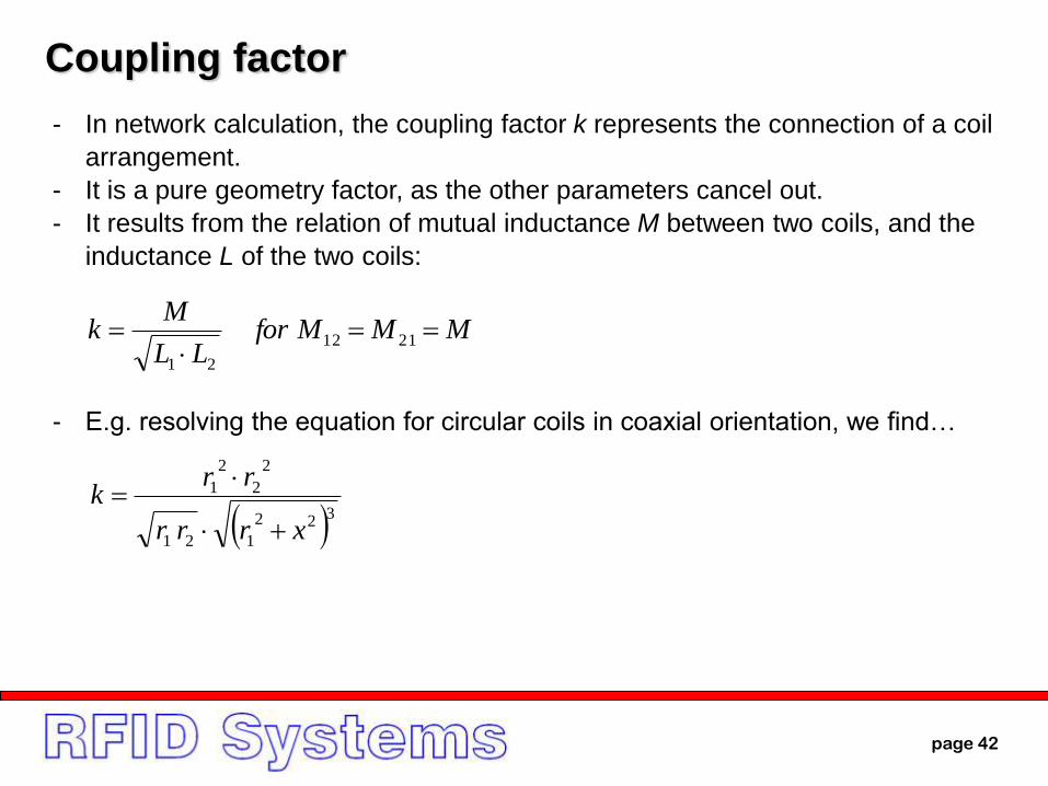
Coupling factor
- In network calculation, the coupling factor k represents the connection of a coil
arrangement.
- It is a pure geometry factor, as the other parameters cancel out.
- It results from the relation of mutual inductance M between two coils, and the
inductance L of the two coils:
MMMforLL
Mk
2112
21
- E.g. resolving the equation for circular coils in coaxial orientation, we find…
322
121
2
2
2
1
xrrr
rrk
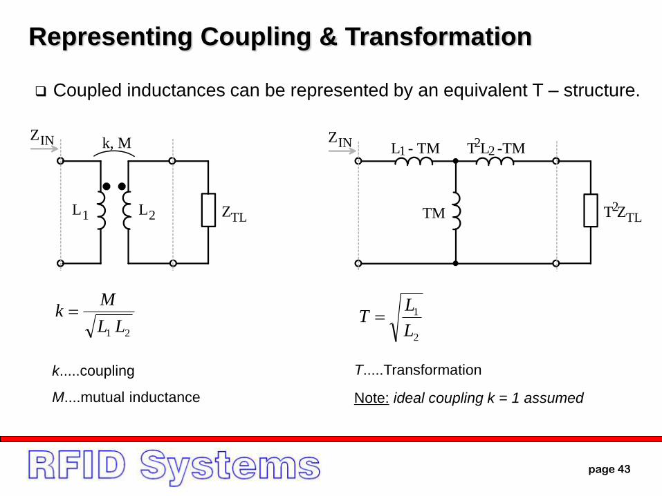
page 43
L1 L2 ZTL
ZIN k, M
Coupled inductances can be represented by an equivalent T – structure.
T ZTL
ZIN
TM
L - TM1 T L -TM22
2
21 LL
Mk
k.....coupling
M....mutual inductance
2
1
L
LT
T.....Transformation
Note: ideal coupling k = 1 assumed
Representing Coupling & Transformation
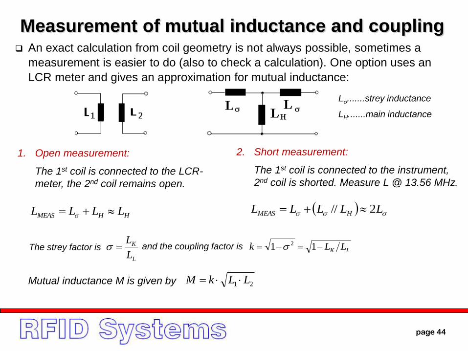
1. Open measurement:
The 1st coil is connected to the LCR-
meter, the 2nd coil remains open.
2. Short measurement:
The 1st coil is connected to the instrument,
2nd coil is shorted. Measure L @ 13.56 MHz.
HHMEAS LLLL LLLLL HMEAS 2//
The strey factor is
L
K
L
L and the coupling factor is
LK LLk 11 2
Mutual inductance M is given by 21 LLkM
L.......strey inductance
LH.......main inductance
An exact calculation from coil geometry is not always possible, sometimes a
measurement is easier to do (also to check a calculation). One option uses an
LCR meter and gives an approximation for mutual inductance:
Measurement of mutual inductance and coupling
page 44
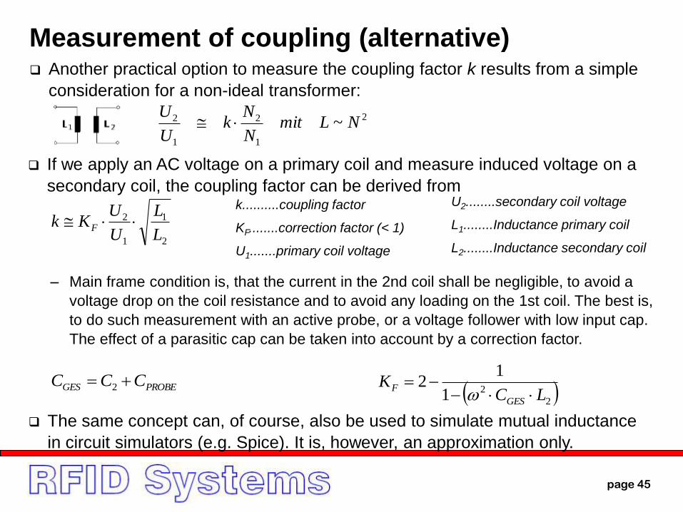
Measurement of coupling (alternative)
2
1
1
2
L
L
U
UKk F
k..........coupling factor
KF........correction factor (< 1)
U1.......primary coil voltage
U2........secondary coil voltage
L1........Inductance primary coil
L2........Inductance secondary coil
PROBEGES CCC 2 2
21
12
LCK
GES
F
2
1
2
1
2 ~ NLmitN
Nk
U
U
Another practical option to measure the coupling factor k results from a simple
consideration for a non-ideal transformer:
If we apply an AC voltage on a primary coil and measure induced voltage on a
secondary coil, the coupling factor can be derived from
The same concept can, of course, also be used to simulate mutual inductance
in circuit simulators (e.g. Spice). It is, however, an approximation only.
– Main frame condition is, that the current in the 2nd coil shall be negligible, to avoid a
voltage drop on the coil resistance and to avoid any loading on the 1st coil. The best is,
to do such measurement with an active probe, or a voltage follower with low input cap.
The effect of a parasitic cap can be taken into account by a correction factor.
page 45
page 46
What is the element Inductance?
Inductance (L) is a property of conductors and coils, relating
time-variant voltages to currents.
I
NL
8
0lL R…for the straight conductor…in Henry (H)
…where µ0 is the permeability constantAm
Vs7
0 104
Inductance also is an energy (W) storage and thus can be defined
22
2
ˆRMS
IM LI
iLW
Complex network calculation (without pre-charge)
sLIU
t
dttuL
ti1
dt
tdiLtu
sL
UI
)(ˆ: amplitudevaluepeakthemeansiNote
…for the long coill
ANL R 02
page 47
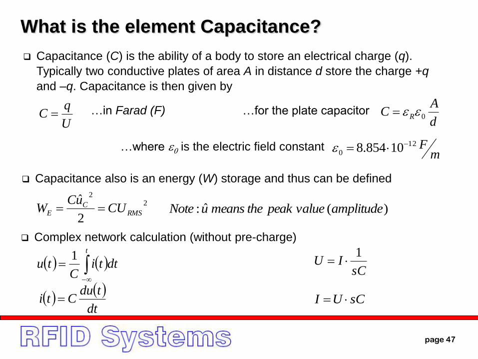
What is the element Capacitance?
Capacitance (C) is the ability of a body to store an electrical charge (q).
Typically two conductive plates of area A in distance d store the charge +q
and –q. Capacitance is then given by
U
qC
d
AC R 0…for the plate capacitor…in Farad (F)
…where 0 is the electric field constantm
F12
0 10854.8
Capacitance also is an energy (W) storage and thus can be defined
22
2
ˆRMS
CE CU
uCW
Complex network calculation (without pre-charge)
sCIU
1
t
dttiC
tu1
dt
tduCti sCUI
)(ˆ: amplitudevaluepeakthemeansuNote
page 48
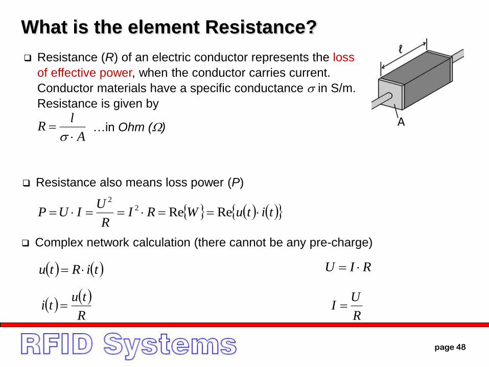
What is the element Resistance?
Resistance (R) of an electric conductor represents the loss
of effective power, when the conductor carries current.
Conductor materials have a specific conductance in S/m.
Resistance is given by
A
lR
…in Ohm ()
Complex network calculation (there cannot be any pre-charge)
tiRtu
R
tuti
RIU
R
UI
Resistance also means loss power (P)
tituWRIR
UIUP ReRe2
2
page 49
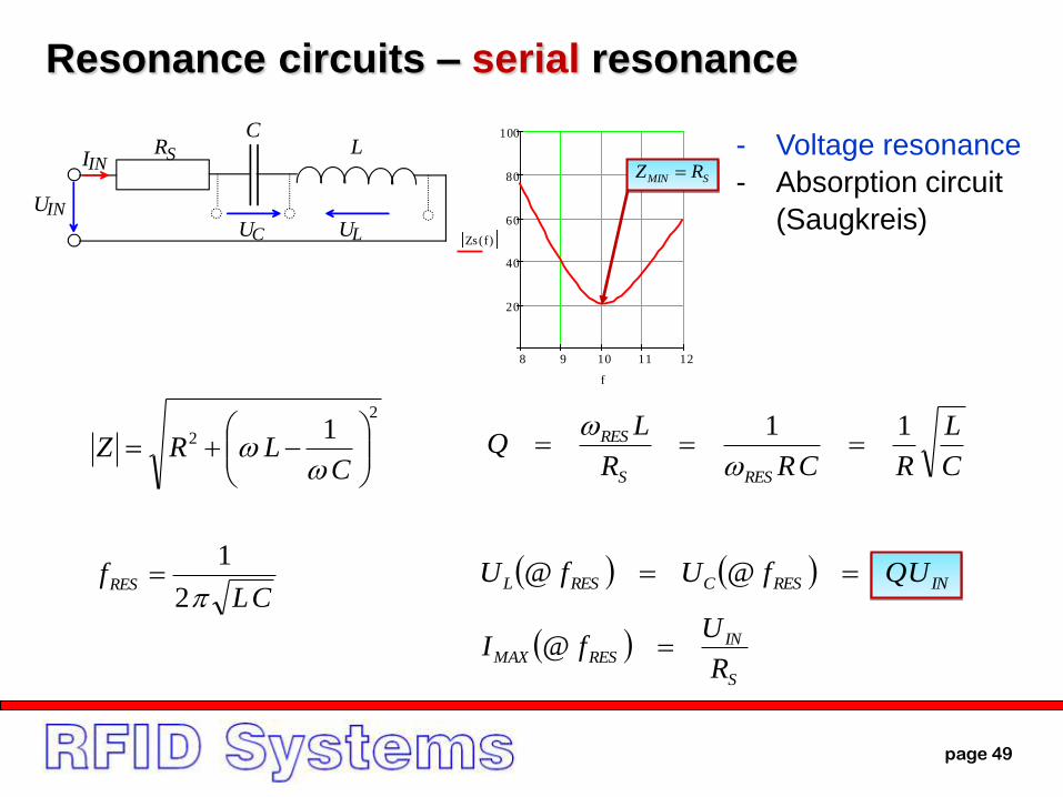
Resonance circuits – serial resonance
8 9 10 11 12
20
40
60
80
100
Zs f( )
f
2
2 1
CLRZ
C
L
RCRR
LQ
RESS
RES 11
CLfRES
2
1 INRESCRESL UQfUfU @@
S
INRESMAX
R
UfI @
UIN
RS
CL
IIN
UC UL
SMIN RZ
- Voltage resonance
- Absorption circuit
(Saugkreis)
page 50
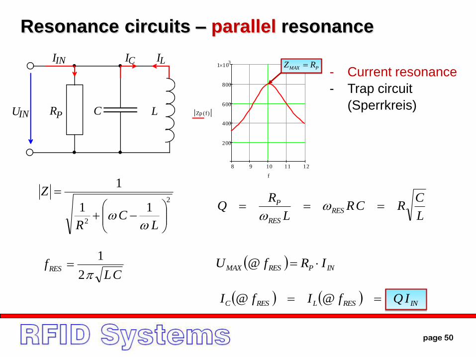
Resonance circuits – parallel resonance
8 9 10 11 12
200
400
600
800
1 103
Zp f( )
f
2
2
11
1
LC
R
Z
L
CRCR
L
RQ RES
RES
P
CLfRES
2
1 INPRESMAX IRfU @
INRESLRESC IQfIfI @@
LRPUIN C
IIN IC ILPMAX RZ
- Current resonance
- Trap circuit
(Sperrkreis)
page 5113th International Conference on Telecommunications (ConTEL), Graz, Austria
A AC
dAnDdt
ddAnJsdH
1
AC
dAnBdt
dsdE
2
03 A
dAnB
A V
dVdAnD
4
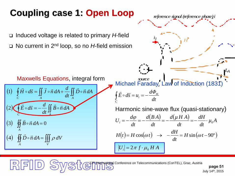
Maxwells Equations, integral form
Induced voltage is related to primary H-field
No current in 2nd loop, so no H-field emission
Michael Faraday, Law of Induction (1831)
dt
dΦusdE m
i
C
Aµ
dt
dH
dt
AHµd
dt
ABd
dt
dU i 0
Harmonic sine-wave flux (quasi-stationary)
90sincos tHdt
dHtHtH
AHfUi 02
LA
i1 H
i1
source
2nd coil
1st coil
reference signal (reference phase) i1
u2
u- 90 °
2
Coupling case 1: Open Loop
July 14th, 2015

page 5213th International Conference on Telecommunications (ConTEL), Graz, Austria
Rule of Lenz:
Current in 2nd loop generates H-field…
…that cancels out primary H-field (-180 °)
at the position of the 2nd coil
Dt
JHrot
1
Bt
Erot
2
03 Bdiv
Ddiv
4
Maxwells Equations, differential form
A closed loop of ideal conductor shorts induced voltage to zero.
This current in the 2nd loop is shifted by – 90 ° to an induced
voltage (which is – 90 ° shifted to primary current), so in total the
2nd current is – 180 ° shifted versus the primary current.
A resistance in series to the inductance allows some (induced)
voltage drop – the remaining voltage is shorted and
compensates partly the primary H-field at the second position.
LA RA
i 2
i2
i1 H- 180 °
i2
i1
source
2nd coil
1st coil
reference signal (reference phase) i 1Coupling case 2: Closed Loop
July 14th, 2015
12th International Conference on Telecommunications (ConTEL), Graz, Austria
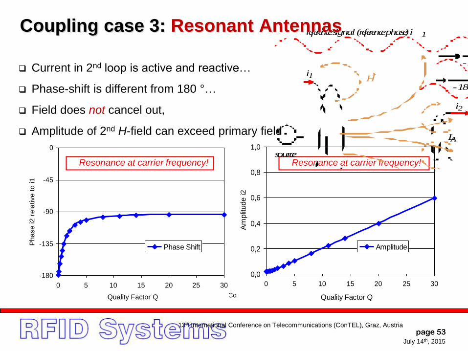
Current in 2nd loop is active and reactive…
Phase-shift is different from 180 °…
Field does not cancel out,
Amplitude of 2nd H-field can exceed primary field
-180
-135
-90
-45
0
0 5 10 15 20 25 30
Quality Factor Q
Ph
ase
i2
re
lative
to
i1
Phase Shift
0,0
0,2
0,4
0,6
0,8
1,0
0 5 10 15 20 25 30
Quality Factor Q
Am
plit
ude i2
Amplitude
Resonance at carrier frequency! Resonance at carrier frequency!
LA RC AA
i2
i2C i2R
i1 H
- 90 °
- 180 °i2R
i2C
i1
source
2nd coil
1st coil
reference signal (reference phase) i 1Coupling case 3: Resonant Antennas
page 53July 14th, 2015
13th International Conference on Telecommunications (ConTEL), Graz, Austria
page 54
Practical realization, how to measure the main
property, and some dependencies
Electrical Components
page 55
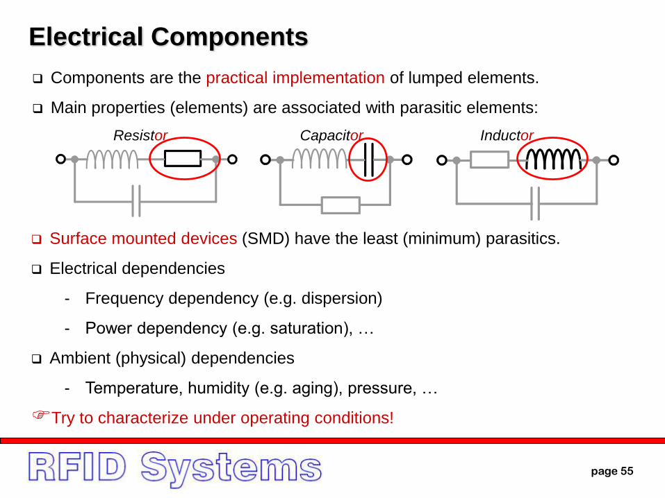
Electrical Components
Components are the practical implementation of lumped elements.
Main properties (elements) are associated with parasitic elements:
Surface mounted devices (SMD) have the least (minimum) parasitics.
Electrical dependencies
- Frequency dependency (e.g. dispersion)
- Power dependency (e.g. saturation), …
Ambient (physical) dependencies
- Temperature, humidity (e.g. aging), pressure, …
Try to characterize under operating conditions!
Resistor Capacitor Inductor
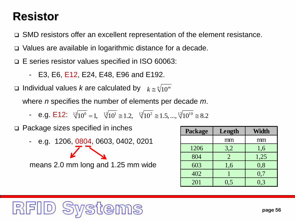
page 56
Resistor
SMD resistors offer an excellent representation of the element resistance.
Values are available in logarithmic distance for a decade.
E series resistor values specified in ISO 60063:
- E3, E6, E12, E24, E48, E96 and E192.
Individual values k are calculated by
where n specifies the number of elements per decade m.
- e.g. E12:
Package sizes specified in inches
- e.g. 1206, 0804, 0603, 0402, 0201
n mk 10
2.810...,,5.110,2.110,110 12 1012 212 112 0
means 2.0 mm long and 1.25 mm wide
Package Length Width
mm mm
1206 3,2 1,6
804 2 1,25
603 1,6 0,8
402 1 0,7
201 0,5 0,3
page 57
Capacitor
Capacitors can be a similar good representation of the element capacitance, if
the dielectric material is choosen right. COG or NP0 for SMD are good HF Caps.
The Electonics Industries Alliance (EIA) standardised 3 capacitor classes:
- Class 1: HF capacitors (typically ceramic) with high parameter stability
- Class 2: High volume efficiency capacitors (for buffers,…)
- Class 3: Volume efficiency ceramic caps (typ. – 22…+ 56 % cap over 10...55 °C)
- Class 4: Semiconductor caps
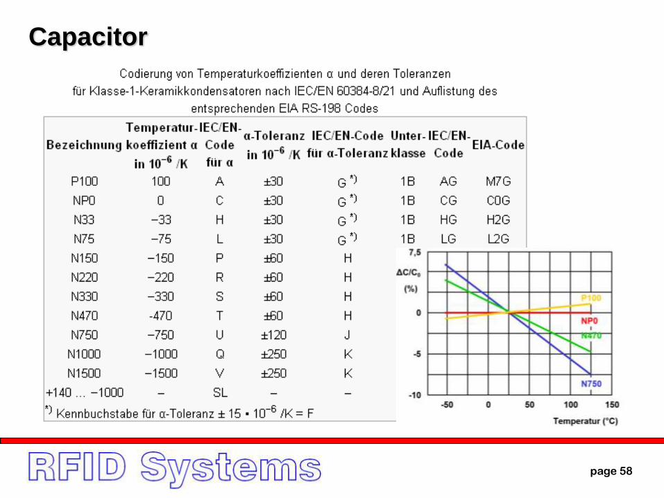
Class 1 ceramic capacitors are classified for temperature dependency in a
frequency range
- IEC/EN 60384-8/24 means 2-digit code, EIA RS-198 means 3 digit code
- NPO means zero gradient and +/-15 x 106 / K tolerance. EIA code is C0G,
IEC/EN code is C0
The EIA ceased operations in 2011, the Electronic Components Industry
Association (ECIA) will continue EIA standards maintenance.
page 58
Capacitor
page 59
Inductor
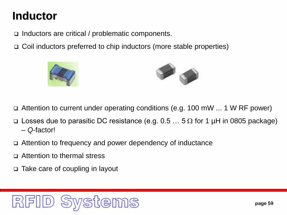
Inductors are critical / problematic components.
Coil inductors preferred to chip inductors (more stable properties)
Attention to current under operating conditions (e.g. 100 mW ... 1 W RF power)
Losses due to parasitic DC resistance (e.g. 0.5 … 5 for 1 µH in 0805 package)
– Q-factor!
Attention to frequency and power dependency of inductance
Attention to thermal stress
Take care of coupling in layout
page 60
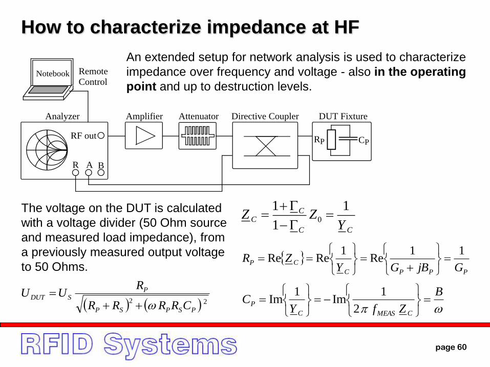
How to characterize impedance at HF
RF out
R A B
Analyzer Amplifier Directive Coupler DUT FixtureAttenuator
Notebook Remote
Control
CPRP
CC
CC
YZZ
1
1
10
PPPC
CPGjBGY
ZR11
Re1
ReRe
B
ZfYC
CMEASC
P
2
1Im
1Im 22
PSPSP
PSDUT
CRRRR
RUU
The voltage on the DUT is calculated
with a voltage divider (50 Ohm source
and measured load impedance), from
a previously measured output voltage
to 50 Ohms.
An extended setup for network analysis is used to characterize
impedance over frequency and voltage - also in the operating
point and up to destruction levels.
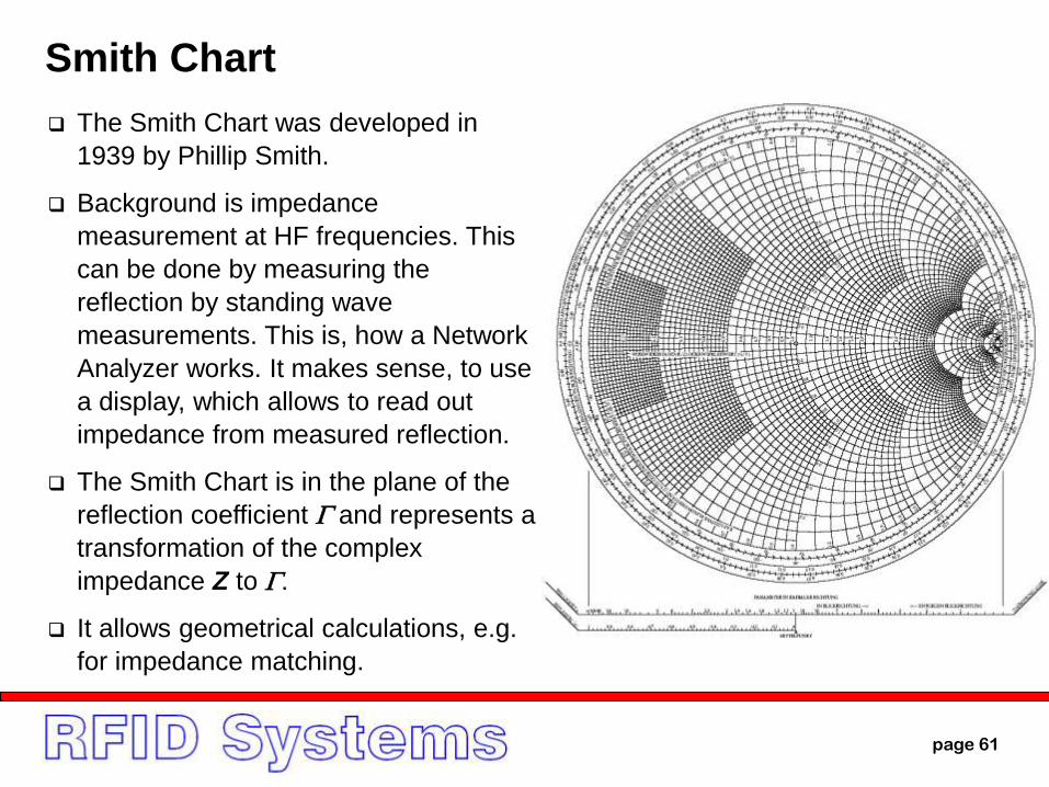
Smith Chart
page 61
The Smith Chart was developed in
1939 by Phillip Smith.
Background is impedance
measurement at HF frequencies. This
can be done by measuring the
reflection by standing wave
measurements. This is, how a Network
Analyzer works. It makes sense, to use
a display, which allows to read out
impedance from measured reflection.
The Smith Chart is in the plane of the
reflection coefficient and represents a
transformation of the complex
impedance Z to .
It allows geometrical calculations, e.g.
for impedance matching.
page 62
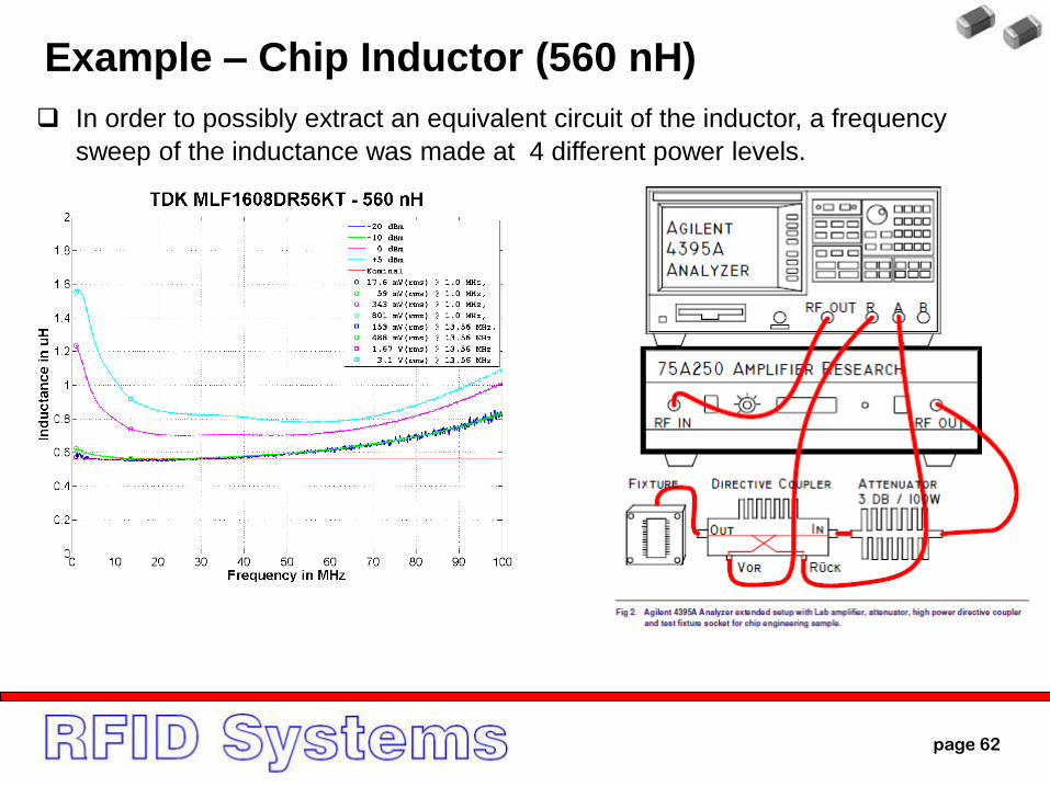
Example – Chip Inductor (560 nH)
In order to possibly extract an equivalent circuit of the inductor, a frequency
sweep of the inductance was made at 4 different power levels.
page 63
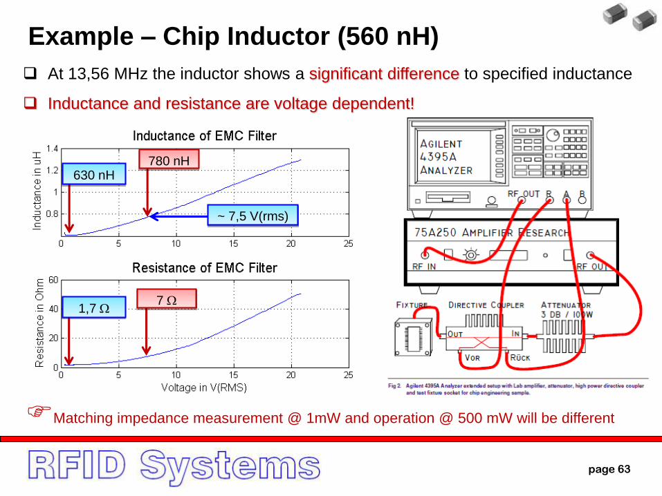
At 13,56 MHz the inductor shows a significant difference to specified inductance
Inductance and resistance are voltage dependent!
Matching impedance measurement @ 1mW and operation @ 500 mW will be different
630 nH
1,7
780 nH
7
~ 7,5 V(rms)
Example – Chip Inductor (560 nH)
page 64
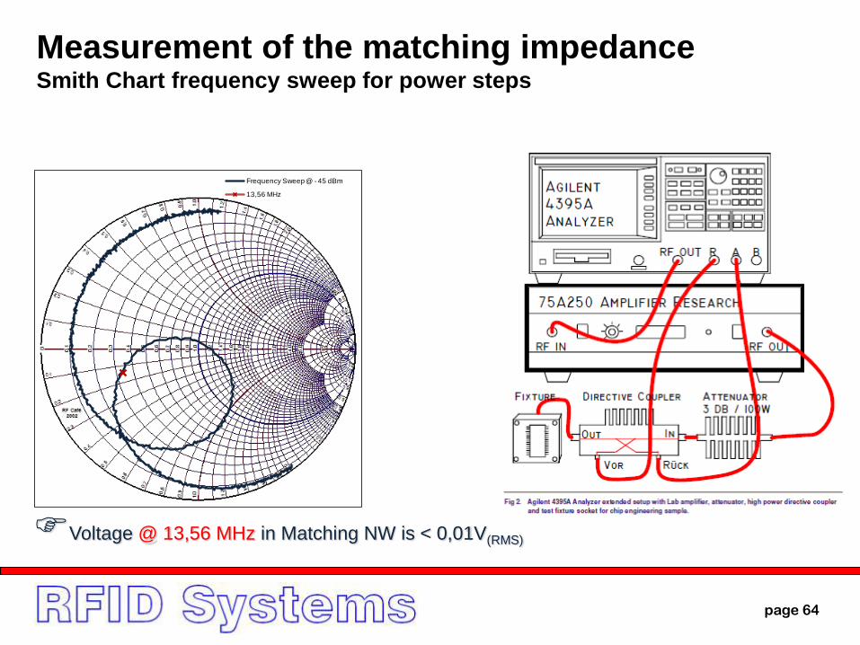
Measurement of the matching impedance Smith Chart frequency sweep for power steps
Voltage @ 13,56 MHz in Matching NW is < 0,01V(RMS)
Frequency Sweep @ - 45 dBm
13,56 MHz
page 65
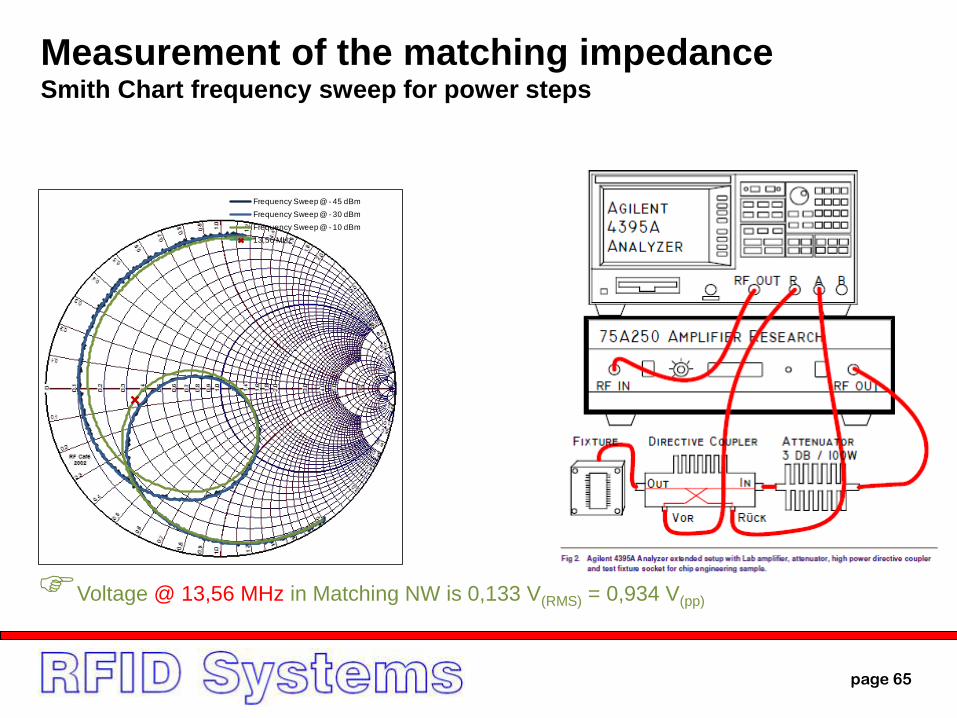
Measurement of the matching impedance Smith Chart frequency sweep for power steps
Voltage @ 13,56 MHz in Matching NW is 0,133 V(RMS) = 0,934 V(pp)
Frequency Sweep @ - 45 dBm
Frequency Sweep @ - 30 dBm
Frequency Sweep @ - 10 dBm
13,56 MHz
page 66
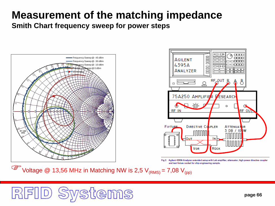
Measurement of the matching impedance Smith Chart frequency sweep for power steps
Frequency Sweep @ - 45 dBm
Frequency Sweep @ - 30 dBm
Frequency Sweep @ - 10 dBm
Frequency Sweep @ 0 dBm
13,56 MHz
Voltage @ 13,56 MHz in Matching NW is 2,5 V(RMS) = 7,08 V(pp)
page 67
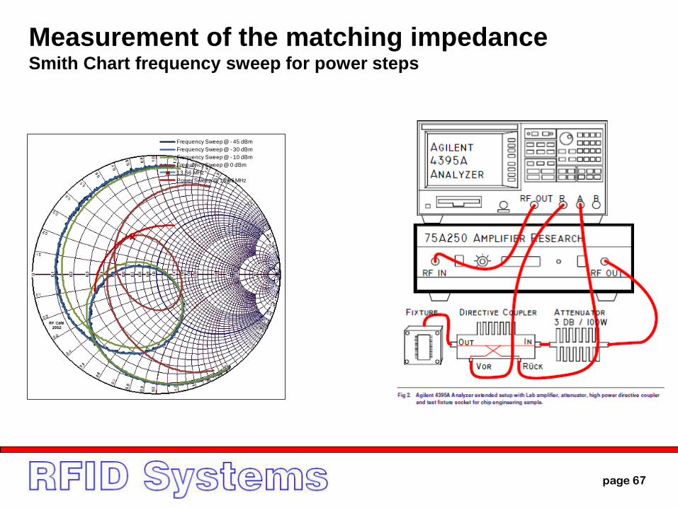
Measurement of the matching impedance Smith Chart frequency sweep for power steps
Frequency Sweep @ - 45 dBm
Frequency Sweep @ - 30 dBm
Frequency Sweep @ - 10 dBm
Frequency Sweep @ 0 dBm
13,56 MHz
Power Sweep @ 13,56 MHz
page 68
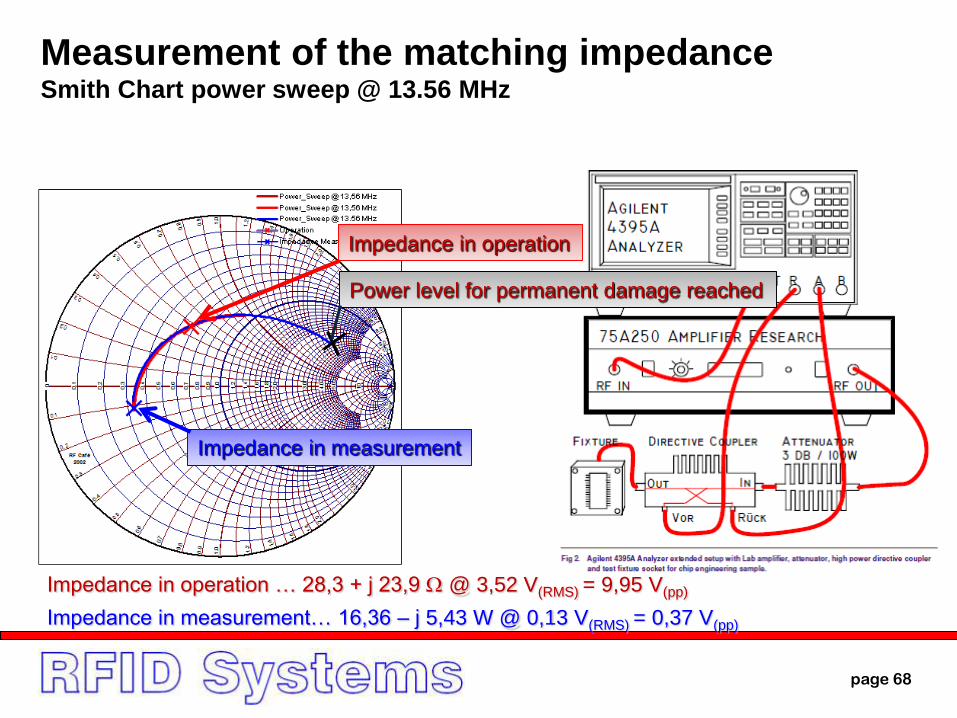
Measurement of the matching impedance Smith Chart power sweep @ 13.56 MHz
Impedance in operation
Impedance in measurement
Impedance in operation … 28,3 + j 23,9 @ 3,52 V(RMS) = 9,95 V(pp)
Impedance in measurement… 16,36 – j 5,43 W @ 0,13 V(RMS) = 0,37 V(pp)
Power level for permanent damage reached
page 69
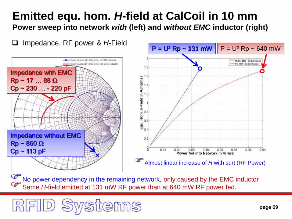
Emitted equ. hom. H-field at CalCoil in 10 mmPower sweep into network with (left) and without EMC inductor (right)
No power dependency in the remaining network, only caused by the EMC inductor
Same H-field emitted at 131 mW RF power than at 640 mW RF power fed.
Impedance with EMC
Rp ~ 17 … 88
Cp ~ 230 … - 220 pF
Impedance without EMC
Rp ~ 860
Cp ~ 113 pF
Almost linear increase of H with sqrt (RF Power)
P = U² Rp ~ 640 mWP = U² Rp ~ 131 mW Impedance, RF power & H-Field
page 70
Thank you for your
Audience!
Please feel free to ask questions...
page 71
References
Electromagnetic fields and waves, P. Lorrain, D. P. Carson, F. Lorrain, F. H.
Freeman & Co, New York, ISBN 0-716-71823-5
Strahlen, Wellen, Felder, N. Leitgeb, ISBN 3-13-750601-8
D. H. Werner, “An exact integration procedure for Vector Potentials of thin
circular loop antennas”, IEEE Transactions on Antennas and Propagation, Vol.
44, No 2, Feb. 1999
A. Oppenheim, R. W. Schäfer, J. R. Buck, Discrete-Time Signal Processing, 2nd
ed., Prentice Hall, ISBN-10: 8131704920, 1999
F. E. Terman, “Network Theory, Filters and Equalizers”, Proceedings of the I. R.
E., pp. 164-175, April 1943
J. Clerk Maxwell, “A Treatise on Electricity and Magnetism, 3rd ed., Vol. 2,
Oxford: Claendon, 1892
D. E. Scott, An Introduction to Circuit Analysis, McGraw-Hill International Edition,
ISBN 0-07-056127-3, 1987