05 algorithms for centrality indices

8/3/2019 05 Algorithms for Centrality Indices

http://slidepdf.com/reader/full/05-algorithms-for-centrality-indices 1/21

4 Algorithms for Centrality Indices

Riko Jacob,∗ Dirk Kosch¨ utzki, Katharina Anna Lehmann, Leon Peeters,∗

and Dagmar Tenfelde-Podehl

The usefulness of centrality indices stands or falls with the ability to computethem quickly. This is a problem at the heart of computer science, and muchresearch is devoted to the design and analysis of efficient algorithms. For example,

shortest-path computations are well understood, and these insights are easilyapplicable to all distance based centrality measures. This chapter is concernedwith algorithms that efficiently compute the centrality indices of the previouschapters.

Most of the distance based centralities can be computed by directly evaluat-ing their definition. Usually, this naıve approach is reasonably efficient once allshortest path distances are known. For example, the closeness centrality requiresto sum over all distances from a certain vertex to all other vertices. Given a ma-trix containing all distances, this corresponds to summing the entries of one rowor column. Computing all closeness values thus traverses the matrix once com-pletely, taking n2 steps. Computing the distance matrix using the fastest knownalgorithms will take between n2 and n3 steps, depending on the algorithm, andon the possibility to exploit the special structure of the network. Thus, comput-ing the closeness centrality for all vertices can be done efficiently in polynomialtime. Nevertheless, for large networks this can lead to significant computationtimes, in which case a specialized algorithm can be the crucial ingredient for an-alyzing the network at hand. However, even a specialized exact algorithm mightstill be too time consuming for really large networks, such as the Web graph. So,for such huge networks it is reasonable to approximate the outcome with veryfast, preferably linear time, algorithms.

Another important aspect of real life networks is that they frequently changeover time. The most prominent example of this behavior is the Web graph.Rather than recomputing all centrality values from scratch after some changes,we prefer to somehow reuse the previous computations. Such dynamic algorithmsare not only valuable in a changing environment. They can also increase per-formance for vitality based centrality indices, where the definition requires torepeatedly remove an element from the network. For example, dynamic all-pairsshortest paths algorithms can be used in this setting.

This chapter not only lists the known results, but also provides the ideasthat make such algorithms work. To that end, Section 4.1 recapitulates somebasic shortest paths algorithms, to provide the background for the more special-

∗ Lead authors

U. Brandes and T. Erlebach (Eds.): Network Analysis, LNCS 3418, pp. 62–82, 2005.c Springer-Verlag Berlin Heidelberg 2005



4 Algorithms for Centrality Indices 63

ized centrality algorithms presented in Section 4.2. Next, Section 4.3 describesfast approximation algorithms for closeness centrality as well as for web central-ities. Finally, algorithms for dynamically changing networks are considered inSection 4.4.

4.1 Basic Algorithms

Several good text books on basic graph algorithms are available, such as Ahuja,Magnanti, and Orlin [6], and Cormen, Leiserson, Rivest, and Stein [133]. Thissection recapitulates some basic and important algorithmic ideas, to provide abasis for the specific centrality algorithms in Section 4.2. Further, we brieflyreview the running times of some of the algorithms to indicate how computa-

tionally expensive different centrality measures are, especially for large networks.

4.1.1 Shortest Paths

The computation of the shortest-path distances between one specific vertex,called the source, and all other vertices is a classical algorithmic problem, knownas the Single Source Shortest Path (SSSP) problem.

Dijkstra [146] provided the first polynomial-time algorithm for the SSSPfor graphs with non-negative edge weights. The algorithm maintains a set of

shortest-path labels d(s, v) denoting the length of the shortest path found so-farbetween s and v. These labels are initialized to infinity, since no shortest pathsare known when the algorithm starts. The algorithm further maintains a list P of permanently labeled vertices, and a list T of temporarily labeled vertices. Fora vertex v ∈ P , the label d(s, v) equals the shortest-path distance between s andv, whereas for vertices v ∈ T the labels d(s, v) are upper bounds (or estimates)on the shortest-path distances.

The algorithm starts by marking the source vertex s as permanent and in-serting it into P , scanning all its neighbors N (s), and setting the labels for the

neighbors v ∈ N (s) to the edge lengths: d(s, v) = ω(s, v). Next, the algorithmrepeatedly removes a non-permanent vertex v with minimum label d(s, v) fromT , marks v as permanent, and scans all its neighbors w ∈ N (v). If this scandiscovers a new shortest path to w using the edge (v, w), then the label d(s, w)is updated accordingly. The algorithm relies upon a priority queue for findingthe next node to be marked as permanent. Implementing this priority queue asa Fibonacci heap, Dijkstra’s algorithm runs in time O(m + n log n). For unitedge weights, the priority queue can be replaced by a regular queue. Then, thealgorithm boils down to Breadth-First Search (BFS), taking O(m + n) time.

Algorithm 4 describes Dijkstra’s algorithm more precisely.Often, one is not only interested in the shortest-path distances, but also in the

shortest paths themselves. These can be retraced using a function pred(v) ∈ V ,which stores the predecessor of the vertex v on its shortest path from s. Start-ing at a vertex v, the shortest path from s is obtained by recursively applying

pred(v),pred( pred(v)), . . . , until one of the pred() functions returns s. Since



64 R. Jacob et al.

Algorithm 4: Dijkstra’s SSSP algorithm

Input: Graph G = (V, E ), edge weights ω : E → Ê , source vertex s ∈ V Output: Shortest path distances d(s, v) to all v ∈ V

P = ∅, T = V d(s, v) = ∞ for all v ∈ V, d(s, s) = 0,pred(s) = 0while P = V do

v = argmind(s, v)|v ∈ T P := P ∪ v, T := T \ vfor w ∈ N (v) do

if d(s, w) > d(s, v) + ω(v, w) thend(s, w) := d(s, v) + ω(v, w)

pred(w) = v

the algorithm computes exactly one shortest path to each vertex, and no suchshortest path can contain a cycle, the set of edges ( pred(v), v) | v ∈ V , de-fines a spanning tree of G. Such a tree, which need not be unique, is called ashortest-paths tree.

Since Dijkstra’s original work in 1954 [146], many improved algorithms forthe SSSP have been developed. For an overview, we refer to Ahuja, Magnanti,and Orlin [6], and Cormen, Leiserson, Rivest, and Stein [133].

4.1.2 Shortest Paths Between All Vertex Pairs

The problem of computing the shortest path distances between all vertex pairsis called the All-Pairs Shortest Paths problem (APSP). All-pairs shortest pathscan be straightforwardly computed by computing n shortest paths trees, onefor each vertex v ∈ V , with v as the source vertex s. For sparse graphs, thisapproach may very well yield the best running time. In particular, it yields arunning time of O(nm + n2) for unweighted graphs.

For non-sparse graphs, however, this may induce more work than necessary.

The following shortest path label optimality conditions form a crucial observa-tion for improving the above straightforward APSP algorithm.

Lemma 4.1.1. Let the distance labels d(u, v), u , v ∈ V, represent the length of

some path from u to v. Then the labels d represent shortest path distances if and

only if

d(u, w) ≤ d(u, v) + d(v, w) for all u,v,w, ∈ V.

Thus, given some set of distance labels, it takes n3 operations to check if theseoptimality conditions hold. Based on this observation and a theorem of War-

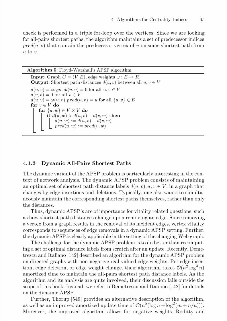
shall [568], Floyd [217] developed an APSP algorithm that achieves an O(n3)time bound, see Algorithm 5. The algorithm first initializes all distance labelsto infinity, and then sets the distance labels d(u, v), for u, v ∈ E , to the edgelengths ω(u, v). After this initialization, the algorithm basically checks whetherthere exists a vertex triple u,v,w for which the distance labels violate the condi-tion in Lemma 4.1.1. If so, it decreases the involved distance label d(u, w). This




check is performed in a triple for-loop over the vertices. Since we are lookingfor all-pairs shortest paths, the algorithm maintains a set of predecessor indices

pred(u, v) that contain the predecessor vertex of v on some shortest path fromu to v.

Algorithm 5: Floyd-Warshall’s APSP algorithm

Input: Graph G = (V, E ), edge weights ω : E → ROutput: Shortest path distances d(u, v) between all u, v ∈ V

d(u, v) = ∞,pred(u, v) = 0 for all u, v ∈ V d(v, v) = 0 for all v ∈ V d(u, v) = ω(u, v),pred(u, v) = u for all u, v ∈ E for v ∈ V do

for u, w ∈ V × V doif d(u, w) > d(u, v) + d(v, w) thend(u, w) := d(u, v) + d(v, w)

pred(u, w) := pred(v, w)

4.1.3 Dynamic All-Pairs Shortest Paths

The dynamic variant of the APSP problem is particularly interesting in the con-text of network analysis. The dynamic APSP problem consists of maintainingan optimal set of shortest path distance labels d(u, v), u , v ∈ V , in a graph thatchanges by edge insertions and deletions. Typically, one also wants to simulta-neously maintain the corresponding shortest paths themselves, rather than onlythe distances.

Thus, dynamic APSP’s are of importance for vitality related questions, suchas how shortest path distances change upon removing an edge. Since removing

a vertex from a graph results in the removal of its incident edges, vertex vitalitycorresponds to sequences of edge removals in a dynamic APSP setting. Further,the dynamic APSP is clearly applicable in the setting of the changing Web graph.

The challenge for the dynamic APSP problem is to do better than recomput-ing a set of optimal distance labels from scratch after an update. Recently, Deme-trescu and Italiano [142] described an algorithm for the dynamic APSP problemon directed graphs with non-negative real-valued edge weights. Per edge inser-tion, edge deletion, or edge weight change, their algorithm takes O(n2 log3 n)amortized time to maintain the all-pairs shortest path distance labels. As the

algorithm and its analysis are quite involved, their discussion falls outside thescope of this book. Instead, we refer to Demetrescu and Italiano [142] for detailson the dynamic APSP.

Further, Thorup [549] provides an alternative description of the algorithm,as well as an improved amortized update time of O(n2(log n +log2(m + n/n))).Moreover, the improved algorithm allows for negative weights. Roditty and



66 R. Jacob et al.

Zwick [496] argue that the dynamic SSSP problem on weighted graphs is asdifficult as the static APSP problem. Further, they present a randomized algo-rithm for the dynamic APSP, returning correct results with very high probability,with improved amortized update time for sparse graphs.

4.1.4 Maximum Flows and Minimum-Cost Flows

For flow betweenness (see Section 3.6.1), the maximum flow between a des-ignated source node s and a designated sink node t needs to be computed.The maximum-flow problem has been studied extensively in the literature, andseveral algorithms are available. Some are generally applicable, some focus onrestricted cases of the problem, such as unit edge capacities, and others pro-vide improvements that may have more theoretical than practical impact. The

same applies to minimum-cost flows, with the remark that minimum-cost flowalgorithms are even more complex.

Again, we refer to the textbooks by Ahuja, Magnanti, and Orlin [6], andCormen, Leiserson, Rivest, and Stein [133] for good in-depth descriptions of thealgorithms. To give an idea of flow algorithms’ worst-case running times, andof the resulting impact on centrality computations in large networks, we brieflymention the following algorithms. The preflow-push algorithm by Goldberg andTarjan [252] runs in O(nm log(n2/m)), and the capacity scaling algorithm byAhuja and Orlin [8] runs in O(nm log U ), where U is the largest edge capac-

ity. For minimum cost flows, the capacity scaling algorithm by Edmonds andKarp [172] runs in O((m log U )(m + n log n)).

Alternatively, both maximum flow and minimum-cost flow problems can besolved using linear programming. The linear program for flow problems has aspecial structure which guarantees an integer optimal solution for any integerinputs (costs, capacities, and net inflows). Moreover, specialized network simplexalgorithms for flow-based linear programs with polynomial running times areavailable.

4.1.5 Computing the Largest Eigenvector

Several centrality measures described in this part of the book are based on thecomputation of eigenvectors of a given matrix. This section provides a short in-troduction to the computation of eigenvectors and eigenvalues. In general, theproblem of computing eigenvalues and eigenvectors is non-trivial, and completebooks are dedicated to this topic. We focus on a single algorithm and sketchthe main idea. All further information, such as optimized algorithms, or algo-rithms for special matrices, are available in textbooks like [256, 482]. Further-

more, Section 14.2 (chapter on spectral analysis) considers the computation of all eigenvalues of the matrix representing a graph.

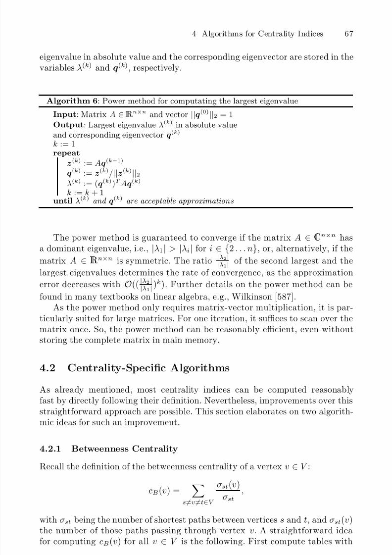
The eigenvalue with largest absolute value and the corresponding eigenvectorcan be computed by the power method, which is described by Algorithm 6. Asinput the algorithm takes the matrix A and a start vector q

(0) ∈Ê

n with||q(0)||2 = 1. After the k-th iteration, the current approximation of the largest




eigenvalue in absolute value and the corresponding eigenvector are stored in thevariables λ(k) and q

(k), respectively.

Algorithm 6: Power method for computating the largest eigenvalue

Input: Matrix A ∈ Ê

n×n and vector ||q(0)||2 = 1

Output: Largest eigenvalue λ(k) in absolute valueand corresponding eigenvector q(k)

k := 1repeat

z(k) := Aq(k−1)

q(k) := z

(k)/||z(k)||2λ(k) := (q(k))T Aq(k)

k := k + 1until λ(k) and q(k) are acceptable approximations

The power method is guaranteed to converge if the matrix A ∈

n×n hasa dominant eigenvalue, i.e., |λ1| > |λi| for i ∈ 2 . . . n, or, alternatively, if the

matrix A ∈Ê

n×n is symmetric. The ratio |λ2||λ1|

of the second largest and the

largest eigenvalues determines the rate of convergence, as the approximation

error decreases with O(( |λ2|

|λ1

|

)k). Further details on the power method can be

found in many textbooks on linear algebra, e.g., Wilkinson [587].As the power method only requires matrix-vector multiplication, it is par-

ticularly suited for large matrices. For one iteration, it suffices to scan over thematrix once. So, the power method can be reasonably efficient, even withoutstoring the complete matrix in main memory.

4.2 Centrality-Specific Algorithms

As already mentioned, most centrality indices can be computed reasonablyfast by directly following their definition. Nevertheless, improvements over thisstraightforward approach are possible. This section elaborates on two algorith-mic ideas for such an improvement.

4.2.1 Betweenness Centrality

Recall the definition of the betweenness centrality of a vertex v ∈ V :

cB(v) =

s=v=t∈V

σst(v)σst

,

with σst being the number of shortest paths between vertices s and t, and σst(v)the number of those paths passing through vertex v. A straightforward ideafor computing cB(v) for all v ∈ V is the following. First compute tables with



68 R. Jacob et al.

the length and number of shortest paths between all vertex pairs. Then, foreach vertex v, consider all possible pairs s and t, use the tables to identify thefraction of shortest s-t-paths through v, and sum these fractions to obtain thebetweenness centrality of v.

For computing the number of shortest paths in the first step, one can adjustDijkstra’s algorithm as follows. From Lemma 4.1.1, observe that a vertex v is on ashortest path between two vertices s and t if and only if d(s, t) = d(s, v)+ d(v, t).We replace the predecessor vertices by predecessor sets pred(s, v), and each timea vertex w ∈ N (v) is scanned for which d(s, t) = d(s, v) + d(v, t), that vertex isadded to the predecessor set pred(s, v). Then, the following relation holds:

σsv =

u∈ pred(s,v)

σsu.

Setting pred(s, v) = s for all v ∈ N (s), we can thus compute the number of shortest paths between a source vertex s and all other vertices. This adjustmentcan easily be incorporated into Dijkstra’s algorithm, as well as in the BFS forunweighted graphs.

As for the second step, vertex v is on a shortest s-t-path if d(s, t) = d(s, v) +d(v, t). If this is the case, the number of shortest s-t-paths using v is computedas σst(v) = σsv · σvt. Thus, computing cB(v) requires O(n2) time per vertex vbecause of the summation over all vertices s = v = t, yielding O(n3) time in

total. This second step dominates the computation of the length and the numberof shortest paths. Thus, the straightforward idea for computing betweennesscentrality has an overall running time of O(n3).

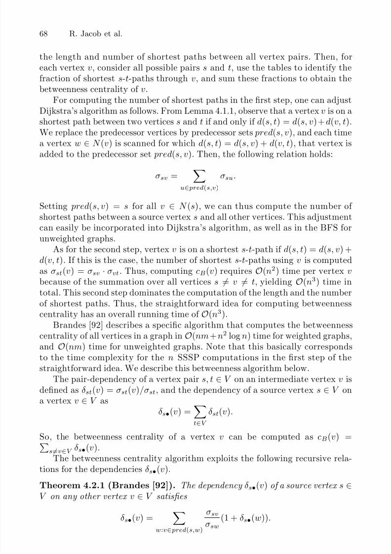
Brandes [92] describes a specific algorithm that computes the betweennesscentrality of all vertices in a graph in O(nm+ n2 log n) time for weighted graphs,and O(nm) time for unweighted graphs. Note that this basically correspondsto the time complexity for the n SSSP computations in the first step of thestraightforward idea. We describe this betweenness algorithm below.

The pair-dependency of a vertex pair s, t ∈ V on an intermediate vertex v is

defined as δst(v) = σst(v)/σst, and the dependency of a source vertex s ∈ V ona vertex v ∈ V as

δs•(v) =t∈V

δst(v).

So, the betweenness centrality of a vertex v can be computed as cB(v) =s=v∈V δs•(v).

The betweenness centrality algorithm exploits the following recursive rela-tions for the dependencies δs•(v).

Theorem 4.2.1 (Brandes [92]). The dependency δs•(v) of a source vertex s ∈V on any other vertex v ∈ V satisfies

δs•(v) =

w:v∈ pred(s,w)

σsv

σsw(1 + δs•(w)).




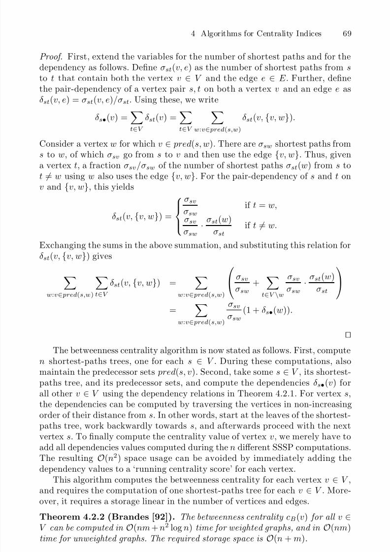
Proof. First, extend the variables for the number of shortest paths and for thedependency as follows. Define σst(v, e) as the number of shortest paths from sto t that contain both the vertex v ∈ V and the edge e ∈ E . Further, definethe pair-dependency of a vertex pair s, t on both a vertex v and an edge e as

δst(v, e) = σst(v, e)/σst. Using these, we write

δs•(v) =t∈V

δst(v) =t∈V

w:v∈ pred(s,w)

δst(v, v, w).

Consider a vertex w for which v ∈ pred(s, w). There are σsw shortest paths froms to w, of which σsv go from s to v and then use the edge v, w. Thus, givena vertex t, a fraction σsv/σsw of the number of shortest paths σst(w) from s tot = w using w also uses the edge v, w. For the pair-dependency of s and t onv and v, w, this yields

δst(v, v, w) =

σsv

σswif t = w,

σsv

σsw·

σst(w)

σstif t = w.

Exchanging the sums in the above summation, and substituting this relation forδst(v, v, w) gives

w:v∈ pred(s,w)

t∈V

δst(v, v, w) = w:v∈ pred(s,w)

σsv

σsw

+ t∈V \w

σsv

σsw

·σst(w)

σst

=

w:v∈ pred(s,w)

σsv

σsw(1 + δs•(w)).

The betweenness centrality algorithm is now stated as follows. First, computen shortest-paths trees, one for each s ∈ V . During these computations, alsomaintain the predecessor sets pred(s, v). Second, take some s ∈ V , its shortest-

paths tree, and its predecessor sets, and compute the dependencies δs•(v) forall other v ∈ V using the dependency relations in Theorem 4.2.1. For vertex s,the dependencies can be computed by traversing the vertices in non-increasingorder of their distance from s. In other words, start at the leaves of the shortest-paths tree, work backwardly towards s, and afterwards proceed with the nextvertex s. To finally compute the centrality value of vertex v, we merely have toadd all dependencies values computed during the n different SSSP computations.The resulting O(n2) space usage can be avoided by immediately adding thedependency values to a ‘running centrality score’ for each vertex.

This algorithm computes the betweenness centrality for each vertex v ∈ V ,and requires the computation of one shortest-paths tree for each v ∈ V . More-over, it requires a storage linear in the number of vertices and edges.

Theorem 4.2.2 (Brandes [92]). The betweenness centrality cB(v) for all v ∈V can be computed in O(nm + n2 log n) time for weighted graphs, and in O(nm)time for unweighted graphs. The required storage space is O(n + m).



70 R. Jacob et al.

Other shortest-path based centrality indices, such as closeness centrality,graph centrality, and stress centrality can be computed with similar shortest-paths tree computations followed by iterative dependency computations. Forfurther details on this, we refer to Brandes [92].

4.2.2 Shortcut Values

Another algorithmic task is to compute the shortcut value for all edges of adirected graph G = (V, E ), as introduced in Section 3.6.3. More precisely, thetask is to compute the shortest path distance from vertex u to vertex v inGe = (V, E \ e) for every directed edge e = (u, v) ∈ E . The shortcut value foredge e is a vitality based centrality measure for edges, defined as the maximumincrease in shortest path length (absolute, or relative for non-negative distances)

if e is removed from the graph.The shortcut values for all edges can be naıvely computed by m = |E | calls to

a SSSP routine. This section describes an algorithm that computes the shortcutvalues for all edges with only n = |V | calls to a routine that is asymptotically asefficient as a SSSP computation. To the best of our knowledge this is the firstdetailed exposition of this algorithm, which is based on an idea of Brandes.

We assume that the directed graph G contains no negative cycles, such thatd(i, j) is well defined for all vertices i and j. To simplify the description weassume that the graph contains no parallel edges, such that an edge is identified

by its endpoints.The main idea is to consider some vertex u, and to execute one computation

to determine the shortcut values for all edges starting at u. These shortcutvalues are defined by shortest paths that start at vertex u and reach an adjacentvertex v, without using the edge (u, v). To compute this, define αi = d(u, i)to be the length of a shortest path from u to i, the well known shortest pathdistance. Further, let the variable τ i ∈ V denote the second vertex (identifyingthe first edge of the path) of all paths from u to i with length αi, if this is unique,otherwise it is undefined, τ i = ⊥. Thus, τ i = ⊥ implies that there are at least

two paths of length αi from u to i that start with different edges. Finally, thevalue β i is the length of the shortest path from u to i that does not have τ i asthe second vertex, ∞ if no such path exists, or β i = αi if τ i = ⊥.

Assume that the values αv, τ v, and β v are computed for a neighbor v of u.Then, the shortcut value for the edge (u, v) is αv if τ v = v, i.e., the edge (u, v)is not the unique shortest path from u to v. Otherwise, if τ v = v, the value β v isthe shortcut value for (u, v). Hence, it remains to compute the values αi, τ i, β ifor i ∈ V . The algorithm exploits that the values αi, τ i, β i obey some recursions.At the base of these recursions we have:

αu = 0, τ u = ∅, β u = ∞

The values αj obey the shortest paths recursion:

αj = mini:(i,j)∈E

αi + ω(i, j)




To define the recursion for τ j , it is convenient to consider the set of incomingneighbors I j of vertices from which a shortest path can reach j,

I j = i | (i, j) ∈ E and αj = αi + ω(i, j) .

It holds that

τ j =

j if I j = u,

a if a = τ i for all i ∈ I j(all predecessors have first edge (u, a)),

⊥ otherwise.

The value τ j is only defined if all shortest paths to vertex j start with the sameedge, which is the case only if all τ i values agree on the vertices in I j . For thecase τ j = ⊥ it holds that β j = αj , otherwise

β j = min

min

i:(i,j)∈E,τ i=τ j

β i + ω(i, j) , mini:(i,j)∈E,τ i=τ j

αi + ω(i, j)

.

To see this, consider the path p that achieves β j , i.e., a shortest path p fromu to j that does not start with τ j . If the last vertex i of p before j has τ i = τ j ,the path p up to i does not start with τ j , and this path is considered in β i andhence in β j . If instead the path p has as the next to last vertex i, and τ i = τ j ,

then one of the shortest paths from u to i does not start with τ j , and the lengthof p is αi + ω(i, j).

With the above recursions, we can efficiently compute the values αi, τ i, β i.For the case of positive weights, any value αi depends only on values αj thatare smaller than αi, so these values can be computed in non-decreasing order(just as Dijkstra’s algorithm does). If all edge weights are positive, the directedgraph containing all shortest paths (another view on the sets I j) is acyclic, andthe values τ i can be in topological order. Otherwise, we have to identify thestrongly connected components of G, and contract them for the computation

of τ . Observe that β i only depends upon β j if β j ≤ β i. Hence, these valuescan be computed in non-decreasing order in a Dijkstra-like algorithm. In theunweighted case, this algorithm does not need a priority queue and its runningtime is only that of BFS.

If there are negative edge weights, but no negative cycles, the Dijkstra-like algorithm is replaced by a Bellman-Ford type algorithm to compute theα values. The computation of τ remains unchanged. Instead of computing β i,we compute β i = β i − αi, i.e., we apply the shortest-paths potential toavoid negative edge weights. This replaces all ω(i, j) terms with terms of the

form ω(i, j) − αj + αi ≥ 0, and hence the β i values can be set in increasing order,and this computes the β i values as well.

Note that the above method can be modified to also work in networks withparallel edges. There, the first edge of a path is no longer identified by thesecond vertex of the path, such that this edge should be used instead. We caneven modify the method to compute the shortcut value of the vertex v, i.e.,



72 R. Jacob et al.

the two neighbors of v whose distance increases most if v is deleted from thenetwork. To achieve this, negate the length and direction of the incoming edges,run the above algorithm, and subtract the length of the outgoing edges from theresulting β i values on the neighbors of v. In this way, for all pairs of neighbors

that can reach each other through v the difference between the direct connectionand the shortest alternative are computed.

Summarizing, we showed that in the above mentioned types of graphs allshortcut values can be computed in the time of computing n times a SSSP.

4.3 Fast Approximation

Most of the centralities introduced in Chapter 3 can be computed in polynomial

time. Although this is a general indication that such computations are feasible, itmight still be practically impossible to analyze huge networks in reasonable time.As an example, it may be impossible to compute betweenness centrality for largenetworks, even when using the improved betweenness algorithm of Section 4.2.1.This phenomenon is particularly prominent when investigating the web graph.For such a huge graph, we typically do not want to invest more than a smallnumber of scans over the complete input.

With this limited computational investment, it might not be possible to de-termine exact centrality values. Instead, the focus should be on approximate

solutions and their quality. In this setting, approximation algorithms provide aguaranteed compromise between running time and accuracy.

Below, we describe an approximation algorithm for the calculation of close-ness centrality, and then adapt this algorithm to an approximative calculationfor betweenness centrality. Next, Section 4.3.2 discusses approximation methodsfor the computation of web centralities.

4.3.1 Approximation of Centralities Based on All Pairs ShortestPaths Computations

We have argued above that the calculation of centrality indices can require alot of computing time. This also applies to the computation of all-pairs shortestpaths, even when using the algorithms discussed in Section 4.1.2. In many ap-plications, it is valuable to instead compute a good approximate value for thecentrality index, if this is faster. With the random sampling technique intro-duced by Eppstein and Wang [179], the closeness centrality of all vertices in aweighted, undirected graph can be approximated in O( log n

2 (n log n + m)) time.The approximated value has an additive error of at most ∆G with high proba-

bility, where is any fixed constant, and ∆G is the diameter of the graph. Weadapt this technique for the approximative calculation of betweenness central-ity, yielding an approximation of the betweenness centrality of all vertices in aweighted, directed graph with an additive error of (n − 2), and with the sametime bound as above.




The following randomized approximative algorithm estimates the closenesscentrality of all vertices in a weighted graph by picking K sample vertices andcomputing single source shortest paths (SSSP) from each sample vertex to allother vertices. Recall the definition of closeness centrality of a vertex v ∈ V :

cC (v) =

x∈V

d(v, x)

n − 1. (4.1)

The centrality cC (v) can be estimated by the calculation of the distance of v toK other vertices v1, . . . , vK as follows

cC (v) =n

K · (n − 1)

K

i=1

d(v, vi). (4.2)

For undirected graphs, this calculates the average distance from v to K othervertices, then scales this to the sum of distances to/from all other n vertices,and divides by n − 1. As both cC and cC consider average distances in the graph,the expected value of cC (v) is equal to cC (v) for any K and v. This leads to thefollowing algorithm:

1. Pick a set of K vertices v1, v2, . . . , vK uniformly at random from V .2. For each vertex v ∈ v1, v2, . . . , vK, solve the SSSP problem with that

vertex as source.

3. For each vertex v ∈ V , compute cC (v) =n

K · (n − 1)

Ki=1

d(v, vi)

We now recapitulate the result from [179] to compute the required number of sample vertices K that suffices to achieve the desired approximation. The resultuses Hoeffding’s Bound [299]:

Lemma 4.3.1. If x1, x2, . . . , xK are independent with ai ≤ xi ≤ bi, and µ =

E [

xi/K ] is the expected mean, then for ξ > 0

Pr

K

i=1 xi

K − µ

≥ ξ

≤ 2 · e−2K2ξ2/

È Ki=1(bi−ai)2 . (4.3)

By setting xi to n·d(vi,u)n−1

, µ to cC (v), ai to 0, and bi to n∆n−1

, we can boundthe probability that the error of estimating cC (v) by cC (v), for any vertex, ismore than ξ:

Pr

K

i=1 xi

K − µ

≥ ξ

≤ 2 · e−2K2ξ2/

È Ki=1(bi−ai)2 (4.4)

= 2 · e−2K2ξ2/K( n∆n−1 )2 (4.5)

= 2 · e−Ω(Kξ2/∆2) (4.6)



74 R. Jacob et al.

If we set ξ to · ∆ and use Θ( log n2 ) samples, the probability of having an

error greater than · ∆ is at most 1/n for every estimated value.The running time of an SSSP algorithm is O(n + m) in unweighted graphs,

and O(m + n log n) in weighted graphs, yielding a total running time of O(K ·

(n + m)) and O(K (m + n log n)) for this approach, respectively. With K setto Θ( log n

2 ), this results in running times of O( log n2 (n + m)) and O( log n

2 (m +n log n)).

We now adapt this technique to the estimation of betweenness centrality inweighted and directed graphs. As before, a set of K sample vertices is randomlypicked from V . For every source vertex vi, we calculate the total dependencyδvi•(v) (see Section 3.4.2) for all other vertices v, and sum them up. The esti-mated betweenness centrality cB(v) is then defined as

cB(v) =Ki=1

nK

δvi•(v). (4.7)

Again, the expected value of cB(v) is equal to cB(v) for all K and v. For thisnew problem, we set xi to n · δvi•, µ to cB(v), and ai to 0. The total dependencyδvi•(v) can be at most n − 2 if and only if v is the only responsible vertexfor all shortest paths leaving vi. Thus, we set bi to n(n − 2). Using the bound(4.3.1), it follows that the probability that the difference between the estimatedbetweenness centrality cB(v) and the betweenness centrality cB(v) is more than

ξ is

Pr |cB(v) − cB(v)| ≥ ξ ≤ 2e−2K2ξ2/K·(n(n−2))2 (4.8)

= 2 · e−2Kξ2/(n(n−2))2 (4.9)

Setting ξ to (n(n − 2)), and the number of sample vertices K to Θ(log n/2),the difference between the estimated centrality value and the correct value is atmost n(n − 1) with probability 1/n. As stated above, the total dependencyδvi•(v) of a vertex vi can be calculated in O(n + m) in unweighted graphs andin O(m + n log n) in weighted graph. With K set as above, this yields runningtimes of O( log n

2 (n + m)) and O( log n2 (m + n log n)), respectively. Hence, the

improvement over the exact betweenness algorithm in Section 4.2.1 is the factorK which replaces a factor n, for the number of SSSP-like computations.

Note that this approach can be applied to many centrality indices, namelythose that are based on summations over some primitive term defined for eachvertex. As such, those indices can be understood as taking a normalized average,which makes them susceptible to random vertex sampling.

4.3.2 Approximation of Web CentralitiesMost of the approximation and acceleration techniques for computing Web-centralities are designed for the PageRank method. Therefore, in the followingwe concentrate on this method. A good short overview of existing accelerationPageRank techniques can be found in [378]. We distinguish the following accel-eration approaches:




– approximation by cheaper computations, usually by avoiding matrix multipli-cations,

– acceleration of convergence,– solving a linear system of equations instead of solving an eigenvector problem,

– using decomposition of the Web-graph, and– updating instead of recomputations.

We discuss these approaches separately below.

Approximation by Cheaper Computations. In [148] and [149], Ding et al.report on experimental results indicating that the rankings obtained by bothPageRank and Hubs & Authorities are strongly correlated to the in-degree of the vertices. This especially applies if only the top-20 query results are taken into

consideration. Within the unifying framework the authors propose, the rankingby in-degree can be viewed as an intermediate between the rankings produced byPageRank and Hubs & Authorities. This result is claimed to also theoreticallyshow that the in-degree is a good approximation of both PageRank and Hubs &Authorities. This seems to be true for graphs in which the rankings of PageRankand Hubs & Authorities are strongly related. However, other authors performedcomputational experiments with parts of the Web graph, and detected only littlecorrelation between in-degree and PageRank, see, e.g., [463]. A larger scale studyconfirming the latter result can be found in [380].

Acceleration of Convergence. The basis for this acceleration technique isthe power method for determining the eigenvector corresponding to the largesteigenvalue, see Section 4.1.5.

Since each iteration of the power-method consists of matrix multiplication,and is hence very expensive for the Web graph, the goal is to reduce the numberof iterations. One possibility was proposed by Kamvar et al. [340] and extendedby Haveliwala et al. [292]. In the first paper the authors propose a quadratic

extrapolation that is based on the so-called Aitken ∆2

method. The Aitken ex-trapolation assumes that an iteratex(k−2) can be written as a linear combinationof the first two eigenvectors u and v. With this assumption, the next two iteratesare linear combinations of the first two eigenvectors as well:

x(k−2) = u + αv

x(k−1) = Ax(k−2) = u + αλ2v

x(k) = Ax(k−1) = u + αλ2

2v.

By defining

yi =

x

(k−1)i − x

(k−2)i

2

x(k)i − 2x

(k−1)i + x

(k−2)i

and some algebraic reductions (see [340]) we get y = αv and hence



76 R. Jacob et al.

u = x(k−2) − y. (4.10)

Note that the assumption that x(k−2) can be written as a linear combination of u and v is only an approximation, hence (4.10) is also only an approximation

of the first eigenvector, which is then periodically computed during the ordinarypower method.

For the quadratic extrapolation the authors assume that an iterate x(k−2)

is a linear combination of the first three eigenvectors u, v and w. Using thecharacteristic polynomial they arrive at an approximation of u only dependingon the iterates:

u = β 2x(k−2) + β 1x

(k−1) + β 0x(k).

As in the Aitken extrapolation, this approximation is periodically computedduring the ordinary power method. The authors report on computational ex-periments indicating that the accelerated power method is much faster than theordinary power method, especially for large values of the damping factor d, forwhich the power method converges very slowly. As we discuss in Section 5.5.2,this is due to the fact that d equals the second largest eigenvalue (see [290]),hence a large value for d implies a small eigengap.

The second paper [292] is based on the ideas described above. Instead of having a linear combination of only two or three eigenvector approximations, theauthors assume that x(k−h) is a linear combination of the first h + 1 eigenvectorapproximations. Since the corresponding eigenvalues are assumed to be the h-throots of unity, scaled by d, it is possible to find a simple closed form for the firsteigenvector. This acceleration step is used as above.

Kamvar et al. [338] presented a further idea to accelerate the convergence,based on the observation that the speed of convergence in general varies consid-erably from vertex to vertex. As soon as a certain convergence criteria is reachedfor a certain vertex, this vertex is taken out of the computation. This reduces thesize of the matrix from step to step and therefore accelerates the power method.

The Linear System Approach. Each eigenvalue problem

Ax = λx

can be written as homogeneous linear system of equations

(A − λI )x = 0n.

Arasu et al. [33] applied this idea to the PageRank algorithm and conductedsome experiments with the largest strongly connected component of a snapshot

of the Web graph from 1998. The most simple linear system approach for thePageRank system(I − dP ) cPR = (1 − d) 1n

is probably the Jacobi iteration. But, as was mentioned in the description of thePageRank algorithm, the Jacobi iteration is very similar to the power method,and hence does not yield any acceleration.




Arasu et al. applied the Gauss-Seidel iteration defined by

c(k+1)PR (i) = (1 − d) + d

j<i

pijc(k+1)PR ( j) + d

j>i

pijc(k)PR( j).

For d = 0.9, their experiments on the above described graph are very promising:the Gauss-Seidel iteration converges much faster than the power iteration. Arasuet al. then combine this result with the fact that the Web graph has a so-calledbow tie structure. The next paragraph describes how this structure and otherdecomposition approaches may be used to accelerate the computations.

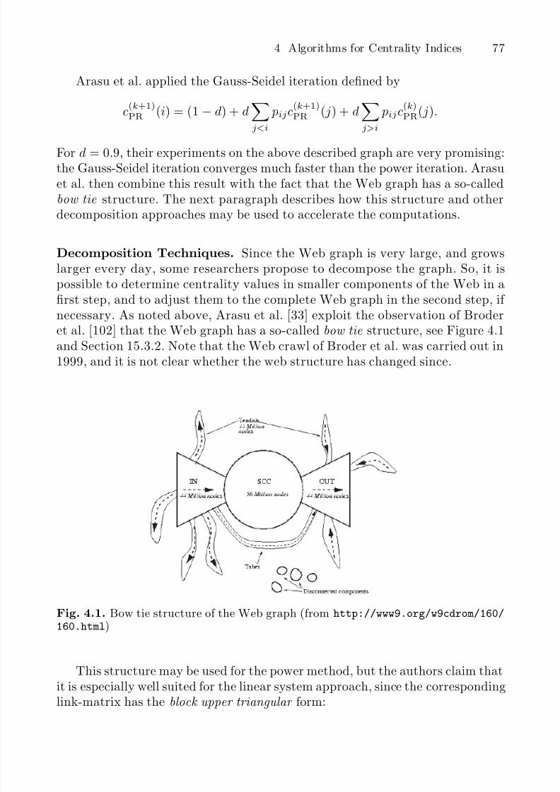
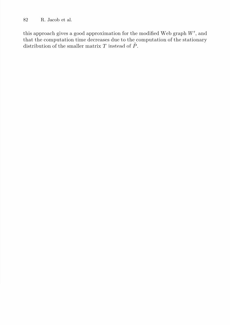
Decomposition Techniques. Since the Web graph is very large, and growslarger every day, some researchers propose to decompose the graph. So, it ispossible to determine centrality values in smaller components of the Web in afirst step, and to adjust them to the complete Web graph in the second step, if necessary. As noted above, Arasu et al. [33] exploit the observation of Broderet al. [102] that the Web graph has a so-called bow tie structure, see Figure 4.1and Section 15.3.2. Note that the Web crawl of Broder et al. was carried out in1999, and it is not clear whether the web structure has changed since.

Fig. 4.1. Bow tie structure of the Web graph (from http://www9.org/w9cdrom/160/160.html)

This structure may be used for the power method, but the authors claim thatit is especially well suited for the linear system approach, since the correspondinglink-matrix has the block upper triangular form:



78 R. Jacob et al.

P =

P 11 P 12 P 13 . . . P 1K0 P 22 P 23 . . . P 2K...

. . . P 33 . . . P 3K

... . . . . . . ...0 . . . . . . 0 P KK

.

By partitioning cPR in the same way, the large problem may be solved by thefollowing sequence of smaller problems

(I − dP KK ) cPR,K = (1 − d)1nK

(I − dP ii) cPR,i = (1 − d)1ni + dK

j=i+1

P ijcPR,j

A second approach was proposed by Kamvar et al. [339]. They investigated,besides a smaller partial Web graph, a Web crawl of 2001, and found the followinginteresting structure:

1. There is a block structure of the Web.2. The individual blocks are much smaller than the entire Web.3. There are nested blocks corresponding to domains, hosts and sub-

directories within the path.

Algorithm 7: PageRank exploiting the block structure: BlockRank

1. For each block I ,compute the local PageRank scores cPR(I)(i) for each vertex i ∈ I

2. Weight the local PageRank scoresaccording to the importance of the block the vertices belongs to

3. Apply the standard PageRank algorithmusing the vector obtained in the first two steps

Based on this observation, the authors suggest the three-step-algorithm 7. Inthe first and third step the ordinary PageRank algorithm can be applied. Thequestion is how to formalize the second step. This is done via a block graph Bwhere each block I is represented by a vertex, and an edge (I, J ) is part of theblock graph if there exists an edge (i, j) in the original graph satisfying i ∈ I and j ∈ J , where (i, j) may be a loop. The weight ωIJ associated with an edge

(I, J ) is computed as the sum of edge weights from vertices i ∈ I to j ∈ J in theoriginal graph, weighted by the local PageRank scores computed from Step 1:

ωIJ =

i∈I,j∈J

aijcPR(I)(i).




If the local PageRank vectors are normalized using the 1-norm, then theweight matrix Ω = (ωIJ ) is a stochastic matrix, and the ordinary PageRankalgorithm can be applied to the block graph B to obtain the block weights bI .

The starting vector for Step 3 is then determined by

c(0)PR(i) = cPR(I)(i)bI ∀ I, ∀ i ∈ I.

Another decomposition idea was proposed by Avrachenkov and Litvak [367]who showed that if a graph consists of several connected components (whichis obviously true for the Web graph), then the final PageRank vector may becomputed by determining the PageRank vectors in the connected componentsand combining them appropriately using the following theorem.

Theorem 4.3.2.

cPR =

|V 1||V |

cPR(1), |V 2||V |

cPR(2), . . . , |V K ||V |

cPR(K),

,

where Gk = (V k, E k) are the connected components, k = 1, . . . , K and cPR(k) is

the PageRank vector computed for the kth connected component.

Finally, we briefly mention the 2-step-algorithm of Lee et al. [383] that isbased on the observation that the Markov chain associated with the PageRankmatrix is lumpable.

Definition 4.3.3. If L = L1, L2, . . . , LK is a partition of the states of a Markov chain P then P is lumpable with respect to L if and only if for any

pair of sets L, L ∈ L and any state i in L the probability of going from i to L

doesn’t depend on i, i.e. for all i, i ∈ L

Pr[X t+1 ∈ L|X t = i] =j∈L

pij = Pr[X t+1 ∈ L|X t = i] =j∈L

pij .

The common probabilities define a new Markov chain, the lumped chain P L with

state space L and transition probabilities pLL = Pr[X t+1 ∈ L|X t ∈ L].

The partition the authors use is to combine the dangling vertices (i.e., ver-tices without outgoing edges) into one block and to take all dangling verticesas singleton-blocks. This is useful since the number of dangling vertices is of-ten much larger than the number of non-dangling vertices (a Web crawl from2001 contained 290 million pages in total, but only 70 million non-dangling ver-tices, see [339]). In a second step, the Markov chain is transformed into a chainwith all non-dangling vertices combined into one block using a state aggregationtechnique.

For the lumped chain of the first step, the PageRank algorithm is used for

computing the corresponding centrality values. For the second Markov chain,having all non-dangling vertices combined, the authors prove that the algorithmto compute the limiting distribution consists of only three iterations (and oneAitken extrapolation step, if necessary, see Section 4.3.2). The vectors obtainedin the two steps are finally concatenated to form the PageRank score vector of the original problem.



80 R. Jacob et al.

4.4 Dynamic Computation

In Section 4.3.2, several approaches for accelerating the calculation of page im-portance were described. In this section, we focus on the ‘on the fly’ computation

of the same information, and on the problem of keeping the centrality values up-to-date in the dynamically changing Web.

4.4.1 Continuously Updated Approximations of PageRank

For the computation of page importance, e.g. via PageRank, the link matrix hasto be known in advance. Usually, this matrix is created by a crawling process.As this process takes a considerable amount of time, approaches for the ‘on thefly’ computation of page importance are of interest. Abiteboul et al. [1] describe

the ‘On-line Page Importance Computation’ (OPIC) algorithm, which computesan approximation of PageRank, and does not require to store the possibly hugelink matrix.

The idea is based on the distribution of ‘cash.’ At initialization, every pagereceives an amount of cash and distributes this cash during the iterative compu-tation. The estimated PageRank can then be computed directly from the currentcash distribution, even while the approximation algorithm is still running.

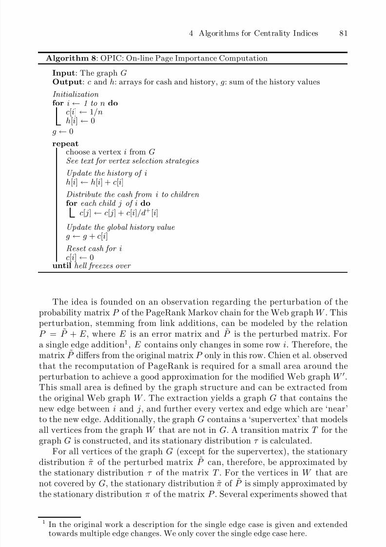
Algorithm 8 describes the OPIC algorithm. The array c holds the actualdistribution of cash for every page, and the array h holds the history of the cash

for every page. The scalar g is just a shortcut for

ni=1 h[i].An estimate of the PageRank of page i is given by cPRapprox(i) = h[i]+c[i]

g+1. To

guarantee that the algorithm calculates a correct approximation of PageRank,the selection of the vertices is crucial. Abiteboul et al. discuss three strategies:random, greedy, and circular. The strategies ‘randomly select a page’ and ‘cir-cularly select all pages’ are obvious. Greedy selects the page with the highestcash. For the convergence of the computation, the selection of the vertices hasto be fair, and this has to be guaranteed in all selection strategies.

After several iterations the algorithm converges towards the page impor-tance information defined by the eigenvector for the largest eigenvalue of theadjacency matrix of the graph. To guarantee the convergence of the calculationsimilar concepts as for the random surfer (see Section 3.9.3) have to be applied.These are, for example, the inclusion of a ‘virtual page’ that every page linksupon. The original work contains an adaptive version that covers link additionsand removals, and in some parts vertex additions and removals. This modifiedadaptive OPIC algorithm is not discussed here, and can be found in [1].

4.4.2 Dynamically Updating PageRankAn interesting approach to accelerate the calculation of page importance liesin the recomputation of the PageRank for the ‘changed’ part of the networkonly. In case of the Web these changes are page additions and removals and linkadditions and removals. For this idea, Chien et al. [124] described an approachfor link additions.




Algorithm 8: OPIC: On-line Page Importance Computation

Input: The graph GOutput: c and h: arrays for cash and history, g: sum of the history values

Initialization for i ← 1 to n do

c[i] ← 1/nh[i] ← 0

g ← 0

repeatchoose a vertex i from GSee text for vertex selection strategies

Update the history of ih[i] ← h[i] + c[i]

Distribute the cash from i to children for each child j of i do

c[ j] ← c[ j] + c[i]/d+[i]

Update the global history valueg ← g + c[i]

Reset cash for ic[i] ← 0

until hell freezes over

The idea is founded on an observation regarding the perturbation of theprobability matrix P of the PageRank Markov chain for the Web graph W . Thisperturbation, stemming from link additions, can be modeled by the relationP = P + E , where E is an error matrix and P is the perturbed matrix. Fora single edge addition1, E contains only changes in some row i. Therefore, thematrix P differs from the original matrix P only in this row. Chien et al. observedthat the recomputation of PageRank is required for a small area around theperturbation to achieve a good approximation for the modified Web graph W .This small area is defined by the graph structure and can be extracted fromthe original Web graph W . The extraction yields a graph G that contains thenew edge between i and j, and further every vertex and edge which are ‘near’to the new edge. Additionally, the graph G contains a ‘supervertex’ that modelsall vertices from the graph W that are not in G. A transition matrix T for thegraph G is constructed, and its stationary distribution τ is calculated.

For all vertices of the graph G (except for the supervertex), the stationarydistribution π of the perturbed matrix P can, therefore, be approximated bythe stationary distribution τ of the matrix T . For the vertices in W that arenot covered by G, the stationary distribution π of P is simply approximated bythe stationary distribution π of the matrix P . Several experiments showed that

1 In the original work a description for the single edge case is given and extendedtowards multiple edge changes. We only cover the single edge case here.



82 R. Jacob et al.

this approach gives a good approximation for the modified Web graph W , andthat the computation time decreases due to the computation of the stationarydistribution of the smaller matrix T instead of P .

05 algorithms for centrality indices

Documents