1

The Changing Effects of Oil Price Changes on Inflation

Adviser: Professor Bwo-Nung Huang

Professor Chin-Wei Yang

Advisee: Bi-Juan Lee

Abstract

This paper segments monthly data into three periods based on historical oil events. The

central purpose is to examine the relationship between real oil price changes and the inflation rates

in the framework of Mork’s (1989) asymmetrical model. We find: (1) a majority of countries

support long-run asymmetric responses of inflation rates to real oil price increases and decreases,

but they are nearly in linear relation in the three shorter periods; (2) the immediate responses of

inflation to real oil price changes are mainly larger than that of lagged periods, and the cumulative

impact of real oil price increase is in general larger than the cumulative impact of real oil price

decrease; (3) the direction of causality from real oil price changes to the inflation is nearly

unmistakable in both asymmetrical and linear cases, and it is particularly significant in a

cointegration relationship; and (4) the responses of inflation rates to oil price changes are generally

higher in Period I (pre-1986:12) than in Period II (1987:01-1998:12) or in Period III (post-1999:01),

which is in accord with actual observation.

2

1. Introduction

What is the relationship between oil prices and inflation? The price of oil and inflation are

often seen as being connected within a cause and effect framework. As oil prices move up or down,

inflation follows in the same direction. The reason why this happens may be that oil is a major input

in the economy - it is used in critical activities such as fueling transportation or goods made with

petroleum products - and if the costs of intermediate input rise, so should the cost of end output. For

instance, if the price of oil rises, then it will cost more to make plastic, and a plastics company will

then pass on some or all of this cost to the consumer, which raises prices and thus inflation.

With respect to the role of oil price changes in the economy, more and more studies show that

there is a nonlinear relationship between oil prices and economic variables. Nearly all of the

empirical analyses after Mork’s (1989) study have found asymmetric economic responses to oil

price changes. The asymmetry question has influenced much of the research such as Mork et al.

(1994), Hamilton (1996), Cuñado and Pérez de Gracia (2005), and so on. They find that no

significant relationship exists between oil-economy by using only oil price change as variable. Thus,

all studies after 1990 began to include a separate negative and positive oil price changes variables as

an alternative specification. To this end, the technique of entering both negative and positive real oil

price changes is used to perform the asymmetrical transmission in this paper.

To provide a further insight, according to the historical statistics, the direct relationship

between oil price and inflation was evident in the 1970s, when the cost of oil rose from a nominal

price of $3 before the 1973 oil crisis to close $40 during the 1979 oil crisis. This helped cause the

consumer price index (CPI), a key measure of inflation, to more than double from 41.101 in

January 1972 to 86.30 by the end of 1980. However, this relationship between oil and inflation

started to deteriorate after the 1980s. During the 1990's Gulf War (oil crisis), crude prices doubled

in six months from around $20 to around $40, but CPI remained relatively stable, growing from

134.6 in January 1991 to 137.9 in December 1991. In this relationship, it is even more noticeable

1 The Consumer Price Index (CPI) is compiled by the Bureau of Labor Statistics. Consumer Price Index is based upon 1982 (base of 100). For example, the CPI of 158 indicates 58% inflation since 1982. The commonly quoted inflation rate of say 3% is actually the change in the Consumer Price Index from a year earlier.

3

during the oil price hike from 1999 to 2008, in which the monthly average nominal price of oil

started rising from the recent low point ($11.32) in January 1999 to $109.05 in April 2008. During

this same period, the CPI rose from 164.30 in January 1999 to 214.82 in April 2008.

Judging by the data, obviously, it seems that the strong correlation between oil prices and

inflation contains some degree of nonlinearity, which is consistent with prior research mentioned

above. As a matter of fact, the effects of oil price changes on inflation rates may be comparatively

tiny in the long run, but they could be significant over relatively short periods, i.e., Huntington

(2005). Most importantly, the effects of a given change in the price of oil may vary over time. In

order to capture the more accurate transmission of oil price changes to CPI inflation, we partition

our whole sample into three independent periods according to the important historical events. The

first period spans before December 1986, a period characterized by oil supply shocks; the second

period spans from January 1987 to December 1998, a period of relative stability for oil prices; and

the third spans from January 1999 to the present, a period characterized by frequent run-up oil

prices.

Moreover, the advantage of splitting our sample is that it allows the elasticity of inflation with

respect to oil price change to vary at different periods and would give a more precise assessment of

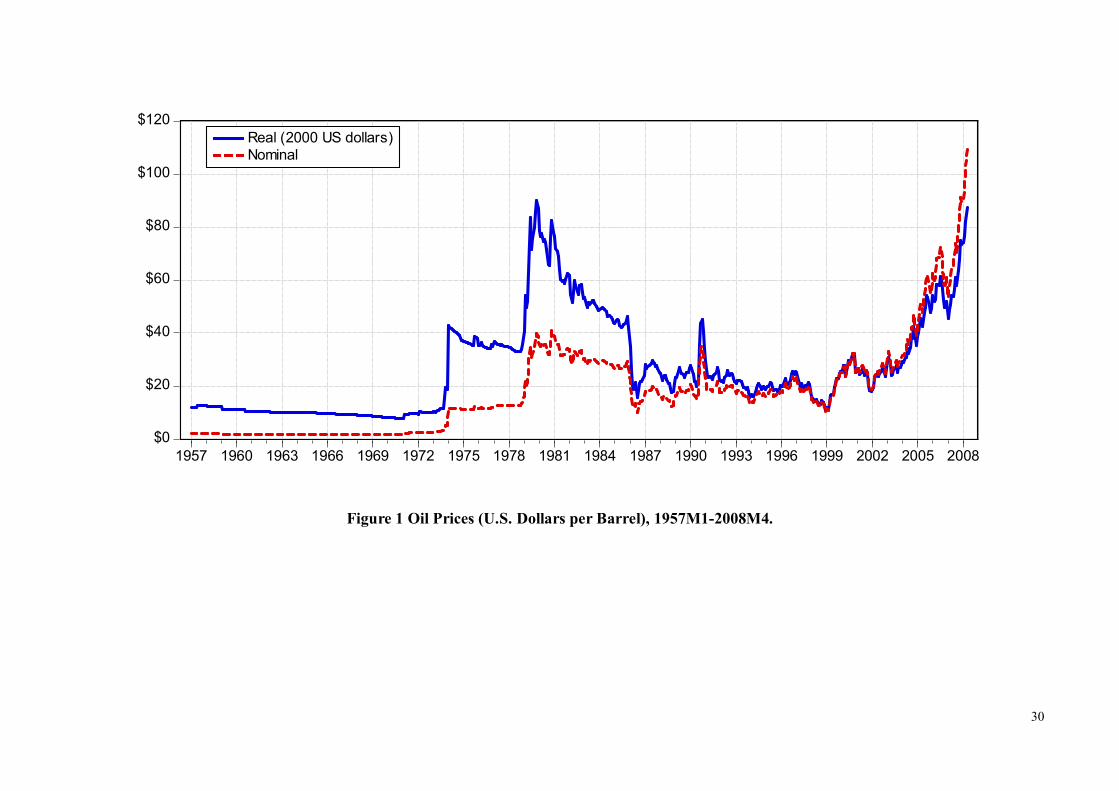
the oil pass-through parameter. The pattern of oil prices is shown in Figure 1. Real oil price plotted

by the solid line is adjusted for inflation, and the dotted line is nominal oil price measured by

current U.S. dollars. Note that the oil prices displayed substantial changes over the period, with two

major price increases occurring in the late 1973 and 1979, a major fall in 1986, a major price spike

around the Gulf War in 1990, and a considerable rise from 1999 to 2008.

The purpose of this paper is to investigate the oil price-CPI inflation relationship by means of

applying Mork’s (1989) asymmetrical model using monthly data. To the best of our knowledge, the

analysis in this paper departs from the existing literature in several respects. First, we divide our

whole data period into three subsamples by essential events in the world oil market; this allows the

oil price transmission to be different over time. Moreover, it helps us to have an insight into the

influence of oil price shock on inflation across different eras. Second, we employ an advanced

4

methodology in examining the effect of inflation with respect to oil price shocks, which are further

separated into oil price increase and oil price decrease. Much more reasonable than the previous

papers, we do not enter positive and negative oil price change as separate variables into estimated

equation arbitrarily. Rather, the separate value is derived from the parameter stability test results.

Specifically, we can inspect the response of inflation using positive and negative oil price change as

threshold or just take a simply oil price change in different individual country at different

sub-period. Finally, a majority of the earlier empirical studies have focused on the effects of oil

shocks on real output, however, in this paper we put the emphasis on the responses of inflation to

oil price change. This is also an important issue for economists and policy makers because oil prices

and inflation are very closely correlated with the growing global economy at the present time.

By using time-series data for oil prices, consumer price indexes, exchange rates, and interest

rates, this paper analyzes the influence of oil price change on inflation. We formally examine three

related questions. First, do oil price changes generate inflation? If so, how does inflation respond?

And what is the magnitude of the response? Second, does the asymmetric response behavior exist in

the sample period? If so, does the impact of oil price increase on the level of inflation rate differs

from that of oil price decrease? Third, are responses of inflation to oil price shocks similar among

countries across three periods? We answer these questions by exploring the shock of oil prices on

inflation in 29 countries, including Austria, Belgium, Canada, Chile, Colombia, Côte d’Ivoire,

Denmark, Finland, France, Germany, India, Italy, Japan, Korea, Luxembourg, Malaysia, Mexico,

Netherlands, Nigeria, Norway, Portugal, South Africa, Spain, Sweden, Trinidad and Tobago, the

United Kingdom, the United States, Venezuela, and Taiwan.

This paper is organized as follows. Next section, Section 2 provides a review of the related

literature. Section 3 introduces the empirical models. Section 4 describes the data and some

preliminary tests: unit root, cointegration, and the parameter instability tests before an adequate

model is used to estimate the relationship between real oil prices and inflation for each country in

each period. The final section, Section 5, provides concluding remarks and some policy

implications derived from this research.

5

2. Literature Review

A large body of empirical research has confirmed that oil price increases have strong and

negative influences for the real economy (e.g., Hamilton, 1983; Burbidge and Harrison, 1984;

Gisser and Goodwin, 1986; and Cuñado and Pérez de Gracia, 2003). Since the rapid fall of oil price

in 1986, the established model has been challenged. There was little evidence to suggest that oil

price decreases improve economic activity, in the same way that oil price increases suppress

economic activity. Several authors therefore reexamined the oil price-macroeconomic relationship,

using instead asymmetric or nonlinear methods (i.e., Mork, 1989; Mork et al., 1994; Lee et al., 1995;

Hamilton, 1996; Hamilton, 2003; and Cuñado and Pérez de Gracia, 2005). They found that the

negative linkage between oil price increases and economic activity still held. Consequently, it may

be reasonable to partition oil price changes into oil price increases and decreases for the analysis of

the related issue.

Although a considerable amount of research has found that oil price shocks have affected the

real output, only a few emphasize the effects of inflation. Quite recently, Blanchard and Galí (2007)

examined the effects of the recent oil shock on output and inflation and attempted to answer why

the current shocks (as in the 2000s) have had smaller effects on output and inflation than that in the

1970s. De Gregorio et al. (2007) provided a variety of estimates of the degree of transmission from

oil prices to inflation over time for a large set of countries. Moreover, using a structural cointegrated

VAR model for G-7 countries, Cologini and Manera (2008) found that for all countries except Japan

and U.K., changes in oil prices did influence the inflation rates.

In addition, some researchers suggested that oil price shocks on real GDP growth or CPI were

comparatively small on average, but that they did matter in particular time period. For example,

Bernanke et al. (1997) estimated their model over the whole sample and over each of the three

decades (1966-75, 1976-85, and 1986-1995); Kilian (2008) focused on five specific oil shock

episodes: 1973/74, 1978, 1980, 1990/91, and 2002/03, respectively. However, some problems may

arise from these two studies. In the paper by Bernanke et al., the division of ten years as a

subsample is arbitrary. In the Kilian paper, on the other hand, the estimates may be sensitive to the

6

choice of sample and as such may lead to potential bias due to inadequate observations. To

circumvent these problems, we split our sample into three sub-periods according to the well-known

historical events. This way, the ensuing results may better capture the mechanism of oil price

transmission and evaluate it more accurately.

3. Methodology

Following Hamilton (1996) and Hooker (1999), we use the world price of crude oil in real

terms deflated by consumer price indexes as a proxy for real oil prices. Moreover, world inflation

and oil prices were highly correlated during the last four decade as was indicated in Krichene

(2006). Thus we use the log difference of consumer price index as a key measure of inflation rates.

If only two variables are included to analyze the impact of oil prices on consumer price indexes, the

estimated results might be biased due to the possibility that an oil price change can affect other

economic variables such as interest rates and exchange rates as well.

Since the monetary policy is the primary tool to prevent inflation. Central banks may

fine-tune inflation to a significant extent through targeting interest rates. On the other hand,

previous papers have found that interest rate was an important factor to be included in the

discussion of the oil price-GDP relationship such as Huang et al. (2005) and Huang (2008). For this

reason, we choose the interest rates as one of our control variables in the model. Moreover,

exchange rate has been largely omitted from the related literature, thus the inclusion of this variable

seems appropriate because it surely play a major role in monetary policy in the international

economy as pointed out by Krugman (1983) and Rogoff (1991). Accordingly, it is also necessary to

take exchange rate into account. As such, the study on the response of inflation from oil price

changes should include oil price change ( tlroilp ), inflation rate ( tlcpi ), interest rate change ( tr ),

and exchange rate change ( ter ).

Due to the possibility of asymmetric response of inflation from oil price change, it is

necessary to take into account the asymmetry to improve the model. The asymmetrical relationship

between oil price shocks and an economy is investigated in many papers such as Mork (1989),

7

Hamilton (1996), Hooker (1999), Cuñado and Pérez de Gracia (2005), and so forth. As discussed in

these studies, the oil price-GDP relationship is sensitive to model specification and empirical data

period (i.e. including oil price volatility of 1980s, 1990s, and later). No significant relationship

exists between oil price-GDP by using only oil price change variable. As a result, all researches

after the 1990s start to include separate positive and negative oil price change variables.

However, issues can be raised on the prior papers that used an arbitrary asymmetrical model

to allow for a separate positive and negative oil price changes without first assessing parameter

stability tests of the involved variable. Hence, we utilize Hansen’s (1992) parameter stability tests to

perform the asymmetry test. In the case of unstable oil price change parameters, we enter real oil

price increases and decreases as separate variables in the equation. Conversely, a simple oil price

change variable will be taken in estimated equation when the result of stable oil price change

parameters is ascertained.

Given the background, the model can be specified as follows. The dependent variable of the

model is the log change in CPI, and all the explanatory variables are lagged. Apart from the log

change of CPI and oil price variables, there are interest rate change and exchange rate change. In

absent of long-run equilibrium among the variables and with the presence of asymmetrical

transmission from oil prices to inflation rates, we present the following model

t

p

iiti

p

i

p

iitiiti

p

iiti

p

iitit lcpierrlroilplroilplcpi

11 100

(1)

where tlroilp and tlroilp are respectively real oil price increases and real oil price decreases,

lcpi , lroilp , r ,and er represent respectively the difference of consumer price index and real

oil price (after logarithm) as well as the difference of interest rates and exchange rates. The

residual, t , is assumed to be independently and identically distributed with N(0,1). The optimal lag

length in the model is chosen by minimizing the Akaike information criterion (AIC). Note that we

include the current variable of oil price changes in the right hand side because it would help us to

capture its current impact on inflation rates.

For countries exist neither cointegration relationship among the variables nor asymmetrical

8

responses of inflation from oil price changes, equation (1) can be reduced to a linear regression

model as described in equation (2):

t

p

iiti

p

i

p

iitiiti

p

iitit lcpierrlroilplcpi

11 10

(2)

If there is a cointegration relationship among the variables in conjunction with the presence of

asymmetrical relation between oil price changes and inflation rates, our four-variable estimation

equation can be specified as in equation (3):

tt

p

iiti

p

i

p

iitiiti

p

iiti

p

iitit lcpierrlroilplroilplcpi

111 100

(3)

where the 11111 ttttt errlroilplcpi is the error correction term in 1-t . For countries

without asymmetrical responses of inflation rates from oil price changes, equation (3) becomes a

long-run linear model as expressed in equation (4):

tt

p

iiti

p

i

p

iitiiti

p

iitit lcpierrlroilplcpi

1

11 10

, (4)

Next, for the countries with asymmetrical relations, we can carry out conventional tests of the

following hypotheses piH ii ,,2,1,0,:0 . Following Frey and Manera (2007), testing the

null hypothesis for all lag lengths, i.e.

p

ii

p

ii

00

, is equivalent to testing the two hypotheses

ii and 00 jointly. It is worth noting that we put the emphasis on both the

contemporaneous and cumulative asymmetric effect on inflation rates from oil price increase and

decrease. By doing so, this analysis can shed a light on how deep and fast the oil price passes

through inflation. For example, if the null hypothesis 000 : H , which implies the immediate

price symmetry, is rejected, the current oil price changes have asymmetric effect on inflation rates.

In the same vein, if the null of cumulative price symmetry

p

ii

p

iiH

000 : is rejected, the total

oil price changes have asymmetric effect on inflation rates. In addition, we are also able to realize

whether responses of inflation to oil price increase differ from that of oil price decrease using the

asymmetrical test.

9

4. Estimated Results

4.1. The Data

In this section we examine the oil price-inflation relationship, by means of estimating the

impact of oil price changes on consumer price indexes for 29 countries across different periods. We

consider monthly data of the average price of crude oil (OILP) together with the consumer price

indexes (CPI), interest rates (R), and exchange rates (ER). The data for Taiwan are taken form

AREMOS. All the other data are obtained from International Financial Statistics (IFS), published by

the International Monetary Fund (IMF). Real oil prices are defined as the U.S. dollar prices of

average crude oil deflated by the domestic (local) consumer price index. Real oil prices and CPI are

measured in logarithms. Due to the data availability, the length of data in each country is different.

USA has the longest data span (1957.1~2008.4 for 616 data points). Chile has the shortest data span

(1977.1~2007.12 for 372 data points). Sample countries and their data periods are provided in Table

1.

The estimation procedure is as follows. The first step is to verify the order of integration of

each variable. In the second step, we test for multivariate cointegration among oil prices, consumer

price indexes, interest rates, and exchange rates to analyze whether a long-run relation exists in our

model. Third, by using Hansen (1992) test, we test for the stability of oil price change parameters.

According to this result, we delineate the unstable oil price change and partition it into oil price

increase and oil price decrease. Based on cointegration tests and parameter stability tests, we can

correctly specify the estimated model. Fourth, we check for Granger causality to study the link

between oil price changes and inflation. Finally, we test the asymmetry in terms of the relationship

between oil price increase and decrease as well as inflation, and discuss our results.

4.2. Stationarity and Cointegration

In order to arrive at the proper specification of the empirical model, as an important step, unit

root tests need to be carried out for all of the variables. We apply Phillips and Perron (PP, 1988) unit

root test to check for stationarity. The test results reported in Appendix Table 1 clearly indicate that

10

our variables are of integrated of order one (I(1)), i.e., the variables are stationary after taking first

differences in all countries.

Further, a necessary condition for cointegration is the integration of the series. As all the

variables exhibit a unit root, we need to examine the existence of a cointegration relation. In the

second step, therefore, we apply the trace and maximum-eigenvalue methods proposed by Johansen

(1988) to test the long-run relation among these I(1) variables. According to Johansen’s

cointegration test results in Appendix Tables 2-1 to 2-4, we determine which model –Autoregressive

(AR) Model or Error Correction Model (ECM) – is appropriate for the analysis.

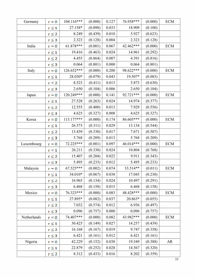
The third column in Appendix Table 2 displays the estimated trace statistic; the fifth column

shows the maximum eigenvalues and followed by its related statistic; the last column lists the

model selected to estimate according to the cointegration test results. Since the trace statistic and

maximum eigenvalues reject the null hypothesis at less than the 5% significance level, it implies

that there exist cointegration relations among variables. In this regard, an ECM will be chosen for

analysis.

The results for the whole sample in Appendix Table 2-1 show that only Côte d'Ivoire and

Nigeria lack a long-run relationship among variables, thus an AR model is used for these two

countries. The remaining 27 countries exhibit a cointegration relation, therefore an ECM is suitable

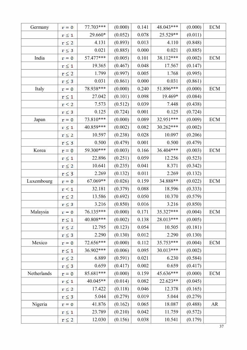
for the statistical analysis. The results for Period I (the duration before December 1986) in

Appendix Table 2-2 indicate that Denmark and Nigeria do not have cointegraion relation and an AR

model is applied. The other 27 countries exhibit cointegration relation and as such the ECM is used.

Likewise, results for Period II (from January 1987 to December 1998) in Appendix Table 2-3

suggest that Austria, Colombia, Côte d’Ivoire, Japan, Nigeria, Portugal, USA, and Venezuela do not

exhibit a cointegration relation, thus the AR model is sufficient for analysis, while the ECM is used

in the remaining 21 countries. In the same way, as displayed in Appendix Table 2-4 for Period III

(the duration after January 1999), variables in Canada, Finland, Japan, Korea, U.K., and Venezuela

are not cointegrated and an AR model is used, whereas the ECM is applied in the remaining 23

countries for the statistical analysis.

11

In sum, the general result of this analysis is that a long-run relationship in our four-variable

model is evident for most of the countries both in the case of full sample and three sub-periods.

4.3. Hansen’s Stability Tests

In this section, we apply Mork (1989) and Mork et al. (1994) and use real oil price increases

and decreases as separation variables from the parameter stability test results. To assess the stability

of parameter estimates, Hansen’s (1992) stability test can be utilized to determine whether the

consumer price indexes respond asymmetrically or symmetrically to oil price movements. An

advantage of this test is that it does not require selecting potential structural break points. Moreover,

no special treatment of lagged dependent variables is required (Hansen, 1992), but the test requires

variables to be stationary. The Hansen stability test produces two types of statistics: a joint test

statistic and an individual test statistic. Individual test statistic represents the stability of each

parameter in the equation, while the joint test assesses the stability of all the parameters jointly in

the entire equation.

Unlike the previous papers, we do not employ positive and negative oil price change as

separation variables arbitrarily in the model. Rather, it is determined by the test results. To test the

asymmetric transmission mechanism from oil prices to inflation in the four-variable model, we opt

for Hansen’s individual test statistics. We do so because oil price increases may or may not have

different impacts on inflation compared with oil price decreases. The results are provided in

Appendix Table 3-1 for the entire sample and in Appendix Tables 3-2 to 3-4 for three sub-periods.

To complete the parameter stability test, we first set the maximum lag periods at 12 and

determine the optimal lag length in equation by minimizing the AIC. Next, the null hypothesis of

stable estimates is rejected if the individual test statistics are significant. The period of a statistically

significant lag variable is used as demarcation point(s) for asymmetry. So we select the significant

estimates of real oil prices as asymmetric variables. To save space, only the estimates of real oil

prices are displayed in Appendix Table 3.

The results in Appendix Table 3-1 for the entire sample report that individual parameters of

12

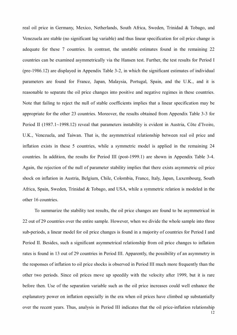
real oil price in Germany, Mexico, Netherlands, South Africa, Sweden, Trinidad & Tobago, and

Venezuela are stable (no significant lag variable) and thus linear specification for oil price change is

adequate for these 7 countries. In contrast, the unstable estimates found in the remaining 22

countries can be examined asymmetrically via the Hansen test. Further, the test results for Period I

(pre-1986.12) are displayed in Appendix Table 3-2, in which the significant estimates of individual

parameters are found for France, Japan, Malaysia, Portugal, Spain, and the U.K., and it is

reasonable to separate the oil price changes into positive and negative regimes in these countries.

Note that failing to reject the null of stable coefficients implies that a linear specification may be

appropriate for the other 23 countries. Moreover, the results obtained from Appendix Table 3-3 for

Period II (1987.1~1998.12) reveal that parameters instability is evident in Austria, Côte d’Ivoire,

U.K., Venezuela, and Taiwan. That is, the asymmetrical relationship between real oil price and

inflation exists in these 5 countries, while a symmetric model is applied in the remaining 24

countries. In addition, the results for Period III (post-1999.1) are shown in Appendix Table 3-4.

Again, the rejection of the null of parameter stability implies that there exists asymmetric oil price

shock on inflation in Austria, Belgium, Chile, Colombia, France, Italy, Japan, Luxembourg, South

Africa, Spain, Sweden, Trinidad & Tobago, and USA, while a symmetric relation is modeled in the

other 16 countries.

To summarize the stability test results, the oil price changes are found to be asymmetrical in

22 out of 29 countries over the entire sample. However, when we divide the whole sample into three

sub-periods, a linear model for oil price changes is found in a majority of countries for Period I and

Period II. Besides, such a significant asymmetrical relationship from oil price changes to inflation

rates is found in 13 out of 29 countries in Period III. Apparently, the possibility of an asymmetry in

the responses of inflation to oil price shocks is observed in Period III much more frequently than the

other two periods. Since oil prices move up speedily with the velocity after 1999, but it is rare

before then. Use of the separation variable such as the oil price increases could well enhance the

explanatory power on inflation especially in the era when oil prices have climbed up substantially

over the recent years. Thus, analysis in Period III indicates that the oil price-inflation relationship

13

can better be explained by taking price asymmetry into consideration.

4.4. Estimated Models

Before estimating equations, some preliminary tests to determine the appropriate form of the

empirical models must be made. Technically, some well-known statistical properties, the integration,

the long-run (cointegration) relationship, and the number of lags, ought to be determined. Equally

important, the stability of oil price parameters in each equation must be tested as well. Finally, the

estimated equations are then specified from the test results previously carried out in the earlier

sections 4.2 and 4.3. From the results in Appendix Table 2 and Appendix Table 3, cointegration and

asymmetrical relationship between oil prices and inflation are determined. As stated in section 3,

therefore, four main models are specified as shown in equation (1) through equation (4).

The results of the estimated models are reported in Appendix Table 4, only coefficients of real

oil price changes are shown for analysis. The current and lagged coefficients are displayed in

columns 4 to 11. Coefficients with positive (+) or negative (-) sign represent an asymmetrical

relationship between oil prices and inflation rates, or a linear relationship otherwise. In addition, the

last three columns in Appendix Table 4 show total symmetrical or asymmetrical impact of oil price

changes on inflation rates. Note that in Appendix Table 4, all the current and delayed coefficients

(both significant and insignificant parameters) of the real oil price changes are reported in order to

illustrate the contemporaneous and cumulative impact of oil prices on inflation. For the other

variables, coefficients with t-statistics less than one are discarded gradually in estimation

procedures according to the parsimonious principle.

From the estimated results in Appendix Table 4, it is evident that the current responses of

inflation rates to oil price changes are larger than the responses during the lagged periods for about

one half of the countries. For instance, the current impacts of oil price change on inflation rates are

greater than that in delayed periods for 15 out of 29 countries over the entire sample (13 out of 15

countries exhibit the asymmetrical relationship); the current responses of inflation to oil price

changes are larger than the responses during the lagged periods for 13 countries in Period I (five out

14

of 13 countries exhibit the asymmetrical relationship); the inflation rates in response to the current

oil price changes are larger than that to lagged oil price changes for 13 countries in Period II (four

out of 13 countries exhibit the asymmetrical relationship); and the oil price transmissions are higher

in current period than that in delayed period for 17 countries in Period III (ten out of 17 countries

exhibit the asymmetrical relationship).

As is to be expected, two important consequences of our estimated results are obtained. First,

as summarized in Table 2, the relationship between oil price changes and inflation rates in 20 out of

27 countries is asymmetrical over the entire sample period, while a majority of them is linear in

each sub-period. A possible explanation for this fact may be attributed to structural breaks detected

in oil price time series. That is to say, after dividing the time series properly according to important

events in the world oil market, a linear model seems to be more acceptable in each sub-period.

Without a doubt, this result not only helps justify the partition of our data set into three independent

periods but also makes sense for our analysis.

Second, as shown in Table 3, responses of inflation in Period I are greater than that in Period

II more than half of the countries. Additionally, it is observed that coefficients in Period I are larger

than that in Period III for half of the countries. In other words, the magnitude of oil price

transmission is greater in the 1970s-1980s than that in the recent twenty years. Well known in

political arena, the global economy has experienced two oil crises (the 1973/74 Arab oil embargo

and the 1978/79 Iranian revolution) and their dramatic influence of oil price changes on inflation

was unprecedented. The result is in agreement with that by Blanchard and Galí (2007) and De

Gregorio et al. (2007): a decline in degrees of transmission from oil price shocks to inflation was

particularly evident in the 2000s.

4.5. Causality Tests

An important issue in estimating model is to determine whether movements in one variable

15

are caused by movements in another. We apply the Granger (1969) model2 to test short-run

reactions from oil price changes to inflation rates based on the four-variable model as specified in

equation (1) and (2), in the absent of a cointegration relation. Failing to reject the null hypothesis

0: 210 pH 3 for the symmetrical model or failing to reject the null hypothesis

0: 22110 ppH for asymmetrical model implies that oil price changes do

not Granger-cause inflation. On the other hand, if cointegration relationship exists in the model, an

error correction term is required in testing Granger causality as shown in equation (3) and (4),

where denotes the speed of adjustment . Failing to reject the null hypothesis

0: 210 pH and 0 for symmetrical model or failing to reject the null

hypothesis 0: 22110 ppH and 0 for asymmetrical model implies that

oil price changes do not Granger-cause inflation. Table 4 shows the results of these Granger

causality tests.

According to the results from Table 4, we find evidence of Granger causality from oil price

shocks to inflation rates in almost all countries. Needless to say, a significant causality is found in

27 out of 29 countries (except Côte d’Ivoire and Nigeria) over the entire period. In a similar vein,

oil price changes Granger-cause inflation in 28 countries (except Denmark) for the period before

1986; evidence of oil price changes causes inflation is obtained in 21 countries (except Austria,

Colombia, Côte d’Ivoire, Germany, Japan, Nigeria, Portugal, and Venezuela) for the period during

1987 and 1998; and a significant causality from oil price shocks to inflation is observed in 27

countries (except Norway and Venezuela) for the period after 1999.

Based on the Granger’s test results, the causality from oil price changes to inflation rates is

more significant when a cointegration relationship is included. Moreover, our results show that oil

price changes cause inflation rates even when a linear relationship is considered. It is apparent that

2 The basic idea of Granger causality theory is to test the null hypothesis that changes in one variable are not able to predict the other. 3 The feasibility of the Granger causality tests depends on the stationarity features of the system. If the series are stationary, the null hypothesis of no Granger causality can be tested by standard Wald tests (Lütkepohl, 1991).

16

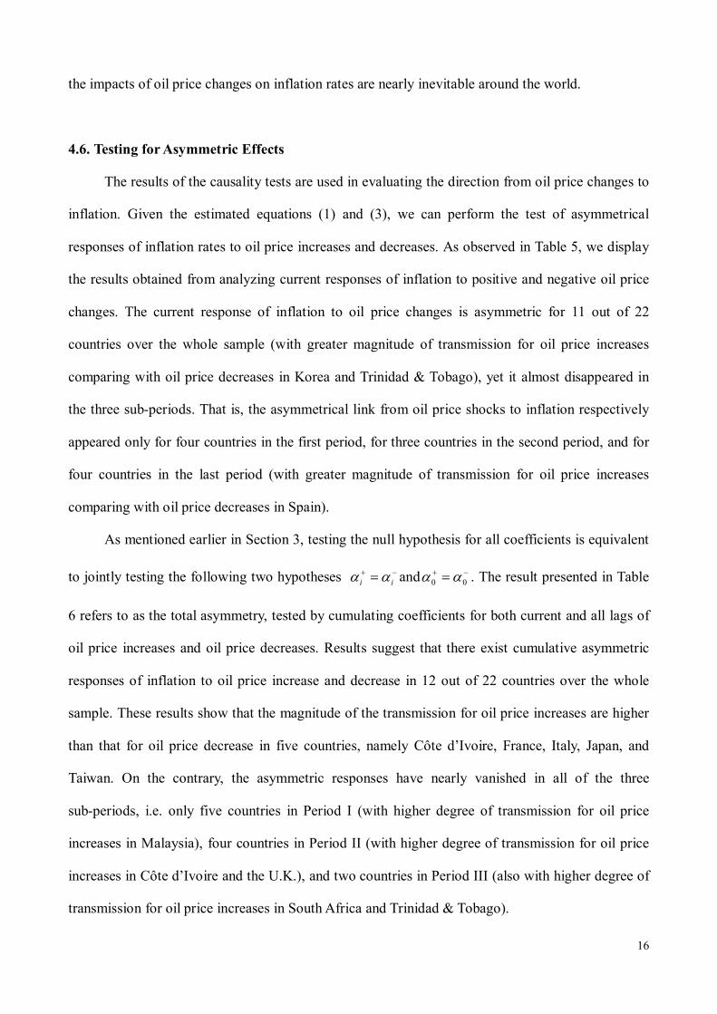
the impacts of oil price changes on inflation rates are nearly inevitable around the world.

4.6. Testing for Asymmetric Effects

The results of the causality tests are used in evaluating the direction from oil price changes to

inflation. Given the estimated equations (1) and (3), we can perform the test of asymmetrical

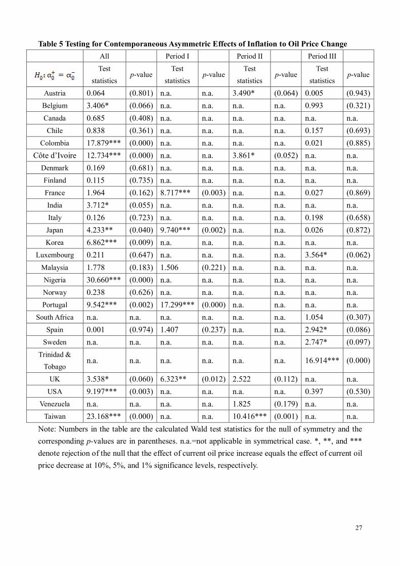
responses of inflation rates to oil price increases and decreases. As observed in Table 5, we display

the results obtained from analyzing current responses of inflation to positive and negative oil price

changes. The current response of inflation to oil price changes is asymmetric for 11 out of 22

countries over the whole sample (with greater magnitude of transmission for oil price increases

comparing with oil price decreases in Korea and Trinidad & Tobago), yet it almost disappeared in

the three sub-periods. That is, the asymmetrical link from oil price shocks to inflation respectively

appeared only for four countries in the first period, for three countries in the second period, and for

four countries in the last period (with greater magnitude of transmission for oil price increases

comparing with oil price decreases in Spain).

As mentioned earlier in Section 3, testing the null hypothesis for all coefficients is equivalent

to jointly testing the following two hypotheses ii and 00 . The result presented in Table

6 refers to as the total asymmetry, tested by cumulating coefficients for both current and all lags of

oil price increases and oil price decreases. Results suggest that there exist cumulative asymmetric

responses of inflation to oil price increase and decrease in 12 out of 22 countries over the whole

sample. These results show that the magnitude of the transmission for oil price increases are higher

than that for oil price decrease in five countries, namely Côte d’Ivoire, France, Italy, Japan, and

Taiwan. On the contrary, the asymmetric responses have nearly vanished in all of the three

sub-periods, i.e. only five countries in Period I (with higher degree of transmission for oil price

increases in Malaysia), four countries in Period II (with higher degree of transmission for oil price

increases in Côte d’Ivoire and the U.K.), and two countries in Period III (also with higher degree of

transmission for oil price increases in South Africa and Trinidad & Tobago).

17

5. Conclusion

A vast volume of past research has examined the macroeonomic response to oil price shocks

with a particular emphasis on real economic activity. Relatively few analyses have tackled the

related question of the effect of oil prices on inflation rates. The purpose of this paper is to examine

the relationship between real oil price changes and the inflation in the framework of Mork’s (1989)

asymmetrical model. To provide better insight into the transmission mechanism, we divide the data

into three periods on the basis of major historical events in the world oil market. This analysis has

supported several conclusions as follows:

First of all, evidence from the analysis supports the existence long-run asymmetric responses

of inflation (entire sample) to real oil price increases and decreases for a majority of countries.

However, the impacts of real oil price changes on inflation are nearly linear in all the three

sub-periods. A possible explanation for this outcome may emanate from a lack of structural breaks

taken place in sub-periods. In other words, after dividing the time series according to important

events, a linear model is much more acceptable for each sub-period. Needless to say, this outcome

further gives us a convincing argument for the division of our sample period.

Second, results of the oil price transmission mainly suggest that current responses of inflation

to real oil price changes are larger than that in the lagged periods. Generally, the cumulative impact

of real oil price increase is greater than the cumulative impact of real oil price decrease.

Third, results from the Granger causality indicate that the direction from real oil price

changes to the inflation is almost completely predictable in both asymmetrical and linear case. In

addition, test results of the Granger causality are most statistically significant when a cointegration

relationship is included in the model.

Finally, by separating the data into three periods based on the important events, the oil price

transmission is typically higher in Period I than that in both Period II and III: a result in line with

the empirical observations that the oil price transmission is more profound in the 1970s-1980s than

in the 1990s and 2000s. As is well known, the global economy experienced two major oil crises in

the 1970s and 1980s that ushered in significant inflation. Furthermore, the recent oil price hike is

18

mainly the result of robust world economy and thus the degree of oil price transmission into

inflation is relatively low and very stable in the last decade. Our finding is also consistent with the

result of Blanchard and Galí (2007) and De Gregorio et al. (2007) that a decline in pass-through

from oil price shocks to inflation has became more evident in the last ten years.

19

References

Bernanke, B.S., M. Gertler, and M. Watson (1997), “Systematic Monetary Policy and the Effects of

Oil Price Shocks,” Brookings Papers on Economic Activity, (1), 91-157.

Blanchard, O. and J. Galí (2007), “The Macroeconomic Effects of Oil Price Shocks: Why Are the

2000s So Different From the 1970s?” NBER Working Paper, No.13368.

Burbidge, J. and A. Harrison (1984), “Testing for the Effects of Oil-Price Rises Using Vector

Autoregressions,” International Economic Review, 25, 459-484.

Cologini, A. and M. Manera (2008), “Oil Prices, Inflation and Interest Rates in A Structural

Cointegrated VAR Model for the G-7 Countries,” Energy Economics, 38, 856-888.

Cuñado, J. and F. Pérez de Gracia (2003), “Do Oil Price Shocks Matter? Evidence from Some

European Countries,” Energy Economics, 25, 137-154.

Cuñado, J. and F. Pérez de Gracia (2005), “Oil Prices, Economic Activity and Inflation: Evidence

for Some Asian Countries,” The Quarterly Review of Economics and Finance, 45, 65-83.

De Gregorio, J., O. Landerretche, and C. Neilson (2007), “Another Pass-Through Bites The Dust?

Oil Prices and Inflation,” Economia, 7(2), 155-196.

Frey, G. and M. Manera (2007), “Econometric Models of Asymmetric Price Transmission,” Journal

of Economic Surveys, 21(2), 349-415.

Gisser, M. and T.H. Goodwin (1986), “Crude Oil and the Macroeconomy: Tests of Some Popular

Notions,” Journal of Money, Credit, and Banking, 18, 95-103.

Granger, C.W.J. (1969), “Investigating Causal Relations by Econometric Models and

Cross-Spectral Methods,” Econometrica, 37, 424-439.

Hamilton, J.D. (1983), “Oil and the Macroeconomy since World War II,” Journal of Political

Economy, 91, 228-248.

Hamilton, J.D. (1996), “This Is What Happened to the Oil Price-Macroeconomy Relationship,”

Journal of Monetary Economics, 38, 215-220.

Hamilton, J.D. (2003), “What Is An Oil Shock?” Journal of Econometrics, 113, 363-398.

Hansen, B.E. (1992), “Testing for Parameter Instability in Linear Models,” Journal of Policy

20

Modeling, 14(4), 517-533.

Hooker, M.A. (1999), “Oil and the Macroeconomy Revisited,” Federal Reserve Board (FEDS)

Working Paper, 43.

Huang, B.N., M.J. Huang, and H.P. Peng (2005), ”The Asymmetry of the Impact of Oil Price

Shocks on Economic Activities: An Application of the Multivariate Threshold Model,” Energy

Economics, 27, 455-476.

Huang, B.N. (2008), “Factors Affecting an Economy’s Tolerance and Delay of Response to the

Impact of a Positive Oil Price Shock,” The Energy Journal, 29(4), 1-34.

Huntington, H.G. (2005), “The Economic Consequences of Higher Crude Oil Prices,” Final Report,

Energy Modeling Forum Special Report, 9, Stanford University.

Johansen, S. (1988), “Statistical and Hypothesis Testing of Cointegration Vectors,” Journal of

Economic Dynamics and Control, 12, 231-254.

Kilian, L. (2008), “Exogenous Oil Supply Shocks: How Big Are They and How Much Do They

Matter for the U.S. Economy?” The Review of Economics and Statistics, 90(2), 216-240.

Krichene, N. (2006), “World Crude Oil Markets: Monetary Policy and the Recent Oil Shock,” IMF

Working Paper, No. 0662.

Krugman, P. (1983), “Oil Shocks and Exchange Rate Dynamics,” in J.A. Frankel (ed.), Exchange

Rates and International Macroeconomics, Chicago: University of Chicago Press.

Lee, K., S. Ni, and R.A. Ratti (1995), “Oil Shocks and the Macroeconomy: The Role of Price

Variability,” The Energy Journal, 16, 39-56.

Lütkepohl, H. (1991), Introduction to Multiple Time Series Analysis, Springer-Verlag, Berlin.

Mork, K.A. (1989), “Oil and Macroeconomy When Prices Go Up and Down: An Extension of

Hamilton’s Results,” Journal of Political Economy, 97(3), 740–744.

Mork, K.A., Ø. Olsen, and H.T. Mysen (1994), “Macroeconomic Responses to Oil Price Increases

and Decreases in Seven OECD Countries,” The Energy Journal, 15(4), 19-35.

Phillips, P.C.B. and P. Perron (1988), “Testing for A Unit Root in Time Series Regression,”

Biometrika, 75(2), 335-346.

21

Rogoff, K.S. (1991), “Oil, Productivity, Government Spending and the Real Yen-Dollar Exchange

Rate,” Pacific Basin Working Paper Series, No.91-06, from Federal Reserve Bank of San

Francisco.

22

Table 1 Sample Countries and Data Periods

Country Data period Number of Observations (T)

Austria 1971:01~2008:02 446

Belgium 1957:01~2008:02 614

Canada 1957:01~2008:03 615

Chile 1977:01~2007:12 372

Colombia 1964:01~2008:04 532

Côte d’Ivoire 1964:01~2008:02 530

Denmark 1967:01~2008:03 495

Finland 1957:01~2008:01 613

France 1957:01~2008:02 614

Germany 1960:01~2008:02 578

India 1957:01~2008:03 615

Italy 1971:01~2008:02 446

Japan 1957:01~2008:03 615

Korea 1970:01~2008:02 458

Luxembourg 1970:01~2008:02 458

Malaysia 1971:01~2008:03 447

Mexico 1960:01~2008:01 577

Netherlands 1964:11~2008:02 520

Nigeria 1964:01~2008:03 531

Norway 1971:08~2008:03 440

Portugal 1966:12~2008:01 494

South Africa 1960:01~2008:03 579

Spain 1974:01~2008:02 410

Sweden 1957:01~2008:03 615

Trinidad & Tobago 1964:12~2008:03 520

United Kingdom 1964:01~2008:03 531

USA 1957:01~2008:04 616

Venezuela 1964:01~2008:01 529

Taiwan 1970:12~2008:03 448

23

Table 2 Total Effects of Inflation Rates to Symmetric and Asymmetric Oil Price Shocks

Symmetrical Impacted Countries

Ratio of

Symmetrical

relative to Total

Asymmetry Impacted Countries

Ratio of

Asymmetrical

relative to Total

Total Impacted

Countries

Full

Sample

Germany, Mexico, Netherlands, South

Africa, Sweden, Trinidad & Tobago,

Venezuela

7/27

Austria, Belgium, Canada, Colombia,

Côte d’Ivoire, Denmark, Finland,

France, India, Italy, Japan, Korea,

Luxembourg, Malaysia, Nigeria,

Norway, Portugal, UK, USA, Taiwan

20/27 27

Period I

Belgium, Canada, Chile, Côte d’Ivoire,

Finland, Germany, India, Italy, Korea,

Luxembourg, Malaysia, Netherlands,

Nigeria, South Africa, Sweden, Trinidad

& Tobago, USA, Venezuela, Taiwan

19/24 France, Japan, Portugal, Spain, UK 5/24 24

Period II

Belgium, Chile, Denmark, France,

India, Italy, Luxembourg, Malaysia,

Mexico, Nigeria, Norway, South Africa,

Sweden, USA

14/19 Austria, Côte d’Ivoire, UK,

Venezuela, Taiwan 5/19 19

Period III

Canada, Denmark, Finland, Germany,

India, Korea, Mexico, Netherlands

Nigeria, Norway, Portugal, UK, Taiwan

13/24

Austria, Belgium, Chile, France, Italy,

Luxembourg, South Africa, Spain,

Sweden, Trinidad &Tobago, USA

11/24 24

Note: Cumulative responses of inflation to oil price changes are taken into consideration.

24

Table 3 Comparing the Magnitudes of Inflation Responses to Oil Shocks across Three Periods

Period I Period II Period III

Austria S L M

Belgium S M L

Canada S M L

Chile S M L

Colombia L S M

Côte d’Ivoire L M S

Denmark S M L

Finland S M L

France M S L

Germany S M L

India M S L

Italy L S M

Japan L S M

Korea L S M

Luxembourg L M S

Malaysia L M S

Mexico S M L

Netherlands L M S

Nigeria S L M

Norway S M L

Portugal L S M

South Africa S M L

Spain L S M

Sweden S L M

Trinidad & Tobago M S L

UK L S M

USA M S L

Venezuela L M S

Taiwan L M S

Summary Period I>II: 17/29 Period II>III: 9/29 Period I>III: 13/29

Note: L, M, and S represent respectively the largest, the medium, and the smallest response of

inflation rates to oil price shocks. In comparison with period I, II, and III, the measures in the table

are taken based on the size of cumulative effects.

25

Table 4 Granger Causality Tests from Oil Price Changes to Inflation Rates

Null hypothesis: All Period I Period II Period III

lroilp lcpi M Asy. Statistics p-value M Asy. Statistics p-value M Asy. Statistics p-value M Asy. Statistics p-value

Austria E Y 12.504*** (0.000) E N 31.361*** (0.000) A Y 1.305 (0.275) E Y 4.902*** (0.003)

Belgium E Y 4.114*** (0.001) E N 10.117*** (0.000) E N 17.404*** (0.000) E Y 2.964** (0.036)

Canada E Y 37.395*** (0.000) E N 21.396*** (0.000) E N 35.514*** (0.000) A Y 9.344*** (0.000)

Chile E Y 29.969*** (0.000) E N 7.366*** (0.001) E N 19.433*** (0.000) E Y 7.116*** (0.000)

Colombia E Y 6.302*** (0.000) E N 32.138*** (0.000) A N 0.672 (0.414) E Y 5.288*** (0.002)

Côte d’Ivoire A Y 2.142 (0.119) E N 17.928*** (0.000) A Y 1.328 (0.263) E N 8.206*** (0.001)

Denmark E Y 15.526*** (0.000) A N 0.000 (0.989) E N 8.594*** (0.000) E N 7.314*** (0.001)

Finland E Y 4.419*** (0.001) E N 24.062*** (0.000) E N 22.917*** (0.000) A N 5.703** (0.019)

France E Y 6.224*** (0.000) E Y 22.984*** (0.000) E N 28.761*** (0.000) E Y 5.363*** (0.000)

Germany E N 13.600*** (0.000) E N 29.036*** (0.000) E N 0.244 (0.784) E N 9.973*** (0.000)

India E Y 12.507*** (0.000) E N 9.256*** (0.000) E N 5.982*** (0.003) E N 9.090*** (0.000)

Italy E Y 23.663*** (0.000) E N 43.143*** (0.000) E N 28.822*** (0.000) E Y 9.571*** (0.000)

Japan E Y 5.006*** (0.002) E Y 14.188*** (0.000) A N 0.194 (0.941) A Y 2.398* (0.096)

Korea E Y 22.281*** (0.000) E N 13.441*** (0.000) E N 19.647*** (0.000) A N 4.103** (0.045)

Luxembourg E Y 8.170*** (0.000) E N 16.261*** (0.000) E N 38.837*** (0.000) E Y 4.594*** (0.001)

Malaysia E Y 6.741*** (0.000) E Y 12.784*** (0.000) E N 14.235*** (0.000) E N 6.574*** (0.002)

Mexico E N 24.901*** (0.000) E N 2.435** (0.015) E N 11.051*** (0.000) E N 10.173*** (0.000)

Netherlands E N 19.803*** (0.000) E N 23.121*** (0.000) E N 2.617** (0.038) E N 2.606** (0.041)

Nigeria A Y 0.125 (0.883) A N 4.882** (0.028) A N 0.315 (0.576) E N 2.132 (0.125)

Norway E Y 6.968*** (0.000) E N 59.607*** (0.000) E N 10.252*** (0.000) E N 2.520* (0.086)

Portugal E Y 44.242*** (0.000) E Y 21.596*** (0.000) A N 0.381 (0.538) E N 28.015*** (0.000)

South Africa E N 51.609*** (0.000) E N 50.746*** (0.000) E N 20.108*** (0.000) E Y 12.632*** (0.000)

26

Spain E Y 5.212*** (0.000) E Y 35.110*** (0.000) E N 10.242*** (0.000) E Y 6.664*** (0.000)

Sweden E N 14.982*** (0.000) E N 81.232*** (0.000) E N 22.879*** (0.000) E Y 2.484* (0.065)

Trinidad & Tobago E N 3.547** (0.015) E N 6.946*** (0.000) E N 31.960*** (0.000) E Y 3.966** (0.010)

UK E Y 5.293*** (0.000) E N 16.560*** (0.000) E N 12.122*** (0.000) A N 10.181*** (0.002)

USA E Y 5.910*** (0.000) E N 15.677*** (0.000) A Y 11.788*** (0.000) E Y 3.809** (0.012)

Venezuela E N 13.551*** (0.000) E N 36.956*** (0.000) A Y 0.449 (0.639) A N 0.875 (0.352)

Taiwan E Y 6.238*** (0.000) E N 8.179*** (0.000) E Y 5.155*** (0.002) E N 9.824*** (0.000)

Note: The null hypothesis that lag values of real oil price changes do not Granger-cause inflation is tested. Numbers in the table are 2 -statistics and

the corresponding p-values are in the parentheses. *, **, and *** indicate statistically significant at 10%, 5%, and 1% level, respectively. M=A

denotes AR model while M=E denotes ECM. Asy.=Y stands for asymmetrical impact of oil price changes on inflation rates while Asy.=N stands for

symmetrical impact of oil price changes on inflation rates.

27

Table 5 Testing for Contemporaneous Asymmetric Effects of Inflation to Oil Price Change

All Period I Period II Period III

Test

statistics p-value

Test

statistics p-value

Test

statistics p-value

Test

statistics p-value

Austria 0.064 (0.801) n.a. n.a. 3.490* (0.064) 0.005 (0.943)

Belgium 3.406* (0.066) n.a. n.a. n.a. n.a. 0.993 (0.321)

Canada 0.685 (0.408) n.a. n.a. n.a. n.a. n.a. n.a.

Chile 0.838 (0.361) n.a. n.a. n.a. n.a. 0.157 (0.693)

Colombia 17.879*** (0.000) n.a. n.a. n.a. n.a. 0.021 (0.885)

Côte d’Ivoire 12.734*** (0.000) n.a. n.a. 3.861* (0.052) n.a. n.a.

Denmark 0.169 (0.681) n.a. n.a. n.a. n.a. n.a. n.a.

Finland 0.115 (0.735) n.a. n.a. n.a. n.a. n.a. n.a.

France 1.964 (0.162) 8.717*** (0.003) n.a. n.a. 0.027 (0.869)

India 3.712* (0.055) n.a. n.a. n.a. n.a. n.a. n.a.

Italy 0.126 (0.723) n.a. n.a. n.a. n.a. 0.198 (0.658)

Japan 4.233** (0.040) 9.740*** (0.002) n.a. n.a. 0.026 (0.872)

Korea 6.862*** (0.009) n.a. n.a. n.a. n.a. n.a. n.a.

Luxembourg 0.211 (0.647) n.a. n.a. n.a. n.a. 3.564* (0.062)

Malaysia 1.778 (0.183) 1.506 (0.221) n.a. n.a. n.a. n.a.

Nigeria 30.660*** (0.000) n.a. n.a. n.a. n.a. n.a. n.a.

Norway 0.238 (0.626) n.a. n.a. n.a. n.a. n.a. n.a.

Portugal 9.542*** (0.002) 17.299*** (0.000) n.a. n.a. n.a. n.a.

South Africa n.a. n.a. n.a. n.a. n.a. n.a. 1.054 (0.307)

Spain 0.001 (0.974) 1.407 (0.237) n.a. n.a. 2.942* (0.086)

Sweden n.a. n.a. n.a. n.a. n.a. n.a. 2.747* (0.097)

Trinidad &

Tobago n.a. n.a. n.a. n.a. n.a. n.a. 16.914*** (0.000)

UK 3.538* (0.060) 6.323** (0.012) 2.522 (0.112) n.a. n.a.

USA 9.197*** (0.003) n.a. n.a. n.a. n.a. 0.397 (0.530)

Venezuela n.a. n.a. n.a. n.a. 1.825 (0.179) n.a. n.a.

Taiwan 23.168*** (0.000) n.a. n.a. 10.416*** (0.001) n.a. n.a.

Note: Numbers in the table are the calculated Wald test statistics for the null of symmetry and the

corresponding p-values are in parentheses. n.a.=not applicable in symmetrical case. *, **, and ***

denote rejection of the null that the effect of current oil price increase equals the effect of current oil

price decrease at 10%, 5%, and 1% significance levels, respectively.

28

Table 6 Testing for Total Asymmetric Effects of Inflation to Oil Price Change

All Period I Period II Period III

p

ii

p

iiH

000 : i

Test

statistics p-value i

Test

statistics p-value i

Test

statistics p-value i

Test

statistics p-value

Austria 0,5 1.323 (0.251) n.a. n.a. 0,2 10.030*** (0.002) 0,6 0.473 (0.493)

Belgium 0,2 0.507 (0.477) n.a. n.a. n.a. n.a. 0,1 1.538 (0.218)

Canada 0,4 3.308* (0.070) n.a. n.a. n.a. n.a. n.a. n.a.

Chile 0,2 1.639 (0.201) n.a. n.a. n.a. n.a. 0,1 0.011 (0.916)

Colombia 0,1 23.828*** (0.000) n.a. n.a. n.a. n.a. 0,1 2.026 (0.158)

Côte d’Ivoire 0,2 29.616*** (0.000) n.a. n.a. 0,6,10 10.619*** (0.001) n.a. n.a.

Denmark 0,3,5 4.535** (0.034) n.a. n.a. n.a. n.a. n.a. n.a.

Finland 0,6,12 1.459 (0.228) n.a. n.a. n.a. n.a. n.a. n.a.

France 0,2,3,12 7.843*** (0.005) 0,3 9.584*** (0.002) n.a. n.a. 0,1,4,6 1.512 (0.222)

India 0,4,6 13.800*** (0.000) n.a. n.a. n.a. n.a. n.a. n.a.

Italy 0,1,2 3.488* (0.063) n.a. n.a. n.a. n.a. 0,5 0.299 (0.586)

Japan 0,3 5.939** (0.015) 0,3 11.104*** (0.001) n.a. n.a. 0,1 0.557 (0.457)

Korea 0,2 10.066*** (0.002) n.a. n.a. n.a. n.a. n.a. n.a.

Luxembourg 0,3,7 0.383 (0.536) n.a. n.a. n.a. n.a. 0,5,12 1.131 (0.290)

Malaysia 0,1,5 2.614 (0.107) 0,1 5.665** (0.018) n.a. n.a. n.a. n.a.

Nigeria 0,1 28.412*** (0.000) n.a. n.a. n.a. n.a. n.a. n.a.

Norway 0,4,12 1.519 (0.219) n.a. n.a. n.a. n.a. n.a. n.a.

Portugal 0,1 14.747*** (0.000) 0,1 11.547*** (0.001) n.a. n.a. n.a. n.a.

South Africa n.a. n.a. n.a. n.a. n.a. n.a. 0,1 5.629** (0.020)

Spain 0,1,7 0.270 (0.604) 0,1 0.173 (0.678) n.a. n.a. 0,1 1.450 (0.231)

Sweden n.a. n.a. n.a. n.a. n.a. n.a. 0,1 0.019 (0.892)

29

Trinidad & Tobago n.a. n.a. n.a. n.a. n.a. n.a. 0,4 17.848*** (0.000)

UK 0,5,7,12 0.831 (0.362) 0,2 5.881** (0.016) 0,3 3.305* (0.071) n.a. n.a.

USA 0,4,9 0.031 (0.859) n.a. n.a. n.a. n.a. 0,1 1.155 (0.285)

Venezuela n.a. n.a. n.a. n.a. 0,1 0.538 (0.464) n.a. n.a.

Taiwan 0,3 15.619*** (0.000) n.a. n.a. 0,2 4.229** (0.042) n.a. n.a.

Note: The null hypothesis is

p

ii

p

ii

00

. Subscript “i” indicates the lag length of asymmetric oil price change, which is determined by Hansen

stability test in estimated equation. Entries are the calculated F statistics for the null of symmetry and the corresponding p-values are in brackets.

n.a.=not applicable in symmetrical case. *, **, and *** denote rejection of the null that the effect of cumulative oil price increase equals the effect of

cumulative oil price decrease at 10%, 5%, and 1% significance levels, respectively.

30

$0

$20

$40

$60

$80

$100

$120

1957 1960 1963 1966 1969 1972 1975 1978 1981 1984 1987 1990 1993 1996 1999 2002 2005 2008

Real (2000 US dollars)Nominal

Figure 1 Oil Prices (U.S. Dollars per Barrel), 1957M1-2008M4.

31

Appendix Table 1 Results of Phillips-Perron Unit Root Tests

Variables ER LCPI LROILP R

Level Difference Level Difference Level Difference Level Difference

Austria -0.679 -7.274*** 8.168 -9.541*** 2.216 -9.868*** -0.221 -8.420***

Belgium -0.781 -8.332*** 8.044 -8.104*** -0.840 -7.154*** -0.954 -8.646***

Canada 2.328 -16.077*** 9.018 -7.710*** 0.014 -16.848*** -0.525 -12.569***

Chile -0.045 -7.020*** 6.204 -4.910*** 1.957 -9.854*** -1.556 -14.675***

Colombia 0.865 -14.864*** 3.011 -6.395*** -1.432 -18.506*** -0.617 -18.662***

Côte d’Ivoire -0.679 -7.227*** 5.628 -7.299*** 2.031 -9.868*** -1.366 -10.635***

Denmark -0.711 -16.445*** 6.444 -16.290*** 0.642 -18.282*** -0.847 -20.329***

Finland -0.672 -7.242*** 4.270 -7.699*** 2.218 -9.867*** 0.176 -10.392***

France -0.284 -19.000*** 6.268 -7.813*** 0.408 -20.385*** -0.711 -22.352***

Germany -1.780 -18.113*** 10.308 -19.173*** 0.876 -19.785*** -1.490 -33.575***

India -0.388 -6.719*** 5.544 -6.734 *** 2.036 -9.842*** -1.239 -62.088***

Italy -0.681 -7.276*** 14.893 -3.746*** 2.107 -9.893*** 0.050 -6.955***

Japan -2.225 -18.304*** 4.538 -23.190*** 0.912 -20.682*** -1.501 -23.522***

Korea -1.169 -8.446*** 12.098 -7.082*** 2.148 -9.979*** 0.111 -11.141***

Luxembourg -0.681 -7.285*** 16.315 -14.221*** 2.178 -10.135*** -0.152 -7.539***

Malaysia 5.137 -6.619*** 7.033 -9.665*** 2.301 -9.835*** -1.503 -8.720***

Mexico 0.490 -9.118*** 7.615 -4.279*** 1.803 -9.975*** -2.236 -5.737***

Netherlands -1.597 -17.055*** 4.345 -20.297*** 0.739 -18.502*** -0.582 -16.626***

Nigeria 0.521 -10.326*** 4.150 -7.476*** 1.546 -10.548*** -0.609 -9.450***

Norway -1.174 -8.030*** 3.663 -7.739*** 2.340 -9.866*** -1.444 -5.719***

Portugal 0.355 -15.413*** 6.613 -11.592*** -0.374 -18.485*** -0.476 -22.088***

South Africa 0.130 -7.584*** 6.768 -4.680*** 1.949 -9.984*** -2.603 -4.069***

Spain -0.685 -7.280*** 8.874 -6.365*** 2.110 -9.925*** 0.124 -9.341***

Sweden -0.825 -8.026*** 4.851 -8.041*** 2.350 -9.822*** -0.098 -10.455***

Trinidad & Tobago

0.182 -5.412*** 9.372 -7.416*** 1.880 -9.960*** -0.963 -6.774***

UK -0.060 -16.717*** 8.940 -10.301*** 0.351 -19.118*** -0.824 -15.767***

USA -1.465 -17.556*** 13.122 -7.189*** 0.680 -20.537*** -1.261 -16.009***

Venezuela 1.958 -9.181*** 12.229 -2.121** 0.483 -10.364*** -3.115 -9.245***

Taiwan -0.397 -6.907*** 1.178 -12.709*** 2.462 -9.985*** -1.227 -7.493***

Note: ER represents the exchange rate. R is the interest rate. LCPI and LROILP represent respectively the consumer price index and real oil price after logarithmic transformation. Numbers in the table are t-statistics. *, ** and *** denote rejection for the unit root null at 10%, 5%, and 1% significance levels, respectively.

32

Appendix Table 2-1 Results of Johansen’s Cointegration Tests (Full Sample)

Trace p-value Eigen value

Max-Eigen p-value Model

Austria 182.550*** (0.000) 0.286 148.370*** (0.000) ECM

34.180* (0.064) 0.043 19.243 (0.127)

14.938 (0.230) 0.023 10.445 (0.296)

4.493 (0.344) 0.010 4.493 (0.344)

Belgium 75.224*** (0.000) 0.069 43.466*** (0.000) ECM

31.758 (0.112) 0.029 18.144 (0.172)

13.614 (0.317) 0.016 9.767 (0.356)

3.847 (0.435) 0.006 3.847 (0.435)

Canada 83.888*** (0.000) 0.109 70.213*** (0.000) ECM

13.675 (0.858) 0.017 10.535 (0.693)

3.141 (0.960) 0.005 2.912 (0.952)

0.229 (0.633) 0.000 0.229 (0.633)

Chile 94.892*** (0.000) 0.135 52.874*** (0.000) ECM

42.018*** (0.008) 0.074 28.157*** (0.007)

13.861 (0.299) 0.022 8.082 (0.538)

5.779 (0.209) 0.016 5.779 (0.209)

Colombia 81.581*** (0.000) 0.087 47.996*** (0.000) ECM

33.585** (0.018) 0.036 19.310* (0.088)

14.275* (0.076) 0.026 14.026* (0.055)

0.249 (0.618) 0.000 0.249 (0.618)

Cote D’Ivior 27.107 (0.850) 0.026 13.963 (0.825) AR

13.144 (0.885) 0.016 8.333 (0.882)

4.810 (0.829) 0.009 4.553 (0.797)

0.258 (0.612) 0.000 0.258 (0.612)

Denmark 98.892*** (0.000) 0.141 74.935*** (0.000) ECM

23.957 (0.202) 0.031 15.341 (0.266)

8.616 (0.402) 0.013 6.297 (0.576)

2.320 (0.128) 0.005 2.320 (0.128)

Finland 76.607*** (0.000) 0.089 57.094*** (0.000) ECM

19.513 (0.457) 0.019 11.597 (0.588)

7.916 (0.474) 0.012 7.621 (0.419)

0.295 (0.587) 0.000 0.295 (0.587)

France 98.820*** (0.000) 0.120 78.074*** (0.000) ECM

20.747 (0.374) 0.026 16.288 (0.209)

4.459 (0.863) 0.007 4.209 (0.837)

0.250 (0.617) 0.000 0.250 (0.617)

33

Germany 104.116*** (0.000) 0.127 76.958*** (0.000) ECM

27.158* (0.098) 0.033 18.909 (0.100)

8.249 (0.439) 0.010 5.927 (0.623)

2.323 (0.128) 0.004 2.323 (0.128)

India 61.878*** (0.001) 0.067 42.462*** (0.000) ECM

19.416 (0.463) 0.024 14.961 (0.292)

4.455 (0.864) 0.007 4.391 (0.816)

0.064 (0.801) 0.000 0.064 (0.801)

Italy 126.652*** (0.000) 0.200 98.622*** (0.000) ECM

28.030* (0.079) 0.043 19.507* (0.083)

8.523 (0.411) 0.013 5.873 (0.630)

2.650 (0.104) 0.006 2.650 (0.104)

Japan 120.249*** (0.000) 0.141 92.721*** (0.000) ECM

27.528 (0.263) 0.024 14.974 (0.377)

12.555 (0.400) 0.013 7.929 (0.556)

4.625 (0.327) 0.008 4.625 (0.327)

Korea 113.177*** (0.000) 0.174 86.605*** (0.000) ECM

26.573 (0.311) 0.029 13.134 (0.544)

13.439 (0.330) 0.017 7.671 (0.587)

5.768 (0.209) 0.013 5.768 (0.209)

Luxembourg 72.225*** (0.001) 0.097 46.014*** (0.000) ECM

26.211 (0.330) 0.024 10.804 (0.768)

15.407 (0.204) 0.022 9.911 (0.343)

5.495 (0.233) 0.012 5.495 (0.233)

Malaysia 67.525*** (0.002) 0.074 33.514** (0.011) ECM

34.010* (0.067) 0.038 17.045 (0.230)

16.965 (0.134) 0.024 10.497 (0.291)

6.468 (0.158) 0.015 6.468 (0.158)

Mexico 76.323*** (0.000) 0.083 48.428*** (0.000) ECM

27.895* (0.082) 0.037 20.863* (0.055)

7.032 (0.574) 0.012 6.936 (0.497)

0.096 (0.757) 0.000 0.096 (0.757)

Netherlands 74.407*** (0.000) 0.082 43.982*** (0.000) ECM

30.425 (0.149) 0.027 14.257 (0.439)

16.168 (0.167) 0.019 9.747 (0.358)

6.421 (0.161) 0.012 6.421 (0.161)

Nigeria 42.229 (0.152) 0.038 19.349 (0.388) AR

22.879 (0.252) 0.028 14.567 (0.320)

8.312 (0.433) 0.016 8.202 (0.359)

34

0.110 (0.740) 0.000 0.110 (0.740)

Norway 157.134*** (0.000) 0.254 126.650*** (0.000) ECM

30.483 (0.148) 0.037 16.484 (0.265)

14.000 (0.289) 0.022 9.605 (0.372)

4.394 (0.357) 0.010 4.394 (0.357)

Portugal 100.346*** (0.000) 0.139 73.608*** (0.000) ECM

26.739 (0.108) 0.036 18.249 (0.121)

8.490 (0.415) 0.015 7.425 (0.440)

1.065 (0.302) 0.002 1.065 (0.302)

South Africa 105.729*** (0.000) 0.140 86.645*** (0.000) ECM

19.084 (0.487) 0.024 13.873 (0.376)

5.211 (0.786) 0.009 5.099 (0.729)

0.112 (0.738) 0.000 0.112 (0.738)

Spain 56.307*** (0.007) 0.091 38.002*** (0.002) ECM

18.305 (0.544) 0.024 9.808 (0.763)

8.497 (0.414) 0.020 8.002 (0.379)

0.496 (0.481) 0.001 0.496 (0.481)

Sweden 101.043*** (0.000) 0.118 76.833*** (0.000) ECM

24.210 (0.192) 0.025 15.507 (0.255)

8.703 (0.394) 0.014 8.340 (0.345)

0.362 (0.547) 0.001 0.362 (0.547)

Trinidad & Tobago 73.665*** (0.000) 0.093 50.395*** (0.000) ECM

23.270 (0.233) 0.025 13.202 (0.434)

10.068 (0.276) 0.018 9.568 (0.242)

0.500 (0.480) 0.001 0.500 (0.480)

UK 77.855*** (0.000) 0.107 59.897*** (0.000) ECM

17.958 (0.569) 0.017 8.941 (0.837)

9.017 (0.364) 0.015 8.199 (0.359)

0.818 (0.366) 0.002 0.818 (0.366)

USA 110.895*** (0.000) 0.135 88.704*** (0.000) ECM

22.191 (0.288) 0.025 15.276 (0.270)

6.915 (0.588) 0.011 6.910 (0.500)

0.005 (0.945) 0.000 0.005 (0.945)

Venezuela 79.392*** (0.000) 0.082 44.691*** (0.000) ECM

34.701** (0.013) 0.043 22.971** (0.027)

11.730 (0.170) 0.022 11.543 (0.129)

0.186 (0.666) 0.000 0.186 (0.666)

Taiwan 55.550*** (0.008) 0.067 30.546** (0.020) ECM

35

25.004 (0.161) 0.032 14.406 (0.333)

10.598 (0.238) 0.019 8.649 (0.317)

1.949 (0.163) 0.004 1.949 (0.163)

Note: Trace=Trace Statistics; Max-Eigen=Maximum Eigenvalue Statistics; AR=Autoregressive Model; ECM=Error Correction Model; r=number of cointegrating relation(s). *, **, and *** indicate statistically significant at 10%, 5%, and 1% levels, respectively.

36

Appendix Table 2-2 Results of Johansen’s Cointegration Tests (Period I: Pre-1986:12)

Trace p-value Eigen value

Max-Eigen p-value Model

Austria 103.351*** (0.000) 0.310 69.515*** (0.000) ECM

33.835* (0.070) 0.101 19.854 (0.106)

13.981 (0.291) 0.047 8.971 (0.437)

5.010 (0.282) 0.026 5.010 (0.282)

Belgium 80.387*** (0.000) 0.089 33.180** (0.012) ECM

47.206*** (0.002) 0.071 25.963** (0.015)

21.243 (0.037) 0.039 14.025* (0.096)

7.218 (0.115) 0.020 7.218 (0.115)

Canada 66.838*** (0.000) 0.105 39.267*** (0.001) ECM

27.571* (0.088) 0.054 19.891* (0.074)

7.679 (0.500) 0.021 7.648 (0.416)

0.031 (0.860) 0.000 0.031 (0.860)

Chile 50.044** (0.031) 0.224 28.700** (0.036) ECM

21.344 (0.337) 0.113 13.510 (0.407)

7.834 (0.483) 0.067 7.812 (0.398)

0.021 (0.884) 0.000 0.021 (0.884)

Colombia 61.753*** (0.002) 0.134 39.341*** (0.001) ECM

22.412 (0.276) 0.058 16.232 (0.212)

6.180 (0.674) 0.022 6.109 (0.599)

0.071 (0.790) 0.000 0.071 (0.790)

Côte d’Ivoire 74.507*** (0.000) 0.138 40.651*** (0.001) ECM

33.856* (0.069) 0.073 20.575* (0.086)

13.281 (0.342) 0.035 9.816 (0.352)

3.466 (0.498) 0.013 3.466 (0.498)

Denmark 44.182 (0.106) 0.082 20.477 (0.309) AR

23.705 (0.213) 0.060 14.787 (0.304)

8.917 (0.373) 0.037 8.874 (0.297)

0.044 (0.834) 0.000 0.044 (0.834)

Finland 71.602*** (0.000) 0.134 51.155*** (0.000) ECM

20.447 (0.393) 0.035 12.795 (0.471)

7.652 (0.503) 0.019 6.971 (0.493)

0.681 (0.409) 0.002 0.681 (0.409)

France 79.272*** (0.000) 0.112 42.146*** (0.000) ECM

37.126*** (0.006) 0.068 25.022** (0.013)

12.104 (0.152) 0.028 10.235 (0.197)

1.869 (0.172) 0.005 1.869 (0.172)

37

Germany 77.703*** (0.000) 0.141 48.043*** (0.000) ECM

29.660* (0.052) 0.078 25.529** (0.011)

4.131 (0.893) 0.013 4.110 (0.848)

0.021 (0.885) 0.000 0.021 (0.885)

India 57.477*** (0.005) 0.101 38.112*** (0.002) ECM

19.365 (0.467) 0.048 17.567 (0.147)

1.799 (0.997) 0.005 1.768 (0.995)

0.031 (0.861) 0.000 0.031 (0.861)

Italy 78.938*** (0.000) 0.240 51.896*** (0.000) ECM

27.042 (0.101) 0.098 19.469* (0.084)

7.573 (0.512) 0.039 7.448 (0.438)

0.125 (0.724) 0.001 0.125 (0.724)

Japan 73.810*** (0.000) 0.089 32.951*** (0.009) ECM

40.859*** (0.002) 0.082 30.262*** (0.002)

10.597 (0.238) 0.028 10.097 (0.206)

0.500 (0.479) 0.001 0.500 (0.479)

Korea 59.300*** (0.003) 0.166 36.404*** (0.003) ECM

22.896 (0.251) 0.059 12.256 (0.523)

10.641 (0.235) 0.041 8.371 (0.342)

2.269 (0.132) 0.011 2.269 (0.132)

Luxembourg 67.069** (0.026) 0.159 34.888** (0.022) ECM

32.181 (0.379) 0.088 18.596 (0.333)

13.586 (0.692) 0.050 10.370 (0.579)

3.216 (0.850) 0.016 3.216 (0.850)

Malaysia 76.135*** (0.000) 0.171 35.327*** (0.004) ECM

40.808*** (0.002) 0.138 28.013*** (0.005)

12.795 (0.123) 0.054 10.505 (0.181)

2.290 (0.130) 0.012 2.290 (0.130)

Mexico 72.656*** (0.000) 0.112 35.753*** (0.004) ECM

36.902*** (0.006) 0.095 30.013*** (0.002)

6.889 (0.591) 0.021 6.230 (0.584)

0.659 (0.417) 0.002 0.659 (0.417)

Netherlands 85.681*** (0.000) 0.159 45.636*** (0.000) ECM

40.045** (0.014) 0.082 22.623** (0.045)

17.422 (0.118) 0.046 12.378 (0.165)

5.044 (0.279) 0.019 5.044 (0.279)

Nigeria 41.876 (0.162) 0.065 18.087 (0.488) AR

23.789 (0.210) 0.042 11.759 (0.572)

12.030 (0.156) 0.038 10.541 (0.179)

38

1.488 (0.223) 0.005 1.488 (0.223)

Norway 113.477*** (0.000) 0.308 66.888*** (0.000) ECM

46.590*** (0.002) 0.149 29.442*** (0.004)

17.148 (0.127) 0.060 11.263 (0.233)

5.884 (0.200) 0.032 5.884 (0.200)

Portugal 99.133*** (0.000) 0.235 63.718*** (0.000) ECM

35.415** (0.047) 0.081 20.135* (0.098)

15.281 (0.211) 0.049 11.976 (0.187)

3.305 (0.525) 0.014 3.305 (0.525)

South Africa 129.399*** (0.000) 0.177 61.492*** (0.000) ECM

67.906*** (0.000) 0.135 45.876*** (0.000)

22.030 (0.140) 0.052 16.817 (0.114)

5.213 (0.566) 0.016 5.213 (0.566)

Spain 127.558*** (0.000) 0.444 90.319*** (0.000) ECM

37.239** (0.030) 0.145 24.187** (0.027)

13.052 (0.360) 0.058 9.134 (0.420)

3.918 (0.425) 0.025 3.918 (0.425)

Sweden 75.713*** (0.000) 0.103 38.777*** (0.001) ECM

36.936*** (0.006) 0.066 24.057** (0.019)

12.879 (0.119) 0.032 11.375 (0.136)

1.505 (0.220) 0.004 1.505 (0.220)

Trinidad & Tobago 78.056*** (0.000) 0.149 41.682*** (0.001) ECM

36.374** (0.037) 0.088 23.809** (0.031)

12.565 (0.400) 0.038 10.080 (0.327)

2.485 (0.681) 0.010 2.485 (0.681)

UK 56.568*** (0.006) 0.119 34.666*** (0.005) ECM

21.901 (0.304) 0.053 14.732 (0.308)

7.169 (0.558) 0.024 6.511 (0.549)

0.658 (0.417) 0.002 0.658 (0.417)

USA 85.165*** (0.000) 0.116 42.675*** (0.002) ECM

42.490* (0.055) 0.058 20.641 (0.208)

21.849 (0.146) 0.046 16.318 (0.132)

5.531 (0.522) 0.016 5.531 (0.522)

Venezuela 99.025*** (0.000) 0.161 47.895*** (0.000) ECM

51.130*** (0.006) 0.091 26.051** (0.047)

25.079* (0.063) 0.061 17.071 (0.105)

8.007 (0.251) 0.029 8.007 (0.251)

Taiwan 66.825*** (0.002) 0.151 30.840** (0.025) ECM

39

35.986** (0.041) 0.114 22.799** (0.043)

13.186 (0.349) 0.040 7.762 (0.576)

5.424 (0.240) 0.028 5.424 (0.240)

Note: Trace=Trace Statistics; Max-Eigen=Maximum Eigenvalue Statistics; AR=Autoregressive Model; ECM=Error Correction Model; r=number of cointegrating relation(s). *, **, and *** indicate statistically significant at 10%, 5%, and 1% levels, respectively.

40

Appendix Table 2-3 Results of Johansen’s Cointegration Tests (Period II: 1987:01-1998:12)

Trace p-value Eigen value

Max-Eigen p-value Model

Austria 50.872 (0.376) 0.173 27.304 (0.173) AR

23.568 (0.855) 0.107 16.242 (0.523)

7.325 (0.991) 0.026 3.764 (0.999)

3.561 (0.804) 0.024 3.561 (0.804)

Belgium 100.950*** (0.000) 0.370 66.431*** (0.000) ECM

34.519* (0.059) 0.112 17.125 (0.226)

17.395 (0.119) 0.083 12.477 (0.160)

4.918 (0.293) 0.034 4.918 (0.293)

Canada 83.384*** (0.000) 0.278 46.863*** (0.000) ECM

36.520*** (0.007) 0.144 22.401** (0.033)

14.120* (0.080) 0.068 10.115 (0.205)

4.005** (0.045) 0.027 4.005 (0.045)

Chile 52.827** (0.016) 0.195 31.216** (0.016) ECM

21.611 (0.321) 0.079 11.862 (0.561)

9.749 (0.301) 0.050 7.455 (0.437)

2.295 (0.130) 0.016 2.295 (0.130)

Colombia 32.593 (0.579) 0.129 19.970 (0.343) AR

12.623 (0.908) 0.049 7.212 (0.945)

5.411 (0.764) 0.037 5.381 (0.693)

0.030 (0.863) 0.000 0.030 (0.863)

Côte d’Ivoire 42.087 (0.156) 0.116 17.812 (0.511) AR

24.274 (0.189) 0.091 13.691 (0.391)

10.583 (0.239) 0.070 10.481 (0.182)

0.102 (0.750) 0.001 0.102 (0.750)

Denmark 54.465** (0.011) 0.203 32.689** (0.010) ECM

21.777 (0.311) 0.091 13.777 (0.384)

8.000 (0.466) 0.054 7.971 (0.382)

0.029 (0.865) 0.000 0.029 (0.865)

Finland 77.069*** (0.003) 0.205 33.108** (0.038) ECM

43.961** (0.039) 0.137 21.174 (0.183)

22.786 (0.116) 0.087 13.031 (0.326)

9.756 (0.139) 0.066 9.756 (0.139)

France 109.943*** (0.000) 0.393 71.954*** (0.000) ECM

37.989** (0.024) 0.137 21.221* (0.070)

16.768 (0.141) 0.069 10.315 (0.307)

6.454 (0.159) 0.044 6.454 (0.159)

41

Germany 78.676*** (0.000) 0.265 44.336*** (0.000) ECM

34.340* (0.062) 0.107 16.280 (0.279)

18.060* (0.098) 0.083 12.541 (0.157)

5.519 (0.231) 0.038 5.519 (0.231)

India 56.190*** (0.007) 0.175 27.714** (0.048) ECM

28.476* (0.070) 0.120 18.452 (0.114)

10.024 (0.279) 0.067 9.938 (0.216)

0.086 (0.769) 0.001 0.086 (0.769)

Italy 77.563*** (0.000) 0.279 47.136*** (0.000) ECM

30.427 (0.149) 0.110 16.795 (0.245)

13.632 (0.316) 0.055 8.149 (0.530)

5.483 (0.235) 0.037 5.483 (0.235)

Japan 58.864 (0.123) 0.176 27.842 (0.152) AR

31.021 (0.443) 0.119 18.266 (0.357)

12.756 (0.757) 0.052 7.741 (0.844)

5.014 (0.594) 0.034 5.014 (0.594)

Korea 97.575*** (0.000) 0.333 58.370*** (0.000) ECM

39.205** (0.018) 0.129 19.948 (0.103)

19.257* (0.068) 0.084 12.707 (0.149)

6.550 (0.152) 0.044 6.550 (0.152)

Luxembourg 52.770** (0.016) 0.206 33.260*** (0.008) ECM

19.511 (0.457) 0.070 10.507 (0.696)

9.003 (0.365) 0.046 6.719 (0.523)

2.284 (0.131) 0.016 2.284 (0.131)

Malaysia 62.551*** (0.007) 0.194 31.056** (0.024) ECM

31.495 (0.119) 0.122 18.736 (0.146)

12.759 (0.383) 0.065 9.751 (0.358)

3.007 (0.579) 0.021 3.007 (0.579)

Mexico 63.437*** (0.001) 0.190 30.268** (0.022) ECM

33.169** (0.020) 0.139 21.612** (0.043)

11.557 (0.179) 0.075 11.277 (0.141)

0.281 (0.596) 0.002 0.281 (0.596)

Netherlands 53.292** (0.014) 0.176 27.934** (0.045) ECM

25.358 (0.149) 0.103 15.678 (0.244)

9.680 (0.306) 0.060 8.948 (0.291)

0.732 (0.392) 0.005 0.732 (0.392)

Nigeria 36.906 (0.352) 0.123 17.002 (0.580) AR

19.904 (0.429) 0.080 10.852 (0.662)

9.053 (0.361) 0.059 7.941 (0.385)

42

1.111 (0.292) 0.009 1.111 (0.292)

Norway 90.471*** (0.000) 0.321 55.791*** (0.000) ECM

34.680* (0.057) 0.119 18.223 (0.169)

16.457 (0.154) 0.077 11.491 (0.218)

4.966 (0.287) 0.034 4.966 (0.287)

Portugal 40.735 (0.197) 0.112 17.101 (0.571) AR

23.634 (0.216) 0.104 15.835 (0.235)

7.799 (0.487) 0.052 7.681 (0.412)

0.118 (0.731) 0.001 0.118 (0.731)

South Africa 55.268*** (0.009) 0.177 28.027** (0.044) ECM

27.241* (0.096) 0.131 20.176* (0.068)

7.065 (0.570) 0.048 7.008 (0.488)

0.056 (0.813) 0.000 0.056 (0.813)

Spain 83.423*** (0.000) 0.332 58.001*** (0.000) ECM

25.422** (0.036) 0.121 18.574** (0.038)

6.849 (0.341) 0.046 6.848 (0.263)

0.001 (0.986) 0.000 0.001 (0.986)

Sweden 78.962*** (0.000) 0.282 47.642*** (0.000) ECM

31.320 (0.123) 0.113 17.278 (0.217)

14.042 (0.287) 0.064 9.575 (0.375)

4.467 (0.347) 0.031 4.467 (0.347)

Trinidad & Tobago 82.996*** (0.000) 0.271 45.423*** (0.000) ECM

37.573** (0.027) 0.139 21.482 (0.065)

16.091 (0.170) 0.066 9.769 (0.356)

6.322 (0.167) 0.043 6.322 (0.167)

UK 66.366*** (0.000) 0.242 39.839*** (0.001) ECM

26.528 (0.114) 0.135 20.803* (0.056)

5.724 (0.728) 0.024 3.521 (0.906)

2.203 (0.138) 0.015 2.203 (0.138)

USA 60.792* (0.088) 0.199 32.041* (0.051) AR

28.751 (0.577) 0.099 14.949 (0.639)

13.802 (0.674) 0.051 7.556 (0.859)

6.245 (0.430) 0.042 6.245 (0.430)

Venezuela 36.287 (0.382) 0.120 18.415 (0.461) AR

17.872 (0.576) 0.083 12.501 (0.499)

5.371 (0.768) 0.032 4.733 (0.775)

0.638 (0.424) 0.004 0.638 (0.424)

Taiwan 61.693*** (0.009) 0.194 31.130** (0.023) ECM

43

30.562 (0.145) 0.101 15.315 (0.350)

15.247 (0.213) 0.058 8.650 (0.472)

6.597 (0.149) 0.045 6.597 (0.149)

Note: Trace=Trace Statistics; Max-Eigen=Maximum Eigenvalue Statistics; AR=Autoregressive Model; ECM=Error Correction Model; r=number of cointegrating relation(s). *, **, and *** indicate statistically significant at 10%, 5%, and 1% levels, respectively.

44

Appendix Table 2-4 Results of Johansen’s Cointegration Tests (Period III: Post-1999:01)

Trace p-value Eigen value

Max-Eigen p-value Model

Austria 59.901*** (0.003) 0.255 32.349** (0.011) ECM

27.552* (0.089) 0.141 16.739 (0.185)

10.813 (0.223) 0.071 8.159 (0.363)

2.653 (0.103) 0.024 2.653 (0.103)

Belgium 82.545*** (0.000) 0.255 32.310** (0.016) ECM

50.235*** (0.001) 0.218 27.114** (0.010)

23.121** (0.020) 0.147 17.492** (0.028)

5.629 (0.221) 0.050 5.629 (0.221)

Canada 37.732 (0.314) 0.163 19.796 (0.355) AR

17.936 (0.571) 0.098 11.491 (0.598)

6.445 (0.643) 0.050 5.663 (0.657)

0.783 (0.376) 0.007 0.783 (0.376)

Chile 61.897*** (0.001) 0.302 38.775*** (0.001) ECM

23.121 (0.240) 0.133 15.364 (0.264)

7.758 (0.492) 0.038 4.140 (0.844)

3.618* (0.057) 0.033 3.618* (0.057)

Colombia 116.736*** (0.000) 0.449 66.700*** (0.000) ECM

50.036 (0.000) 0.263 34.126*** (0.001)

15.909** (0.043) 0.130 15.580** (0.031)

0.330 (0.566) 0.003 0.330 (0.566)

Côte d’Ivoire 108.602*** (0.000) 0.353 47.829*** (0.000) ECM

60.773*** (0.000) 0.263 33.507*** (0.004)

27.266** (0.033) 0.173 20.851** (0.031)

45

6.415 (0.410) 0.057 6.415 (0.410)

Denmark 122.416*** (0.000) 0.381 53.254*** (0.000) ECM

69.163*** (0.000) 0.267 34.486*** (0.003)

34.677*** (0.003) 0.202 24.980*** (0.007)

9.697 (0.142) 0.084 9.697 (0.142)

Finland 64.633** (0.043) 0.210 25.741 (0.245) AR

38.892 (0.119) 0.156 18.529 (0.338)

20.363 (0.208) 0.130 15.233 (0.181)

5.129 (0.578) 0.046 5.129 (0.578)

France 61.963*** (0.001) 0.231 28.940** (0.033) ECM

33.022** (0.021) 0.186 22.633** (0.031)

10.389 (0.252) 0.090 10.359 (0.189)

0.030 (0.863) 0.000 0.030 (0.863)

Germany 79.216*** (0.000) 0.242 30.472** (0.028) ECM

48.744*** (0.001) 0.198 24.290** (0.026)

24.454** (0.013) 0.149 17.785** (0.025)

6.669 (0.145) 0.059 6.669 (0.145)

India 85.920*** (0.000) 0.365 50.465*** (0.000) ECM

35.455** (0.010) 0.175 21.344** (0.047)

14.112* (0.080) 0.099 11.517 (0.130)

2.595 (0.107) 0.023 2.595 (0.107)

Italy 54.865** (0.010) 0.241 30.324** (0.022) ECM

24.541 (0.179) 0.148 17.651 (0.144)

6.891 (0.590) 0.059 6.705 (0.525)

0.186 (0.667) 0.002 0.186 (0.667)

46

Japan 41.945 (0.160) 0.173 21.090 (0.271) AR

20.854 (0.367) 0.114 13.485 (0.409)

7.369 (0.535) 0.063 7.277 (0.457)

0.092 (0.761) 0.001 0.092 (0.761)

Korea 37.461 (0.326) 0.191 23.368 (0.158) AR

14.094 (0.835) 0.085 9.749 (0.768)

4.345 (0.874) 0.038 4.258 (0.831)

0.087 (0.769) 0.001 0.087 (0.769)

Luxembourg 62.384*** (0.001) 0.259 33.043*** (0.009) ECM

29.341* (0.056) 0.144 17.074 (0.169)

12.268 (0.145) 0.088 10.176 (0.201)

2.092 (0.148) 0.019 2.092 (0.148)

Malaysia 144.822*** (0.000) 0.525 82.553*** (0.000) ECM

62.270*** (0.000) 0.228 28.711** (0.020)

33.559*** (0.005) 0.174 21.160** (0.027)

12.399* (0.052) 0.106 12.399* (0.052)

Mexico 113.487*** (0.000) 0.424 60.138*** (0.000) ECM

53.349*** (0.000) 0.320 42.058*** (0.000)

11.291 (0.194) 0.097 11.130 (0.148)

0.161 (0.689) 0.001 0.161 (0.689)

Netherlands 83.245*** (0.000) 0.319 42.189*** (0.000) ECM

41.056*** (0.002) 0.191 23.258** (0.025)

17.798** (0.022) 0.143 16.974** (0.018)

0.824 (0.364) 0.007 0.824 (0.364)

Nigeria 343.695*** (0.000) 0.953 293.214*** (0.000) ECM

47

50.481*** (0.007) 0.283 31.966*** (0.007)

18.515 (0.310) 0.122 12.532 (0.367)

5.983 (0.462) 0.060 5.983 (0.462)

Norway 66.105*** (0.000) 0.344 44.669*** (0.000) ECM

21.436 (0.331) 0.156 18.000 (0.130)

3.436 (0.944) 0.026 2.820 (0.958)

0.616 (0.433) 0.006 0.616 (0.433)

Portugal 75.672*** (0.000) 0.323 42.522*** (0.000) ECM

33.149** (0.020) 0.202 24.628** (0.015)

8.521 (0.412) 0.073 8.226 (0.356)

0.295 (0.587) 0.003 0.295 (0.587)

South Africa 57.827*** (0.004) 0.251 32.018** (0.013) ECM

25.808 (0.135) 0.147 17.660 (0.143)

8.148 (0.450) 0.071 8.148 (0.364)

0.001 (0.979) 0.000 0.001 (0.979)

Spain 94.948*** (0.000) 0.361 49.210*** (0.000) ECM

45.738*** (0.000) 0.237 29.814*** (0.002)

15.924** (0.043) 0.131 15.431** (0.033)

0.493 (0.483) 0.004 0.493 (0.483)

Sweden 95.191*** (0.000) 0.349 47.637*** (0.000) ECM

47.554** (0.016) 0.207 25.749* (0.051)

21.805 (0.148) 0.125 14.779 (0.206)

7.026 (0.342) 0.061 7.026 (0.342)

Trinidad & Tobago 97.187*** (0.000) 0.363 49.995*** (0.000) ECM

47.192*** (0.000) 0.254 32.584*** (0.001)

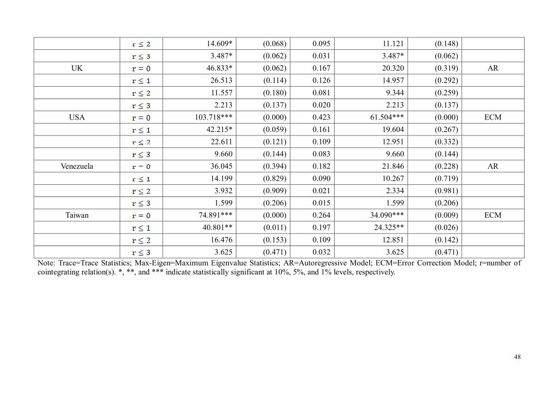
48

14.609* (0.068) 0.095 11.121 (0.148)

3.487* (0.062) 0.031 3.487* (0.062)

UK 46.833* (0.062) 0.167 20.320 (0.319) AR

26.513 (0.114) 0.126 14.957 (0.292)

11.557 (0.180) 0.081 9.344 (0.259)

2.213 (0.137) 0.020 2.213 (0.137)

USA 103.718*** (0.000) 0.423 61.504*** (0.000) ECM

42.215* (0.059) 0.161 19.604 (0.267)

22.611 (0.121) 0.109 12.951 (0.332)

9.660 (0.144) 0.083 9.660 (0.144)

Venezuela 36.045 (0.394) 0.182 21.846 (0.228) AR

14.199 (0.829) 0.090 10.267 (0.719)

3.932 (0.909) 0.021 2.334 (0.981)

1.599 (0.206) 0.015 1.599 (0.206)

Taiwan 74.891*** (0.000) 0.264 34.090*** (0.009) ECM

40.801** (0.011) 0.197 24.325** (0.026)

16.476 (0.153) 0.109 12.851 (0.142)

3.625 (0.471) 0.032 3.625 (0.471)

Note: Trace=Trace Statistics; Max-Eigen=Maximum Eigenvalue Statistics; AR=Autoregressive Model; ECM=Error Correction Model; r=number of cointegrating relation(s). *, **, and *** indicate statistically significant at 10%, 5%, and 1% levels, respectively.

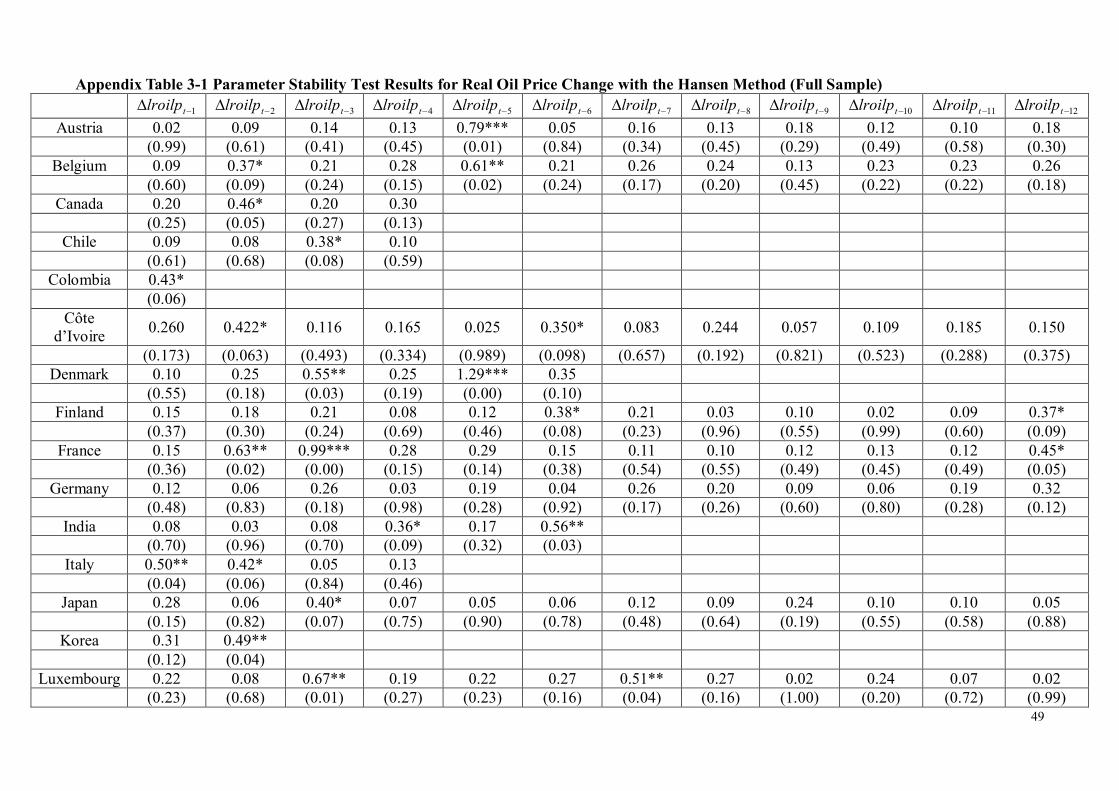
49

Appendix Table 3-1 Parameter Stability Test Results for Real Oil Price Change with the Hansen Method (Full Sample)

1 tlroilp 2 tlroilp 3 tlroilp 4 tlroilp 5 tlroilp 6 tlroilp 7 tlroilp 8 tlroilp 9 tlroilp 10 tlroilp 11 tlroilp 12 tlroilp

Austria 0.02 0.09 0.14 0.13 0.79*** 0.05 0.16 0.13 0.18 0.12 0.10 0.18 (0.99) (0.61) (0.41) (0.45) (0.01) (0.84) (0.34) (0.45) (0.29) (0.49) (0.58) (0.30)

Belgium 0.09 0.37* 0.21 0.28 0.61** 0.21 0.26 0.24 0.13 0.23 0.23 0.26 (0.60) (0.09) (0.24) (0.15) (0.02) (0.24) (0.17) (0.20) (0.45) (0.22) (0.22) (0.18)

Canada 0.20 0.46* 0.20 0.30 (0.25) (0.05) (0.27) (0.13)

Chile 0.09 0.08 0.38* 0.10 (0.61) (0.68) (0.08) (0.59)

Colombia 0.43* (0.06)

Côte d’Ivoire

0.260 0.422* 0.116 0.165 0.025 0.350* 0.083 0.244 0.057 0.109 0.185 0.150

(0.173) (0.063) (0.493) (0.334) (0.989) (0.098) (0.657) (0.192) (0.821) (0.523) (0.288) (0.375) Denmark 0.10 0.25 0.55** 0.25 1.29*** 0.35

(0.55) (0.18) (0.03) (0.19) (0.00) (0.10) Finland 0.15 0.18 0.21 0.08 0.12 0.38* 0.21 0.03 0.10 0.02 0.09 0.37*

(0.37) (0.30) (0.24) (0.69) (0.46) (0.08) (0.23) (0.96) (0.55) (0.99) (0.60) (0.09) France 0.15 0.63** 0.99*** 0.28 0.29 0.15 0.11 0.10 0.12 0.13 0.12 0.45*

(0.36) (0.02) (0.00) (0.15) (0.14) (0.38) (0.54) (0.55) (0.49) (0.45) (0.49) (0.05) Germany 0.12 0.06 0.26 0.03 0.19 0.04 0.26 0.20 0.09 0.06 0.19 0.32

(0.48) (0.83) (0.18) (0.98) (0.28) (0.92) (0.17) (0.26) (0.60) (0.80) (0.28) (0.12) India 0.08 0.03 0.08 0.36* 0.17 0.56**

(0.70) (0.96) (0.70) (0.09) (0.32) (0.03) Italy 0.50** 0.42* 0.05 0.13

(0.04) (0.06) (0.84) (0.46) Japan 0.28 0.06 0.40* 0.07 0.05 0.06 0.12 0.09 0.24 0.10 0.10 0.05

(0.15) (0.82) (0.07) (0.75) (0.90) (0.78) (0.48) (0.64) (0.19) (0.55) (0.58) (0.88) Korea 0.31 0.49**

(0.12) (0.04) Luxembourg 0.22 0.08 0.67** 0.19 0.22 0.27 0.51** 0.27 0.02 0.24 0.07 0.02

(0.23) (0.68) (0.01) (0.27) (0.23) (0.16) (0.04) (0.16) (1.00) (0.20) (0.72) (0.99)

50

Malaysia 0.63** 0.32 0.07 0.16 0.69** 0.12 0.10 0.06 (0.02) (0.11) (0.74) (0.36) (0.01) (0.48) (0.56) (0.82)

Mexico 0.05 0.03 0.10 0.19 (0.86) (0.99) (0.56) (0.28)

Netherlands 0.06 (0.79)

Nigeria 0.65** 0.21 (0.02) (0.25)

Norway 0.13 0.11 0.09 0.39* 0.03 0.18 0.15 0.06 0.23 0.06 0.03 0.70** (0.44) (0.50) (0.63) (0.08) (0.97) (0.30) (0.39) (0.78) (0.22) (0.80) (0.97) (0.01)

Portugal 0.48** (0.04)

South Africa 0.12 0.04 0.07 0.03 0.18 0.05 0.08 0.07 0.12 (0.48) (0.95) (0.71) (0.97) (0.29) (0.87) (0.70) (0.72) (0.47)

Spain 0.47* 0.12 0.08 0.10 0.20 0.04 0.45* 0.08 0.05 0.32 0.10 0.08 (0.05) (0.49) (0.67) (0.55) (0.26) (0.94) (0.05) (0.67) (0.86) (0.12) (0.58) (0.67)

Sweden 0.16 0.06 0.06 0.04 0.11 0.11 0.03 0.08 0.17 0.17 0.05 0.03 (0.35) (0.80) (0.80) (0.95) (0.52) (0.50) (0.97) (0.67) (0.32) (0.33) (0.87) (0.99)

Trinidad & Tobago

0.05 0.11 0.06 0.22 0.07 0.09

(0.86) (0.51) (0.81) (0.22) (0.72) (0.64) UK 0.30 0.26 0.25 0.04 0.55** 0.12 0.80** 0.04 0.07 0.18 0.16 0.57**

(0.13) (0.17) (0.19) (0.94) (0.03) (0.49) (0.01) (0.95) (0.72) (0.29) (0.36) (0.03) USA 0.13 0.20 0.09 0.50** 0.23 0.07 0.12 0.28 0.55** 0.24 0.31 0.02

(0.44) (0.26) (0.60) (0.04) (0.21) (0.75) (0.49) (0.15) (0.03) (0.20) (0.12) (0.99) Venezuela 0.07 0.21 0.09 0.03 0.12

(0.75) (0.24) (0.62) (0.96) (0.49) Taiwan 0.17 0.25 0.59**

(0.33) (0.18) (0.02) Note: We select the optimal lag length by minimizing the Akaike Information Criterion (AIC). Numbers in the table are test statistics and the corresponding p-values are in the parentheses. *, **, and *** indicate statistically significant unstable estimates at 10%, 5%, and 1% levels, respectively. In this paper, we use the unstable oil price change as asymmetrical variable, i.e., the positive and negative oil price changes.

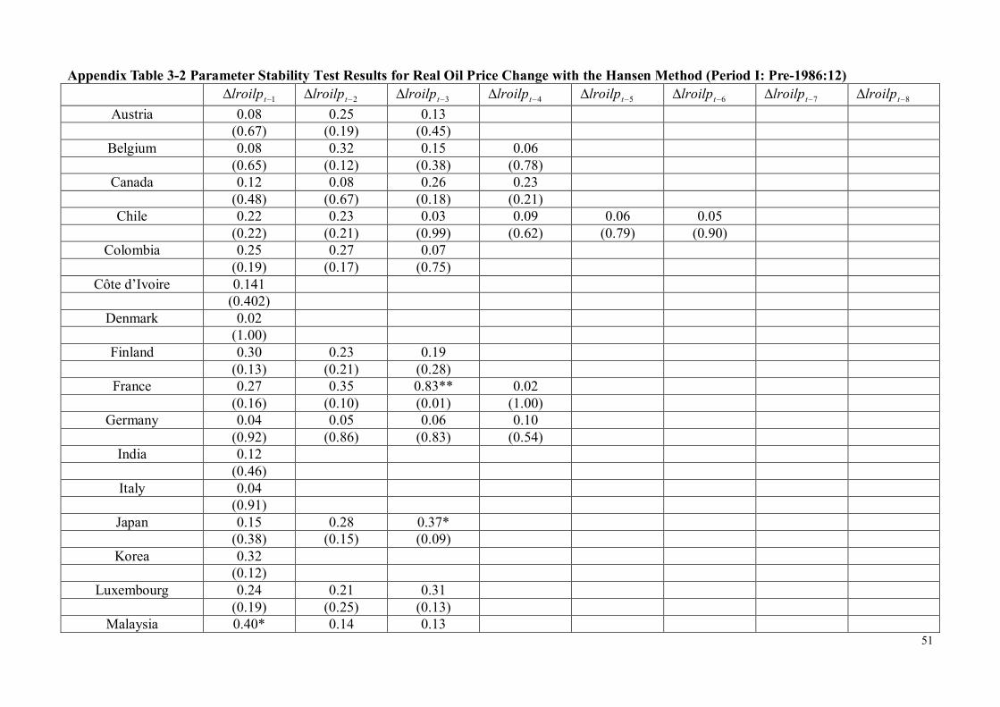
51

Appendix Table 3-2 Parameter Stability Test Results for Real Oil Price Change with the Hansen Method (Period I: Pre-1986:12)

1 tlroilp 2 tlroilp 3 tlroilp 4 tlroilp 5 tlroilp 6 tlroilp 7 tlroilp 8 tlroilp

Austria 0.08 0.25 0.13 (0.67) (0.19) (0.45)

Belgium 0.08 0.32 0.15 0.06 (0.65) (0.12) (0.38) (0.78)

Canada 0.12 0.08 0.26 0.23 (0.48) (0.67) (0.18) (0.21)

Chile 0.22 0.23 0.03 0.09 0.06 0.05 (0.22) (0.21) (0.99) (0.62) (0.79) (0.90)

Colombia 0.25 0.27 0.07 (0.19) (0.17) (0.75)

Côte d’Ivoire 0.141 (0.402)

Denmark 0.02 (1.00)

Finland 0.30 0.23 0.19 (0.13) (0.21) (0.28)

France 0.27 0.35 0.83** 0.02 (0.16) (0.10) (0.01) (1.00)

Germany 0.04 0.05 0.06 0.10 (0.92) (0.86) (0.83) (0.54)

India 0.12 (0.46)

Italy 0.04 (0.91)

Japan 0.15 0.28 0.37* (0.38) (0.15) (0.09)

Korea 0.32 (0.12)

Luxembourg 0.24 0.21 0.31 (0.19) (0.25) (0.13)

Malaysia 0.40* 0.14 0.13

52

(0.07) (0.39) (0.44) Mexico 0.16 0.05 0.03 0.14 0.10 0.09 0.06

(0.34) (0.87) (0.97) (0.39) (0.58) (0.61) (0.83) Netherlands 0.10

(0.56) Nigeria 0.18 0.22 0.23

(0.31) (0.23) (0.21) Norway 0.27

(0.16) Portugal 0.51**

(0.04) South Africa 0.20 0.09 0.06 0.02 0.12 0.28 0.10 0.07

(0.25) (0.62) (0.78) (0.99) (0.46) (0.16) (0.59) (0.77) Spain 0.56**

(0.03) Sweden 0.17 0.05 0.06

(0.31) (0.88) (0.81) Trinidad & Tobago 0.02 0.28 0.03

(0.99) (0.15) (0.96) UK 0.12 0.09 0.17

(0.49) (0.63) (0.32) USA 0.35 0.11 0.11 0.20 0.03 0.10 0.19 0.05

(0.10) (0.53) (0.53) (0.26) (0.96) (0.55) (0.27) (0.84) Venezuela 0.23 0.22 0.07 0.15 0.21 0.19

(0.21) (0.23) (0.72) (0.36) (0.25) (0.29) Taiwan 0.27 0.26 0.05

(0.16) (0.17) (0.87) Note: We select the optimal lag length by minimizing the Akaike Information Criterion (AIC). Numbers in the table are test statistics and the corresponding p-values are in the parentheses. *, **, and *** indicate statistically significant unstable estimates at 10%, 5%, and 1% levels, respectively. In this paper, we use the unstable oil price change as asymmetrical variable, i.e., the positive and negative oil price changes.

53

Appendix Table 3-3 Stability Test Results for Real Oil Price Change Parameter with the Hansen Method (Period II: 1987:01~1998:12)

1 tlroilp 2 tlroilp 3 tlroilp 4 tlroilp 5 tlroilp 6 tlroilp 7 tlroilp 8 tlroilp 9 tlroilp 10 tlroilp

Austria 0.07 0.58** 0.10 0.11 0.12 (0.75) (0.03) (0.56) (0.52) (0.49)

Belgium 0.10 (0.56)

Canada 0.09 0.03 (0.65) (0.99)

Chile 0.11 0.06 0.13 0.30 (0.52) (0.83) (0.44) (0.13)

Colombia 0.07 (0.72)

Côte d’Ivoire

0.148 0.276 0.262 0.194 0.045 0.428* 0.254 0.243 0.035 0.586**

(0.382) (0.155) (0.170) (0.271) (0.898) (0.061) (0.180) (0.193) (0.955) (0.024) Denmark 0.07 0.08 0.05 0.30 0.03 0.34

(0.73) (0.65) (0.85) (0.14) (0.99) (0.11) Finland 0.07

(0.75) France 0.07 0.06

(0.75) (0.84) Germany 0.27

(0.16) India 0.32

(0.12) Italy 0.12 0.04 0.24 0.20 0.07 0.17 0.17

(0.48) (0.92) (0.20) (0.26) (0.77) (0.33) (0.31) Japan 0.04 0.13 0.26 0.10

(0.93) (0.43) (0.17) (0.55) Korea 0.05 0.08

(0.84) (0.67) Luxembourg 0.06

(0.77)

54

Malaysia 0.04 0.06 0.17 0.07 0.08 0.06 0.23 0.08 0.05 (0.93) (0.83) (0.33) (0.76) (0.69) (0.78) (0.22) (0.65) (0.86)

Mexico 0.06 0.14 0.02 (0.82) (0.40) (0.99)

Netherlands 0.25 0.15 0.13 (0.19) (0.37) (0.43)

Nigeria 0.06 (0.81)

Norway 0.06 0.25 0.07 0.34 0.18 0.03 (0.82) (0.18) (0.71) (0.10) (0.29) (0.96)

Portugal 0.04 (0.91)

South Africa 0.19 0.13 (0.27) (0.46)

Spain 0.07 0.05 0.16 0.04 0.05 0.16 (0.71) (0.88) (0.35) (0.91) (0.89) (0.34)

Sweden 0.06 0.05 0.08 0.04 0.13 (0.77) (0.85) (0.71) (0.94) (0.45)

Trinidad & Tobago

0.12

(0.49) UK 0.03 0.03 0.38* 0.11

(0.96) (0.98) (0.08) (0.53) USA 0.18 0.05 0.14 0.05 0.03 0.08 0.04

(0.31) (0.84) (0.42) (0.89) (0.96) (0.68) (0.92) Venezuela 0.41* 0.20 0.14 0.03 0.12

(0.07) (0.26) (0.40) (0.96) (0.46) Taiwan 0.05 0.37* 0.18 0.07

(0.88) (0.09) (0.29) (0.76) Note: We select the optimal lag length by minimizing the Akaike Information Criterion (AIC). Numbers in the table are test statistics and the corresponding p-values are in the parentheses. *, **, and *** indicate statistically significant unstable estimates at 10%, 5%, and 1% levels, respectively. In this paper, we use the unstable oil price change as asymmetrical variable, i.e., the positive and negative oil price changes.

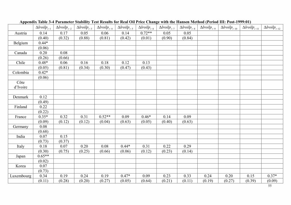
55

Appendix Table 3-4 Parameter Stability Test Results for Real Oil Price Change with the Hansen Method (Period III: Post-1999:01)

1 tlroilp 2 tlroilp 3 tlroilp 4 tlroilp 5 tlroilp 6 tlroilp 7 tlroilp 8 tlroilp 9 tlroilp 10 tlroilp 11 tlroilp 12 tlroilp

Austria 0.14 0.17 0.05 0.06 0.14 0.72** 0.05 0.05 (0.40) (0.32) (0.88) (0.81) (0.42) (0.01) (0.90) (0.84)

Belgium 0.44* (0.06)

Canada 0.20 0.08 (0.26) (0.66)

Chile 0.48* 0.06 0.16 0.18 0.12 0.13 (0.05) (0.81) (0.34) (0.30) (0.47) (0.43)

Colombia 0.42* (0.06)

Côte d’Ivoire

Denmark 0.12

(0.49) Finland 0.22

(0.22) France 0.35* 0.32 0.31 0.52** 0.09 0.46* 0.14 0.09

(0.09) (0.12) (0.12) (0.04) (0.63) (0.05) (0.40) (0.63) Germany 0.08

(0.68) India 0.07 0.15

(0.73) (0.37) Italy 0.18 0.07 0.20 0.08 0.44* 0.31 0.22 0.29

(0.30) (0.75) (0.25) (0.66) (0.06) (0.12) (0.23) (0.14) Japan 0.65**

(0.02) Korea 0.07

(0.73) Luxembourg 0.34 0.19 0.24 0.19 0.47* 0.09 0.23 0.33 0.24 0.20 0.15 0.37*

(0.11) (0.28) (0.20) (0.27) (0.05) (0.64) (0.21) (0.11) (0.19) (0.27) (0.39) (0.09)

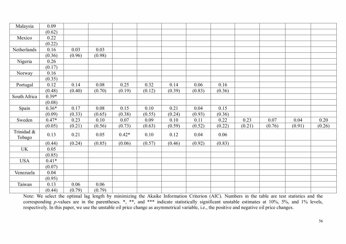
56

Malaysia 0.09 (0.62)

Mexico 0.22 (0.22)

Netherlands 0.16 0.03 0.03 (0.36) (0.96) (0.98)

Nigeria 0.26 (0.17)

Norway 0.16 (0.35)

Portugal 0.12 0.14 0.08 0.25 0.32 0.14 0.06 0.16 (0.48) (0.40) (0.70) (0.19) (0.12) (0.39) (0.83) (0.36)

South Africa 0.39* (0.08)

Spain 0.36* 0.17 0.08 0.15 0.10 0.21 0.04 0.15 (0.09) (0.33) (0.65) (0.38) (0.55) (0.24) (0.93) (0.36)

Sweden 0.47* 0.23 0.10 0.07 0.09 0.10 0.11 0.22 0.23 0.07 0.04 0.20 (0.05) (0.21) (0.56) (0.73) (0.63) (0.59) (0.52) (0.22) (0.21) (0.76) (0.91) (0.26)

Trinidad & Tobago

0.13 0.21 0.05 0.42* 0.10 0.12 0.04 0.06

(0.44) (0.24) (0.85) (0.06) (0.57) (0.46) (0.92) (0.83) UK 0.05

(0.85) USA 0.41*

(0.07) Venezuela 0.04

(0.95) Taiwan 0.13 0.06 0.06

(0.44) (0.79) (0.79) Note: We select the optimal lag length by minimizing the Akaike Information Criterion (AIC). Numbers in the table are test statistics and the corresponding p-values are in the parentheses. *, **, and *** indicate statistically significant unstable estimates at 10%, 5%, and 1% levels, respectively. In this paper, we use the unstable oil price change as asymmetrical variable, i.e., the positive and negative oil price changes.

57

Appendix Table 4 Estimated Coefficients for Consumer Price Change Equations

Current Lagged Periods Total Impact

p Symmetry Asymmetry

Austria All 12 Positive Negative

Coef. 0.003 0.004 0.006*** -0.001 0.009 0.003 t-Stat. (1.279) (1.227) (2.689) (-0.198)

I 3

Coef. 0.001 0.001 t-Stat. (0.225)

II 5

Coef. 0.007 -0.014* 0.008 -0.010 0.015 -0.023 t-Stat. (1.138) (-1.802) (1.234) (-1.312)

III 8

Coef. 0.009** 0.009 -0.004 -0.010** 0.006 -0.001 t-Stat. (2.157) (1.623) (-0.790) (-2.226)

Belgium All 12

Coef. 0.006*** 0.013*** 0.001 -0.002 0.006** -0.002 0.013 0.009 t-Stat. (2.630) (4.210) (0.396) (-0.794) (2.465) (-0.779)

I 4

Coef. 0.003 0.003 t-Stat. (1.071)

II 1

Coef. 0.010*** 0.010 t-Stat. (3.637)

III 1

Coef. 0.020*** 0.011* 0.009* 0.005 0.029 0.016 t-Stat. (3.638) (1.951) (1.723) (0.891)

Canada All 4

Coef. 0.003 0.007** 0.006** -0.008** 0.009 -0.001 t-Stat. (1.374) (2.000) (2.441) (-2.220)

58

I 4 0.001

Coef. 0.000 -0.004* 0.005* t-Stat. (0.133) (-1.680) (1.909)

II 2

Coef. -0.003 -0.003 t-Stat. (-1.027)

III 2

Coef. 0.022*** 0.015*** -0.008* 0.029 t-Stat. (6.193) (3.714) (-1.894)

Chile All 4

Coef. 0.004 -0.013 0.008 -0.002 0.012 -0.015 t-Stat. (0.372) (-1.064) (0.667) (-0.160)

I 6

Coef. -0.024 0.027* 0.003 t-Stat. (-1.489) (1.701)

II 4

Coef. 0.017** 0.014* -0.012* 0.019 t-Stat. (2.409) (1.956) (-1.742)

III 6

Coef. 0.017*** 0.013** 0.013** 0.018*** 0.030 0.031 t-Stat. (3.016) (2.084) (2.235) (2.828)

Colombia All 1

Coef. 0.010 -0.047*** 0.011 -0.005 0.021 -0.052 t-Stat. (1.372) (-4.792) (1.517) (-0.461)

I 3

Coef. -0.013 -0.013 t-Stat. (-1.620)

II 1

Coef. -0.008 -0.008 t-Stat. (-1.057)

59

III 1

Coef. -0.004 -0.005 0.013 -0.006 0.009 -0.011 t-Stat. (-0.427) (-0.679) (1.605) (-0.785)

Côte d’Ivoire

All 12

Coef. -0.020 -0.106*** 0.022* -0.026 0.002 -0.132 t-Stat. (-1.547) (-5.882) (1.698) (-1.447)

I 1

Coef. -0.081*** 0.032* -0.049 t-Stat. (-4.772) (1.778)

II 12

Coef. 0.005 -0.039** 0.002 0.014 0.025** -0.004 0.032 -0.029 t-Stat. (0.402) (-2.527) (0.149) (0.891) (2.237) (-0.311)

III 1

Coef. -0.006 -0.006 t-Stat. (-0.782)

Denmark All 7

Coef. 0.006* 0.009* 0.002 -0.007 0.008** -0.003 0.016 -0.001 t-Stat. (1.661) (1.701) (0.554) (-1.275) (2.244) (-0.626)

I 1

Coef. 0.002 0.002 t-Stat. (0.320)

II 6

Coef. 0.008*** 0.009*** -0.012*** -0.008** -0.003 t-Stat. (2.731) (2.841) (-3.963) (-2.584)

III 1

Coef. 0.010** 0.013*** 0.023 t-Stat. (2.331) (2.811)

Finland All 12

Coef. 0.003 0.000 0.007* 0.005 0.007** 0.001 0.017 0.006

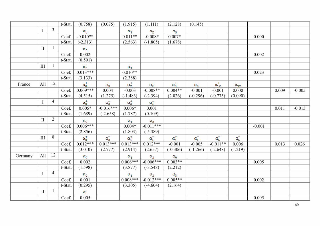
60

t-Stat. (0.758) (0.075) (1.915) (1.111) (2.128) (0.145)

I 3

Coef. -0.010** 0.011** -0.008* 0.007* 0.000 t-Stat. (-2.313) (2.563) (-1.805) (1.678)

II 1

Coef. 0.002 0.002 t-Stat. (0.591)

III 1

Coef. 0.013*** 0.010** 0.023 t-Stat. (3.133) (2.388)

France All 12

Coef. 0.009*** 0.004 -0.003 -0.008** 0.004** -0.001 -0.001 0.000 0.009 -0.005 t-Stat. (4.515) (1.275) (-1.483) (-2.394) (2.026) (-0.296) (-0.773) (0.090)

I 4

Coef. 0.005* -0.016*** 0.006* 0.001 0.011 -0.015 t-Stat. (1.689) (-2.658) (1.787) (0.109)

II 2

Coef. 0.006*** 0.004* -0.011*** -0.001 t-Stat. (2.856) (1.803) (-5.389)

III 8

Coef. 0.012*** 0.013*** 0.013*** 0.012*** -0.001 -0.005 -0.011** 0.006 0.013 0.026 t-Stat. (3.010) (2.777) (2.914) (2.657) (-0.306) (-1.266) (-2.648) (1.219)

Germany All 12

Coef. 0.002 0.006*** -0.006*** 0.003** 0.005 t-Stat. (1.598) (3.877) (-3.548) (2.212)

I 4

Coef. 0.001 0.008*** -0.012*** 0.005** 0.002 t-Stat. (0.295) (3.305) (-4.604) (2.164)

II 1

Coef. 0.005 0.005

61

t-Stat. (1.395)

III 1

Coef. 0.010** 0.008** 0.018 t-Stat. (2.508) (2.010)

India All 6

Coef. -0.003 -0.026*** 0.010 -0.020** 0.011* 0.001 0.018 -0.045 t-Stat. (-0.417) (-2.896) (1.551) (-2.212) (1.737) (0.097)

I 1

Coef. -0.016** 0.009 -0.007 t-Stat. (-2.085) (1.213)

II 1

Coef. -0.023** 0.021** -0.002 t-Stat. (-2.509) (2.230)

III 2

Coef. 0.002 0.008 0.015* 0.025 t-Stat. (0.251) (1.070) (1.942)

Italy All 4

Coef. 0.001 0.003 0.007*** 0.003 0.002 -0.006 0.010 0.000 t-Stat. (0.577) (0.852) (2.667) (0.831) (0.894) (-1.626)

I 1

Coef. 0.002 0.008** 0.010 t-Stat. (0.484) (2.375)

II 7

Coef. 0.003* -0.004** -0.001 t-Stat. (1.738) (-2.123)

III 8

Coef. 0.003 0.005* -0.002 -0.001 0.001 0.004 t-Stat. (1.098) (1.878) (-0.833) (-0.430)

Japan All 12

Coef. 0.006 -0.011* 0.009** 0.006 0.015 -0.005

62

t-Stat. (1.371) (-1.759) (2.076) (0.961)

I 3

Coef. 0.007 -0.043*** 0.012 0.001 0.019 -0.042 t-Stat. (0.941) (-3.263) (1.540) (0.071)

II 4

Coef. 0.003 0.003 t-Stat. (0.564)

III 1

Coef. -0.001 0.001 0.005 0.009 0.004 0.010 t-Stat. (-0.107) (0.142) (1.018) (1.640)

Korea All 2

Coef. 0.014*** -0.011 -0.005 -0.014* 0.009 -0.025 t-Stat. (2.720) (-1.583) (-0.965) (-1.940)

I 1

Coef. 0.011 0.017** 0.028 t-Stat. (1.520) (2.382)

II 2

Coef. -0.003 -0.002 -0.002 -0.007 t-Stat. (-0.472) (-0.397) (-0.344)

III 1

Coef. 0.012** 0.010** 0.022 t-Stat. (2.489) (2.026)

Luxembourg All 12

Coef. 0.003 0.005 0.006** -0.001 -0.004 -0.003 0.005 0.001 t-Stat. (1.071) (1.362) (2.293) (-0.330) (-1.405) (-0.710)

I 3

Coef. 0.001 0.014*** -0.011*** 0.004 0.008 t-Stat. (0.458) (5.116) (-3.769) (1.289)

II 1

Coef. 0.002 0.006** 0.008

63

t-Stat. (0.925) (2.573)

III 12

Coef. -0.002 0.015*** 0.009 -0.009 0.006 -0.001 0.013 0.005 t-Stat. (-0.352) (2.680) (1.579) (-1.517) (1.048) (-0.140)

Malaysia All 8

Coef. -0.002 -0.011** 0.012*** 0.001 -0.006* 0.001 0.004 -0.009 t-Stat. (-0.589) (-2.180) (3.537) (0.102) (-1.833) (0.294)

I 3

Coef. 0.003 -0.016 0.020*** 0.006 0.023 -0.010 t-Stat. (0.511) (-1.233) (3.568) (0.508)

II 9

Coef. -0.013*** 0.007* -0.006 t-Stat. (-3.590) (1.890)

III 1

Coef. 0.001 0.001 0.002 t-Stat. (0.403) (0.415)

Mexico All 4

Coef. -0.010** 0.012** 0.002 t-Stat. (-2.028) (2.483)

I 7

Coef. -0.005 -0.005 t-Stat. (-0.810)

II 3

Coef. -0.008 0.018* 0.010 t-Stat. (-0.761) (1.847)

III 1

Coef. 0.001 0.012*** 0.013 t-Stat. (0.336) (3.240)

Netherlands All 1

Coef. -0.019*** -0.019

64

t-Stat. (-2.642)

I 1

Coef. -0.028*** -0.028 t-Stat. (-2.804)

II 3

Coef. -0.021 -0.021 t-Stat. (-1.129)

III 3

Coef. 0.016*** 0.016 t-Stat. (3.602)

Nigeria All 2

Coef. -0.008 -0.165*** 0.009 0.012 0.001 -0.153 t-Stat. (-0.534) (-7.892) (0.585) (0.552)

I 3

Coef. -0.074*** 0.037** -0.037 t-Stat. (-4.539) (2.209)

II 1

Coef. -0.075*** -0.075 t-Stat. (-3.194)

III 1

Coef. -0.045* -0.045 t-Stat. (-1.825)

Norway All 12

Coef. 0.004 0.002 -0.004 0.004 0.007** -0.007* 0.007 -0.001 t-Stat. (1.488) (0.380) (-1.514) (0.887) (2.569) (-1.751)

I 1

Coef. -0.005 -0.005 t-Stat. (-1.215)

II 6

Coef. -0.003 0.009** -0.007* -0.006* 0.012*** 0.005

65

t-Stat. (-0.971) (2.585) (-1.947) (-1.684) (3.258)

III 1

Coef. 0.012** 0.012 t-Stat. (2.020)

Portugal All 1

Coef. 0.002 -0.043*** 0.021*** 0.009 0.023 -0.034 t-Stat. (0.238) (-3.953) (2.856) (0.827)

I 1

Coef. 0.009 -0.120*** 0.026** 0.054** 0.035 -0.066 t-Stat. (0.736) (-4.668) (2.143) (2.050)

II 1

Coef. 0.001 0.001 t-Stat. (0.260)

III 8

Coef. -0.002 0.009*** 0.007 t-Stat. (-0.482) (2.683)

South Africa All 9

Coef. -0.006** 0.009*** 0.003 t-Stat. (-2.195) (2.899)

I 8

Coef. -0.016*** 0.012** -0.004 t-Stat. (-3.443) (2.545)

II 2

Coef. 0.010** 0.010 t-Stat. (2.105)

III 1

Coef. 0.016* 0.001 0.034*** 0.005 0.050 0.006 t-Stat. (1.797) (0.089) (3.973) (0.605)

Spain All 12

Coef. 0.001 0.001 0.007 0.001 0.002 0.004 0.010 0.006

66

t-Stat. (0.158) (0.090) (1.477) (0.252) (0.453) (0.744)

I 1

Coef. -0.007 -0.033** -0.004 0.014 -0.011 -0.019 t-Stat. (-0.586) (-2.247) (-0.305) (0.967)

II 6

Coef. 0.006 0.006 t-Stat. (1.593)

III 8

Coef. 0.020*** 0.004 0.012** 0.014** 0.032 0.018 t-Stat. (3.673) (0.740) (2.166) (2.365)

Sweden All 12

Coef. 0.001 0.006** 0.007*** -0.005* 0.005* 0.014 t-Stat. (0.449) (2.305) (2.649) (-1.699) (1.903)

I 3

Coef. -0.004 0.008* 0.004 t-Stat. (-0.851) (1.904)

II 5

Coef. 0.007 0.010* 0.017 t-Stat. (1.123) (1.678)

III 12

Coef. 0.007 0.020*** 0.007 -0.008 0.014 0.012 t-Stat. (1.351) (3.718) (1.382) (-1.433)

Trinidad and Tobago

All 6

Coef. -0.008* 0.005 0.008* 0.005 t-Stat. (-1.864) (1.126) (1.799)

I 3

Coef. -0.028*** -0.028 t-Stat. (-3.645)

II 1

67

Coef. -0.001 -0.001 t-Stat. (-0.116)

III 8

Coef. 0.020** -0.045*** 0.023** 0.011 0.043 -0.034 t-Stat. (2.040) (-4.530) (2.487) (1.128)

UK All 12

Coef. 0.008** -0.004 0.009*** 0.000 -0.010*** 0.012** 0.008** -0.001 0.015 0.007 t-Stat. (2.273) (-0.911) (2.719) (0.080) (-2.956) (2.380) (2.375) (-0.148)

I 3

Coef. 0.008 -0.025** -0.001 -0.004 0.007 -0.029 t-Stat. (1.410) (-2.307) (-0.228) (-0.342)

II 4

Coef. 0.017** -0.005 0.006 -0.003 0.023 -0.008 t-Stat. (2.063) (-0.588) (0.856) (-0.374)

III 1

Coef. 0.006 0.015*** 0.021 t-Stat. (1.338) (3.308)

USA All 12

Coef. 0.007*** 0.016*** 0.005*** -0.004* 0.000 -0.001 0.012 0.011 t-Stat. (4.335) (7.017) (3.034) (-1.738) (0.188) (-0.268)

I 8

Coef. 0.005*** 0.007*** -0.005*** -0.004** 0.004** 0.005*** 0.012 t-Stat. (2.956) (4.069) (-2.740) (-2.424) (2.079) (2.728)

II 7

Coef. 0.007*** 0.005*** -0.006*** 0.006 t-Stat. (3.787) (2.775) (-3.347)

III 1

Coef. 0.025*** 0.019*** 0.015** 0.009 0.040 0.028 t-Stat. (4.473) (3.000) (2.582) (1.473)

Venezuela All 5

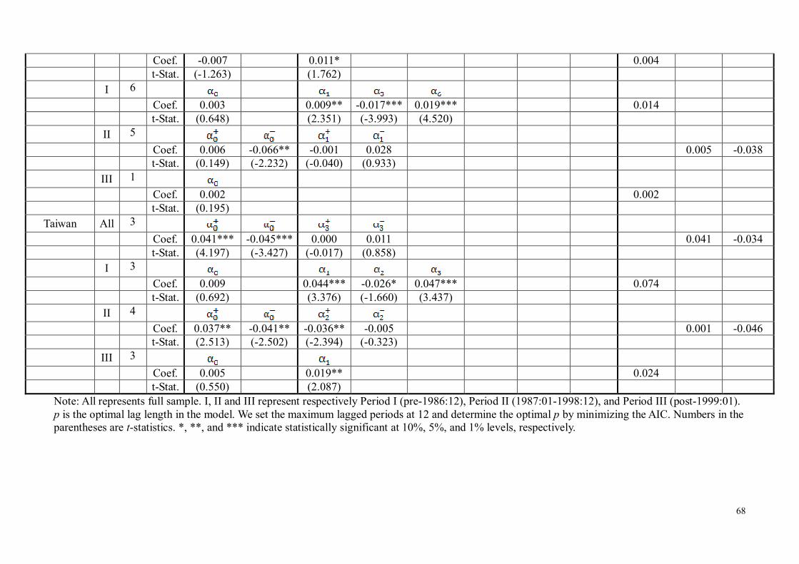
68

Coef. -0.007 0.011* 0.004 t-Stat. (-1.263) (1.762)

I 6

Coef. 0.003 0.009** -0.017*** 0.019*** 0.014 t-Stat. (0.648) (2.351) (-3.993) (4.520)

II 5

Coef. 0.006 -0.066** -0.001 0.028 0.005 -0.038 t-Stat. (0.149) (-2.232) (-0.040) (0.933)

III 1

Coef. 0.002 0.002 t-Stat. (0.195)

Taiwan All 3

Coef. 0.041*** -0.045*** 0.000 0.011 0.041 -0.034 t-Stat. (4.197) (-3.427) (-0.017) (0.858)

I 3

Coef. 0.009 0.044*** -0.026* 0.047*** 0.074 t-Stat. (0.692) (3.376) (-1.660) (3.437)

II 4

Coef. 0.037** -0.041** -0.036** -0.005 0.001 -0.046 t-Stat. (2.513) (-2.502) (-2.394) (-0.323)

III 3

Coef. 0.005 0.019** 0.024 t-Stat. (0.550) (2.087)

Note: All represents full sample. I, II and III represent respectively Period I (pre-1986:12), Period II (1987:01-1998:12), and Period III (post-1999:01). p is the optimal lag length in the model. We set the maximum lagged periods at 12 and determine the optimal p by minimizing the AIC. Numbers in the parentheses are t-statistics. *, **, and *** indicate statistically significant at 10%, 5%, and 1% levels, respectively.