1

Analysis of Variance with Unbalanced Data: An Update for Ecology & Evolution 1

Andy Hector, Stefanie von Felten and Bernhard Schmid 2

3

Institute of Environmental Sciences, University of Zurich, Winterthurerstrasse 190, CH-4

8057 Zurich, Switzerland 5

6

Corresponding author: 7

Andy Hector 8

Email: ahector@uwinst.uzh.ch 9

Phone: +41 (0)44 635 48 04 10

Fax: +41 ( 0)44 635 57 11 11

12

2

Abstract 1

Factorial analysis of variance (ANOVA) with unbalanced (non-orthogonal) data is a 2

commonplace but controversial and poorly understood topic in applied statistics. We explain 3

that ANOVA calculates the sum of squares for each term in the model formula sequentially 4

(type I sums of squares) and show how ANOVA tables of adjusted sums of squares are 5

composite tables assembled from multiple sequential analyses. A different ANOVA is 6

performed for each explanatory variable or interaction so that each term is placed last in the 7

model formula in turn and adjusted for the others. The sum of squares for each term in the 8

analysis can be calculated after adjusting only for the main effects of other explanatory 9

variables (type II sums of squares) or, controversially, for both main effects and interactions 10

(type III sums of squares). We summarize the main recent developments and emphasize the 11

shift away from the search for the ‘right’ ANOVA table in favour of presenting one or more 12

models that best suit the objectives of the analysis. 13

14

Keywords: Adjusted sums of squares; Type III sums of squares; ANOVA; Orthogonality; 15

Linear models; R. 16

17

3

Introduction 1

Analysis of variance (ANOVA) continues to be one of the most widely used forms of 2

statistical analysis in many areas of science (Gelman, 2005, Gelman and Hill, 2007). 3

Nevertheless, factorial ANOVA with unbalanced (non-orthogonal – supplement S1) data is a 4

controversial topic in applied statistics and one of the areas of ANOVA that is most poorly 5

understood in ecology, evolution and environmental science. This is partly because bio-6

statistics textbooks appear to avoid the topic, perhaps because it is controversial. The last 7

coverage of the topic in the ecology and evolution journals revealed disagreement on how to 8

best approach ANOVA of unbalanced data (Shaw and Mitchell-Olds, 1993, Stewart-Oaten, 9

1995). There still appears to be no consensus within the statistical community, but there has 10

been further discussion that has yet to make its way into the ecology and evolution literature. 11

There has also been a move away from finding the ‘right’ ANOVA table towards presenting 12

the one or more models that best match the objectives of the analysis. 13

In this paper, we give non-technical explanations of the issues involved in ANOVA of 14

unbalanced data, particularly the different types of adjusted sums of squares. We also provide 15

(as supplementary material) code for the analysis of worked examples of unbalanced 16

ANOVA designs using the open-source R language for statistical computing and graphics that 17

is fast becoming the lingua franca for analysis in ecology and evolution (R Development 18

Core Team, 2009). 19

The Problem 20

With balanced designs one factor can be held constant while the other is varied 21

independently. However, this desirable property of orthogonality is usually lost for 22

unbalanced designs (supplement S1). When explanatory variables are correlated with each 23

other due to imbalance in the number of replicates for different treatment combinations the 24

values of the sums of squares depend on the position of the factors in the ANOVA model 25

4

formula. Because ANOVA and regression are special cases of general linear models there is 1

much overlap between this topic and multiple regression. In non-orthogonal designs, some of 2

the explanatory variables (and, if present, their interactions) are positively or negatively 3

correlated with each other; that is they are partially collinear or confounded. Using a Venn 4

diagram (Figure 1), positive correlations can be illustrated as causing over-lapping and 5

negative correlations under-lapping sums of squares. The desire to find a technological fix 6

that provides a single outcome to the analysis of orthogonal and non-orthogonal data is clear. 7

In response, some statistical software companies have developed several types of adjusted 8

sums of squares. 9

Sequential and Adjusted Sums of Squares 10

The sums of squares used in ANOVA as originally proposed by Fisher (1925) are calculated 11

sequentially for each main effect and each two-way or higher-order interaction following the 12

sequence of terms at each level in the model formula. One desirable feature of sequential 13

sums of squares is that they are additive; that is the total sum of squares is decomposed into a 14

series of additive parts. The total sum of squares for a sequential ANOVA is the same for all 15

orderings of the explanatory variables in the model formula even though the values for the 16

individual variables change with their position in the sequence. 17

The alternative to sequential sums of squares is to use one of a variety of adjusted 18

(also known as partial, unique, marginal, conditional or unweighted) sums of squares. These 19

adjusted sums of squares are sometimes linked to early work by Yates (1933, 1934) as 20

discussed by Nelder & Lane (1995) and summarized in the supplement (S2). Adjusted sums 21

of squares can be divided into two categories (Herr, 1986, Macnaughton, 1998). As the name 22

implies, adjusted sums of squares are calculated for a given explanatory variable after 23

adjusting for the other variables in the statistical model formula. The different systems of 24

adjusted sums of squares can then be categorized as to whether they adjust a given variable 25

5

for the other variables at the same level (e.g. adjusting each main effect for the other main 1

effects) or whether the adjustment also includes interactions at higher levels. Macnaughton 2

(1998) has termed these ‘higher-level terms omitted (HTO)’ and ‘higher-level terms included 3

(HTI)’, while Herr (1986) termed them ‘each adjusted for other (EAD)’ and ‘standard 4

parametric (STP)’. Other terminologies exist (supplement S2) but we find Macnaughton's the 5

most transparent. 6

In the following section we express these two general classes more formally and 7

illustrate them using a simple worked example of a two-way factorial ANOVA (this is the 8

design used in most discussion of this topic in the statistical literature). To build on earlier 9

literature on this topic we use the hypothetical dataset from Shaw & Mitchell-Olds (1993). 10

The dataset (Table 1) comprises height of experimental target organisms as the response 11

variable, the experimental removal (or not) of neighbours as a first explanatory factor and the 12

initial size of the target organisms as a second factor. Both factors have two levels since initial 13

sizes are recorded only as two classes (small or large). The design is therefore a fully-factorial 14

22 design: that is two factors - each with two levels - crossed so that all four possible 15

combinations (or 'cells' in a tabular representation of the design) are present. The design is 16

unbalanced because the different combinations have different numbers of replicates but no 17

cells are empty (a more extreme form of imbalance). Because the proportional number of 18

replicates are not the same across treatments the design is non-orthogonal, that is the two 19

explanatory variables are not independent of each other. 20

Sequential Sums of Squares 21

The design can be analysed with a two-way factorial ANOVA that considers the main effects 22

of the neighbour removal treatment, the initial size class, and their interaction. Due to the 23

imbalance, the sums of squares for the main effects of the two variables change with the two 24

alternative sequential model formulas, which can be written using the effects notation as: 25

6

yijk = µ + αi + βj + γij + εink (1) 1

yijk = µ + βj+ αi + γij + εijk (2) 2

where yijk is the response (final height) of the kth organism (k = 1,2,…, nij), in the ith 3

level of factor α (the neighbour removal treatment), and the jth level of factor β (initial size), γ 4

is the interaction of the two treatments, µ indicates the intercept (here the grand mean; 5

supplement S3), and ε the within-group error. These two models can be written in the widely 6

used statistical model formula notation of Wilkinson & Rogers (1973) as follows: 7

T + S + T.S (3) 8

S + T + T.S (4) 9

where T is neighbour removal treatment, S is initial plant size and T.S the interaction 10

(which could be equivalently written as S.T). The intercept is taken as implicit in this 11

notation. The model with treatment fitted first produces the sequential ANOVA shown in 12

Table 2a and the model with initial size fitted first produces Table 2b. 13

Note that in the two sequential models the values for the interaction, residual error and 14

total sum of squares are the same, despite differences for the main effects. These differences 15

in the main effect sums of squares arise because treatment and initial size are not orthogonal. 16

When treatment is fitted before size, treatment is not significant and initial size is highly 17

significant. But when the order is reversed and initial size is put first its sum of squares is 18

reduced (although it remains highly significant) and the sum of squares for treatment is 19

increased so that it borders on being significant too (Table 2). The change of the treatment 20

effect from convincingly non-significant to marginal makes clear the dangers of sequential 21

sums of squares: fitting only one of these models could give an incomplete and potentially 22

misleading impression. The complexity of sequential sums of squares is also clear: we have 23

had to fit two models instead of one (for more complex models the numbers of alternatives 24

7

increases dramatically)? Is one correct and the other wrong? Or, are both correct but one 1

preferred over the other? 2

Adjusted Sums of Squares With Higher-Level Terms Omitted 3

The higher-level terms omitted adjusted sum of squares for the interaction can be written in 4

either of the two following ways: 5

SS(T.S | µ + T + S) (5) 6

SS(T.S | µ + S + T) (6) 7

that is, the sum of squares for the interaction conditional on (or adjusted for) all the 8

lower-order terms: the grand mean, the main effects of both neighbour removal treatment and 9

initial size. The order of the main effects does not matter since their combined value is the 10

same and therefore the sums of squares for the interaction is also the same with either 11

formulation. Similarly, the higher-level terms omitted adjusted sum of squares for treatment 12

(T) and for initial size (S) can be written, respectively, as: 13

SS(T | µ + S) (7) 14

SS(S | µ + T) (8) 15

The different models considered above (we require only 5 or 6, not both) can be 16

written in the Wilkinson & Rogers notation, respectively, as: 17

T + S + T.S (9) 18

S + T (10) 19

T + S (11) 20

Model 9, for example, can be said to fit the effect of T ignoring S and then the effect 21

of S eliminating T (McCullagh and Nelder, 1989). That is, for every variable in a sequential 22

model formula preceding variables are said to be eliminated and subsequent variables 23

ignored. The ANOVA tables for these three sequential analyses are shown in Table 3a-c. A 24

composite ANOVA table summarising these adjusted sums of squares can be assembled from 25

8

these three separate sequential models as follows. Equations 6 - 8 each specify adjusted sum 1

of squares for a single term (T.S, T and S respectively). To get these adjusted sums of squares 2

we fit models 9 – 11 (Table 3a - c). In each case we take only the sum of squares for the final 3

term (excluding the residual error, which is the same in all cases) and use these to build the 4

composite ANOVA table of adjusted sums of squares (3d). Note that the residual sum of 5

squares are the same in both cases and that if we add up the adjusted sums of squares in the 6

composite table the value is different from the total of the sums of squares given by the 7

equivalent sequential ANOVA shown in Table 3a. For this example, the total sum of squares 8

of the adjusted analysis is larger than that of the sequential analysis (some double counting 9

has occurred). The opposite also frequently occurs when sums of squares are missing due to 10

the correlation between variables. In the terminology of the SAS software package (SAS 11

Institute Inc. 1985), this composite ANOVA table uses type II sums of squares (supplement 12

S4). That is, SAS type II sums of squares are adjusted sums of squares that omit higher-level 13

terms when making the adjustments. 14

Adjusted Sums of Squares With Higher-Level Terms Included 15

For sums of squares that adjust for higher-level terms, the equations given above can be 16

amended by including the interaction: 17

SS(T.S | µ + T + S) (14) 18

SS(T | µ + S +T.S) (15) 19

SS(S | µ + T +T.S) (16) 20

Because the highest-level term is not affected, model 14 is the same as the earlier 21

model 5. These models can be written in the Wilkinson & Rogers notation, respectively, as: 22

T + S + T.S (17) 23

T.S + S + T (18) 24

T.S + T + S (19) 25

9

Note also that model 17 is the same as the earlier model 5. The last two models, where 1

a main effect is adjusted for the other main effect and the interaction, may look strange to the 2

users of software that only use sequential sums of squares. In such packages (e.g. GenStat, 3

GLIM and the base distribution of R used here), attempts to fit models like 18 and 19 will not 4

produce adjusted sums of squares and we must mimic the adjustments that are made behind 5

the scenes by other packages (supplement S5). Once models 17 - 19 have be fitted to produce 6

the sequential ANOVAs shown in Table 4a-c, the final term (again excluding the residual 7

error, which is the same in all cases) from each sequential model is taken to form the 8

composite table of adjusted sums of squares (Table 4d). Note that the higher-terms included 9

adjusted sums of squares for the main effects differ from the higher-terms omitted adjusted 10

sums of squares because each main effect is now adjusted for the other and the interaction. 11

Adjusting for the interaction changes the pattern of correlations. In the SAS terminology, 12

these higher-terms included sums of squares are type III sums of squares. That is, SAS type 13

III sums of squares are adjusted sums of squares that include higher-level terms when making 14

adjustments. 15

Having seen how the four alternatives are obtained we next look at their advantages 16

and disadvantages. First, the good news: in all four cases (Tables 2a, 2b, 3d, 4d) the sum of 17

squares for the residual error and for the interaction term are the same. This means that when 18

the result of an analysis is an interaction that is clearly significant (both statistically and 19

biologically) the type of sum of squares used becomes of little relevance because the 20

interaction is the central result and it is unaffected by the type of sum of squares. Once an 21

interaction is significant, the main effects of the variables involved are usually of little interest 22

(unless the sums of squares for the main effects are much greater than the interaction sum of 23

squares). This is because a clear interaction tells you that both variables are important but that 24

the effect of each depends on the other. To look at the main effect of a factor is to look at its 25

10

effect averaged over the levels of the other factor, something that would normally be 1

misleading when there is an appreciable interactive effect. 2

The bad news is that the values for the main effects differ for the two alternative 3

sequential analyses and for the two different types of adjusted sums of squares. The sums of 4

squares for the two main effects in the pair of sequential ANOVAs differ because of their 5

non-orthogonality. The sums of squares for the main effects for the two types of adjusted 6

sums of squares differ because in one case they are adjusted for the other main effect only and 7

in the other case they are adjusted for the other main effect and the interaction term. The next 8

section reviews the heated debate over sequential and adjusted sums of squares and the 9

arguments for and against the different types. 10

The Case for Higher-Level Terms Included Adjusted Sums of Squares 11

What led so many software packages to adopt higher-terms included adjusted sums of squares 12

as the default option? Part of the reason is probably a hang over from the early days of 13

computing when analyses had to be programmed using punch cards and were usually done in 14

batch mode because interactive analyses that compare multiple sequential models were too 15

laborious (Nelder, 1994, Nelder and Lane, 1995). When computer power was limiting, the 16

desire for software that produced the (single) answer is understandable (see the quote from 17

Herr given in supplement S2). However, the arguments in favour of adjusted sums of squares 18

go beyond this. Based on some of the statistical literature, Shaw & Mitchell-Olds (1993) 19

recommended them because, "The Type III sum of squares for each main effect is the sum of 20

the squared differences of unweighted marginal means…[that] do not, therefore, depend on 21

the details of the sampling structure in the data at hand…[and] Type III tests of the various 22

factors in the model do not depend on the particular order in the model". Quinn & Keough 23

(2002) recommend them for similar reasons because, "most biologists would probably prefer 24

their hypotheses to be independent of the cell sample sizes". In a sense, higher-terms included 25

11

adjusted sums of squares can be thought of as testing variables in unbalanced datasets as if 1

those datasets were actually balanced and orthogonal (see supplement S6). The 2

recommendations from bio-statistics sources given above are based on similar 3

recommendations in some of the statistical literature (albeit with important caveats). For 4

example, Searle (1995) comments that, "for all-cells-filled data, when wanting to use 5

hypothesis testing with models that include interactions, the careful use of Type III sums of 6

squares is the best we can do. True, hypothesis testing may not be the best thing to do, and 7

true, also, is the fact that hypotheses…[may]…have interactions secreted within them.” The 8

question then becomes whether or not it makes sense to test hypotheses about main effects in 9

the presence of interactions. 10

Another potential argument in favour of ANOVA using type III sums of squares is 11

that, for single degree of freedom tests (i.e. continuous variables and factors with two levels), 12

the results of the (adjusted) F tests are consistent with the results of the t tests of the estimates 13

given in the table of coefficients (because parameter estimates are always adjusted for all 14

other terms in the model too). Again, the question is whether it makes sense to test main 15

effects adjusted for interactions. 16

The case against higher-level terms included adjusted sums of squares 17

Missing and double-counted sums of squares 18

One of the main arguments against adjusted sums of squares is that they result in missing or 19

double-counted variation. Recall (see above) that ANOVA tables of adjusted sums of squares 20

do not sum to the total model sum of squares (as sequential sums of squares do). Depending 21

on the nature of the correlations between explanatory variables, the sum of the adjusted sums 22

of squares can be less than the total model sum of squares or more than it: the greater the 23

imbalance the greater the discrepancy. It is easiest to think about the case where the total of 24

the adjusted sums of squares is less than the total sum of squares for the sequential model. 25

12

Consider the simplest example with two main effects, A and B, and no interaction. If 1

explanatory variables A and B are positively correlated then they can be thought of as 2

'sharing' sums of squares. In a Venn diagram (Figure 1) the sums of squares for A and B 3

would be partially overlapping circles (for a similar graphical approach see Schmid et al., 4

2002). In this case, adjusting both main effects (each for the other) results in the shared or 5

overlapping sums of squares not being counted. It is these missing sums of squares which 6

account for the difference between the sum of the adjusted sums of squares and the total sum 7

of squares for the whole model (e.g. the total of the adjusted sums of squares in tables 3 and 4 8

vs the total of the sequential squares in table 2). The alternative situation is where the 9

correlation leads to 'underlapping' sums of squares. These are much harder to illustrate 10

graphically but the situation is the reverse of what we have just described: instead of the total 11

of the adjusted sums of squares being less than the total model sum of squares it is greater 12

because of the 'double-counted' variation. Our example here omits the interaction purely 13

because it was beyond our abilities to graphically illustrate it, but the basic principles 14

concerning overlapping and underlapping sums of squares extend to examples involving 15

interactions (as demonstrated in supplement S7 using an example from Aitkin (1977)). 16

Marginality of main effects and interactions 17

One of the key criticisms of sums of squares that adjust for higher terms is that they do not 18

respect marginality (Nelder, 1977, Nelder and Lane, 1995). In the context of unbalanced 19

ANOVA, marginality refers to the relationship between higher- and lower-order (or level) 20

terms. Respecting the marginality relations of variables in a model formula means taking 21

account of their position in the hierarchy of main effects and interactions. The principle can 22

be simply illustrated using the two-way factorial analysis example. To respect marginality, 23

models including the interaction term should also include both main effects. More generally, 24

when a higher-level interaction is included in a model, all lower-level interactions and main 25

13

effects should be included too. For our example, this means a model that includes the 1

interaction should also include the main effects of size and removal treatment. The main 2

effects are said to be marginal to the interaction. Furthermore, marginality implies that when 3

interpreting an ANOVA with interactions we should start at the bottom of the table, looking 4

at the highest-order terms first. If an interaction is significant, then the null hypothesis of 5

additive main effects can be rejected, and we know that the effect of one variable depends on 6

the other. The significant interaction already tells us that the main effects are also important, 7

but that they do not have simple independent effects that can be expressed by averaging over 8

the levels of the other factors. Therefore, it normally makes little sense to interpret a main 9

effect in the presence of a significant interaction (supplement S8). Venables (2000) and 10

Venables & Ripley (2002) make essentially the same argument against adjusting for higher-11

level terms, as do Aitkin (1978, 1995) and colleagues (Aitkin et al., 2009) and Stewart-Oaten 12

(1995), who says in this context that higher-terms included adjusted sums of squares are, 13

"best for a test of main effects only when it makes little sense to test main effects at all." 14

The null hypothesis of no main effect in the presence of an interaction 15

The null hypothesis tested for the main effects when using higher-terms omitted sums of 16

squares is unlikely to be true (although to be fair this is a criticism of null hypothesis testing 17

generally). McCullagh (2005) reviews the situation as follows: "Nelder (1977) and Cox 18

(1984) argue that statistical models having a zero average main effect in the presence of 19

interaction are seldom of scientific interest. McCullagh (2000) reaches a similar 20

conclusion…By definition, non-zero interaction implies a non-constant treatment effect, so a 21

zero treatment effect in the presence of non-zero interaction is a logical contradiction." 22

For the null hypothesis of no main effect (for either factor) to be true in the presence 23

of a significant interaction the effect of one factor would have to differ depending on the level 24

of the other (the non-additivity that defines an interaction) but in such a way that the 25

14

differences cancel exactly such that the effect of one factor averaged across the levels of the 1

other factor is zero. Many statisticians (above) see this as extremely unlikely, although 2

Stewart-Oaten (1995) considers some hypothetical situations where this might occur and we 3

provide some further possibilities (supplement S8). 4

Marginality - special cases 5

Most statisticians seem to consider respecting marginality to be the sensible thing to do in 6

general, even those who support the use of higher-terms included sums of squares in some 7

situations (Fox, 2002, Quinn and Keough, 2002, Searle, 1995). What are these special 8

situations? An obvious one is when the degree of imbalance is minor and sequential and 9

higher-terms included adjusted sums of squares produce qualitatively similar answers and the 10

adjusted sums of squares avoid the complexity of presenting the alternative (but similar) 11

sequential analyses. Another situation may be in the case of large complex datasets where 12

there is a desire to test main effects despite interactions. Searle (1995) gives an example of a 13

large and complex dataset, "involving 9 factors having a total of 56 levels, more than 5 14

million cells and 8577 data points. Assessing interactions from the whole data set was out of 15

the question." As discussed below, other statisticians do not agree with this approach to 16

complex unbalanced datasets. 17

There are also some special cases where the usual marginality relations do not apply. 18

Nelder (1994) gives an example of a special case of analysis of covariance (ANCOVA) where 19

it might make sense to remove the intercept even in the presence of an interaction (differences 20

in slopes) on theoretical grounds (supplement S9). Nelder's (1977) criticisms of higher-terms 21

included adjusted sums of squares also prompted other suggestions where it might make sense 22

to look at main effects in the presence of an interaction, including one from Tukey (1977) 23

which is summarized in supplement S10. 24

Summary of the sequential versus adjusted sums of squares debate 25

15

We can summarize the debate over unbalanced ANOVA as follows, based on our reading of 1

the literature and earlier reviews (Herr 1986; Macnaughton 1998). The main motivation for 2

higher-terms included sums of squares appears to have been the desire for a single outcome to 3

unbalanced ANOVA where the values for the sums of squares are not dependent on the order 4

of the variables in the model formula and where hypothesis tests are not affected by 5

differences in sample sizes for the treatment combinations. This desire seems to have led 6

many statistical software packages to use higher-terms included adjusted sums of squares as 7

the default type. 8

On the other hand, many statisticians are critical of the use of higher-terms included 9

adjusted sums of squares. The arguments against these type III sums of squares centre on a 10

group of criticisms that relate to their disregard for marginality. While there may be special 11

cases where the usual marginality relations do not apply, most statisticians seem to 12

recommend respecting marginality as a good general principle. Statistical software packages 13

remain divided in their approaches, with some using higher-terms adjusted sums of squares as 14

the default type and others providing only sequential sums of squares. Some recent papers 15

have recommended that higher-terms omitted (SAS type II) sums of squares would be a better 16

choice for software that wants to use a type of adjusted sums of squares as the default setting 17

(Macnaughton 1998; Langsrud 2003) while others recommend comparing a nested series of 18

sequential (type I) models in an approach similar to backwards-deletion multiple regression 19

(e.g. Nelder & Lane 1995; Venables & Ripley 2002; Aitkin et al. 2005). 20

Recent developments 21

The last decade has seen a continued shift in emphasis away from hypothesis tests and 22

probability values in favour of parameter estimation. In this context, it is worth pointing out 23

that tests performed on the parameter estimates from unbalanced ANOVA (using t-tests or 24

confidence intervals based on the relevant standard errors) will not always match the results 25

16

of the F tests from the sequential ANOVA. For single degree of freedom tests of variables in 1

balanced datasets the results of F and t tests do match: F = t2 (Venables & Ripley 2002). 2

However, for unbalanced datasets, there will be a mismatch between some of the F and t tests. 3

This is because, as explained above, the sums of squares used to perform the F tests are 4

calculated sequentially whereas the point estimates and standard errors of each variable are 5

assessed after controlling for all others (supplement). This causes a problem in assessing 6

variables in non-orthogonal analyses with positively correlated explanatory variables that are 7

significant when placed first in the sequential model but non-significant when placed later. 8

The results of these analyses are ambiguous because, as we have explained, the parameter 9

estimates and intervals from the different sequential models will be the same and will support 10

the adjusted (non-significant) F tests. 11

Another important development is the increase in the popularity of multi-model 12

inference. Model selection approaches like backward-deletion multiple regression using P 13

values tend to result in selection of a single model, despite recommendations to consider more 14

than one model when appropriate (McCullagh and Nelder, 1989). Inferences based on a set of 15

models are now becoming more popular due to the wider recognition of the problem of model 16

selection uncertainty and the increasing use of information criteria (Anderson, 2008, Burnham 17

and Anderson, 2002). 18

The Example Dataset Revisited: Objective-Led Modelling 19

To illustrate the shift from searching for the ‘right’ ANOVA table towards presenting one or 20

more models that best match the objectives of the analysis we revisit the two-way factorial 21

ANOVA of the hypothetical data in Shaw & Mitchell-Olds (1993) on the effects of neighbour 22

removal treatment (T), initial size (S) and the interaction (T.S). They presented three 23

alternative analyses summarised in ANOVA tables: the sequential (type I) model T + S + T.S, 24

the higher-terms omitted (SAS type II) and the higher-term included (SAS type III) adjusted 25

17

sums of squares. They recommend the SAS type III sum of squares analysis as it uses 1

unweighted marginal means rather than taking into account the differing sample sizes per 2

treatment combinations. However, we argue that consideration of the objectives of the 3

analysis leads to a different solution. If the goal of the ANOVA is to test for significant 4

differences between treatments after accounting for differences in initial size, then we propose 5

an analysis of covariance (ANCOVA) type approach where we want to control for differences 6

in initial size before assessing the effects of the neighbour removal treatment (in a typical 7

ANCOVA initial size would be a continuous covariate). This consideration of the objectives 8

suggests, a priori, a sequential model with initial size fitted before neighbour removal 9

treatment: S + T + T.S. The null hypothesis tested is of no effect of neighbour removal after 10

controlling for differences in initial target organism size. This model was discussed in the 11

Shaw & Mitchell-Olds paper but not presented in their table 2. In this analysis, adjusting for 12

initial size causes treatment to become marginally significant. This is a simple example, but it 13

illustrates the shift away from the search for the single ‘right’ ANOVA table, to fitting the 14

model (or models) that best match the objectives of the analysis. 15

Conclusions 16

Our aim is not to assert that we have solved the debate over the best approach to unbalanced 17

ANOVA. Far from it, there is still much debate amongst statisticians and, as we have shown 18

above, authoritative backing can be marshalled for all of the approaches reviewed here. This 19

ongoing debate amongst statisticians argues for open-mindedness. By this we do not mean 20

that anything goes! Rather we mean that we (as teachers, analysts, reviewers, editors etc.) 21

ought to be open to sensible arguments for a given approach. However, this still calls for good 22

arguments in support of a chosen analysis rather than falling back on a 'cook-book' approach 23

using whatever recipe is known or close to hand. We finish by making some 24

recommendations that we hope will be of general use: 25

18

1. Consider whether the objectives and design imply one (or a few) sequential models. 1

2. Perform tests where you can specify the corresponding biological hypotheses. 2

3. Investigate imbalance: why has it occurred (was it accident or is it a property the biology 3

of the situation: ‘biological colinearity’?). What correlations has it caused and what 4

patterns in the sums of squares for the different sequential analyses (cf. Figure 1)? 5

4. Test the interactions that are of interest first. If an interaction is significant (biologically 6

and statistically) you have your main answer and one which is independent of the choice 7

of sums of squares (sequential and adjusted sums of squares give the same value for the 8

highest-order interaction). An interaction tells you that all factors involved are important 9

but that their effects depend on each other. Appropriate graphs are a useful way of 10

investigating the nature and strength of interactions. 11

5. When the imbalance is small, the difference between sequential and adjusted sums of 12

squares may be minor with no difference in the qualitative outcome of the analysis (but 13

remember the examples cited here that show cases where the differences are larger and do 14

matter). 15

6. Comparing the results of different sequential analyses (including the adjusted sums of 16

squares values contained within them) often leads to a deeper understanding than a single 17

analysis. Focus on the model, or models, that best match the objectives of the analysis 18

rather than searching for the single ‘right’ ANOVA table. 19

Acknowledgements We thank: John Nelder and Donald Macnaughton for helpful discussions 20

of their published work on this topic and William Venables and Douglas Bates and for advice 21

on analysis and R; Christa Mulder, Lindsay Turnbull, Andy Wilby and the “Brown Bag 22

Lunch” discussion group for their comments on the article, and Maja Weilenmann for help in 23

preparing the manuscript. 24

References 25

19

Aitkin, M. (1977) A reformulation of linear models - Discussion. Journal of Royal Statistical 1

Society. Series A, 140, 66. 2

Aitkin, M. (1978) Analysis Of Unbalanced Cross-Classifications. Journal Of The Royal 3

Statistical Society Series A-Statistics In Society, 141, 195-223. 4

Aitkin, M. (1995) Comments on: J.A. Nelder 'The statistics of linear models: back to basics'. 5

Statistics And Computing, 5, 85-86. 6

Aitkin, M., Francis, B., Hinde, J. & Darnell, R. (2009) Statistical Modelling in R, Oxford 7

University Press, Oxford. 8

Anderson, D. R. (2008) Model Based Inference in the Life Sciences, Springer, New York. 9

Burnham, K. P. & Anderson, D. R. (2002) Model selection and multimodel inference: A 10

practical information-theoretic approach, Springer, New York. 11

Cox, D. R., Atkinson, A. C., Box, G. E. P., Darroch, J. N., Spjotvoll, E. & Wahrendorf, J. 12

(1984) Interaction. International Statistical Review, 52, 1-31. 13

Fisher, R. A. (1925) Statistical Methods for Research Workers, Oliver & Boyd, Edinburgh. 14

Fox, J. (2002) An R and S-Plus companion to applied regression, Sage Publications, 15

Thousand Oaks. 16

Gelman, A. (2005) Analysis of variance - Why it is more important than ever. Annals Of 17

Statistics, 33, 1-31. 18

Gelman, A. & Hill, J. (2007) Data Analysis Using Multiple Regression and 19

Multilevel/Heirarchical Models, Cambridge University Press, Cambridge. 20

Herr, D. G. (1986) On the history of ANOVA in unbalanced, factorial designs. American 21

Statistician, 40, 265-270. 22

Macnaughton, D. B. (1998) Which sums of squares are best in unbalanced analysis of 23

variance? MatStat Research Consulting Inc. 24

20

McCullagh, P. (2000) Invariance and factorial models. Journal of the Royal Statistical 1

Society, series B, 62, 209-256. 2

McCullagh, P. (2005) Exchangeability and regression models. Celebrating Statistics: Papers 3

in honour of Sir David Cox on the occasion of his 80th birthday (eds A. C. Davison, 4

Y. Dodge & N. Wermuth), pp. 89-110. Chapman & Hall, London. 5

McCullagh, P. & Nelder, J. A. (1989) Generalized Linear Models, Chapman and Hall, 6

London. 7

Nelder, J. (1994) The Statistics Of Linear Models: back to basics. Statistics And Computing., 8

4, 221-234. 9

Nelder, J. & Lane, P. (1995) The Computer Analysis Of Factorial Experiments: In Memoriam 10

- Frank Yates. The American Statistician, 49, 382-385. 11

Nelder, J. A. (1977) A reformulation of linear models. Journal of Royal Statistical Society. 12

Series A, 140, 48-77. 13

Quinn, G., P. & Keough, M., J. (2002) Experimental Design and Data Analysis for Biologists, 14

Cambridge University Press, Cambridge. 15

R Development Core Team (2009) R: A Language and Environment for Statistical 16

Computing. R Foundation for Statistical Computing, Vienna, Austria. 17

Schmid, B., Hector, A., Huston, M. A., Inchausti, P., Nijs, I., Leadley, P. W. & Tilman, D. 18

(2002) The design and analysis of biodiversity experiments. Biodiversity and 19

Ecosystem Functioning (eds M. Loreau, S. Naeem & P. Inchausti), pp. 61-78. Oxford 20

University Press, Oxford. 21

Searle, S. R. (1995) Comments on: J.A. Nelder 'The statistics of linear models: back to 22

basics'. Statistics And Computing., 5, 103-107. 23

Shaw, R. G. & Mitchell-Olds, T. (1993) ANOVA for unbalanced data: an overview. Ecology, 24

74, 1638-1645. 25

21

Stewart-Oaten, A. (1995) Rules and Judgements in Statistics: Three Examples. Ecology, 76, 1

2001-2009. 2

Tukey, J. W. (1977) A reformulation of linear models - Discussion. Journal of Royal 3

Statistical Society. Series A, 140, 72. 4

Venables, W. N. (2000) Exegeses on Linear Models (paper presented to the S-Plus User's 5

Conference, Washington D.C., 8-9th October 1998). Washington DC. 6

Venables, W. N. & Ripley, B. D. (2002) Modern applied statistics with S, Springer-Verlag, 7

Berlin. 8

Wilkinson, G. N. & Rogers, C. E. (1973) Symbolic description of factorial models for 9

analysis of variance. Applied Statistics, 22, 392-329. 10

Yates, F. (1933) The principles of orthogonality and confounding in replicated experiments. 11

The Journal of Agricultural Sciences, 23, 108-145. 12

Yates, F. (1934) The analysis of multiple classifications with unequal numbers in the different 13

classes. Journal of the American Statistical Society, 29, 51-66. 14

15

16

22

1

Treatment: Control (no removal) Removal (of neighbours)

Initial size class Marginal means

Small 50 57

Small 57 71 [62.25]

Small - 85

Small - -

Cell means: [53.5] [71.0]

Large 91 105

Large 94 120 [108.87]

Large 102 -

Large 110 -

Cell means: [99.25] [112.5]

Marginal means: [76.37] [91.75]

2 Table 1: Hypothetical example data (n = 11) reproduced from Shaw & Mitchell-Olds (1993). 3

The response variable, study organism height, is cross-classified by experimental treatment 4

(experimental removal or not of neighbours) and initial target organism size (small or large). 5

Marginal means and cell means are given in square brackets. Note that to make the degree of 6

imbalance clearer we have indicated missing values (-) for all treatment combinations with 7

less than four values (the maximum observed for any combination in the original dataset). In 8

the supplement we discuss the analysis of an artificial balanced (4 x 4) dataset that could be 9

formed by replacing the missing values in each treatment combination with the relevant cell 10

mean. 11

12

23

1 Source DF SS MS F P

a) Treatment 1 35.3 35.3 0.33 0.58315

Size 1 4846.0 4846.0 45.37 0.00027

Interaction 1 11.4 11.4 0.11 0.75338

Residual 7 747.8 106.8

Total 10 5640.5 564.1

b) Size 1 4291.2 4291.2 40.17 0.00039

Treatment 1 590.2 590.2 5.52 0.05105

Interaction 1 11.4 11.4 0.11 0.75338

Residual 7 747.8 106.8

Total 10 5640.5 564.1

2 Table 2: The two alternative sequential ANOVAs for the example data. 3

4

24

1 Source DF SS MS F P

a) Treatment 1 35.3 35.3 0.33 0.5831

Size 1 4846.0 4846.0 45.37 0.0003

Interaction 1 11.4 11.4 0.11 0.7534

Residual 7 747.8 106.8

Total 10 5640.5 564.1

b) Size 1 4291.2 4291.2 45.22 0.0001

Treatment 1 590.2 590.2 6.22 0.0373

Residual 8 759.2 94.9

Total 10 5640.5 564.1

c) Treatment 1 35.3 35.3 0.37 0.5586

Size 1 4846.0 4846.0 51.07 0.0001

Residual 8 759.2 94.9

Total 10 5640.5 564.1

d) Treatment 1 590.2 590.2 6.2 0.0373

Size 1 4846.0 4846.0 51.1 0.0001

Interaction 1 11.4 11.4 0.1 0.7534

Residual 7 747.8 94.9

Adjusted total 10 6195.4

2 Table 3: Higher-terms omitted adjusted sums of squares (SAS type II). Sequential models 3

that produce adjusted sums of squares for the (a) interaction, (b) main effect of treatment, and 4

(c) main effect of initial size are shown with (d) the composite table of adjusted sums of 5

squares. 6

7

25

1 Source DF SS MS F P

a) Treatment 1 35.3 35.3 0.33 0.58318

Size 1 4846.0 4846.0 45.37 0.00027

Interaction (=TS) 1 11.4 11.4 0.11 0.75338

Residual 7 747.8 106.8

Total 10 5640.5

b) TS 1 43.7 43.7 0.41 0.54284

Size 1 4251.9 4251.9 39.80 0.00040

Treatment 1 597.2 597.2 5.59 0.05001

Residual 7 747.8 106.8

Total 10 5640.5

c) TS 1 43.7 43.7 0.41 0.54284

Treatment 1 41.2 41.2 0.39 0.55438

Size 1 4807.9 4807.9 45.01 0.00028

Residual 7 747.8 106.8

Total 10 5640.5

d) Treatment 1 597.2 597.2 5.59 0.05001

Size 1 4807.9 4807.9 45.01 0.00027

Interaction 1 11.4 11.4 0.11 0.75338

Residual 7 747.8 94.9

Adjusted total 10 6164.3

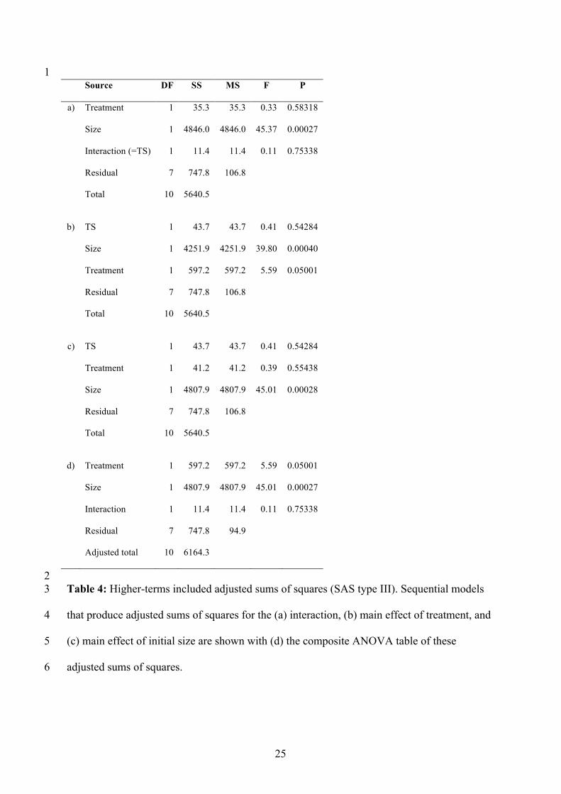
2 Table 4: Higher-terms included adjusted sums of squares (SAS type III). Sequential models 3

that produce adjusted sums of squares for the (a) interaction, (b) main effect of treatment, and 4

(c) main effect of initial size are shown with (d) the composite ANOVA table of these 5

adjusted sums of squares. 6

26

a) Collinear factors in ANOVA

Circles A and B represent the (approximately equal) sums of squares explained by the main effects of factors A and B (no interaction model).

Imbalance in the data introduces a positive correlation between A and B and results in shared, overlapping variation where the circles intersect.

b) Sequential model: A + B

When placed first in the sequence, factor A is attributed all of the overlapping variation.

c) Sequential model: B + A If the order is reversed, B (ignoring A) is attributed all of the shared variation and A (eliminating B) is reduced.

d) Full decomposition

Comparison of the two sequential models in b) and c) allows a full decomposition into the ‘unique’ effects of A and B plus the shared variation.

A B

A B

A B

A unique B unique

1

Figure 1 Venn diagram illustration of sums of squares partitioning for non-orthogonal factors 2 A and B (without interaction) using different sequential ANOVA models (a – d). Only the 3 sums of squares for the main effects of A and B are illustrated (the total and error sums of 4 squares are not shown). 5