confidence intervals for a variance ratio, or for ... · confidence intervals for a variance ratio,...

Confidence Intervals for a Variance Ratio, or for Heritability, in an Unbalanced Mixed LinearModelAuthor(s): David A. Harville and Alan P. FenechReviewed work(s):Source: Biometrics, Vol. 41, No. 1 (Mar., 1985), pp. 137-152Published by: International Biometric SocietyStable URL: http://www.jstor.org/stable/2530650 .Accessed: 31/05/2012 14:29

Your use of the JSTOR archive indicates your acceptance of the Terms & Conditions of Use, available at .http://www.jstor.org/page/info/about/policies/terms.jsp

JSTOR is a not-for-profit service that helps scholars, researchers, and students discover, use, and build upon a wide range ofcontent in a trusted digital archive. We use information technology and tools to increase productivity and facilitate new formsof scholarship. For more information about JSTOR, please contact [email protected].

International Biometric Society is collaborating with JSTOR to digitize, preserve and extend access toBiometrics.

http://www.jstor.org

http://www.jstor.org/action/showPublisher?publisherCode=ibs

http://www.jstor.org/stable/2530650?origin=JSTOR-pdf

http://www.jstor.org/page/info/about/policies/terms.jsp

BIOMETRICS 41, 137-152 March 1985

Confidence Intervals for a Variance Ratio, or for Heritability, in an Unbalanced Mixed Linear Model

David A. Harville Department of Statistics, Iowa State University, Ames, Iowa 50011, U.S.A.

and Alan P. Fenech

Division of Statistics, University of California, Davis, California 95616, U.S.A.

SUMMARY

A procedure is presented for constructing an exact confidence interval for the ratio of the two variance components in a possibly unbalanced mixed linear model that contains a single set of m random effects. This procedure can be used in animal and plant breeding problems to obtain an exact confidence interval for a heritability. The confidence interval can be defined in terms of the output of a least squares analysis. It can be computed by a graphical or iterative technique requiring the diagonalization of an m x m matrix or, alternatively, the inversion of a number of m x m matrices. Confidence intervals that are approximate can be obtained with much less computational burden, using either of two approaches. The various confidence interval procedures can be extended to some problems in which the mixed linear model contains more than one set of random effects. Correspond- ing to each interval procedure is a significance test and one or more estimators.

1. Introduction

Mixed and random linear models for classificatory data structures contain one or more sets of random main or interaction effects. Each of these sets, along with the set of residual effects, is assumed to have a different common variance, known as a variance component. These models have important biological and agricultural applications. One objective may be inference about the ratio of the variance of a particular set of random effects to the variance of the residual effects. In particular, animal and plant breeders often investigate the heritability of some trait, and, under certain assumptions, heritability is expressible as a strictly increasing function of a variance-component ratio. Commonly, the data are unbalanced.

Many methods are available for the point estimation of variance components and variance-component ratios, and these methods and their application have been extensively discussed (e.g., Searle, 1971; Harville, 1977; Thompson, 1979). For balanced data, confidence interval procedures are readily available (e.g., Graybill, 1976, Chap. 15). However, for unbalanced data, the literature on confidence intervals tends to focus on special cases or to invoke unrealistic assumptions (Wald, 1940, 1947; Spj0tvoll, 1968; Thomsen, 1975) or is not altogether instructive about various computational aspects (Thompson, 1955; Hartley and Rao, 1967; Seely and El-Bassiouni, 1983).

Here, we present some procedures for constructing exact or approximate confidence intervals for the variance ratio in any mixed linear model containing a single set of random effects (??3 and 5). The results are illustrated in the context of a specific animal breeding

Key words: Confidence intervals; Heritability; Mixed linear models; Unbalanced data; Variance components.

137

138 Biometrics, March 1985

application. Computational aspects are considered in ?4. Corresponding to each confidence interval procedure, there is a different estimation and testing procedure, as discussed and illustrated in ??6 and 7. In the final section, we consider extensions to the case of heteroscedastic or correlated random effects and to mixed and random models containing more than one set of random effects.

2. Preliminaries

2.1 General Formulation of the Problem

Let y represent an n x 1 observable random vector. Consider the mixed linear model

y = Xft + Zs + e, (2.1)

where , is a p x 1 vector of unknown parameters and where s and e are unobservable random vectors of dimensions m x 1 and n x 1 that are distributed independently as MVN(O, ar2I) (multivariate normal with mean vector 0 and variance-covariance matrix oK2I) and MVN(O, oK1I), respectively. Thus, the elements of s consist of a single set of "random effects," while the elements of e are random "errors."

The quantities X and Z are given matrices. Define r = rank(X, Z) - rank(X), p* -

rank(X), and f = n - rank(X, Z). It is assumed that r > 0 andf > 0. Let y = a 2/U2 represent the variance ratio. Then, var(y) = o2I + r2ZZ' = U2V, with

V = I + yZZ'. The variance components a 2 and a 2 are taken to be unknown parameters satisfying a2 2 0 and a2 > 0. Consequently, y >- 0. Note, however, that V is positive definite for all -y in the interval - 1/X* < -y < oo, where X* is the largest characteristic value of ZZ' (or, equivalently, of Z'Z). Thus, a model for y that is slightly more general than mixed model (2.1) can be obtained by specifying only that y - MVN[X,6, ao2(I + yZZ')] and by simply regarding -y as a parameter belonging to the interval Y > -1 /X*.

In what follows, we consider inference about -y and about strictly increasing (or decreasing) functions of -y (both under the constraint -y - 0 and under the weaker constraint y > -1 /X*). In particular, we consider the construction of confidence intervals for 'Y.

2.2 Lamb- Weight Data

For purposes of illustration, we introduce in Table 1 some data consisting of the weights at birth of 62 single-birth male lambs. These data (provided by G. E. Bradford, Department of Animal Science, University of California, Davis) come from five distinct population lines (two control lines and three selection lines). Each lamb was the progeny of one of 23 rams, and each lamb had a different dam. Age of dam was recorded as belonging to one of three categories, numbered 1 (1-2 years), 2 (2-3 years), and 3 (over 3 years).

Let Yijkd represent the dth of those lambs that are the offspring of the kth sire in the jth population line and of a dam belonging to the ith age category. A possible model for Yijkd is the mixed linear model

Yijkd = I + 3i + ir, + Sjk + eiJkd,

where the age effects ((1, 62, 63) and the line effects (7r, . . ., i5) are fixed effects, the sire (within line) effects (sl1, Sl2, . . ., S58) are random effects that are distributed independently as N(O, a 2), and the random errors elII1, ell2l,..., e3582 are distributed as N(0, aJe)

independently of each other and of the sire effects. Clearly, this model is expressible as a special case of mixed linear model (2.1).

Define the parametric function h2 = 4 U2/(U2 + o-2), which is interpretable as a heritability. We have that h2 = 4y/(l + -y) and, for -y > 0, h2 = 4/(1 + -y') and, conversely, that y =

Confidence Intervals for a Variance Ratio 139

Table 1 Birth weights (in pounds) of lambs

Dam Dam Dam Sire age Weight Sire age Weight Sire age Weight

Line 1 Line 3 Line 5

1 1 6.2 1 2 9.0 1 1 11.7 2 1 13.0 3 9.5 12.6 3 1 9.5 12.6 2 1 9.0

10.1 2 1 11.0 3 11.0 11.4 2 10.1 3 3 9.0

2 11.8 11.7 12.0 3 12.9 3 8.5 4 3 9.9

13.1 8.8 5 2 13.5 4 1 10.4 9.9 6 2 10.9

2 8.5 10.9 3 5.9 11.0 7 2 10.0

Line 2 13.9 12.7 3 1 11.6 3 13.2

1 3 13.5 3 13.0 13.3 2 2 10.1 4 2 12.0 8 1 10.7

3 11.0 11.0 14.0 Line 4 12.5 15.5 3 9.0

3 1 12.0 1 1 9.2 10.2 4 1 11.5 10.6

3 10.8 10.6 3 7.7

10.0 11.2

2 1 10.2 10.9

3 1 11.7 3 9.9

h2A4 - h2). Clearly, h2 is a strictly increasing function of y over the domain 0 < -y < 0o, with h2 = 0 when -y = 0 and with h2-- 4 when y --> oo. Since a heritability is inherently less than or equal to 1, there is an implicit assumption that 0 < h 1 I or, in terms of a, that 0 < Y . 3.

2.3 An Analysis of Variance (ANO VA) A significance test of the null hypothesis that y = 0 (or, equivalently, that a 2 = 0 or that h2 = 0) can be obtained from the following ANOVA table:

Source df SS MS EMS F p*= 7 So = 7454.959

after r= 18 Ss = 80.296 4.460 i2 + K.72 = i2 + 2.2118 f.2 F= 1.615 Error f= 37 Se = 102.235 2.763 i'e

Here, S# = y'Pxy, Ss = s'q, Se = y'y - S- S, and K = (I/r)tr(C), where Px = X(X'X)-X' [(X'X)- is an arbitrary generalized inverse of X'X], C = Z' (I - Px)Z, q = Z' (I - Px)y, and where s is any solution to the linear system

CsC= q (2.2)


or, equivalently, ft and s are the components of any solution to the linear system

E x'x x'Z][s] [Z'y](2.3) _Z'X Z1Z 'LJLJLL'Y

Equations (2.3) are normal equations (NE) obtained by treating s, like f, as a vector of unknown parameters and applying ordinary least squares. Equations (2.2) are obtained from NE (2.3) by absorbing the equations for , into those for s (Searle, 1971, ??7.1 and 10.9) and are called the reduced NE. It is known, and can be confirmed by applying standard results on the distribution

of quadratic forms, that S, and Se are distributed independently and that Se/ge x2(f) (a chi-square distribution with f degrees of freedom). Further, if the null hypothesis is true, then SI/(o + KoU2) _ X2(r). [If the null hypothesis is false, then the distribution of Ss/(a2 + K U2) is not, in general, X2(r), but rather is that of a nontrivial linear combination of two or more independently distributed chi-square random variables.] Thus, under the null hypothesis, the distribution of F is F(r, f) (an F distribution with r and f degrees of freedom), so that a significance test of the null hypothesis is obtained by finding the value of a (called the P-value) for which the observed value of F equals F* [the upper a point of the F(r, f) distribution]. The P-value for the lamb-weight data is .11.

The traditional method for the point estimation of a 2 and a(2, which is known as the fitting-constants method or Henderson's Method 3 (Searle, 1971, ?10.4), is also based on the ANOVA table. For the lamb-weight data, the estimates are

e= 2.763 and J2 = (4.460 - 2.763)/2.2118 = 0.767.

We can, by substitution, convert these estimates into estimates of y and h2, obtaining = e= 0.278 and 2 = 4/(1 + e-) = 0.87.

3. Exact Confidence Intervals

Let a represent an arbitrary real number (0 < a < 1). We shall derive a 100(1 - a)% confidence interval for y. To do so, we shall require some results on matrices and on linear models.

It is known that rank(C) = r (e.g., Marsaglia and Styan, 1974, p. 441). Let Al..., Ar represent the nonzero (and hence positive) characteristic values of C, and let D = diag(A 1 . . . a r) Take R and U to be matrices of dimensions m x r and m x (m - r) whose columns are orthonormal characteristic vectors of C corresponding to the values /\1,..., Z\r, 0,..., 0, respectively. That is, R is an m X r matrix such that R'R = I and CR = RD, and U is an m X (m - r) matrix such that U'U = I and CU = 0 (and R' U = 0). Then, P = (R, U) is an orthogonal matrix, and

R'CR = D, C = (PP')C(PP') = (RR' + UU')C(RR' + UU') = RDR', (3.1)

C2R = C(CR) = CRD = RD2, R'C2R = D2. (3.2)

Also, using C+ to represent the Moore-Penrose inverse of C, we note that

C+ = RD-1R'. (3.3)

If s, like fl, were treated as a vector of unknown parameters, then (i) a necessary and sufficient condition for a linear function X's to be estimable would be the existence of a vector I such that X' = I' C and (ii) there would exist an r X 1 vector of linearly independent estimable functions of s (e.g., Thompson, 1955, ?2.3). In fact, one such vector is the vector

t = (tj, ..., tr)' = D1/2R's = D-1/2(RD)'s = D-1/2R'Cs.


Let

t =" Wt,*** r'=D RS- = D- /RfCS = D- /Rfq 34

so that, if s were a vector of unknown parameters, t1,..., tr would be the best unbiased estimators of t1, . . ., tr, respectively.

Using the properties PxX = X, Px =P = P2 (e.g., Searle, 1971, ?1.5), we deduce that the distribution of q is multivariate normal with

E(q) = 0, var(q) = a2Z'(I - PX)V(I - Px)Z = o2(C + yC2).

Hence, the distribution of t is multivariate normal with

E(t) = 0, (3.5)

var(t) = 2D-1/2R'(C + yC2)RD-1/2 = o2(I + yD) (3.6)

= Cediag(1 + -y j, 1 + -YAr).

Note that the diagonal matrix I + yD is positive definite if and only if Y > -1 /A* (and nonnegative definite if and only if -y 2 -1/A*), where A* = max(A1,.. ., Ar). Note also that-~1/z\* < -1/X* (since, for y> >1/X* and Se - 1, I + yD is a variance-covariance matrix and thus is nonnegative definite), so that in general there exist values of -Y (namely, those in the interval - 1/A* < -y < - 1/X*) for which I + yD is positive definite but V is not positive definite or even positive semidefinite.

For -1/ /* < -y < oo, define

G(y; ) = (/r)t(I + yD)t (f) E i/( (.7) (1/f )Se kri SeA

By using standard results on the distribution of linear and quadratic forms (e.g., Searle, 1971, ?2.5), we can show (for -1/X* < y < o0) that

t'(I + yD)- t/e = t'[var(t)]- t - x2(r)

and that Se is distributed independently of q and hence of t and oft '(I + yD)-' t. Recalling that Se/IC x2(f), we conclude that (for -1/X* < -y < o0) G(y; y) - F(r, f). Since the distribution of G(-y; y) does not depend on any unknown parameters, G(-y; y) can serve as a "pivotal quantity" for constructing a confidence set for y (Cox and Hinkley, 1974, p. 21 1).

As a function of ay, G(-y; y) is strictly decreasing and (as can be confirmed, for example, by examining its second derivative) strictly convex. Further,

limit G(-y; y) = o0, limit G(-y; y) = 0,

and since

E t2 = t't = g'RDR'g= -'0 = g'q= S,, (3.8)

we have

G(0; y) = e = F.

For convenience, define G(-1/A/*; y) = o0 and G(oo; y) = 0. For the lamb-weight data, A ..., Ar and the corresponding observed values of t1,....


tr were as shown in the following table:

A t A t At 0.8400 -2.9062 1.4078 1.2882 2.7482 -2.5893 0.9027 -0.4508 1.7077 -2.5007 3.1505 -2.4773 1.0000 -4.8083 1.9329 -2.1365 3.3236 3.0048 1.0750 0.7319 2.0000 -1.5313 3.5644 -1.5521 1.1644 -0.7361 2.0000 0.9594 4.2340 -1.8835 1.3456 1.2924 2.3293 -1.2735 5.0875 0.7676

Thus, -1//* = -0.197, while -1/X* = -0.111. The function G(-y; y) is plotted in Figure 1.

Define a, and a2 to be arbitrary nonnegative real numbers such that a] + a2 = a. Define y I(y) and Y2(Y) by

G(yI(y); y) = F*, G (2(y); y) = F*Ca2. (3.9)

Since G(-y; y) is a strictly decreasing function of y and since G(,y; y) - F(r, f),

Pr[YI(y) < -Y 72 (Y)] = Pr[FI'a2 S G(y; y) Fa*] = 1 - a2- a, = 1 -a.

2.5

G

_2n11~~~~~ -*-*-- Gi 2.0 -@--e

1.640

1.0

0.568 \ N

-1 -0.008 1.125 2 3 4 5

Figure 1. Plots of the "pivotal quantities" for constructing exact or approximate confidence intervals for the variance ratio -y.


We conclude that

al I(Y) 6< 'Y 6 82(Y) (3.10) is a 100(1 - a)% confidence interval for y.

Consider again the lamb-weight example. Suppose that a, = a2 = .10, in which case F= 1.640 and F1*2 = 0.568. Then, referring to Figure -1, we see that ay(Y) = -0.008 and 'Y2(Y) = 1.125, i.e., an 80% confidence interval for y is -0.008 6 zy 6 1.125.

As is evident from the example, the lower bound ayI (y) may be negative, in which case the confidence interval contains negative values and hence values outside the parameter space 0 6 y < oo. [The bound yi(Y) may likewise violate the weaker constraint -1/X* < y.] It is also possible for A2(Y) to be negative, in which case the entire confidence interval consists of negative values. However, even in instances where part or all of the confidence interval lies outside the parameter space, the interval (in particular, its width and the extent of its inconsistency with the parameter space) may still be of interest (Cox and Hinkley, 1974, Chap. 7).

If we wish, we can modify the confidence interval to exclude negative values. Define 7y1(y) = max[0, yi(Y)] and ayt(y) = max[0, 'Y2(Y)]. Consider the interval y1*(y) 6 ' ly t(y). As can be easily verified, its probability of coverage equals 1 - a if 'y > 0, and equals 1 - a1 if y = 0. If there is an implicit upper bound on the parameter Y [e.g., 3 when 4/(1 + ay -) is interpretable as a heritability], the confidence interval can be further modified by changing either endpoint to I whenever that endpoint exceeds 1

A confidence interval for y can be readily converted into a confidence interval for any strictly increasing (or decreasing) function of y. In particular, a 100(1 - a)% confidence interval for h2 = 4,y/(l + y) is hi'(y) 6 zy ht(y), where hi'(y) = 4,y1(y)/[1 + ayl(y)] and ht(y) = 4'yt(y)/[1 + ayt(y)]. For the example, the 80% confidence interval 0 zy 6 1.125 converts into the interval 0 < h 2 2.12, which covers the entire parameter space. Thus, the data in the example, considered alone, do not seem to provide much information about the value of h2. This imprecision is not surprising, since not only are these data quite limited in extent, but they are also extremely unbalanced.

In the construction of the 100(1 - a)% confidence interval, the relative values assigned to a, and a2 should reflect the objectives of the investigation. If we take a I = 0 and a2 =

a, the 100(1 - a)% confidence interval becomes -1/A* < Y 6 a(Y), so that in effect we produce an upper (confidence) bound for y. If, at the other extreme, we take a, = a and a2 = 0, the interval becomes ay I(Y) < y < oo, and the entire emphasis is on obtaining a "tight" lower bound for y.

The approach we have taken in arriving at exact confidence intervals for y is similar to that of Thompson (1955) and to that taken in special cases by, e.g., Wald (1940), Spj0tvoll (1968), and Thomsen (1975). It can be verified that this approach is equivalent to the general approach outlined by Seely and El-Bassiouni (1983, ?2) and also to the seemingly different approach proposed by Hartley and Rao (1967, ?9).

4. Computational Considerations

To construct the exact 100(1 - a)% confidence interval for y, we must find the solution to each of the two nonlinear equations (3.9) [in ayl (y) and Y2(Y), respectively]. One approach is the graphical approach illustrated in ?3, which consists of plotting the function G(y; y) for -1 /A* < y < oo and "reading off" the values of y at which G(y; y) attains the values F* and F*L<2. An alternative approach is to employ some general iterative method for solving a nonlinear equation (e.g., Newton's method).

In applying an iterative method, we would, as in plotting G(y; y), have to evaluate the function G y; y) for each of a number of - values. In fact, some iterative methods may


also call for the evaluation of the first and possibly second derivatives of G(y; y). We find that

dy; Y)( f)S lI + iYA)2' (4.1)

d (2; - =2r e (1 + -A )3I (4.2)

With the graphical approach, intervals for additional values of a (or a, and a2) can be constructed with essentially no additional computations. On the other hand, the iterative approach offers greater numerical precision with (at least in the case of a single confidence interval) fewer function evaluations.

We now outline a computational procedure, which can be used in conjunction with either the graphical or iterative approach, to carry out the necessary function evaluations. The procedure operates on the elements of the symmetric array

Z'X Z'Z Z'Y

and consists essentially of the following five steps: (i) Compute a solution to the linear system X ' X(H, a) = (X 'Z, X ' y), e.g., by computing

a generalized inverse (X' X)- and forming the matrix H = (X' X)-X' Z and the vector a = (X'X)X'y.

(ii) Compute C = (Z'Z) - (Z'X)H and q = (Z'y) - (Z'X)a. (iii) Compute the characteristic values Al,..., Ar and the columns of RD112, i.e.,

corresponding orthogonal characteristic vectors of lengths 1/(A1 )1/2 1Alr) /2, respectively.

(iv) Compute t and Se from t = (RD 12)'q and Se = y'y - a'X'y - i tZ . [The formula for Se is a consequence of result (3.8).]

(v) Use formulas (3.7), (4.1), and (4.2) to compute, as required, the values of G(y; y) (and perhaps those of its first and second derivatives) corresponding to various values of 'Y.

The primary difficulty with this procedure is the burden imposed by the computation of the characteristic values and vectors. We now investigate the extent to which this difficulty can be circumvented. Consider, for -1 /A* < y < oo, the linear system

(I + YC)u = q (4.3) in u. It is shown in the Appendix that (for - 1/A* < y < oo) the matrix I + yC is positive definite and hence nonsingular, implying that linear system (4.3) is consistent and in fact has a unique solution. Subsequently, we use u to represent the solution to linear system (4.3), i.e., we take u = (I + ayC)-q. Note that u is functionally dependent on 'Y.

Results (A.5)-(A.8) from the Appendix can be used to reexpress G(y; y) and its first and second derivatives as

G((y; y) Su (4) Se u'(C + eI)u, (4.4)

dG (; y) _ 2 dG(; y) 2 u'(I + yCY1Cu. (4.5)

By using these expressions, rather than expressions (3.7), (4.1), and (4.2), we could evaluate


G(y; y) and its first and second derivatives without having to compute characteristic values and vectors. Note, however, that to do so, we would have to invert a different m x m matrix for each value of y. Consequently, this modification would be advantageous only if the evaluation of G(y; y) could be limited to a sufficiently small number of 'y values.

In applications where Z'Z is diagonal (or, more generally, where Z'Z and I + 'yZ'Z are easy to "invert") and p is small relative to m (as in the lamb-weight example or in any one-way random model), the computations expended in solving linear systems (2.2) and (4.3) can be greatly reduced. This reduction can be achieved, e.g., by recognizing that the matrix

(Z'Z) + (Z'Z)Z'X[X'X - X'Z(Z'Z)-Z'XLX'Z(Z'Z)

is a generalized inverse of C and by making use of the formula

(I + yC) 1 = (I + 'yZ'Z)- + 'y(I + yZ'Z)-1Z'X[X'X - yX'Z(I + yZ'Z)-1Z'X]-X'Z(I + yZ'Z)-"

(Henderson and Searle, 1981, ?4). As discussed, e.g., by Harville (1977, ?3), the linear system (4.3) is equivalent to the

linear system

[IX zX'Z [V4,Y (4.6)

in the sense that the lower m x 1 subvector of any solution to linear system (4.6) equals u and the lower right m x m submatrix of any generalized inverse of the coefficient matrix of linear system (4.6) equals (I + yC)-'. Thus, our discussion of the use of formulas (4.4) and (4.5) could be recast in terms of linear system (4.6). If linear system (4.6) is reexpressed as a linear system in ,B and ayui (which can be done for y $ 0), it is identical to Henderson's (1963) mixed-model equations.

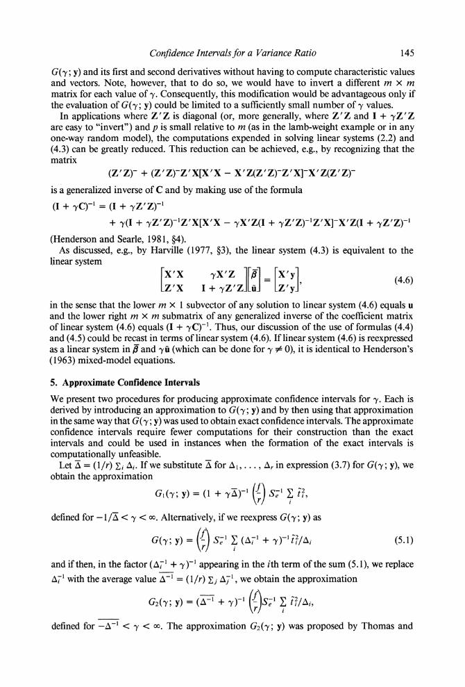
5. Approximate Confidence Intervals

We present two procedures for producing approximate confidence intervals for y. Each is derived by introducing an approximation to G(y; y) and by then using that approximation in the same way that G(y; y) was used to obtain exact confidence intervals. The approximate confidence intervals require fewer computations for their construction than the exact intervals and could be used in instances when the formation of the exact intervals is computationally unfeasible.

Let Ai = (1/r) Zi Ai. If we substitute Ai for I, . . ., Ar in expression (3.7) for G(y; y), we obtain the approximation

Gi~y; y) = (1 + yA)1 (j') Se I 9

defined for -1/A < y < o0. Alternatively, if we reexpress G(y; y) as

G(y; y) = (I') Se - (Ai- + 'y ti/iAj (5.1)

and if then, in the factor (A-1 + y)-1 appearing in the ith term of the sum (5.1), we replace -` with the average value A` = (1/r) Zj A', we obtain the approximation

G2(Y; y) =(A -+Y)l(f)S- te i7/A1,

defined for _lv-A <-y < o. The approximation G2(z; y) was proposed by Thomas and


Hultquist (1978) in the special case of the one-way random model. Observing that tr(C) = Zi Ai, and hence that A = K, and also that tr(C+) = Zi AT', we note that, by using results (3.8) and (A.9), the two approximations can be reexpressed as

GI(,y; y) = (1 + yA)-1G(O; y) = (1 + YK) 1F,

G2(Y; y) = [tr(C+) + ry]-f(f/Se)s'C+q.

Clearly, GI (O; y) = G(O; y), and, when y = 0, the distribution of GI (,y; y) is F(r, f). For ,y $ 0, the distribution of GI (,y; y) is F(r, f) if and only if AI = = Ar (as with balanced data). Further (for any value of y), the distribution of G2(y; y) is F(r, f) if and only if Al = *.* = Ar. In fact, ifA= =Ar, then GI(y;y) = G2(Y;y) = G(,y;y).

We have that

limit G2 (Y; Y) - 1. -Y_-,0 G(,y; y)

Thus, we can expect G2(Y; y) to approximate G(y; y) well for large values of ay, while, for small values of y, GI ('y; y) may provide a superior approximation. It is easy to show that the approximations GI ('y; y) and G2(Y; y), like G(y; y) itself, are strictly decreasing, strictly convex functions of y. Figure 1 includes plots of GI (,y; y) and G2(y; y) for the lamb-weight data.

The approximations G(zy; y) and G2(Y; y) produce the approximate 100(1 - a)% confidence intervals

(F - F*)/(KF*) y 6 (F - FI_2)/(KF L_2) (5.2)

and

(f/Se)g'C q - F*tr(C ) (f/Se)g'C q - F* .2tr(C+) aF

l rFIL 2 ,(5.3)

respectively. When applied to the lamb-weight data (with a I = a2 = .10), these intervals become the approximate 80% confidence intervals -0.007 < zy 6 0.833 and 0.063 6 y 6 1.310, respectively.

The computations required to form either of the approximate confidence intervals (5.2) and (5.3) are essentially those associated with the solution of a linear system of m equations in m unknowns, namely, linear system (2.2). In the case of interval (5.2), it suffices to solve linear system (2.2) by computing any generalized inverse C-, while in the case of interval (5.3), there is a specific requirement for the Moore-Penrose inverse C+. [The computation of the Moore-Penrose inverse is discussed, e.g., by Albert (1972, Chap. 5).] While, in general, the computations required to form interval (5.3) are more extensive than those required to form interval (5.2), the computations required to form either of these approximate intervals can be substantially fewer than the computations required to form the exact interval (3.10).

In an application where the computation of the exact interval (3.10) is unfeasible, approximate interval (5.2) could be used if ' is small, while approximate interval (5.3) could be employed if j is large [and if the computation of interval (5.3) is feasible].

6. Significance Tests

The procedures discussed in ??3 and 5 for constructing exact or approximate confidence intervals can be transformed, in the usual way, into procedures for performing exact or approximate significance tests. Suppose, for instance, that the null hypothesis is HO: z = 'Yo and the alternative hypothesis is HA: y > Hyo, where yo is a specified number belonging to the interval -1l/X* < Tyo < oo. Then, an exact significance test of Ho versus HA can be


obtained by locating the value of a for which G(yo; y) = F*. (This value is the P-value of the test.) Or, equivalently, we can set a I = a and a2 = 0 in the exact confidence interval procedure and locate the value of a for which the 100(1 - a)% lower confidence bound ,yi(y) equals yo. To obtain an approximate significance test, it suffices to find the a value for which GI ('yo; y) or G2Q(0; y) equals F*. These exact or approximate tests can equally well be regarded as tests of the null hypothesis y < yo versus the alternative hypothesis -y > Yo.

In the special case yo = 0, the null and alternative hypotheses y = 'Yo and 'y > 'Yo are equivalent to the hypotheses a = 0 and a 2 > 0, respectively. Moreover, G(0; y) = GI (0; y) = F, so that, in this special case, the exact significance test and the test based on GI ('Yo; y) both reduce to the ordinary F test.

An exact or approximate significance test of the null hypothesis 'y = 'Yo (or y >, 'yo) versus the alternative hypothesis y < yo can be obtained via an analogous approach. In particular, an exact test can be obtained by locating the a value for which G(yo; y) equals F 'o. The various null and alternative hypotheses about y can, of course, be reexpressed in terms of h2, and the significance tests reinterpreted accordingly.

7. Estimators

The pivotal quantity G(,y; y) and the two approximations Gl(,y; y) and G2('y; y) can be used to produce point estimators, as well as confidence intervals and significance tests. Point estimators A, a, and i2 of y are obtained by equating G(y; y), Gl(,y; y), and G2(y; y), respectively, to an appropriately chosen constant c and by then solving for the value of y. Thus, by definition,

G( A; y) = c, GI(Al; y) = c, G2(A2; y) = c. (7.1)

Note that the equation G(A; y) = c in A is of the same general form as equations (3.9), which must be solved to implement the exact confidence interval procedure. Thus, to compute y, we can apply the same graphical or iterative procedure used to compute the endpoints ayI (y) and 72(Y) of the exact confidence interval. The other two equations, G1(Al; y) = c and G2(A 2; y) = c, have explicit solutions

F - c (f/Se)s'C'q - c tr(C+) I = c Y2- rc

so that AI

and A2 can (in general) be computed more easily than Aj We discuss three alternative choices for c: c = 1, c = f/(f - 2), and c = F.50. Clearly,

f/(f- 2) > 1 and, according to Groeneveld and Meeden (1 977), f/(f- 2) > F*0. Further, F.50 = 1 for r =f and it appears that F 50 > 1 for r > fand that F 50 < 1 for r <f Note that each of the estimates 'y, 'l 1, and 'j2 is a strictly decreasing function of c.

The choice c = 1 is of interest because, when c = 1, ay equals j, i.e., 'y is identical to the estimator obtained via Henderson's Method 3.

Consider now the choice c = f/(f- 2). Observing that [since Se/e x2(f)] E(f/Se) = a2 )E[(SeI2)-l ] = ( 1/)f/(f- 2) and that

E[0/(1 + ayAi) =E[(1 + )1 =E[(&-' +y)-' P/,Aj =ra 2e

[as can be easily verified by, e.g., using results (3.5) and (3.6)] and recalling that Se is distributed independently of t and hence of any function of t, we find that

E[G(y; y)] = E[GI(,y; y)] = E[G2(Y; y)] = f/(f- 2). Thus, for the choice c = f/(f - 2), equations (7.1) are the equations obtained by equating


G(y; y), G('y; y), and G2(Y; y), respectively, to their expectations. Moreover, for this choice, 'I and ' are unbiased estimators of y, as can be easily verified. When c = f/(f - 2), the three equations (7.1) all satisfy Godambe's (1960) definition of an estimating equation and his criterion for assessing the efficiency of an estimating equation provides a possible basis for comparisons.

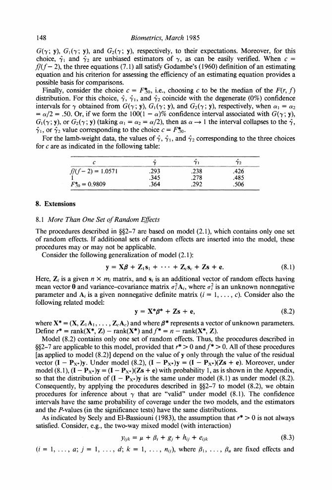
Finally, consider the choice c = F.50, i.e., choosing c to be the median of the F(r, f) distribution. For this choice, a, 'I, and '2 coincide with the degenerate (0%) confidence intervals for y obtained from G(y; y), G('y; y), and G2(Y; y), respectively, when a, = a2 = a/2 = .50. Or, if we form the 100(1 - a)% confidence interval associated with G(y; y), GQ(y; y), or G2(y; y) (taking a I = a2 = a/2), then as a -) 1 the interval collapses to the 'a, a , or 2 value corresponding to the choice c = F50.

For the lamb-weight data, the values of y, y 1, and 72 corresponding to the three choices for c are as indicated in the following table:

C y 'Y 72

f/(f - 2) = 1.0571 .293 .238 .426 1 .345 .278 .485 F*o= 0.9809 .364 .292 .506

8. Extensions

8.1 More Than One Set of Random Effects

The procedures described in ??2-7 are based on model (2.1), which contains only one set of random effects. If additional sets of random effects are inserted into the model, these procedures may or may not be applicable.

Consider the following generalization of model (2.1):

y = XB + Zis+ + +Zs+Zs + e. (8.1)

Here, Zi is a given n x mi matrix, and si is an additional vector of random effects having mean vector 0 and variance-covariance matrix aiAi, where aJ is an unknown nonnegative parameter and Ai is a given nonnegative definite matrix (i = 1, . . ., c). Consider also the following related model:

y= X*,B* + Zs + e, (8.2)

where X* = (X, ZIA1,,.. ., ZCAc) and where ,* represents a vector of unknown parameters. Define r* = rank(X*, Z) - rank(X*) andf* = n - rank(X*, Z).

Model (8.2) contains only one set of random effects. Thus, the procedures described in ??2-7 are applicable to this model, provided that r* > 0 andf* > 0. All of these procedures [as applied to model (8.2)] depend on the value of y only through the value of the residual vector (I - Px*)y. Under model (8.2), (I - Px*)y = (I - Px*)(Zs + e). Moreover, under model (8.1), (I - Px*)y = (I - Px*)(Zs + e) with probability 1, as is shown in the Appendix, so that the distribution of (I - Px*)y is the same under model (8.1) as under model (8.2). Consequently, by applying the procedures described in ??2-7 to model (8.2), we obtain procedures for inference about y that are "valid" under model (8.1). The confidence intervals have the same probability of coverage under the two models, and the estimators and the P-values (in the significance tests) have the same distributions.

As indicated by Seely and El-Bassiouni (1983), the assumption that r* > 0 is not always satisfied. Consider, e.g., the two-way mixed model (with interaction)

vijk = u + 3i + gj + hii + eijk (8.3)

(i =1, ..., a;j ==1,..., d;kk= =1, .,nij) ),wh hrefi, ...,laaareffixed effects and

Confidence Intervalsfor a Variance Ratio 149

where gl, ..., gd, hi,, h2l, .. ., had, elll, ..., eadna, are random effects and errors that are distributed independently as N(O, a2), N(0, (oh), and N(O, Us), respectively. Suppose (for simplicity,) that nij > 0 (i = I,... a; j = 1, ... ., d).

If we regard model (8.3) as a special case of model (8.1) with c = 1, 9 = ( fl, .. Y,

S1 = (gl, . . . gd)', Al =1, and s = (hi,, h2l, ..., had), wefindthatr* = ad-a-d+ 1 and that f* = n.. - ad. Thus, the procedures described in ??2-7 could be used to make inferences about the ratio a 2/Cr2 (provided that nij > 1 for some i and j). Suppose, however, that we wished to make inferences about the ratio a2a Regarding model (8.3) as a special case of model (8.1) with c = 1, A t = (, 3l,..., la)Y, SI = (hi,, h2l1,.. had)',

AI = I, and s = (g1,..., gd)', we find that r* = 0. We conclude that the procedures described in ??2-7 could not be used to make inferences about a /2ra.

We reach a different conclusion if we consider inferences about a 2/Cra under the alternative version of the two-way mixed model (e.g., Searle, 1971, ?9.7c) in which

cov(hij, hitj) = a 2 if i' = i and j' =j,

-~h/(a-1) if i'5i and j'=j,

=0 if j'$j.

Then Al = [a/(a - 1)]diag[I - (1/a)11'. .., I - (1/a)11 '], and it can be shown that r* - d - 1. Thus, under the alternative version of the two-way mixed model, the procedures described in ??2-7 could be used to make inferences about a 2/ca . The explanation for this seeming contradiction is that the variance component 2 has a different interpretation in one version of the model than in the other [as discussed, e.g., by Searle (1971)].

8.2 Correlated or Heteroscedastic Random Effects

Suppose that s MVN(O, a2A), where A is a given nonnegative definite matrix, rather than, as previously supposed, that s MVN(O, aH2I). Take Q to be an arbitrary nonsingular matrix such that Q'AQ = diag(I, 0), and let L = (Q')-'. Define partitionings Q -

(Qi, Q2) and L = (LI, L2), where the dimensions of both Qi and LI are m X rank(A). Note that A = L diag(I, O)L' = L 'L. Let Z* = ZL1 and s* = Q's.

We have that

Zs = Z(Q')-"Q's = Z(LIQ' + L2Q9)s = Z*s* + ZL2Q2s.

Further, E(Q's) = 0 and var(Q's) = 'Q2AQ2 = 0, so that Q's = 0 (with probability 1) and hence Z*s* = Zs (with probability 1). Thus, the distribution of y under the model y = Xft + Z*s* + e is the same as under the model y = Xft + Zs + e. Observing that s* is distributed as MVN(O, a 2I) independently of e, we see that, if we put Z* in place of Z, we can use the procedures described in ??2-7 to make inferences about the ratio a 2/Cr2.

In the lamb-weight example, the elements of s represent the sire (within line) effects. If some of the sires were inbred or were related to each other, it would not be altogether appropriate to take A = I. Rather, we should take A to be a certain positive definite matrix known as the numerator relationship matrix, in which case a particular choice for the matrix L can be computed from recursion formulas given by Henderson (1976). (Hender- son's approach requires that the vector s be expanded to include effects for all animals in the "base population.")

To make inferences about the ratio a 2/U2 in the alternative version of the two-way mixed model (8.3), we would set s = (h1I, h2h, . . . , had)', so that

A = [a/(a - )]diag[I - (1/a)11', ..., I - (1/a)11'].


Here, we could choose

Q. = [(a - l)/a]"/2diag(01, ... , Q), Q. = diag(l, ..., 1),

where 0 = [(I/a)"21, 0.] is an orthogonal matrix, e.g., a Helmert matrix (Searle, 1982, p. 71), in which case

L, = [a/(a - 1)]"/2diag(01,..., O.), L, = (l/a)diag(1,..., 1).

RfSUMf

On presente une construction d'un intervalle de confiance exacte du rapport de deux composantes de la variance sur un module lineaire mixte eventuellement desequilibre contenant un seul ensemble de m effets aleatoires. Cette procedure peut ere utilis&e dans des problemes de selection animale ou vegetale pour obtenir un intervalle de confiance exacte de l'heritabilite. L'intervalle de confiance peut ere defini en termes de sortie d'une analyse des moindres carries. I1 peut etre calcule par une technique graphique ou iterative demandant la diagonalisation d'une matrice d'ordre m, ou bien par inversion d'un certain nombre de matrices d'ordre mn. On peut obtenir des intervalles de confiance approches avec moins de calculs en utilisant ces deux voies. Ces difftrentes techniques de construction d'intervalles de confiance peuvent etre etendues a quelques problems dans lesquels le module lineaire mixte a plus d'un ensemble d'effets aleatoires. A chaque intervalle de confiance correspond un test d'hypothese et un ou plusieurs estimateurs.

REFERENCES

Albert, A. (1972). Regression and the Moore-Penrose Pseudoinverse. New York: Academic Press. Cox, D. R. and Hinkley, D. V. (1974). Theoretical Statistics. London: Chapman and Hall. Godambe, V. P. (1960). An optimum property of regular maximum likelihood estimation. Annals of

Mathematical Statistics 31, 1208-1211. Graybill, F. A. (1976). Theory and Application of the Linear Model. North Scituate, Massachusetts:

Duxbury. Groeneveld, R. A. and Meeden, G. (1977). The mode, median, and mean inequality. The American

Statistician 31, 120-12 1. Hartley, H. 0. and Rao, J. N. K. (1967). Maximum likelihood estimation for the mixed analysis of

variance model. Biometrika 54, 93-108. Harville, D. A. (1977). Maximum likelihood approaches to variance component estimation and to

related problems. Journal qf the American Statistical Association 72, 320-338. Henderson, C. R. (1963). Selection index and expected genetic advance. In Statistical Genetics and

Plant Breeding, W. D. Hanson and H. F. Robinson (eds), Publication 982, 141-163. Washington, D.C.: National Academy of Sciences, National Research Council.

Henderson, C. R. (1976). A simple method for computing the inverse of a numerator relationship matrix used in prediction of breeding values. Biometrics 32, 69-83.

Henderson, H. V. and Searle, S. R. (1981). On deriving the inverse of a sum of matrices. SIAM Review 23, 53-60.

Marsaglia, G. and Styan, G. P. H. (1974). Rank conditions for generalized inverses of partitioned matrices. Sankhya, Series A 36, 437-442.

Searle, S. R. (1971). Linear Models. New York: Wiley. Searle, S. R. (1982). Matrix Algebra Usefulfor Statistics. New York: Wiley. Seely, J. F. and El-Bassiouni, Y. (1983). Applying Wald's variance component test. Annals of Statistics

11, 197-201. Spj0tvoll, E. (1968). Confidence intervals and tests for variance ratios in unbalanced variance

components models. Review of the International Statistical Institute 36, 37-42. Thomas, J. D. and Hultquist, R. A. (1978). Interval estimation for the unbalanced case of the one-

way random effects model. Annals of Statistics 6, 582-587. Thompson, R. (1979). Sire evaluation. Biometrics 35, 339-353. Thompson, W. A., Jr. (1955). On the ratio of variances in the mixed incomplete block model. Annals

of Mathematical Statistics 26, 721-733. Thomsen, I. (1975). Testing hypotheses in unbalanced variance components models for two-way

layouts. Annals of Statistics 3, 257-265.


Wald, A. (1940). A note on the analysis of variance with unequal class frequencies. Annals of Mathematical Statistics 11, 96- 100.

Wald, A. (1947). A note on regression analysis. Annals of Mathematical Statistics 18, 586-589.

Received January 1984; revised July 1984.

APPENDIX

Some Properties of the Matrices I + -yC and C + -yC2 Observe that P'(I + -yC)P = diag(I + -yD, I), implying that I + -yC = P diag(I + 'yD, I)P'. Thus, I + -yC is positive definite if and only if I + -yD is positive definite, i.e., if and only if y > - 1/A*, in which case

(I + -yC)-' = P diag[(I + yD)-', I]P' = R(I + yD)-'R' + UU'. (A.1)

Making use of result (3.2), we find that

(C + yC2)P = P diag(D + ayD2, 0).

Thus, the columns of P form a set of orthonormal characteristic vectors of C + yC2, and the corresponding characteristic values of Al + ' A... ?r + '/r, 0,... 0. It follows that, for oy > -1 /A*, the Moore-Penrose inverse of C + yC2 is

(C + _yC2)+ = P diag[(D + ayD2)-', 0]P' = R(D + -yD2)-'R' = RD-I/2(I + -yD)-'D-/2R'. (A.2)

Further, observing that C + _yC2 = R(D + -yD2)R', we find that (for -y > -1/A*)

(C + _YC2)(C + _yC2)+ = RR' = I - UU',

(C + YC2)(C + YC2)+C = (I - UU')C = C,

(C + 'yC2)(C + yC2)+q = (C + YC2)(C + yC2)+Cj = Cj = q. (A.3)

Let w represent an arbitrary solution to the linear system

(C + YC2)w = q (ey > -1/A*)

[The consistency of this linear system follows from result (A.3).] Clearly, (I + yC)Cw = q, implying that Cw = (I + -yC)-'q = u and, in particular, that

C(C + yC2)+q = u (ey > 1/A*) (A.4)

Derivation of Alternative Expressions for the Pivotal Quantities and for Various Related Quantities

Making use of results (A.1), (A.2), (A.4), (3.1), (3.3), and (3.4), we find that, for y > -1/A*,

E I/(1 + -yzh) = t'(I + -yD)-'t = q'RD-"/2(I + yD)-'D-"/2R'q

= q'(C + _yC2)+q = q'(C + _YC2)+Cj = u's (A.5) = q'(C + YC2)+(C + YC2)(C + ryC2)+q = q'(C + YC2)+C(C- + yI)C(C + _yC2)+q

= u ' (C- + 'yI)u, (A.6)

E Ai2t/(l + yAi)2

= t'(I + -yD)-'D(I + -yD)-'t

q'[RD-/2(I + yD)-'D-/2R']RDR'RDR'[RD-"/2(I + D)-'D-/2R']q

= q ' (C + 'YC2)+C2 (C + 'yC2)+ q = W'u, (A.7)


E A t2/( 1 + -YZA)3

= t'(I + -yD)-'D'12(I + yD)-'D312(I + yD)-'t = q'[RD-"/2(I + yD)-'D-/2R']RDR'R(I + -yD)-'DR'R'[RW'1/2(I + yD)-'D-'1/2R']q

= q'(C + yC2)'CR(I + yD)-'DR'C(C + _YC2)+q = u'R(I + yD)-'DR'u = u'R(I + -yD)-'R'Cu = u'(I + yC)-'Cu, (A.8)

Pt2, = t g'fDt 1/2 D-D/2Rfq = s'RD-'R'q = s C+q, (A.9)

J (1 + -yzj) = det(I + -yD) = det(I + -yR'RD) = det(I + -yRDR') = det(I + yC), (A.10)

A zi/(I + -yAi) = tr[(I + yD)-'D] = tr[(I + yD)-'R'CR]

= tr[R(I + -yD)-'R'C] = tr[(I + yC)-'C], (A. 1)

z [z,/(l + yAz)]2 = tr[(I + yD)-'D(I + yD)-'D]

= tr[(I + yD)-1R'CR(I + yD)-1R'CR]

= tr[R(I + yD)-1R'CR(I + yD)-1R'C] = tr{[(I + _yC)-C]21. (A.12)

Distribution of (I - Px*)y Under Model (8. 1) Suppose that y follows model (8.1). Observe that (I - Px*)X* = 0 or, equivalently, that

(I-Px*)X = 0, (I-Px*)ZiAi = 0 (i= 1,..., c). We find that

(I - Px*)y = (I - Px*)Zisi + (I - Px*)(Zs + e).

Further, E[(I - Px*)Zisi] = 0 and

var[(I - Px*)Zisi] = cr(I - Px*)ZiAiZ'(I - Px*) = 0,

implying that (I - Px.)Zisi = 0 with probability 1 (i = 1,.. ., c). We conclude that (I - Px*)y = (I - Px*)(Zs + e) with probability 1.

confidence intervals for a variance ratio, or for ... · confidence intervals for a variance ratio,...

Documents