1 disjunctive model for the simultaneous optimization and...
TRANSCRIPT

Disjunctive Model for the Simultaneous Optimization and Heat Integration 1
with Unclassified Streams and Area Estimation 2
Natalia Quirantea, Ignacio E. Grossmannb, José A. Caballeroa,* 3
a Institute of Chemical Processes Engineering. University of Alicante, PO 99, E-03080 Alicante, Spain. 4
b Department of Chemical Engineering. Carnegie Mellon University, 5000 Forbes Ave., Pittsburgh, PA 5
15213, USA. 6
*Corresponding author: [email protected], Tel: +34 965902322. Fax: +34 965903826. 7
E-mail addresses: [email protected] (N. Quirante), [email protected] (I.E. Grossmann), 8
[email protected] (J.A. Caballero) 9
10
Abstract 11
In this paper, we propose a disjunctive formulation for the simultaneous chemical process 12
optimization and heat integration with unclassified process streams –streams that cannot be 13
classified a priori as hot or cold streams and whose final classification depend on the process 14
operating conditions–, variable inlet and outlet temperatures, variable flow rates, isothermal 15
process streams, and the possibility of using different utilities. The model is based on the original 16
formulation of the Pinch Location Method (PLM), but in this case, the ‘max’ operators are 17
represented by means of a disjunction. 18
The paper also presents an extension to allow area estimation assuming vertical heat transfer. The 19
model takes advantage of the disjunctive formulation of the ‘max’ operator to explicitly determine 20
all the ‘kink’ points on the hot and cold balanced composite curves and uses an implicit ordering 21
for determining adjacent points in the balanced composite curves for area estimation. 22
The numerical performance of the proposed approach is illustrated with four case studies. Results 23
show that the novel disjunctive model of the pinch location method has an excellent numerical 24
performance, even in large-scale models. 25
26
Keywords: simultaneous optimization, heat integration, variable temperatures, disjunctive 27
model, unclassified streams. 28
Nomenclature 29
30
1. Introduction 31
One of the greatest advances in chemical process engineering was the discovery by Hohmann 32
(1971) in his PhD thesis that it is possible to calculate the least amount of hot and cold utilities 33
required for a process without knowing the heat exchanger network. This advance motivated the 34
introduction of the pinch concept (Bodo Linnhoff & Flower, 1978a, 1978b; Umeda et al., 1978) 35
and the Pinch Design Method (B. Linnhoff & Hindmarsh, 1983), for the design of heat exchanger 36
networks (HEN). Since that, seminal works has been published thousands of papers related to 37
heat integration. 38
Without the intention of doing a comprehensive review, significant advances were developed in 39
the decades of 1980-90 of the last century. Papoulias and Grossmann (1983) presented a 40
mathematical programming that takes the form of a transshipment problem that allows calculating 41
the minimum utilities and the minimum number of matches (an alternative version that used a 42
transportation model was presented by Cerda et al. (1983). The first one to use the vertical heat 43
transfer concept that allows estimating the heat transfer area without knowing the explicit design 44
of a heat exchanger network was Jones in 1987 (Jones, 1987). The first automated HEN design, 45
relying on a sequential approach –minimum utilities calculation, followed by a minimum number 46
of heat exchangers and then the detailed network– was developed by Floudas et al. (1986). Later, 47
Ciric and Floudas (1991), Floudas and Ciric (1989, 1990), Yee and Grossmann (1990), and Yuan 48
et al. (1989) proposed different alternatives for the simultaneous design of the HEN, all of them 49
based on mathematical programming approaches. Comprehensive reviews of the advances in 50
HEN in the 20th century can be found in Gundersen and Naess (1988), Jezowski (1994a, 1994b), 51
and Furman and Sahinidis (2002). More recent reviews can be found in Morar and Agachi (2010) 52
and Klemeš and Kravanja (2013). 53
Pinch analysis has extended to almost all branches of chemical process engineering, for example, 54
Ahmetović presented a review of the literature for water and energy integration (Ahmetović et 55

al., 2015; Ahmetović & Kravanja, 2013). In El-Halwagi (2012) we can find the extension of the 56
pinch analysis to mass exchange networks and process integration. Tan and Foo (2007) extended 57
the pinch analysis to carbon-constrained energy sector planning. The cogeneration and total site 58
integration can be found in Raissi (1994) and Dhole and Linnhoff (1993). Wechsung et al. (2011) 59
and Onishi et al. (2014b) introduced the concept of work exchanger networks and the integration 60
of work and heat exchanger networks (WHEN). 61
One of the major limitations of the pinch technology applied to the design of heat exchanger 62
networks is that it had to be used once the chemical process has already been designed and all the 63
flows and temperatures fixed. However, the simultaneous design and optimization of the process 64
and the heat integration strategy could eventually produce larger benefits than a sequential 65
approach (Biegler et al. (1997) presented an illustrative example). 66
In a mathematical programming-based approach for the design of chemical processes, one 67
straightforward possibility to overcome this problem consists of extending the superstructure of 68
the process with that of the heat exchanger network. Nevertheless, the problem rapidly becomes 69
intractable due to the large number of variables (both continuous and integer) and equations. 70
Despite this problem, different researchers have solved relatively complex problems following 71
this approach (de la Cruz et al., 2014; Martelli et al.; Oliva et al., 2011; Onishi et al., 2014a; 72
Vázquez-Ojeda et al., 2013; Yee et al., 1990). To alleviate that problem, an alternative consists 73
of considering only the thermal effects (heat integration) without the design of a specific network; 74
in other words, including in the optimization only the utilities and their nature (e.g., low, medium 75
or high pressure steam) but not the investment costs in the heat exchangers network. The 76
underlying idea is that energy costs have much larger impact than investment costs and could 77
have an important effect when optimizing with the rest of the process. However, differences in 78
the investment of two heat exchanger networks with similar utilities and the same streams 79
involved are not expected to be significant at least when compares with the energy effects. 80
Under some conditions, it is possible to solve the Pinch Tableau problem at each iteration of the 81
optimization or explicitly include in the model the equations of the transshipment (or extended 82
transshipment) problem (Corbetta et al., 2016). For example, some of the superstructure-based 83

approaches for the design of chemical processes include those equations as a part of the model 84
(Ciric & Floudas, 1991). However, this approach relies on the concept of temperature interval. 85
While the temperature intervals are maintained in all the optimization, this is likely the best 86
alternative for dealing with the simultaneous optimization and heat integration problem, but if 87
inlet (outlet) temperatures can change, the number of temperature intervals and the streams 88
present in each interval change during the optimization. Mathematically this is equivalent to 89
introduce discontinuities and non-differentiabilities, and consequently, the complete optimization 90
can fail. 91
To overcome the previous problem Duran and Grossmann developed the Pinch Location Method 92
(PLM) (Duran & Grossmann, 1986). The idea was to develop a mathematical approach that does 93
not rely on the concept of temperature interval and, as a consequence, does not suffer from the 94
drawbacks of previous approaches. The major drawback of the original model presented by Duran 95
and Grossmann (1986) is that in their model appear the «max» operator. They proposed to use a 96
smooth approximation. However, the smooth approximation is non-convex and its numerical 97
behavior depends on parameters in the approximation function. 98
To avoid the non-differentiability introduced in the model of Duran and Grossmann (1986), 99
several approaches have employed binary variables to locate pinch temperatures. In fact, 100
Grossmann et al. (1998) presented a disjunctive formulation that explicitly takes into account the 101
location of a stream –above, across or below– potential pinch candidate. Navarro-Amorós et al. 102
(2013) presented an alternative MI(N)LP model that uses the concept of temperature intervals and 103
the transshipment problem for heat integration with variable temperatures. Quirante et al. (2017) 104
proposed a novel disjunctive model for the simultaneous optimization and heat integration of 105
systems with variable inlet and outlet temperatures, based on the formulation of the pinch location 106
method, modeling the ‘max’ operators by means of a disjunction. Kong et al. (2017) proposed an 107
extension of the Navarro-Amorós et al. (2013) model for the simultaneous chemical process 108
synthesis and heat integration considering also unclassified process streams. 109
A common situation that appears when the temperatures are not fixed is that a priori it is not 110
possible to decide if a process stream is a hot (it requires cooling) or a cold (it requires heating) 111

stream (Kong et al., 2017). The objective of this paper is to extend the research made in our last 112
work (Quirante et al., 2017) to the case in which there are unclassified process streams. The 113
proposed model has the advantage of reducing the number of equations and binary variables 114
compared to existing alternatives, which allows to reduce the CPU time when solving the 115
problems. 116
Besides, in a chemical process, usually more than a single hot and/or cold utility are present and 117
it is important to deal with the selection of the best set of utilities among all those available, and 118
some streams can suffer phase changes. In this paper, we will show how we can extend the pinch 119
location method to deal with all these cases. 120
A drawback of the PLM is that we ignore the contribution of the area to the total cost of the heat 121
exchanger network. Even though in most situations this is not a major problem because, as 122
commented above, the effect of the area can be ignored without affecting to the final solution, 123
this is not necessarily always the case. We will show that for problems of medium size it is 124
possible to simultaneously estimate the area of the HEN and consequently its investment cost. 125
The rest of the paper is structured as follows. In the two following sections, we present an 126
overview of the pinch location method. Then, we present the disjunctive model for solving 127
problems with unclassified streams and the extension to isothermal process streams and multiple 128
utilities. In section 4, we present how it is possible to include area estimation in the model using 129
the vertical heat transfer problem. In section 5, we present some case studies to illustrate the 130
performance of the proposed approach. Finally, we provide some conclusions obtained from this 131
work. 132
133
2. The Pinch Location Method. Overview 134
In a system in which all the heat flows are constant, the pinch point is always in the inlet 135
temperature of some of the process streams. Duran and Grossmann (1986) showed that for a fixed 136
minimum approach temperature (∆Tmin) between the hot and cold composite curves, if we 137
systematically calculate all the hot and cold utilities for all the pinch candidates (all the inlet 138

temperatures of the process streams), the correct answer corresponds to the candidate with the 139
largest heating and cooling utilities. Mathematically this result can be written as follows: 140
max ( ); max ( );p pH H C Cp STR p STR
Q Q Q Q
(1) 141
where STR is a set of all the process streams that are pinch candidates. QH, QC are the heating and 142
cooling utilities for a given ∆Tmin and ,p pH CQ Q are the heating and cooling utilities for each one of 143
the pinch candidates p. 144
In order to take into account that the hot and cold composite curves must be separated at least by 145
the minimum approach temperature, we must work with shifted temperatures. 146
Defining the following index sets: 147
HOT = [i | i is a hot stream] HOT STR
COLD = [j | j is a cold stream] COLD STR
The shifted temperatures can be defined as follows: 148
min
min
min
min
2
2
2
2
in ini i
out outi i
in inj j
out outj j
TTS Ti HOT
TTS T
Tts tj COLD
Tts t
∆ = − ∈∆ = −
∆ = + ∈∆ = +
(2) 149
where , , ,in out in outi i j jT T t t are the actual inlet and outlet stream process temperatures. 150
From a total heat balance, we obtain the following equation: 151
in out out inC H i i i j j j
i Hot j Cold
Q Q F T T f t t
(3) 152
where Fi is the heat capacity flowrate of the hot stream i and fj is the heat capacity flowrate of the 153
cold stream j. 154
Taking into account that the pinch point divides the problem into two heat balanced parts, to 155
calculate the hot utility requirements we need to study only the streams above the pinch and the 156
cold utilities can be calculated from the energy balance presented in Eq.(3) or vice versa, we can 157
calculate the cold utilities from the energy content of the streams below the pinch and the hot 158
utilities from the energy balance. 159
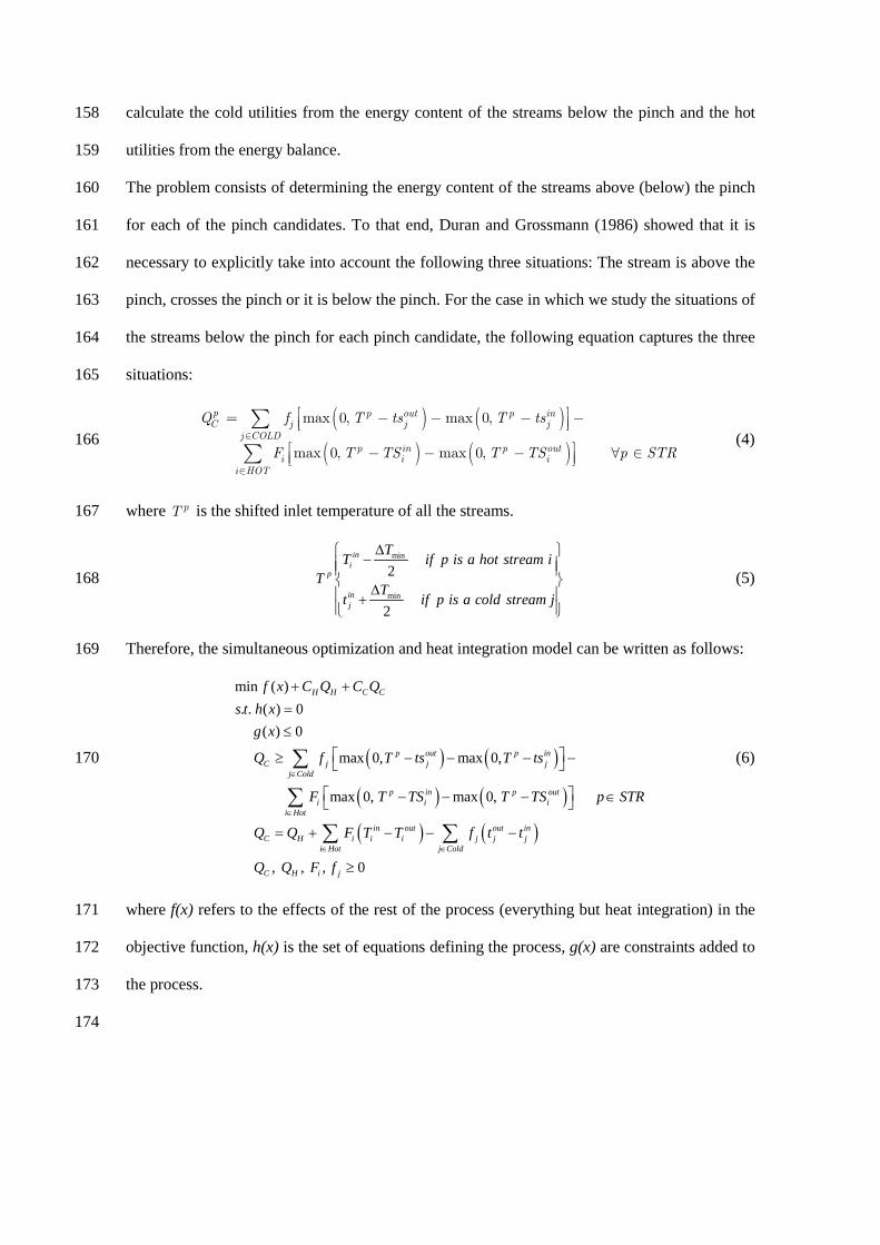
The problem consists of determining the energy content of the streams above (below) the pinch 160
for each of the pinch candidates. To that end, Duran and Grossmann (1986) showed that it is 161
necessary to explicitly take into account the following three situations: The stream is above the 162
pinch, crosses the pinch or it is below the pinch. For the case in which we study the situations of 163
the streams below the pinch for each pinch candidate, the following equation captures the three 164
situations: 165
max 0, max 0,
max 0, max 0,
p p out p inC j j j
j COLDp in p out
i i ii HOT
Q f T ts T ts
F T TS T TS p STR
(4) 166
where pT is the shifted inlet temperature of all the streams. 167
min
min
2
2
ini
p
inj
TT if p is a hot stream iT
Tt if p is a cold stream j
∆ − ∆ +
(5) 168
Therefore, the simultaneous optimization and heat integration model can be written as follows: 169
( ) ( )
( ) ( )( ) ( )
min ( ). . ( ) 0
( ) 0
max 0, max 0,
max 0, max 0,
,
H H C C
p out p inC j j j
j Cold
p in p outi i i
i Hot
in out out inC H i i i j j j
i Hot j Cold
C H
f x C Q C Qs t h x
g x
Q f T ts T ts
F T TS T TS p STR
Q Q F T T f t t
Q Q
∈
∈
∈ ∈
+ +=≤
≥ − − − −
− − − ∈
= + − − −
∑
∑
∑ ∑, , 0i jF f ≥
(6) 170
where f(x) refers to the effects of the rest of the process (everything but heat integration) in the 171
objective function, h(x) is the set of equations defining the process, g(x) are constraints added to 172
the process. 173
174

3. The Pinch Location Method with Unclassified Process Streams 175
In this section, we present a disjunctive model for the simultaneous optimization and heat 176
integration that also takes into account the possibility of including unclassified process streams. 177
These streams could behave as hot or cold streams depending on the operating conditions of the 178
rest of the process and, therefore, cannot be classified a priori. The model is based on the pinch 179
location in which the ‘max’ operators are replaced by disjunctions following the procedure 180
presented by Quirante et al. (2017). 181
To formally introduce the model let us define the following index sets: 182
STR = [s | s is a process stream] HOT = [i | i is a hot stream] HOT STR
COLD = [j | j is a cold stream] COLD STR
UNC = [k | k is an unclassified stream] UNC STR
Note that HOT COLD UNC STR 183
184
Classification constrains 185
Here we follow the approach presented by Kong et al. (2017). 186
s
0
0
in outs s s s
s
s
T T T T STR
T s HOT
T s COLD
+ −
−
+
− = − ∈
= ∀ ∈
= ∀ ∈
(7) 187
In Eq.(7), we have introduced the variables ,s sT T . The first one ( sT ) will take a positive value 188
for hot streams, and the second one ( sT ) for the cold streams. The correct classification of the 189
unclassified streams can be forced by the following disjunction: 190
0 0
0 0
k s
k k
k k
WH WC
T T k UNC
T T
+ −
− +
≥ ∨ ≥ ∀ ∈ = =
(8) 191
where WH and WC are Boolean variables that take the value of “True” if the stream ‘k’ is 192
classified as hot or cold respectively. This disjunction can be reformulated in terms of binary 193
variables using the hull reformulation (Trespalacios & Grossmann, 2014): 194

1
·
·
k k
k k k
k k k
wh wc
T T wh k UNC
T T wc
+ +
− −
+ = ≤ ∀ ∈
≤
(9) 195
where wh and wc are now binary variables that take the value 1 if the stream is classified as hot 196
or cold respectively, and 0 otherwise. 197
198
Definition of shifted temperatures 199
For the hot and cold streams, shifted temperatures are equivalent to those presented above Eq.(2) 200
(we rewrite them here for the sake of clarity): 201
min
min
min
min
2 i
2
2 j
2
in ini i
out outi i
in inj j
out outj j
TTS THOT
TTS T
TTS tCOLD
TTS t
∆ = − ∈∆ = −
∆ = + ∈∆ = +
(10) 202
The correct displacement of the unclassified streams can be forced with the following disjunction: 203
min min
min min
2 2
2 2
k k
in in in ink k k k
out out out outk k k k
WH WCT TTS T TS T k UNC
T TTS T TS T
∆ ∆ = − ∨ = + ∀ ∈ ∆ ∆ = − = +
(11) 204
The previous disjunction can be written in terms of binary variables using the hull reformulation 205
as follows: 206
, , , ,
, , , ,
min, , , ,
1
2
k kin in in out out outk H k C k k H k C k
in in in out out outk H k C k k H k C k
in in out ouH k H k k H k H k
wh wc
TS TS TS TS TS TS
T T T T T TTTS T wh TS T
+ =
= + = +
= + = +
∆= − = min
min min, , , ,
, , , ,
, , , ,
, ,
2
2 2
· ·
· ·
·
tk
in in out outC k C k k C k C k k
in in out outH k H k k H k H k k
in in out outH k H k k H k H k k
in inC k C k
T wh
T TTS T wc TS T wc
T T wh T T wh
TS TS wh TS TS wh
T T
∆−
∆ ∆= + = +
≤ ≤
≤ ≤
≤ , ,
, , ,
·
· ·
out outk C k C k k
in in out outC k C k k C k k k
k UNC
wc T T wc
TS TS wc TS TS wc
∀ ∈≤ ≤ ≤
(12) 207

The new variables , , , , , , , ,, , , , , , ,in in out out in in out outH k C k H k C k H k C k H k C kTS TS TS TS T T T T in Eq.(12) correspond to the 208
disaggregated variables needed in the hull reformulation. 209
210
Pinch Candidates 211
p inpT TS p STR= ∈ (13) 212
As previously commented, the pinch candidates are all the inlet temperatures of all the streams. 213
For clarity in notation, we introduce the variable pT . 214
215
Minimum utilities. 216
In order to calculate the utilities, we must introduce the unclassified streams in the Pinch Location 217
Method. To that end, let us reordered the Eq.(4) as follows: 218
max 0, max 0,
max 0, max 0,
p p out p outC j j i i
j COLD i HOTp in p in
j j i ij COLD i HOT
Q f T ts F T TS
f T ts F T TS p STR
(14) 219
In previous equation, the “max” terms related to the output temperatures on the right side of the 220
equation are additive and those related to the input temperatures have a negative sign. The 221
introduction of the unclassified streams is then straightforward. 222
max 0, max 0, max 0,
max 0, max 0, max 0,
p p out p out p outC j j i i k k
j COLD i HOT k UNCp in p in p in
j j i i k kj COLD i HOT k UNC
Q f T ts F T TS F T TS
f T ts F T TS F T TS
p STR
(15) 223
In Eq.(15), we are introducing the summation over hot, cold and unclassified streams (the 224
complete set of process streams). Therefore, it is not necessary to maintain the differentiation 225
between hot, cold or unclassified streams, and Eq.(15) can be written in the more compact form 226
using a single index for all the process streams. 227
max 0, max 0,p p out p ins s sC
s STR
Q F T TS T TS p STR
(16) 228
The ‘max’ operator has the drawback that it is non-differentiable and, therefore, cannot be directly 229
included in an optimization model. In the original paper, Duran and Grossmann (1986) try to 230

overcome that problem by using a smooth approximation. The major problem with this approach 231
is that these kind of smooth approximations are non-convex, depend on parameters that must be 232
adjusted to accurately approximate the ‘max’ operator and, at the same time, avoid numerical 233
conditioning problems (Balakrishna & Biegler, 1992). 234
In 1998, Grossmann et al. (1998) proposed a disjunctive formulation for calculating the energy 235
content of a stream above (below) the pinch ( ,p pH CQ Q ) that explicitly take into account, for each 236
pinch candidate, the three alternatives: the stream is above the pinch, the stream crosses it or it is 237
below the pinch. This disjunctive model was reformulated as an MI(N)LP model using a big-M 238
approach. If the heat flows of all the streams are constant –which is a good approximation in most 239
cases– the resulting model is linear and can be easily added to any process model. 240
Quirante et al. (2017) presented an alternative disjunctive model in which they deal directly with 241
the ‘max’ operator: 242
0 0max[0, ]
0
,
T TT
T
Y Y
c x c xc x
c x
x x xx x x
Y True False
(17) 243
Quirante et al. (2017) showed that the hull reformulation of the disjunction of Eq.(17) can be 244
written as follows: 245
( ) ( )1 1
0; 0
T
LO UP
LO UP
c x sy y
y s s y ss
φ
φ φ φ
φ
= +
≤ ≤
− ≤ ≤ −
≥ ≥
(18) 246
They also showed that previous reformulation requires a lower number of binary variables and 247
equations and has better relaxation gap than the disjunctive model presented by Grossmann et al. 248
(1998). In Appendix A, the interested reader can find a derivation of the previous formulation as 249
well as tight bounds for and s. In this paper, we have followed this approach. 250
The complete disjunctive model for the simultaneous optimization and heat integration 251
considering unclassified streams can be written as follows: 252

min ( )
. . ( ) 0
( ) 0
s
0
0
0 0
0 0
H H C C
in outs s s s
s
s
k k
k k
k k
f x C Q C Q
s t h xProcess Constraints
g x
T T T T STR
T s HOT
T s COLD
WH WC
T T k UNC
T T
min
min
min
min
min
min
2 i
2
2 j
2
2
2
in ini i
out outi i
in inj j
out outj j
k
in ink k
out outk k
Classification Constraints
TTS T
HOTT
TS T
TTS t
COLDT
TS t
WH
TTS T
TTS T
min
min
,
2
2
k
in ink k
out outk k
p inp
out ps p
Shifted Temperatures
WC
TTS T k UNC
TTS T
T TS p STR Pinch Candidates
T TS
,
, ,
, ,
, ,
, ,
, ,
0 0, max
0 0
out outs s p
out outs p s p
out outs p s p
in p in ins p s s p
in ins p s p
in ins p s p
S
Y Y
Sp s STR operat
T TS S
Y Y
S
, , , ,
, ,
, , , , , , , , 0
,
C
C H s s ss STR
out in out inC H s s s s p s p s p s p
k k
out ins s p s p
s STR
or disjunctive formulation
Streams heat content below the pinch
Q Q F T T Overall heat balance
Q Q F T T S S
WH WC
Q F p STR
, ,
, , , , , ,
, , , , , ,
, , ,
;
;
;
out ins p s p
in in in out out outs s s s s s
in in in out out outs p s p s p s p s p s p
out out out in in ins p s p s p s p s p s p
Y Y True False
T T T T T T
S S S S S S
(19) 253
Note that previous model is linear if the heat flows (F) are constant. 254

255
4. Extension to Isothermal Streams and Multiple Utilities 256
In the case of an isothermal process stream (for example, a pure component that suffers a phase 257
change at constant pressure), we cannot use the Eq.(16) because all terms cancel each other. 258
However, the heat content below a pinch candidate can be easily calculated by the following 259
disjunction: 260
, ,
, ,
,
0
Iso Isos p s p
Iso p Iso ps s
Iso IsoC s s s C s
Y Y
T T T T s ISO p STR
Q m Q
(20) 261
where ISO is an index set that makes reference to the isothermal streams ( ISO STR ). λ is the 262
specific heat for the change of phase and m the flowrate. IsosY is a Boolean variable that takes the 263
value of ‘True’ if the isothermal stream is located below the pinch and ‘False’ otherwise. 264
The hull reformulation of the previous disjunction can be written as follows: 265
, ,
,
,
Iso IsoC s p s s s p
Iso p Iso Isos s s p
Q m ys ISO p STR
Tp T T T y
(21) 266
When there are isothermal streams, the streams heat content below the pinch must be modified as 267
follows: 268
,, ,|STR ISO
ISOC C s p
s ISO
out ins s p s p
s STR
QQ F p STR
(22) 269
Note that the isothermal stream can also be either a hot or a cold stream and we must take this 270
fact into account in the overall heat balance. Using the parameter Isof that takes value ‘1’ if the 271
isothermal stream s is a hot stream and “-1” if it is a cold stream, the energy balance becomes in: 272
|STR ISO
IsoC H s s s s s
s STR s ISO
Q Q F T T f m
(23) 273
The inclusion of multiple utilities is straightforward. In the case of the utilities, we know the inlet 274
and outlet temperatures but the heat flowrate is unknown, but from the point of view of modeling, 275
except for the fact that we must include their costs in the objective function, the extra utilities are 276
completely equivalent to process streams. 277

Note that if for the utilities, the inlet and outlet temperatures are constant, the model continues to 278
be linear. 279
280
4.1. Area Estimation 281
In most of the chemical processes, the energy savings have an important economic (and 282
environmental) impact. While the investment costs could eventually be also important, as a 283
general rule, we would not expect important differences in investment costs between two different 284
heat exchanger network designs for the same process in comparison with the energy impact. As 285
a consequence, the simultaneous optimization of the process and the energy integration with a 286
posteriori design of the heat exchanger network guarantees a good design. However, in some 287
situations (i.e., expensive materials) the estimation of the area (and therefore of the cost) together 288
with the energy savings could be of interest. 289
The area estimation can be done assuming a vertical heat transfer between the hot and cold 290
balanced composite curves (Jones, 1987) (Smith, 2016). To that end, let us define the new index 291
sets: 292
M = [m | m is a non-differentiable (kink) point in the hot and cold composite curve and its end points] 2K HOT COLD
MHOT = [the ‘kink’ point m corresponds to an inlet or outlet temperature of a hot stream]
MCOLD = [the ‘kink’ point m corresponds to an inlet or outlet temperature of a cold stream]
293
According to Watson and Barton (2016); Watson et al. (2015), if we denote as Hm the enthalpy 294
value in each one of the points in the set M, we can create a set of triples (Hm, Tm, tm) ordered by 295
non-decreasing enthalpy values. Tm makes reference to the hot composite curve temperature and 296
tm to the cold composite curve temperature, both at Hm. 297
Two adjacent pairs of triples demarcate a zone for the vertical heat transfer area between the hot 298
and cold composite curves: 299
1 |m mm m MML
m
H HUA m M
T
(24) 300

The difficulty is to calculate all the triples from an arbitrarily ordered set of hot and cold streams 301
in which inlet and outlet temperatures are also unknown. Watson et al. (2015) and Watson and 302
Barton (2016) showed that the enthalpy values for each of the ‘kink’ points can be calculated by 303
the following expressions: 304
max 0, max 0, ; :
max 0, max 0, ; :
L out L in L in outm i i i i i
i HOTL in L out L in out
m j j j j jj COLD
H F T T T T T T T m MHOT
H f t t t t t t t m MCOLD
(25) 305
With previous equations, we can calculate all the enthalpy values and the corresponding 306
temperatures of the ‘kink’ points for the hot and cold balanced composite curves. However, we 307
still need to calculate the temperature values of hot streams for the ‘kink’ points of the cold 308
composite curve and the temperatures of cold streams for the ‘kink’ points of the hot composite 309
curve. In other words, there is one unknown temperature in each triple: 310
, , ?
, ?,m m
m m
H T m MHOT
H t m MCOLD
(26) 311
Watson et al. (2015) and Watson and Barton (2016) showed that if we know the enthalpies, the 312
following expressions allow calculating the unknown temperatures (Tm, tm): 313
max 0, max 0, ;
max 0, max 0, ;
out L inm i m i i
i HOTin L out
m j m j jj COLD
H F T T T T m MCOLD
H f t t t t m MHOT
(27) 314
At this point, it is worth mentioning that in Eq.(27) the ‘max’ operator can be formulated as a 315
disjunction following the procedure presented by Quirante et al. (2017). Note also that the terms 316
in Eq.(27) in which TL (or tL) correspond to inlet temperatures have already been included in the 317
model because these temperatures are also the pinch candidates (Tp) in Eq.(16). 318
Unfortunately, the values of enthalpy (Hm) and, therefore, the temperatures of the hot and cold 319
balanced composite curves, are unordered. To calculate the area, we must know which triplet is 320
adjacent each other. This can be done using the following disjunctive model: 321

, '
'
'
'
, ''
1
1
1
'
|
m mOrdm mOrd
m M m mOrdm m
m mm M
Ord Ordm jOrd Ordm mOrd Ordm m
Y
H Hm M
T T
t t
Y m M
H H
T T m M m M
t t
(28) 322
where the Boolean variable Ym,m’ takes the value ‘True’ if the unordered enthalpy value that 323
originally was in position m is assigned to position m’ in the non-decreasing reordered enthalpies 324
and ‘False’ otherwise. The subscript ‘ord’ makes reference to the ordered variables. 325
Disjunctions in Eq.(28) can be reformulated as a linear problem in terms of binary variables using 326
either a big-M or a convex hull reformulation (Trespalacios & Grossmann, 2014). However, in 327
this case, numerical tests have shown that the Big-M have better numerical performance due to 328
in the convex hull reformulation a large number of new variables is not compensated by the better 329
relaxation. 330
An estimation of the area can be obtained from: 331
1
|m M
ord ordm m
LMm M m
H HUA
T
(29) 332
where LMmT is the logarithmic mean temperature in the interval formed by two consecutive 333
triples. To avoid eventual numerical problems when the difference of temperatures is the same at 334
both ends of the interval, we substitute the logarithmic mean temperature by the Chen’s 335
approximation (Chen, 1987). 336
131
1 |2
m mLMm m m m MT m M
(30) 337
where: 338
m m mT t m M (31) 339

Then the final model is formed by all the equations of the pinch location method and Eq.(25) and 340
Eqs.(27)-(31). 341
The previous model allows the simultaneous optimization and heat integration considering the 342
effect of the investment in the heat exchanger network. Not only the energy, ordering equations 343
and the inherent non-convexities in the model constrain it into small or medium size problems, 344
but the complexity of the problem depend also on the bounds on inlet and outlet temperatures and 345
on the number of ‘real’ alternatives for ordering temperatures and enthalpies. 346
It is possible to increase the numerical performance by fixing a priori some , 'm mY variables. In 347
other words, a point m in the balanced hot/cold composite curve cannot be assigned to any m’ 348
position. It is constrained to a subset of m’ positions depending on the bounds of its inlet/outlet 349
temperatures and the bounds of the inlet/outlet temperatures of the rest of streams. For example, 350
if all the inlet/outlet temperatures are fixed, all , 'm mY variables can be fixed a priori, and if all 351
bounds of the inlet/outlet temperatures are equal, we a priori cannot fix any , 'm mY . 352
Navarro-Amorós et al. (2013) and Kong et al. (2017) proposed, in the context of implicitly 353
ordering, a set of values in a mathematical programming model algorithms that allow to reduce 354
the ordering alternatives. These algorithms can also be used for this particular problem. 355
Alternatively, it is also possible to reduce the reordering alternatives by solving a sequence of 356
MILP problems. Note that if the heat flow values of the process streams are constant and the inlet 357
and outlet temperatures of the utilities are fixed, all the reformulations in terms of binary variables 358
of the equations of pinch location method, and the equation for interpolation and reordering in the 359
area estimation are linear. Therefore, if we search for the highest (lowest) position in which the 360
point m could be reordered in the non-decreasing sequence of enthalpy values, we can fix to ‘0’ 361
those values of the binary , 'm my outside of those limits. This can be done by solving, for each 362
point m, the following MILP: 363

, ' , 'argmin ' / argmax '
. . : 16, 25, 27,28
LO UPm m m m m m
in in ins s s
out out outs s s
Y m Y Y m Y
s t Eqs
T T T
T T T
(32) 364
Then: 365
, '
, '
, '
0 ' ,
0 '
1 ' /
LOm m m
UPm m m
LO UPm m m m
y m Y m M
y m Y m M
y m Y Y m M
(33) 366
where m’ makes reference to the position that the point m’ occupies in the ordered set M. 367
If the heat flow values are not constant, then we still can solve the problem of Eq.(32) by using 368
the corresponding upper/lower bounds for the heat flows. 369
370
5. Case Studies 371
In this paper, we present four case studies to illustrate and discuss the performance of the PLM 372
with unclassified streams, multiple utilities isothermal streams and area estimation. As 373
commented above, the area estimation is constrained to medium size problems, therefore, in the 374
first three examples that deals with a large number of process streams, we consider only the heat 375
integration and in the fourth example, we introduce the area (investment) cost estimation. 376
The first example integrated unclassified multiple utilities and isothermal process streams. In the 377
second example, we introduce a large-scale problem and we show the excellent numerical 378
performance of the proposed approach. To study the performance of the proposed approach 379
without the interference of external factors, these two first examples deals only with the heat 380
integration without taking into account the rest of the process, but in the third one, we 381
simultaneously consider the process synthesis and heat integration. Finally, in the last example, 382
we introduce the area estimation and illustrate the effect of the pre-processing in the numerical 383
behavior of the model. 384
Problem calculations were carried out in GAMS (Rosenthal, 2012), using BARON (Sahinidis, 385
1996) as a solver. The computations were performed in a computer with a 3.60 GHz Intel® 386
CoreTM i7 Processor and 8 GB of RAM under Windows 10. 387

388
5.1. Case Study 1 389
The first example includes six process streams: two hot streams, two cold streams, and two 390
unclassified streams. All relevant data for this first case study is in Table 1. 391
392
Table 1. Data for case study 1. 393
Stream Type Inlet T (ºC) Outlet T (ºC) FCp (MW/ºC) 1 Hot 400 – 440 110 – 130 1 2 Hot (isothermal) 340 – 380 340 – 380 100 3 Cold 160 – 180 415 – 425 3 – 4 4 Cold 100 – 120 250 – 260 3 – 4 5 Unclassified 130 – 240 150 – 300 1 6 Unclassified 180 – 430 210 – 300 2 Cost ($/kW year)
Hot Utility 1 500 500 80 Hot Utility 2 380 380 60 Cold Utility 20 30 20 ∆Tmin = 20 ºC
394
We consider that the stream 2 is an isothermal stream, while the other streams are non-isothermal. 395
We assume that a second hot utility is available at 380 ºC with a unit cost of $60/kW·year. 396
The objective function consists of minimizing the utility costs. The results obtained and some 397
relevant parameters for the case study are presented in Table 2 and Table 3. 398
399
Table 2. Stream temperatures, flow rates, and heat loads for the optimal solution of case study 1. 400
Stream Type Inlet T (ºC) Outlet T (ºC) FCp (MW/ºC) 1 Hot 440 130 1 2 Hot 341 341 100 3 Cold 180 415 3 4 Cold 120 250 3 5 Hot 240 150 1 6 Hot 430 210 2 Q (MW)
Hot Utility 1 500 500 5 Hot Utility 2 380 380 160 Cold Utility 20 30 10
401
The optimal solution was $10.2 million/year. Both unclassified streams were correctly classified 402
as hot streams. After heat integration, the process requires 10 MW of cooling duty, which is 403

satisfied by the cold utility, and 165 MW of heating duty, which is satisfied by the hot utility (5 404
MW) and the intermediate hot utility (160 MW). It is worth remarking the model is solved very 405
efficiently in a fraction second of CPU time. 406
407
Table 3. Computational statistics and solution of case study 1. 408
No equations 602.000 No variables 435.000 No binary variables 46.000 CPU time (s)a 0.326 Optimal solution (MM$/y) 10.200
409
410
5.2. Case Study 2 411
In the second example, we apply the methodology to a large-scale problem. This second example 412
includes 17 process streams: six hot streams, seven cold streams, and four unclassified streams. 413
Temperature and flow rate bounds are shown in Table 4. This problem was originally proposed 414
by Kong et al. (2017). We use it as a means to validate the model –as far as we know, the work 415
by Kong et al. (2017) is the only one that deals with unclassified stream– and show the 416
performance of the proposed approach. 417
418

Table 4. Stream specifications for case study 2. 419
Stream Type Inlet T (ºC) Outlet T (ºC) FCp (MW/ºC) 1 Hot 400 – 440 110 – 130 1 2 Hot (isothermal) 340 – 380 340 – 380 100 3 Cold 160 – 180 415 – 425 3 – 4 4 Cold 100 – 120 250 – 260 3 – 4 5 Unclassified 130 – 240 150 – 300 1 6 Unclassified 180 – 430 210 – 300 2 7 Hot 280 140 1.5 – 2 8 Hot 355 190 – 200 1.1 – 1.3 9 Cold 360 – 410 411 3.3 – 4 10 Cold 230 320 3 – 3.5 11 Cold 390 460 0.9 12 Unclassified 150 – 160 120 – 180 3 13 Hot 220 170 – 180 0.5 – 1 14 Cold 300 400 – 408 1.6 15 Cold 170 440 – 450 3.5 16 Hot 480 440 – 460 1.8 17 Unclassified 170 – 190 180 3.2 – 4 Cost ($/kW year)
Hot Utility 500 500 80 Hot Utility 380 380 60 Cold Utility 20 30 20 ∆Tmin = 20 ºC
420
In this second case, the stream 2 is a hot isothermal stream, while the rest of streams are not 421
isothermal. We have also two hot utilities. The heat flow rate of some of the streams is not constant 422
with becomes the problem in non-linear and non-convex due to the bilinear term that appears in 423
energy balances. Under these conditions, the resulting problem is an MINLP that is solved to 424
global optimality using the deterministic global solver BARON (Sahinidis, 1996). 425
The objective function consists of minimizing the utility cost. The results obtained and some 426
relevant parameters for the case study are presented in Table 5 and Table 6. 427
428

Table 5. Stream temperatures, flow rates, and heat loads for the optimal solution of case study 2. 429
Stream Type Inlet T (ºC) Outlet T (ºC) FCp (MW/ºC) 1 Hot 440 130 1 2 Hot 380 380 100 3 Cold 180 415 3 4 Cold 100 250 3 5 Hot 240 190 1 6 Hot 430 210 2 7 Hot 280 140 2 8 Hot 355 190 1.3 9 Cold 410 411 3.3
10 Cold 230 320 3 11 Cold 390 460 0.9 12 Hot 150 140 3 13 Hot 220 170 1 14 Cold 300 400 1.6 15 Cold 170 440 3.5 16 Hot 480 440 1.8 17 Hot 180 180 3.6
Q (MW)
Hot Utility 1 500 500 190.3 Hot Utility 2 380 380 859.5 Cold Utility 20 30 0.0
430
Table 6. Computational statistics and solution of case study 2. 431
Present work Kong et al. (2017) No equations 3901.000 9714.000 No variables 2681.000 5801.000 No binary variables 163.000 2083.000 CPU time (s)a 2.947 13275.000 Heating requirements (MW) Hot utility 190.300 190.300 Intermediate hot utility 859.500 859.500 Cooling requirements (MW) 0.000 0.000 Optimal solution (MM$/y) 66.794 66.800 a Intel Core i7-4790 3.60 GHz, using BARON 14.4.0 for MINLP.
432
The optimal solution achieved with our model is $66.794 million/year. After heat integration, the 433
process requires 1049.8 MW of heating duty, which is satisfied by the hot utility (190.3 MW) and 434
the intermediate hot utility (859.5 MW), and no cooling is required. 435
The results show that the number of continuous and binary variables and the total number of 436
equations is much lower in the proposed model in comparison to the model developed by Kong 437
et al. (2017). 438

The model is solved in around three seconds of CPU time. Even though the model in this work 439
and that presented by Kong et al. (2017) have been solved in different computers and therefore 440
we cannot do a direct comparison, the four orders of magnitude reduction in CPU time and the 441
lower number of variables (specially the number of binaries) and constraints show the potential 442
applicability of the new approach. 443
444
5.3. Case Study 3 445
The following case study corresponds to an example of simultaneous process synthesis and heat 446
integration. This case study is adapted from the work by Kong et al. (2017). Unfortunately, in the 447
original paper some data are missing and consequently, both models cannot be compared. 448
The superstructure for the chemical process is shown in Fig. 1. 449
450
Fig. 1. Superstructure for the chemical process considered in case study 3. 451
452
Four components (A, B, C, and D) are taken into account in the process. The raw materials 453
(components A and B) are used to produce the intermediate product C (Eq.(34)). The reaction can 454
be carried out in two alternative isothermal continuous stirred-tank reactors (CSTR1 and CSTR2) 455
that work with different conditions. 456
A B C+ → (34) 457
The outlet stream from the reactor is sent to a flash unit in order to separate unreacted A and B 458
from intermediate C. Unreacted A and B are separated by the top and recycled, while C is 459
separated by the bottom. Pure component C is sent to another isothermal stirred-tan reactor 460
CSTR1
CSTR2
1 2 7
10
3 5
4 6
9
8
11 12CSTR3
13SEP5
SEP4
SEP215
SEP3
25
27
22 23
19 21
20 24 17
1816
14
26
SEP1

(CSTR3) to produce final product D. This second reaction Eq.(35) is assumed to be an equilibrium 461
reaction, and the equilibrium constant (Kc) is a function of the reactor temperature. 462
C D↔ (35) 463
1 1·exp( ) 298
∆= − −
oo
c cHK KR T K
(36) 464
where 0.4ocK = is the equilibrium constant at standard state (298 K, 1 bar), 8 /oH kJ mol∆ = is 465
the heat of reaction at standard state, R is the universal gas constant, and T is the temperature (in 466
Kelvin) of the CSTR3. 467
For simplicity, we assume ideal behavior: 468
[ ][ ]c
DK
C= (37) 469
where [C] and [D] are the concentration of component C and D in stream 13, respectively. 470
Reactor CSTR requires heating because the reaction is assumed endothermic. Finally, unreacted 471
C is separated from D in one of the alternative separation technologies before recycled back to 472
CSTR3. Table 7 summarizes the unit specifications for the superstructure. 473
474
Table 7. Unit specifications for the superstructure of case study 3. 475
Reactors RXN Temperature (ºC) Conversiona Unit cost pre-factorb, k ($/kmol0.6·year0.4)
CSTR1 A B C+ → 227 0.9 0.90 CSTR2 A B C+ → 127 0.8 0.85 CSTR3 𝐶𝐶 ↔ 𝐷𝐷 57 – 127 variable 1.00 Separators Top/Bottom SEP1 AB/C 157 1.00 SEP2 C/Dc 107 1.10 SEP3 C/D 67 1.10 SEP4 C/D 87 0.90 SEP5 C/D 77 0.80 a The conversion is with respect to the limiting component B. b Cost pre-factor relates the total molar flow at the inlet to the annualized cost: ( )0.6T
i ik k F= c The split fractions in SEP2 are 0.6 and 0 for component C and D, respectively. The remaining separations are assumed sharp.
476
It is assumed that the feed stream (stream 1) flow rates are 2 kmol/s of A and 1 kmol/s of B, with 477
a raw material cost of $0.02/kmol A and $0.01/kmol B, respectively. We are selling the final 478

product D at a price of $0.17/kmol. The objective is to maximize the profit, which takes into 479
account the revenue, cost of raw materials, unit capital cost, and utility cost. 480
The case study contains four process streams that require heating or cooling (streams 2, 7, 12, and 481
13) which are unknown a priori, one process stream that requires cooling (stream 15) and two 482
isothermal streams that represent the heat duties of SEP1 and CSTR3. 483
We assume that a hot utility is available at 500 ºC with a unit cost of $80/kW·year, and the cold 484
utility enters at 20 ºC and exists at 30 ºC with a cost of $20/kW·year. All the problems were solved 485
for a minimum heat recovery temperature (ΔTmin) of 20 ºC. 486
The resulting model consists of 651 variables (95 binary variables) and 917 equations. It was 487
solved in 390 seconds with an objective of $2.829 million/year. CSRT1 is selected for the first 488
reaction, where the reaction takes place at 227 ºC with a 0.9 conversion of reactant B. Intermediate 489
C is converted to D in CSTR3 at 115.14 ºC. Finally, the product D is sent to SEP5, where is 490
separated at a rate of 0.930 kmol/s. The optimal stream conditions are shown in Table 8 and the 491
optimal solution for streams in the heat integration are shown in Table 9. After the heat 492
integration, the process requires 81.006 MW of heating utility and 2.505 MW of cooling water. 493
494

Table 8. Optimal solution for streams in the chemical process. 495
Component molar flow rates (kmol/s) Stream A B C D
1 2.000 1.000 - - 2 2.512 1.033 - - 3 2.512 1.033 - - 4 - - - - 5 1.582 0.103 0.930 - 6 - - - - 7 1.582 0.103 0.930 - 8 1.582 0.103 - - 9 1.070 0.070 - - 10 0.512 0.033 - - 11 - - 0.930 - 12 - - 1.951 - 13 - - 1.021 0.930 14 - - - - 15 - - - - 16 - - - - 17 - - - - 18 - - - - 19 - - - - 20 - - - - 21 - - - - 22 - - 1.021 0.930 23 - - - 0.930 24 - - 1.021 - 25 - - - - 26 - - 1.021 - 27 - - - 0.930
496
497
Table 9. Unit specifications for the superstructure of case study 3. 498
Stream Tin (ºC) Tout (ºC) FCp (MW/ºC) Type 2 47.00 227.00 4.050 Cold 7 227.00 157.00 143.835 Hot 12 115.14 127.00 303.707 Cold 13 127.00 77.00 4.910 Hot 15 107.00 67.00 0.000 Hot
SEP1 157.00 157.00 706.309 Cold CSTR3 127.00 127.00 5356.113 Cold
499
The optimal superstructure obtained through the simultaneous optimization and heat integration 500
is shown in Fig. 2. 501

502
Fig. 2. Optimal superstructure for the chemical process of case study 3. 503
504
5.4. Case Study 4 505
In this last case study, we introduce the equations for area estimation together with those of the 506
pinch location method. However, as commented in previous sections, the numerical performance 507
of the model is very dependent on the number of process streams and on the bounds of the inlet 508
and outlet temperatures. As a general rule, the model is constrained to medium size problems 509
mainly due to the bad behavior of the implicit reordering equations. In any case, it could be useful 510
in models in which the investment is as important as energy savings. 511
It is worth noting that although for large-scale problems we cannot ensure a globally optimal 512
solution, it is always possible to get a good solution even though we cannot prove it is the best 513
one. 514
Table 10 shows the data for this problem. Costs of utilities were obtained from Turton et al. 515
(2013). The investment costs were also correlated from shell and tube heat exchangers also from 516
Turton et al. (2013) and updated to 2017 using the Chemical Engineering Plant Cost Index 517
(CEPCI). 518
519
CSTR11 2 7
10
3 5
9
8
11 12CSTR3
13SEP5
27
22 23
24
26
SEP1

Table 10. Data for case study 4. 520
Stream Type Inlet T (ºC) Outlet T (ºC) FCp (MW/ºC) 1 Hot 230 – 260 30 – 50 0.15 2 Hot 135 -155 110 – 125 0.50 3 Hot 80 – 100 20 – 30 0.25 4 Hot 110 – 120 80 – 100 0.30 5 Cold 10 – 40 170 – 190 0.20 6 Cold 90 – 110 180 – 225 0.30 7 Cold 125 – 160 225 – 235 0.15 8 Cold 130 - 150 200 - 240 0.40 Cost (k$/MW year)
Hot Utility 250 250 408.96 Cold Utility 10 20 10.19 ∆Tmin = 10 ºC U = 0.002 MW/m2 ºC Area Cost (k$/year) = 47.65 + 0.7313 Area (m2)
521
The objective in this problem consists of minimizing the Total Annualized Cost (TAC). We will 522
use the following objective: 523
( $ / ) 408.96 10.19 0.7313 47.65Hot ColdTAC k y Q Q Area (38) 524
The problem of determining which minimum utility consumption are required can be very 525
efficiently solved by using the PLM. This problem was solved in 0.06 seconds of CPU time. The 526
minimum hot utility consumption was 49.5 MW and the minimum cold utility consumption was 527
5 MW. In these conditions, it is possible to estimate the area of the heat exchanger network using 528
the vertical heat transfer approach either by solving the MINLP model in which we fix all the 529
temperatures or using the classical approach using a spreadsheet of even manually (Smith, 2016). 530
If we fix all the inlet and outlet temperatures to the values obtained when solved the PLM method, 531
BARON (Sahinidis, 1996) is able of solving this MINLP problem in less than 10 seconds of CPU 532
time. The area estimation yields 2013 m2, with a total annualized cost of 21814 k$/year. This 533
relatively short CPU time shows that the proposed interpolation approach, using the ‘max’ 534
operator for calculating the missing points in each triple is very efficient. Table 11 shows the 535
optimal results with the a posteriori area estimation. 536
537

Table 11. Solution for case study 4. 538
A posteriori area estimation Simultaneous area estimation Stream Type Inlet T (ºC) Outlet T (ºC) Inlet T (ºC) Outlet T (ºC)
1 Hot 260 50 260 50 2 Hot 155 120.5 155 120.91 3 Hot 80 30 80 30 4 Hot 110 100 118.62 100 5 Cold 10 170 10 170 6 Cold 90 180 100 180 7 Cold 160 225 160 225 8 Cold 150 250 150 250
Hot Utility (MW) 49.5 49.5 Cold Utility (MW) 5 10.37
Area (m2) 1213 1712 TAC (k$/year) 21814 21649
539
However, if we include the equations of area estimation, without any pretreatment, the solver 540
BARON is not even able of finding a feasible solution in 500 s of CPU time. 541
If we solve the pretreatment MILPs, then we can significantly reduce the number of alternatives 542
to be considered in the implicit reordering (see Table 12). Even though BARON is not able to 543
guarantee the global optimal solution in 500 s of CPU time, we get a good solution with just a 544
relative gap of 5.3%. 545
The obtained solution shows just a marginal improvement in TAC (21649 k$/year) around a 0.8 546
%, which is in agreement with the assumption that, in general, neglecting the effect of area cost 547
in the preliminary design of a heat exchanger network does not significantly affect the final result. 548
The area is reduced from 2013 to 1712 m2, (~ 15 %) but this reduction is only around a 1 % of 549
the TAC, and we must take into account also the fact that the cold utility consumption increases 550
from 5 to 10.3 MW. 551
552

Table 12. Feasible intervals for each inlet/outlet temperatures after pretreatment. 553
Stream Type Lower Position**
Upper position**
1 Inlet Hot 12 15 1 Outlet Hot 1 5 2 Inlet Hot 10 13 2 Outlet Hot 8 10 3 Inlet Hot 4 8 3 Outlet Hot 1 4 4 Inlet Hot 8 10 4 Outlet Hot 4 8 Hot Utility Inlet Hot 16 20 Hot Utility Outlet Hot 13 16 5 Inlet Cold 1 7 5 Outlet Cold 14 18 6 Inlet Cold 6 11 6 Outlet Cold 16 19 7 Inlet Cold 11 15 7 Outlet Cold 17 19 8 Inlet Cold 11 15 8 Outlet Cold 19 20 Cold Utility Inlet Cold 1 4 Cold Utility Outlet Cold 3 7 **It refers to the lower/upper position that the inlet/outlet enthalpy point of a given stream could be placed when ordered in non-decreasing enthalpy values.
554
Table 13. Computational statistics and solution of case study 4. 555
PLM with area estimation Nº equations 6439 No variables 2917 No binary variables 234(1124)(a) Pre-processing time (s) 23.9 CPU time (s) 500(b) Best solution found 21648.9 (a) Number of binary variables after the preprocessing and
before (into brackets) preprocessing. (b) Fixed a maximum CPU time in 500 s.
556
557
6. Conclusions 558
We have proposed a disjunctive model for the simultaneous process optimization and heat 559
integration of systems that include variable temperatures, streams that cannot be classified as hot 560
or cold streams a priori and whose classification as hot or cold stream depends on the operating 561
conditions, isothermal streams and multiple utilities. The idea underlying the proposed approach 562
is that the energy-related costs have a much larger impact than investment cost. The model is 563
based on the disjunctive approach of the pinch location method proposed by Quirante et al. (2017) 564
and the treatment of the unclassified streams presented by Kong et al. (2017). 565
The proposed formulation has proved to be numerically very efficient. The total number of 566
variables and equations is lower than alternative formulations for dealing with the same problem 567
proposed by Navarro-Amorós et al. (2013) for problems without unclassified streams or the 568
extension proposed by Kong et al. (2017) that also considers unclassified streams and the CPU 569
time is reduced by 3-4 orders of magnitude. 570
The model has also been extended to allow estimating the area of the heat exchanger network. 571
Following the assumption of vertical heat transfer, it is possible to get an area estimation with an 572
error small error –usually lower than 10 %– (Smith, 2016). To that end, it is necessary to calculate 573
for each ‘kink’ point in the hot and cold balanced composite curves (all the inlet and outlet 574
temperatures) the triples (Hm, Tm, tm) and order those triples by non-decreasing enthalpy values. 575
The first part (calculate the triples) can be efficiently done using the approach presented by 576
Watson et al. (2015) and Watson and Barton (2016) that relies also on the ‘max’ operator and, 577
therefore, can be efficiently reformulated as a disjunction following the procedure presented by 578
Quirante et al. (2017). The advantage of this approach, in particular, the part related to the 579
interpolation, is that for constant heat flow values it preserves the linearity and it has shown to be 580
numerically efficient. The second part –determining adjacent triples– requires an implicit ordering 581
that significantly complicates the model. However, in some situations, it is possible to reduce the 582
combinatorial difficulties related to the ordering by reducing a priori the ‘positions’ that a given 583
point could reach when sorted. 584
The proposed disjunctive model with unclassified and isothermal process streams and multiple 585
utilities has proved to be robust and numerically very efficient in large-scale problems. The 586
performance of the model extended with the area estimation depends on the problem 587
characteristics –how large are the bounds on the inlet and outlet temperatures and the degree of 588
overlap between those bounds–. However, even in the case where we cannot prove the global 589
optimality, we are able of getting good solutions with a relatively low gap for medium size 590
problems. 591
592

Acknowledgments 593
The authors gratefully acknowledge the financial support by the Ministry of Economy, Industry, 594
and Competitiveness of Spain (CTQ2016-77968-C3-02-P, FEDER, UE), and Call 2013 National 595
Sub-Program for Training, Grants for pre-doctoral contracts for doctoral training (BES-2013-596
064791). 597
598
Appendix A. Hull Reformulation of the «max[0, cTx]» operator 599
In this Appendix A, we present the disjunctive reformulation of the ‘max’ operator following the 600
approach presented by Quirante et al. (2017). We also show how to obtain good lower and upper 601
bounds for the variables. 602
Consider the following expression: 603
( )max 0, Tφ = c x (A.1) 604
where c is a vector of known coefficients and x is a vector of variables. An equivalent disjunctive 605
formulation of Eq.(A.1) is as follows: 606
0 0
0
,
T T
T
LO UPLO UP
Y Y
Y True False
c x c x
c x
x x xx x x (A.2) 607
In disjunction from Eq.(A.2), if the Boolean variable takes the value ‘True’ the first term is 608
enforced and φ must be positive, otherwise, it is equal to zero. The hull reformulation of Eq.(A.2) 609
is as follows: 610
1 2
1 2
1 2
21 1
1 2
0 00
· · (1 )· (1 )·(0, 1)
T T
T
LO UP LO UPy y y yy
x x x
c x c xc x
x x x x x x
(A.3) 611
where the superscripts LO and UP make reference to the lower and upper bounds respectively. 612

The model in Eq.(A.3) introduces new variables and equations. However, Quirante et al. (2017) 613
showed that this formulation can be simplified taking into account that variable φ2 is fixed to zero 614
and it does not have much sense to add a new variable and then fix it to zero. Therefore, it can be 615
removed. 616
The particular values of variables x2 are not relevant to the problem because they are not used in 617
the model. It is possible to lump the term cTx2 in a single variable as follows: 618
1 2 1 2 1 1T T T T T T Ts s x x x c x c x c x c x c x c x c x (A.4) 619
Consequently, we can rewrite the hull reformulation in terms of the original x variables and the 620
new variable s: 621
(1 ) (1 )
0; 0; (0,1)
T
LO UP
LO UP
s
y
y s s y s
s y
c x
(A.5) 622
Good lower and upper bounds for φ and s variables can be obtained from the bounds of x and c 623
values. 624
It is worth remarking that Eq.(A.5) can be obtained directly from the hull reformulation of the 625
disjunctive reformulation of the ‘max’ operator formulated as an optimization problem with 626
complementarity constraints (Biegler, 2010). 627
( )max 0, 0 00 00; 0
T
TT
c x sY Yc x s
c xsss
φ
φφ
φφφ
= +
¬ = + = ⇒ ⇒ ∨ = =≤ ⊥ ≤ ≥ ≥
(A.6) 628
Note that the hull reformulation of the disjunction in Eq.(A.6) is the set of equations shown in 629
Eq.(A.5). 630
As an example consider one of the terms that appear in the PLM: 631

,
, ,
, , , , ,
, , , , ,
, ,
max 0,
1 1
0; 0
out pj p j
out p outj p j j p
LO UPout out out out outj p j p j p j p j p
LO UPout out out out outj p j p j p j p j p
out outj p j p
t T
t T s
y y
y s s y s
s
(A.7) 632
The upper and lower bounds can be inferred from the bounds on temperatures as follows: 633
,
,
,
,
max 0,
max 0,
max 0,
max 0,
LO LO UPoup out pj p j
UP UP LOoup out pj p j
LO LO UPoup p outj p j
UP UP LOoup p outj p j
t T
t T
s T t
s T t
(A.8) 634
635
References 636
Ahmetović, E., Ibrić, N., Kravanja, Z., & Grossmann, I. E. (2015). Water and energy integration: A 637 comprehensive literature review of non-isothermal water network synthesis. Comput Chem Eng, 82, 638 144-171. 639
Ahmetović, E., & Kravanja, Z. (2013). Simultaneous synthesis of process water and heat exchanger 640 networks. Energy, 57, 236-250. 641
Balakrishna, S., & Biegler, L. T. (1992). Targeting strategies for the synthesis and energy integration of 642 nonisothermal reactor networks. Ind Eng Chem Prod DD, 31, 2152. 643
Biegler, L. T. (2010). Nonlinear Programming. Concepts, Algorithms, and Applications to Chemical 644 Processes. Philadelphia, PA, USA: SIAM. 645
Biegler, L. T., Grossmann, I. E., & Westerberg, A. W. (1997). Systematic methods of chemical process 646 design. Upper Saddle River, New Jersey: Prentice Hall. 647
Cerda, J., Westerberg, A. W., Mason, D., & Linnhoff, B. (1983). Minimum utility usage in heat exchanger 648 network synthesis A transportation problem. Chemical Engineering Science, 38, 373-387. 649
Chen, J. (1987). Letter to the Editors: Comments on Improvement on a Replacement for the Logarithmic 650 Mean. Chem Eng Sci, 42, 1489-2488. 651
Ciric, A. R., & Floudas, C. A. (1991). Heat exchanger network synthesis without decomposition. 652 Computers & Chemical Engineering, 15, 385-396. 653
Corbetta, M., Grossmann, I. E., & Manenti, F. (2016). Process simulator-based optimization of biorefinery 654 downstream processes under the Generalized Disjunctive Programming framework. Comput Chem 655 Eng, 88, 73-85. 656
de la Cruz, V., Hernández, S., Martín, M., & Grossmann, I. E. (2014). Integrated Synthesis of Biodiesel, 657 Bioethanol, Isobutene, and Glycerol Ethers from Algae. Industrial & Engineering Chemistry 658 Research, 53, 14397-14407. 659
Dhole, V. R., & Linnhoff, B. (1993). Total site targets for fuel, co-generation, emissions, and cooling. 660 Computers & Chemical Engineering, 17, S101-S109. 661
Duran, M. A., & Grossmann, I. E. (1986). Simultaneous optimization and heat integration of chemical 662 processes. AIChE J, 32, 123-138. 663
El-Halwagi, M. M. (2012). Sustainable Design Through Process Integration: Fundamentals and 664 Applications to Industrial Pollution Prevention, Resource Conservation, and Profitability 665 Enhancement. Amsterdam, The Netherlands: Elsevier. 666
Floudas, C. A., & Ciric, A. R. (1989). Strategies for overcoming uncertainties in heat exchanger network 667 synthesis. Computers & Chemical Engineering, 13, 1133-1152. 668

Floudas, C. A., & Ciric, A. R. (1990). Corrigendum Strategies for Overcoming Uncertainties in Heat 669 Exchanger Network Synthesis. Comput Chem Eng, 14, I. 670
Floudas, C. A., Ciric, A. R., & Grossmann, I. E. (1986). Automatic synthesis of optimum heat exchanger 671 network configurations. AIChE Journal, 32, 276-290. 672
Furman, K. C., & Sahinidis, N. V. (2002). A critical review and annotated bibliography for heat exchanger 673 network synthesis in the 20th Century. Ind Eng Chem Res, 41, 2335-2370. 674
Grossmann, I. E., Yeomans, H., & Kravanja, Z. (1998). A rigorous disjunctive optimization model for 675 simultaneous flowsheet optimization and heat integration. Comput Chem Eng, 22, A157-A164. 676
Gundersen, T., & Naess, L. (1988). The synthesis of cost optimal heat exchanger networks. Comput Chem 677 Eng, 12, 503-530. 678
Hohmann, E. C. (1971). Optimum networks for heat exchange. [PhD Thesis]. California, Los Angeles, CA: 679 University of Southern. 680
Jezowski, J. (1994a). Exchanger Network Grassroot and Retrofit Design. The Review of the State-of-the-681 Art: Part II. Heat Exchanger Network Synthesis by Mathematical Methods and Approaches for 682 Retrofit Design. Hung J Ind Chem, 22, 295-308. 683
Jezowski, J. (1994b). Heat Exchanger Network Grassroot and Retrofit Design. The Review of the State-of-684 the-Art: Part I. Heat Exchanger Network Targeting and Insight Based Methods of Synthesis. Hung J 685 Ind Chem, 22, 279-294. 686
Jones, S. A. (1987). Methods for the generation and evaluation of alternative heat exchanger networks. 687 [PhD Thesis]. Zürich (Germany): Eidgenössische Technische Hochschule (ETH). 688
Klemeš, J. J., & Kravanja, Z. (2013). Forty years of Heat Integration: Pinch Analysis (PA) and 689 Mathematical Programming (MP). Curr Opin Chem Eng, 2, 461-474. 690
Kong, L., Avadiappan, V., Huang, K., & Maravelias, C. T. (2017). Simultaneous chemical process 691 synthesis and heat integration with unclassified hot/cold process streams. Comput Chem Eng, 101, 692 210-225. 693
Linnhoff, B., & Flower, J. R. (1978a). Synthesis of heat exchanger networks: I. Systematic generation of 694 energy optimal networks. AIChE J, 24, 633-642. 695
Linnhoff, B., & Flower, J. R. (1978b). Synthesis of heat exchanger networks: II. Evolutionary generation 696 of networks with various criteria of optimality. AIChE Journal, 24, 642-654. 697
Linnhoff, B., & Hindmarsh, E. (1983). The pinch design method for heat exchange network. Chem Eng 698 Sci, 38, 745-763. 699
Martelli, E., Elsido, C., Mian, A., & Marechal, F. MINLP model and two-stage algorithm for the 700 simultaneous synthesis of heat exchanger networks, utility systems and heat recovery cycles. 701 Computers & Chemical Engineering. 702
Morar, M., & Agachi, P. S. (2010). Review: Important contributions in development and improvement of 703 the heat integration techniques. Comput Chem Eng, 34, 1171-1179. 704
Navarro-Amorós, M. A., Caballero, J. A., Ruiz-Femenia, R., & Grossmann, I. E. (2013). An alternative 705 disjunctive optimization model for heat integration with variable temperatures. Comput Chem Eng, 706 56, 12-26. 707
Oliva, D. G., Francesconi, J. A., Mussati, M. C., & Aguirre, P. A. (2011). Modeling, synthesis and 708 optimization of heat exchanger networks. Application to fuel processing systems for PEM fuel cells. 709 International Journal of Hydrogen Energy, 36, 9098-9114. 710
Onishi, V. C., Ravagnani, M. A. S. S., & Caballero, J. A. (2014a). Simultaneous synthesis of heat exchanger 711 networks with pressure recovery: Optimal integration between heat and work. AIChE J, 60, 893-908. 712
Onishi, V. C., Ravagnani, M. A. S. S., & Caballero, J. A. (2014b). Simultaneous synthesis of work exchange 713 networks with heat integration. Chem Eng Sci, 112, 87-107. 714
Papoulias, S. A., & Grossmann, I. E. (1983). A structural optimization approach in process synthesis. Part 715 II: Heat recovery networks. Comput Chem Eng, 7, 707-721. 716
Quirante, N., Caballero, J. A., & Grossmann, I. E. (2017). A novel disjunctive model for the simultaneous 717 optimization and heat integration. Comput Chem Eng, 96, 149-168. 718
Raissi, K. (1994). Total Site Integration. [PhD Thesis]. Manchester, UK: The University of Manchester. 719 Rosenthal, R. E. ( 2012). GAMS - A user's guide. Washington D. C.: GAMS Development Corporation. 720 Sahinidis, N. V. (1996). BARON: A general purpose global optimization software package. J Glob Optim, 721
8, 201-205. 722 Smith, R. (2016). Chemical process: Design and integration (2nd ed ed.). Chichester: Jonh Wiley & Sons. 723 Tan, R. R., & Foo, D. C. Y. (2007). Pinch analysis approach to carbon-constrained energy sector planning. 724
Energy, 32, 1422-1429. 725 Trespalacios, F., & Grossmann, I. E. (2014). Review of Mixed-Integer Nonlinear and Generalized 726
Disjunctive Programming Methods. Chemie Ingenieur Technik, 86, 991-1012. 727

Turton, R., Bailie, R. C., Whiting, W. B., & Shaeiwitz, J. A. (2013). Analysis, synthesis, and design of 728 chemical processes (4th ed.). Upper Saddle River, New Jersey: Prentice Hall. 729
Umeda, T., Itoh, J., & Shiroko, K. (1978). Heat Exchange System Synthesis. Chem Eng Prog, 74, 70-76. 730 Vázquez-Ojeda, M., Segovia-Hernández, J. G., & Ponce-Ortega, J. M. (2013). Incorporation of Mass and 731
Energy Integration in the Optimal Bioethanol Separation Process. Chemical Engineering & 732 Technology, 36, 1865-1873. 733
Watson, H. A. J., & Barton, P. I. (2016). Simulation and Design Methods for Multiphase Multistream Heat 734 Exchangers. IFAC-PapersOnLine, 49, 839-844. 735
Watson, H. A. J., Khan, K. A., & Barton, P. I. (2015). Multistream heat exchanger modeling and design. 736 AIChE Journal, 61, 3390-3403. 737
Wechsung, A., Aspelund, A., Gundersen, T., & Barton, P. I. (2011). Synthesis of heat exchanger networks 738 at subambient conditions with compression and expansion of process streams. AIChE J, 57, 2090-739 2108. 740
Yee, T. F., & Grossmann, I. E. (1990). Simultaneous optimization models for heat integration II. Heat 741 exchanger network synthesis. Comput Chem Eng, 14, 1165-1184. 742
Yee, T. F., Grossmann, I. E., & Kravanja, Z. (1990). Simultaneous optimization models for heat integration 743 III. Process and heat exchanger network optimization. Comput Chem Eng, 14, 1185-1200. 744
Yuan, X., Pibouleau, L., & Domenech, S. (1989). Experiments in process synthesis via mixed-integer 745 programming. Chemical Engineering and Processing: Process Intensification, 25, 99-116. 746
747