Non-Equilibrium Continuum Physics TA session #14

TA: Michael Aldam 23.07.2019

Dynamic fracture

Before we begin, I would like to end this series of tutorials by giving a few examplesof recent works in this field, to give you an appreciation of where is the research headingthese days. Three recent (June-July) papers published in the Journal of the Mechanicsand Physics of Solids, the titles of which should be understandable to you at this stage:

1. “A nonequilibrium thermodynamics approach to the transient properties of hydro-gels”

2. “A physically based visco-hyperelastic constitutive model for soft materials”

3. “On the coupling of large deformations and elastic-plasticity in the mechanics of asimple system”

I hope this will get you interested in these subjects in the future.

1 Dynamic fracture

Our goal here is to better understand dynamic effects in fracture mechanics. The modeI solution is given at the end in Sec. 3. For now, in order to simplify the mathematicaldevelopment, we focus on mode III fracture which is described by scalar elasticity

µ∇2uz(x1, x2, t) = ρ∂ttuz(x1, x2, t) . (1)

Define then a coordinate system moving with the crack tip

x(x1, x2, t) = x1 − `(t) , (2)

y(x1, x2, t) = x2 , (3)

where `(t) is the crack tip position (the crack is assumed to be straight, but all of theresults remain the same for a curved trajectory). We therefore have

uz(x1, x2, t) = w(x, y, t) . (4)

We would like now to express Eq. (1) as an equation for w(x, y, t), which reads

∂xxw + ∂yyw =1

c2s

[∂xxw x

2 + ∂xw x+ 2∂xtw x+ ∂ttw]. (5)

Note that a partial derivative of uz with respect to t is different from a partial derivativeof w with respect to t, because in the former x1 and x2 are fixed and in the latter x andy are fixed. Recalling that x = −∂t`(t) = −v, we actually have

∂xxw + ∂yyw =1

c2s

[v2∂xxw − v∂xw − 2v∂xtw + ∂ttw

]. (6)

This shows, for example, how the crack tip acceleration v enters the equation of motion.

1

The next question we should address is which terms in the equation contribute to theleading singular field. From the energy considerations discussed last week we know thatthe leading term in the near tip expansion behaves as w ∼

√r when r → 0 and hence to

leading order we have (1− v2

c2s

)∂xxw + ∂yyw = 0 . (7)

This shows explicitly that the crack tip acceleration does not contribute to leading order.Note also that the absence of explicit time derivatives here implies that as long as spatialderivatives are concerned we can use w and uz interchangeably.

Let us solve this equation to leading order. Define

α2s = 1− v2

c2s

, (8)

which quantifies the “relativistic” change in length in the propagation direction. Thenwe have

∂xxw + ∂y′y′w = 0 , (9)

where

y′ ≡ αsy =

√1− v2

c2s

y . (10)

The relativistic effects (relative to the shear wave speed cs) are already evident herewith the appearance of a Lorentz contraction which becomes strong at elastodynamicpropagation velocities (v → cs).

Eq. (9) is Laplace’s equation, which we can readily solve using a complex functionstechnique that was discussed earlier in the course. For that aim define a complex variableζs such that

ζs = x+ iy′ = x+ iαsy = rseiθs . (11)

It would be more convenient to introduce a polar coordinate system at the crack’s tip

r =√x2 + y2 and θ = tan−1

(yx

). (12)

We then have

rs = r

√1− v2sin2θ

c2s

and tan θs = αs tan θ . (13)

The solution to Eq. (9) is readily written as

w(ζs) = = [f(ζs)] , (14)

where f(·) is an analytic function. The leading near tip contribution takes the form

f(ζs) = a ζ1/2s . (15)

The boundary conditions read

σzy(r, θ=±π) = 0 . (16)

2

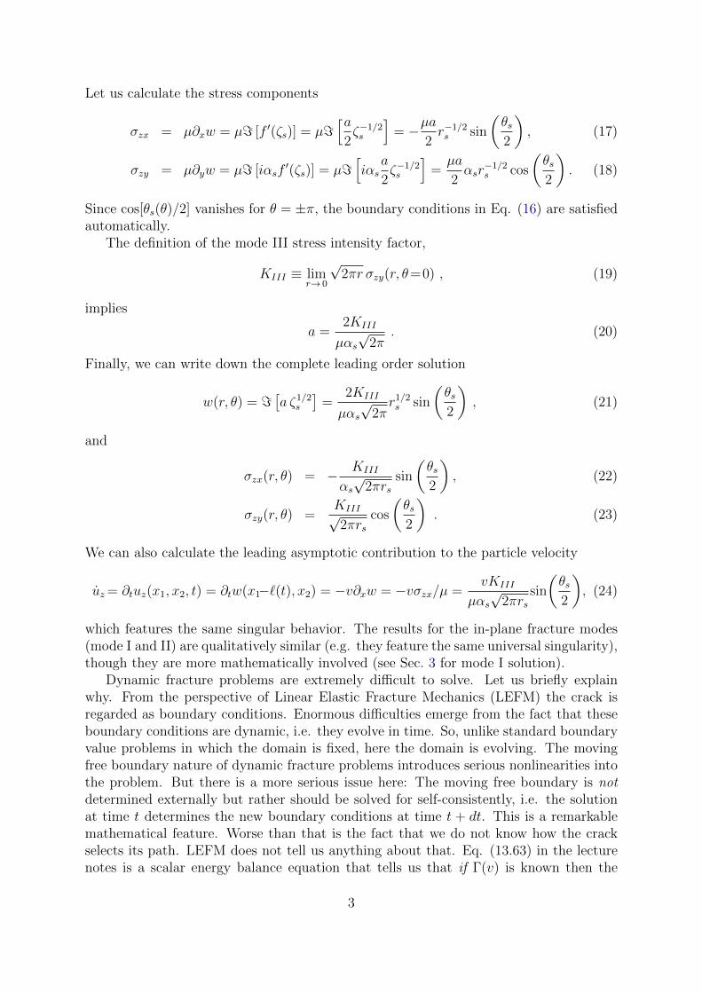
Let us calculate the stress components

σzx = µ∂xw = µ= [f ′(ζs)] = µ=[a

2ζ−1/2s

]= −µa

2r−1/2s sin

(θs2

), (17)

σzy = µ∂yw = µ= [iαsf′(ζs)] = µ=

[iαs

a

2ζ−1/2s

]=µa

2αsr

−1/2s cos

(θs2

). (18)

Since cos[θs(θ)/2] vanishes for θ = ±π, the boundary conditions in Eq. (16) are satisfiedautomatically.

The definition of the mode III stress intensity factor,

KIII ≡ limr→ 0

√2πr σzy(r, θ=0) , (19)

implies

a =2KIII

µαs√

2π. (20)

Finally, we can write down the complete leading order solution

w(r, θ) = =[a ζ1/2

s

]=

2KIII

µαs√

2πr1/2s sin

(θs2

), (21)

and

σzx(r, θ) = − KIII

αs√

2πrssin

(θs2

), (22)

σzy(r, θ) =KIII√2πrs

cos

(θs2

). (23)

We can also calculate the leading asymptotic contribution to the particle velocity

uz= ∂tuz(x1, x2, t) = ∂tw(x1−`(t), x2) = −v∂xw = −vσzx/µ =vKIII

µαs√

2πrssin

(θs2

), (24)

which features the same singular behavior. The results for the in-plane fracture modes(mode I and II) are qualitatively similar (e.g. they feature the same universal singularity),though they are more mathematically involved (see Sec. 3 for mode I solution).

Dynamic fracture problems are extremely difficult to solve. Let us briefly explainwhy. From the perspective of Linear Elastic Fracture Mechanics (LEFM) the crack isregarded as boundary conditions. Enormous difficulties emerge from the fact that theseboundary conditions are dynamic, i.e. they evolve in time. So, unlike standard boundaryvalue problems in which the domain is fixed, here the domain is evolving. The movingfree boundary nature of dynamic fracture problems introduces serious nonlinearities intothe problem. But there is a more serious issue here: The moving free boundary is notdetermined externally but rather should be solved for self-consistently, i.e. the solutionat time t determines the new boundary conditions at time t + dt. This is a remarkablemathematical feature. Worse than that is the fact that we do not know how the crackselects its path. LEFM does not tell us anything about that. Eq. (13.63) in the lecturenotes is a scalar energy balance equation that tells us that if Γ(v) is known then the

3

crack growth rate is known, but there is no information about the direction of growth.Finally, we would like to mention that dynamic fracture is extremely challenging from anexperimental perspective. Take your window glass as an example. The size of the singularregion is in the nanometer scale. The typical crack propagation speed is kilometers persecond. It is impossible today, and most probably in the near future, to probe suchlengthscales at such rates.

1.1 Properties of the solution

1. In the limit of small velocities, v cs, we want to recover the static field we knowfrom the Inglis crack solutions (recall TA #8). Looking at Eqs. (22)-(23), andtaking the limit αs→1, rs→ r, and θs→θ, we find that the results agree with theInglis solution, if we recognise KIII =

√8πLσ∞, where σinf is the far field loading

and L is the size of the crack.

2. Explicit calculation of the J-integral gives:

G(v) =K2III

2µαs≡ AIII(v)

K2III

2µ. (25)

The function AIII(v) is universal, i.e. independent of the geometry and loading of agiven crack problem. As before, all of the details of a given problem are introducedby a single non-universal number, KIII .

3. AI(v) clearly diverges as v approaches cs. What happens with G? Since energybalance implies G(v) = Γ(v) for all velocities, and since Γ(v) is obviously finite, wesee from this analysis that KIII should be (and indeed is) velocity dependent. Thiscompensates for this divergence so as to allow the equality for all velocities.

2 The J-integral

There is one important class of situations in which G (and J) are independent of thepath (contour) C for any C, irrespective of whether it is inside or outside the universalsingular region (= K-field). This happens for steady state crack propagation, i.e. whenv is time-independent. Let us prove it.

2.1 Momentum-energy balance as a continuity equation

Before we start, we note that since the J-integral measures energy flux into the crack,we want to present our equation of motion as a continuity equation for the elastic andkinetic energy. The generic way to do it is to multiply the equation of motion ∇x·σ=ρ vby ui and sum over the index i. In linear elasticity this reads

ρuiui =∂σij∂xj

ui . (26)

The left-hand-side is exactly the time derivative of the kinetic energy T :

ρuiui = ∂t

(1

2ρuiui

)=∂T

∂t, (27)

4

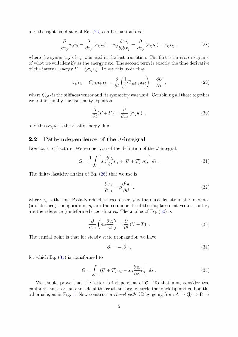
and the right-hand-side of Eq. (26) can be manipulated

∂

∂xjσijui =

∂

∂xj(σijui)− σij

∂2ui∂t∂xj

=∂

∂xj(σijui)− σij εij , (28)

where the symmetry of σij was used in the last transition. The first term is a divergenceof what we will identify as the energy flux. The second term is exactly the time derivativeof the internal energy U = 1

2σijεij. To see this, note that

σij εij = Cijklεijεkl =∂

∂t

(1

2Cijklεijεkl

)=∂U

∂T, (29)

where Cijkl is the stiffness tensor and its symmetry was used. Combining all these togetherwe obtain finally the continuity equation

∂

∂t(T + U) =

∂

∂xj(σijui) , (30)

and thus σijui is the elastic energy flux.

2.2 Path-independence of the J-integral

Now back to fracture. We remind you of the definition of the J integral,

G =1

v

∫C

[sij∂ui∂tnj + (U + T ) vnx

]ds . (31)

The finite-elasticity analog of Eq. (26) that we use is

∂sij∂xj

= ρ∂2ui∂t2

, (32)

where sij is the first Piola-Kirchhoff stress tensor, ρ is the mass density in the reference(undeformed) configuration, ui are the components of the displacement vector, and xjare the reference (undeformed) coordinates. The analog of Eq. (30) is

∂

∂xj

(sij∂ui∂t

)=

∂

∂t(U + T ) . (33)

The crucial point is that for steady state propagation we have

∂t = −v∂x , (34)

for which Eq. (31) is transformed to

G =

∫C

[(U + T )nx − sij

∂ui∂x

nj

]ds . (35)

We should prove that the latter is independent of C. To that aim, consider twocontours that start on one side of the crack surface, encircle the crack tip and end on theother side, as in Fig. 1. Now construct a closed path ∂Ω by going from A → 1© → B →

5

AB C

D

x

y

1

2O

Figure 1: Two contours that start on one side of the crack surface and end on the otherside.

C → 2© → D → A, where the two segments B → C and D → A lie along the two crackfaces. Note that we traverse contour 2© in the opposite direction.

Denoting the area enclosed in ∂Ω by Ω, the proof is as follows

∫∂Ω

(U + T )nxds =

∫Ω

∂

∂x(U + T ) dA = −v−1

∫Ω

∂

∂t(U + T ) dA

= −v−1

∫Ω

∂

∂xj

(sij∂ui∂t

)dA =

∫Ω

∂

∂xj

(sij∂ui∂x

)dA =

∫∂Ω

sij∂ui∂x

njds .

(36)

This implies ∫∂Ω

[(U + T )nx − sij

∂ui∂x

nj

]ds = 0 , (37)

which completes the proof. To understand why, recall that the two segments that liealong the crack faces do not contribute to the integral of Eq. (37) because there we havenx=0 and sijnj =0 (due to the traction-free boundary conditions). This implies that thesum of the two line integrals over contours 1© and 2© vanishes, and since 2© was traversedin the opposite direction, the integrals over 1© and 2© are equal. Since the contours weregeneral, we can conclude that for every path that starts at the lower crack face, encirclesthe tip in the counterclockwise direction, and ends at the upper crack face, the value ofthe integral is the same.

In particular, this result is valid for quasi-static cracks. Though the ideas aboutconfigurational forces were developed by Eshelby in the early 1950’s, the integral discussedabove in the context of fracture theory was independently derived by Cherepanov (1967)and Rice (1968) for quasi-static cracks and then extended to the dynamic case in the1970’s.

6

2.3 Example of usage

Consider the system described in Fig. 2: a plane-stress linear elastic strip (with Young’smodulus E and Poisson’s ratio ν) spanning −∞ < x <∞ and −H < y < H, containinga semi-infinite crack propagating along y = 0 at a speed v. The strip is loaded as follows

uy(x, y=±H, t) = ±δ and ux(x, y=±H, t) = 0 . (38)

Figure 2: Strip with crack

Let’s try to calculate the energy release rate into the crack tip region using theJ-integral. In steady-state propagation we can use the fact that the integral is path-independent and we can choose a convenient contour, that is, a path such that most of itwill give simple contributions to the integral. The contour we choose is shown in Fig. 3,where we take the lateral parts of the contour (i.e. segments 1©, 3© and 5©) to x = ±∞.

Figure 3: The integration contour.

The integration is very easy along this path: Along the segments 1© and 5© boththe stress field and the velocity vanish (why?), therefore they do not contribute. Alongsegments 2© and 4© nx is zero, and u is constant, so they too vanish. Thus, the onlycontribution comes from segment 3©, and it equals 2UH, because u goes to a constantand T vanishes.

The physical picture here is simple and neat: a piece of material at x→∞ is staticallystretched with energy density U . After the crack passes, when the same piece of materialapproaches x → −∞ it releases all its energy and is completely stress free. Where didthe energy go to? To the only place in the theory that can have dissipation, which isthe process zone at the crack tip. Therefore the energy release rate at steady state, J , is

7

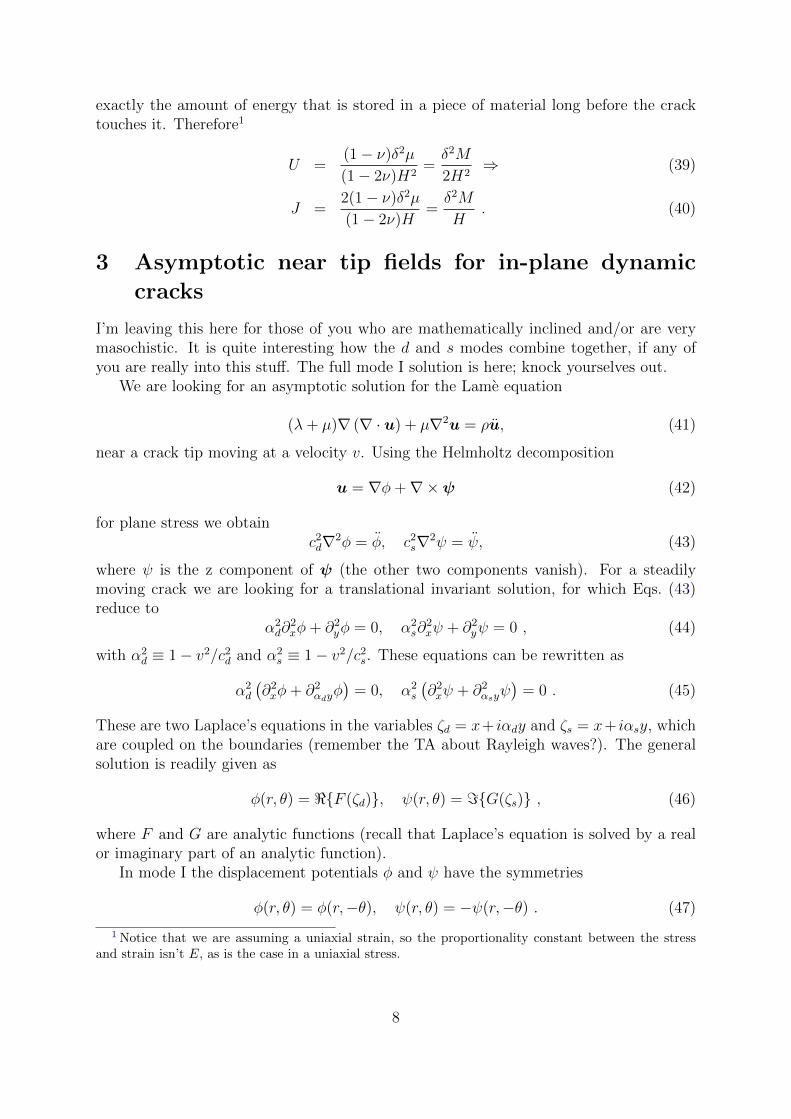
exactly the amount of energy that is stored in a piece of material long before the cracktouches it. Therefore1

U =(1− ν)δ2µ

(1− 2ν)H2=δ2M

2H2⇒ (39)

J =2(1− ν)δ2µ

(1− 2ν)H=δ2M

H. (40)

3 Asymptotic near tip fields for in-plane dynamic

cracks

I’m leaving this here for those of you who are mathematically inclined and/or are verymasochistic. It is quite interesting how the d and s modes combine together, if any ofyou are really into this stuff. The full mode I solution is here; knock yourselves out.

We are looking for an asymptotic solution for the Lame equation

(λ+ µ)∇ (∇ · u) + µ∇2u = ρu, (41)

near a crack tip moving at a velocity v. Using the Helmholtz decomposition

u = ∇φ+∇×ψ (42)

for plane stress we obtainc2d∇2φ = φ, c2

s∇2ψ = ψ, (43)

where ψ is the z component of ψ (the other two components vanish). For a steadilymoving crack we are looking for a translational invariant solution, for which Eqs. (43)reduce to

α2d∂

2xφ+ ∂2

yφ = 0, α2s∂

2xψ + ∂2

yψ = 0 , (44)

with α2d ≡ 1− v2/c2

d and α2s ≡ 1− v2/c2

s. These equations can be rewritten as

α2d

(∂2xφ+ ∂2

αdyφ)

= 0, α2s

(∂2xψ + ∂2

αsyψ)

= 0 . (45)

These are two Laplace’s equations in the variables ζd = x+ iαdy and ζs = x+ iαsy, whichare coupled on the boundaries (remember the TA about Rayleigh waves?). The generalsolution is readily given as

φ(r, θ) = <F (ζd), ψ(r, θ) = =G(ζs) , (46)

where F and G are analytic functions (recall that Laplace’s equation is solved by a realor imaginary part of an analytic function).

In mode I the displacement potentials φ and ψ have the symmetries

φ(r, θ) = φ(r,−θ), ψ(r, θ) = −ψ(r,−θ) . (47)

1 Notice that we are assuming a uniaxial strain, so the proportionality constant between the stressand strain isn’t E, as is the case in a uniaxial stress.

8

For these symmetries to hold, we need to demand that F and G will have the followingsymmetries:

F (ζ) = F (ζ), G(ζ) = G(ζ) . (48)

To see that these requirements ensure the symmetries of Eq. (47), note that Eqs. (48)simply imply that the coefficients of the Laurent expansions of F and G (the complexgeneralization of the Taylor expansion of real functions) are all real. Writing now ζd =rde

iθd and ζs = rseiθs we see that φ in Eq. (46) picks up the cosines and ψ picks up the

sines, as required.To determine F and G we should impose the free boundary conditions on the crack

facesσyy(r, θ = ±π) = σxy(r, θ = ±π) = 0 . (49)

These components are written in terms of φ and ψ as

σyy(r, θ) = µ

[c2d

c2s

∇2φ− 2∂xxφ− 2∂xyψ

]σxy(r, θ) = µ [2∂xyφ+ ∂yyψ − ∂xxψ] .

(50)

The second derivatives of φ and ψ, in terms of F and G, are

∂xxφ = <[F ′′(ζd)], ∂xxψ = =[G′′(ζs)],

∂yyφ = <[−α2dF′′(ζd)], ∂yyψ = =[−α2

sG′′(ζs)],

∂xyφ = <[iαdF′′(ζd)], ∂xyψ = =[iαsG

′′(ζs)] .

(51)

Substituting into Eqs. (50) we obtain

σyy(r, θ) = −µ<[(1 + α2

s)F′′(ζd) + 2αsG

′′(ζs)]

σxy(r, θ) = −µ=[2αdF

′′(ζd) + (1 + α2s)G

′′(ζs)].

(52)

Note that the polar coordinates r, θ are related to rd,s, θd,s according to

rd = r√

1− (v sin θ/cd)2, tan θd = αd tan θ,

rs = r√

1− (v sin θ/cs)2, tan θs = αs tan θ .

We are now ready to solve the problem in a power series. The leading term in theexpansion of σ is a square root, i.e.

F ′′(ζ) = aζ−1/2, G′′(ζ) = bζ−1/2 , (53)

where a/b will be determined by the boundary conditions of Eq. (49). SubstitutingEq. (53) into Eqs. (52), we obtain

σyy(r, θ) = −µ[(1 + α2

s)ar−1/2d cos(θd/2) + 2αsbr

−1/2s cos(θs/2)

]σxy(r, θ) = µ

[2αdar

−1/2d sin(θd/2) + (1 + α2

s)br−1/2s sin(θs/2)

].

(54)

Noting thatrd,s(θ = ±π) = r, θd,s(θ = ±π) = ±π , (55)

9

we observe that in Eqs. (52) σyy(r,±π) vanishes identically for any a and b and thatσxy(r,±π) vanishes only if

a = (1 + α2s)A, b = −2αdA . (56)

A is some undetermined prefactor that will be related to the stress intensity factor. Toproceed, by double integration (omitting terms that do not affect stress/strain) we readilyobtain

F (ζ) = (1 + α2s)

4Aζ3/2

3, G(ζ) = −2αd

4Aζ3/2

3. (57)

The stresses are then obtained by replacing Eq. (56) into (54):

σyy(r, θ) = −µA[(1 + α2

s)2r−1/2d cos(θd/2)− 4αsαdr

−1/2s cos(θs/2)

]σxy(r, θ) = µA

[2αd(1 + αs)

2r−1/2d sin(θd/2)− 2(1 + α2

s)αdr−1/2s sin(θs/2)

].

(58)

The stress intensity factor is defined as

KI = limr→ 0

√2πr σyy(r, θ=0; v) (59)

and hence

A =KI

µD(v)√

2π, (60)

whereD(v) = 4αsαd − (1 + α2

s)2 (61)

is the Rayleigh function (the very same function as Eq. (27) from TA#6 about Rayleighwaves. It vanishes at v = cR).

Collecting everything, we end up with

ux(r, θ) =2KI

µ√

2πD(v)

[(1 + α2

s)r1/2d cos

(θd2

)− 2αdαsr

1/2s cos

(θs2

)],

uy(r, θ) =− 2KIαd

µ√

2πD(v)

[(1 + α2

s)r1/2d sin

(θd2

)− 2r1/2

s sin

(θs2

)].

(62)

3.1 Properties of the solution

1. In the limit of small velocities, v cs, we want to recover the static field presentedin the lecture notes. However, this is not so simple. Look at the numerator of ux inEq. (62): when v → 0, we have αi → 1 and ri → r so the numerator goes to zero.Luckily, the Rayleigh function D(v) also goes to zero, and they do so at the samerate of v2 (it is easily shown that both D(v) and the numerator of ux go as v2 toleading order in v, since they depend on v only through functions of v2).

2. From the stress field, we can calculate the hoop stress σθθ. It turns out that itdepends on velocity in an interesting manner, as seen in this figure (from Freund1990):

10

One sees that for v ∼ 0.6cs the maximal hoop stress occurs for θ = 0 which iswhat we would expect. However, at higher velocities there seems to be a “firstorder phase transition” where the maximum jumps to a finite angle, around 60.This was first noticed by Yoffe (1951) and was suggested as a mechanism for thebranching instability. the angle between bifurcating cracks is generically much lessthan 60 and anyhow we already know that this theory cannot tell us how thingsbreak because the theory fails at the process zone.

3. Explicit calculation of the J-integral gives:

G(v) =v2αdK

2I

2µc2sD(v)

≡ AI(v)K2I

E. (63)

The function AI(v) is universal, i.e. independent of the geometry and loading of agiven crack problem. As before, all of the details of a given problem are introducedby a single non-universal number, KI .

4. In the limit v → 0 we have AI(v) → 1, and then Eq. (63) coincides with thequasi-static problem that we solved in class.

5. Since D(cR) = 0, AI(v) clearly diverges as v approaches the Rayleigh velocity.What happens with G? Since energy balance implies G(v) = Γ(v) for all velocities,and since Γ(v) is obviously finite, we see from this analysis that KI should be (andindeed is) velocity dependent. This compensates for this divergence so as to allowthe equality for all velocities.

11