1 motivation - cce.pk.edu.pl
TRANSCRIPT

Computer Methods in Civil Engineering
lecture notes by Witold Cecot
June 15, 2021
1 Motivation
US Government study: ”... modeling and simulation are emerging as key technolo-gies to support manufacturing in the 21st century, and no other technology offers
more potential than modeling and simulation for improving products, perfecting pro-cesses, reducing design-to-manufacturing cycle time, and reducing product realiza-
tion costs...”.The Finite Element Method (FEM), which is the most popular modeling
tool, is a very successful story. It is a way that engineers invented to solve equationsof mechanics to find displacements and stresses in structures. The history of FEM
begins in 1915 with B. Galerkin who used 2-3 sophisticated trial functions. In40’s A. Hrennikoff and R. Courant had two different conceptions but the commonkey point to use many simple trial functions. First developments of the method
are associated with the following names: J. Argyris, M. Turner, R. Clough (whocoined the terminology finite element method) and O. Zienkiewicz.
Mathematicians contributed to understanding as well as the reliability of FEM.For many problems, FEM analysis is an art.
• FEM makes a good engineer great, and a bad engineer dangerous (R.Cook).
• Modeling (simulating nature) gives us insight into the world we live in.
• An engineer has to know how to: assume a model, solve it on a laptop, andassess the results.
1

2 General idea of the finite element method
1. Let’s consider the Laplace PDE equation (as a model of e.g. stationary heat transfer)
u(x, y) ∈ C2(Ω) : R2 ⊃ Ω→ R
−k∆u = f(x, y) in Ω
u = u on ∂ΩD
k ∂u∂n
= t on ∂ΩN
(1)
2. Weak formulation (”virtual work principle”) of the Laplace problem:
Find continuous u(x, y) ∈ H1(Ω) + u, such that u = u on ∂ΩD and
∫
Ω
k∇v · ∇u dx dy =
∫
Ω
vf dx dy +
∫
∂ΩN
vtdγ ∀v ∈ H10 (2)
3. FEM (Galerkin’s method with solution approximation by shape functions)
• Domain (with heat source f = 60 for x > 1, all quantities are dimensionless) and itsdiscretization with 2 finite elements (4 nodes)
A
B
CDu = 3x− 2
t1 = 0
t2 = 18xt3 = 0
0 0.5 1 1.5 2
−1.2
−1
−0.8
−0.6
−0.4
−0.2
0
0.2
1 2
0 0.5 1 1.5 2
−1.2
−1
−0.8
−0.6
−0.4
−0.2
0
0.2
1 2 3
4
• Selected shape functions - ϕ1(x, y), ϕ2(x, y)
• Continuous approximation of the solutionuh(x, y) = α1ϕ1(x, y) + α2ϕ2(x, y) + α3ϕ3(x, y) + α4ϕ4(x, y)
α1, α2, . . . αN - unknown parameters - degrees of freedom (d.o.f.)
2

• Galerkin’s methodv ∈ ϕ1, ϕ2, ϕ3, ϕ4 ⇒4 algebraic equations - ”virtual work” for ”virtual” displacements ϕ1, ϕ2, ϕ3, ϕ4
Let’s assume the following notations:
(ϕi, ϕj)m = αj
∫
emk∇ϕi · ∇ϕj dx dy
(ϕi)m =∫
emϕif dx dy +
∫
∂ΩN∩∂emϕit ds
(ϕ1, ϕ1)1 +(ϕ1, ϕ1)2 +(ϕ1, ϕ2)1 +(ϕ1, ϕ2)2 +(ϕ1, ϕ3)1 +(ϕ1, ϕ3)2 +(ϕ1, ϕ4)1 +(ϕ1, ϕ4)2 = (ϕ1)1 +(ϕ1)2
(ϕ2, ϕ1)1 +(ϕ2, ϕ1)2 +(ϕ2, ϕ2)1 +(ϕ2, ϕ2)2 +(ϕ2, ϕ3)1 +(ϕ2, ϕ3)2 +(ϕ2, ϕ4)1 +(ϕ2, ϕ4)2 = (ϕ2)1 +(ϕ2)2
(ϕ3, ϕ1)1 +(ϕ3, ϕ1)2 +(ϕ3, ϕ2)1 +(ϕ3, ϕ2)2 +(ϕ3, ϕ3)1 +(ϕ3, ϕ3)2 +(ϕ3, ϕ4)1 +(ϕ3, ϕ4)2 = (ϕ3)1 +(ϕ3)2
(ϕ4, ϕ1)1 +(ϕ4, ϕ1)2 +(ϕ4, ϕ2)1 +(ϕ4, ϕ2)2 +(ϕ4, ϕ3)1 +(ϕ4, ϕ3)2 +(ϕ4, ϕ4)1 +(ϕ4, ϕ4)2 = (ϕ4)1 +(ϕ4)2
(3)Entries in gray are equal to 0. Entries in red and green are integrals over elements 1 and2 respectively.
• m-th element (stiffness) matrix and (load) vector
Kmij =
∫
emk∇ϕi · ∇ϕj dx dy, fm
i =∫
emϕif dx dy +
∫
∂ΩN∩∂emϕit ds
• After assembling (element by element) one obtains global system of 4× 4 algebraic linearequations Ku = f .
• Accounting for Dirichlet (essential, kinematic) boundary conditions
e.g. if u = 3x− 2 is given at segment AD it implies that α1 = −2, α2 = 1Therefore, equations 1 and 2 are not needed.
• Postprocessing (performed element by element, with possible assessment of the resultquality).
For element 1: d.o.f. (α1, α2, α4) are already known, thus one may evaluate in thiselement
approximation of solution: uh(x, y) = α1ϕ1(x, y) + α2ϕ2(x, y) + α4ϕ4(x, y)
and flux approximation: qh = −k[α1∇ϕ1(x, y) + α2∇ϕ2(x, y) + α4∇ϕ4(x, y)]
In general, uh is continuous but qh is not and the accuracy of uh is worse than uh accuracy.”Reaction” (normal component of flux) at the AD edge: qn = qh · n
3

4

4. Homework
Consider problem (1) in the domain shown in this section (item 3).
• Write the formulas for FEM approximation of the solution, its flux and qn along the ADsegment, knowing that α3 = 2, α4 = −2/3.• Prove that such an approximation is continuous and satisfies the Dirichlet boundary con-dition. Evaluate α1, α2 for u = x2
• Check accuracy of stisfying the Neumann b.c. if t1 = −1, t2 = 0, t3 = 1− x
5
3 Higher order finite element approximation
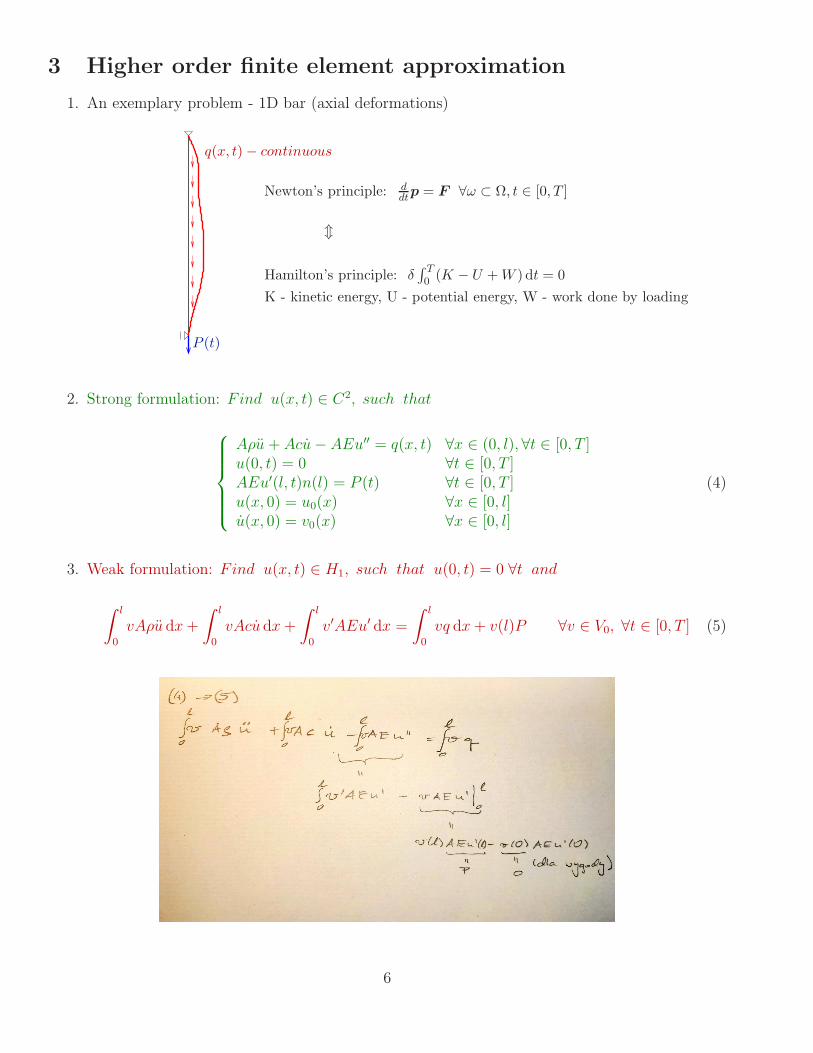
1. An exemplary problem - 1D bar (axial deformations)
q(x, t)− continuous
P (t)
Newton’s principle: ddtp = F ∀ω ⊂ Ω, t ∈ [0, T ]
m
Hamilton’s principle: δ∫ T0 (K − U +W ) dt = 0
K - kinetic energy, U - potential energy, W - work done by loading
2. Strong formulation: Find u(x, t) ∈ C2, such that
Aρu + Acu− AEu′′ = q(x, t) ∀x ∈ (0, l), ∀t ∈ [0, T ]u(0, t) = 0 ∀t ∈ [0, T ]AEu′(l, t)n(l) = P (t) ∀t ∈ [0, T ]u(x, 0) = u0(x) ∀x ∈ [0, l]u(x, 0) = v0(x) ∀x ∈ [0, l]
(4)
3. Weak formulation: Find u(x, t) ∈ H1, such that u(0, t) = 0 ∀t and
∫ l
0
vAρu dx+
∫ l
0
vAcu dx+
∫ l
0
v′AEu′ dx =
∫ l
0
vq dx+ v(l)P ∀v ∈ V0, ∀t ∈ [0, T ] (5)
6

4. FEM (Galerkin’s method and solution approximation by shape functionsLet’s assume that u = 0 ∀t. Then u = u(x).
7

• Discretization (finite elements)
• Shape functions (e.g. on element 3, using local enumeration)element by element algorithm
ϕ1(x) =(x− x2)(x1 − x2)
, ϕ2(x) =(x− x1)(x2 − x1)
, ϕ3(x) = (x− x1)(x− x2)
remarks: ϕ1(x) + ϕ2(x) = 1, ϕ1(x) + ϕ2(x) + ϕ3(x) 6= 1position of the third node is neither specified nor used
• Approximation of a solution (over element 3)uh(x) = α1ϕ1(x) + α2ϕ2(x) + α3ϕ3(x), d.o.f. α1, α2, α3 - degrees of freedom (d.o.f.)
α1 = uh(x1), α2 = uh(x2)
• Approximation of the geometry (on element 3)
8

1 2 3
1 2 3 4 5 6
1
1
1
2
23
2 3
x = x1ϕ1(x) + x2ϕ2(x)
• Galerkin’s method
∫ l
0
ϕ′iAEu
′h dx =
∫ l
0
ϕiq dx+ ϕi(l)P ∀ϕi, i = 1, ..., N (6)
• Element stiffness matrix and load vectorKe
ij =∫
eϕ′iAEϕ
′j dx, Pi =
∫
eϕiq dx
or in a matrix form (for a 2 dof element)Ke =
∫
eBTDB dx, B = [ϕ′
1 ϕ′2 ϕ
′3], D = AE
P e =∫
eNT q dx, N = [ϕ1 ϕ2 ϕ3]
• Assembling
• Accounting for kinematic conditions
• SLE solution; Ku = P (+F ); F - nodal forces for bar structures only
• Postprocessing with assesment of the result quality
e.g. for element 3, d.o.f. (α1, α2, α3) are already known, thus
continuous approximation of axial displacement: uh(x) = α1ϕ1(x) + α2ϕ2(x) + α3ϕ3(x)
discontinuous approximation of axial stress: σh(x) = E duh
dx= α1ϕ
′1(x)+ α2ϕ
′2(x)+ α3ϕ
′3(x)
discoountinuous approximation of axial force: Sh(x) = Aσh(x)
improved (in fact exact) axial nodal values of axial forces: F e =Keue − P e
• HomeworkConsider the following 1D bar problemFind u(x) ∈ H1([a, b]), such that u(a) = u(b) = 0 and
∫ b
a
v′AEu′ dx =
∫ b
a
vq0(l − x) dx ∀v ∈ V0, q0 ∈ R, l = b− a (7)
9

– Calculate the matrix and vector for the three node finite element [2,3] with hierarchicalshape functions up to the second order.
– Assemble the matrix and vector assuming that the global node numbers are 1,3,2(left, mid, right).
– Write the formulas used for FEM approximation of axial displacement and axial forceover that element.
– Discretize a bar represented by segment [1,3] with 2 second order hierarchical elements.
– Calculate FEM approximation of the axial force and the improved axial forces.
– Check the global equilibrium equation.
4 FEM analysis of mechanical vibrations
Vibrations - incredible common phenomenon. In certain cases they are a positive thing (speech,music) and sometimes a negative one (noise of braking pads, vibration of buildings, bridges,...).Engineers are involved in both making and suppressing vibrations.
1. Types of the related problems
• Eigen vibrations.
• Response to time dependent loading (periodic or random).
• Wave propagation.
2. Single DOF system - without external excitation
m
ck
x
mx+ cx+ kx = 0 ∀t ∈ (0, τ)x(0) = x0x(0) = v0
δ = c2m, ζ = δ
ω- damping ratio
α1,2 = ω(−ζ ±√
ζ2 − 1) ∈ C, x = A1ea1t + A2e
a2t, eiθ = cos(θ) + i sin(θ)
• ζ = 0 → mx+ kmx = 0 → x = A sin(ωt− ϕ) or x = A sin(ωt) +B cos(ωt)
−mAω2cos(ωt− ϕ) + kAcos(ωt− ϕ) = 0
kA = ω2mA, → A 6= 0, ω =√
km
- natural (angular) frequency
initial conditions imply A (amplitude) and ϕ (phase), but typically they are not important
• 0 < ζ 6 1 → x = Ae−ζωt cos(ωdt− ϕ),ωd = ω
√
1− ζ2 - damped natural ’frequency’experimental estimation of damping ratio: ζ ≈ 0.11
n50%
10

• 1 < ζ → x = A1eα1ωt + A2e
α2ωt,α1, α2, ω ∈ R
0 0.5 1 1.5 2−0.2
−0.15
−0.1
−0.05
0
0.05
0.1
0.15
0.2
t
cos(20 t)/10 + sin(20 t)/10
0 0.5 1 1.5 2−0.5
−0.4
−0.3
−0.2
−0.1
0
0.1
0.2
0.3
0.4
0.5
t
(4 71/2
sin((15 71/2
t)/2))/(21 exp((5 t)/2))
0 0.5 1 1.5 2−0.2
−0.15
−0.1
−0.05
0
0.05
0.1
0.15
0.2
t
1/(3 exp(10 t)) − 1/(3 exp(40 t))
3. Axial vibrations of elastic bars
A,E,ρ
l
longitudinal wave
particles vibrate in the direction of wave propagation
u - particle vibration, u = u(x, t)
wave propagation
4. Axial free vibrations of elastic barsStanding (stationary, fixed in space) waves - combination (interference) of two waves movingin opposite directions, each having the same amplitude and frequency. When waves are super-imposed, their energies are either added together or cancelled out. The PDE of motion reducesin this case to the following problem.
ρu− Eu′′ = 0 ∀x ∈ (0, l), ∀t ∈ [0, τ ] wave (string) equationu(0, t) = 0 ∀t ∈ [0, τ ]u′(l, t) = 0 ∀t ∈ [0, τ ]
(8)
Separation of variables, u(x, t) = U(x)V (t) implies U ′′
U= V
VρE= const and results in two
eigenproblems (the Helmholtz equations)
V + ω2nV = 0
U ′′ + k2nU = 0(9)
where kn = ωn
√
ρEare wave numbers and the general, nontrivial solution is of the form
u(x, t) =∞∑
n=1
[An cos(ωnt) +Bn sin(ωnt)] [(Cn cos(knx) +Dn sin(knx)], (10)
ωn = 2πfn, ωn = 2πTn, kn = 2π
λn, λn
Tn= ωn
kn=
√
Eρ− sound (phase) speed
The Dirichlet b.c. implies that Cn = 0
The Neumann b.c. implies the characteristic equation
cos(knl) = 0 ⇒ knl = (2n− 1)π
2, n = 1, 2, 3, . . . (11)
11
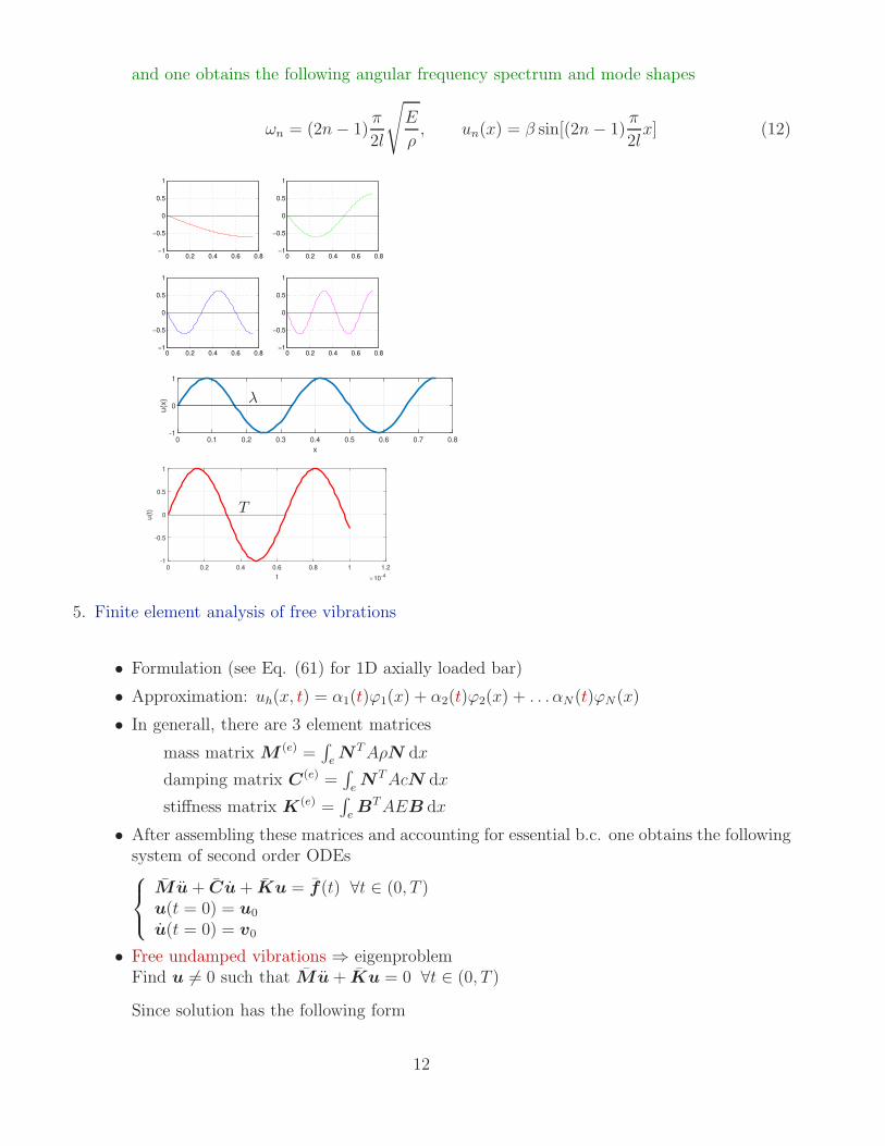
and one obtains the following angular frequency spectrum and mode shapes
ωn = (2n− 1)π
2l
√
E
ρ, un(x) = β sin[(2n− 1)
π
2lx] (12)
0 0.2 0.4 0.6 0.8−1
−0.5
0
0.5
1
0 0.2 0.4 0.6 0.8−1
−0.5
0
0.5
1
0 0.2 0.4 0.6 0.8−1
−0.5
0
0.5
1
0 0.2 0.4 0.6 0.8−1
−0.5
0
0.5
1
0 0.1 0.2 0.3 0.4 0.5 0.6 0.7 0.8
x
-1
0
1
u(x
) λ
0 0.2 0.4 0.6 0.8 1 1.2
t 10-4
-1
-0.5
0
0.5
1
u(t
) T
5. Finite element analysis of free vibrations
• Formulation (see Eq. (61) for 1D axially loaded bar)
• Approximation: uh(x, t) = α1(t)ϕ1(x) + α2(t)ϕ2(x) + . . . αN(t)ϕN(x)
• In generall, there are 3 element matrices
mass matrix M (e) =∫
eNTAρN dx
damping matrix C(e) =∫
eNTAcN dx
stiffness matrix K(e) =∫
eBTAEB dx
• After assembling these matrices and accounting for essential b.c. one obtains the followingsystem of second order ODEs
Mu+ Cu+ Ku = f(t) ∀t ∈ (0, T )u(t = 0) = u0
u(t = 0) = v0
• Free undamped vibrations ⇒ eigenproblemFind u 6= 0 such that Mu+ Ku = 0 ∀t ∈ (0, T )
Since solution has the following form
12

u = U sin(ωt+ ψ)
one obtains(−ω2MU + KU) sin(ωt+ ψ) = 0 ∀t ∈ (0, T )
that reduces to the following generalized algebraic eigenproblem
KU = ω2MU
UTMU = µ0, µ0 is an arbitary constant, e.g. 1 kg(13)
which, in turn, enables computation of approximate mode shapes (U 1,U 2, . . .) and cor-responding natural frequencies (ω1, ω2, . . .)
• Due to the symmetry of M and K the eigen modes are orthogonal, i.e.
UTi MU j = 0 for i 6= j
UTi KU j = 0 for i 6= j
UTk MU k = 1 UT
k KU k = ω2k (for normalized U k)
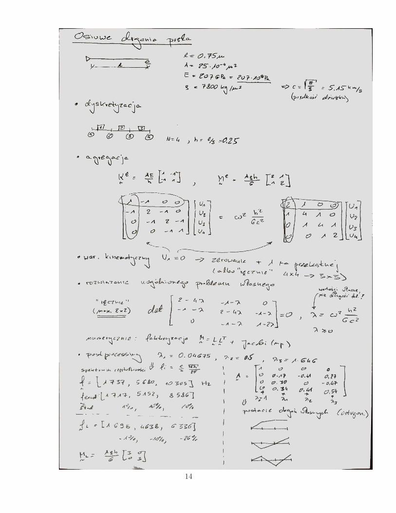
• example
13
14

6. Numerical integration in time
For the initial value problem dydt
= f, y(t0) = y0
one introduces discretization in time represented by time step t.
15

Thus, y(t0 +t) = y0 +
∫ t0+t
t0
f dt
The last integral is evaluated after assuming an approximation for integrand f , that is equiva-lent to assuming certain approximation of y with respect to time.
7. Types of numerical methods for integration in time
• Single-step and multi-step.
• Explicit and implicit.
• Conditionally or unconditionally stable.
8. Newmark’s method (for β = 0.5, γ = 1)Without damping Mu+ Ku = f(t) ∀t ∈ (0, T )
• For given: u0, v0, Ma0 = f0 − Ku0
• (M + 12t2K)ak+1 = fk+1 − K(uk +tvk)
• uk+1 = uk +tvk + 12t2ak+1
• vk+1 = vk +tak+1
9. Modal analysis ( a good approximation for harmonic response)
• u = z1(t)U 1 + z2(t)U 2 + . . .+ zN (t)UN , U i - eigen vectors
• zi + ζizi + ω2i zi = Fi, ζi = α + βω2
i ∀i = 1, ..., N (decoupled system of ODEs)
10. Fourier analysis
• Fourier series for a periodic function (T = 2l):
FS(f)(x) = a0 +
n=∞∑
n=1
(
an cosnπx
l+ bn sin
nπx
l
)
=
n=∞∑
n=−∞
Cneinπx/l
where
an =1
l
∫ l
−l
f(x) cosnπx
ldx, a0 =
1
2l
∫ l
−l
f(x) dx
bn =1
l
∫ l
−l
f(x) sinnπx
ldx, Cn =
1
2l
∫ l
−l
f(x)e−inπx/l dx
• nπ
l= ωn, fn =
n
T- sequence of angular frequencies (infinite spectrum)
16

• A function may be represented both in time and frequency domains
TIME domain - f(x) FREQUENCY domain - |Cn|(ωn) (ωn = nπl)
-2 -1.5 -1 -0.5 0 0.5 1 1.5 2
-2.5
-2
-1.5
-1
-0.5
0
0.5
1
1.5
2cos(pi*t)+sqrt(3)*sin(pi*t)-sin(2*pi*t)+1/10*sin(5*pi*t)
2 4 6 8 10 12 14 16 18 200
0.2
0.4
0.6
0.8
1
1.2
1.4
1.6
1.8
2
Ai =√
a2i + b2i
• For non-periodic function (T =∞)Fourier transform to frequency domain
a(ω) =1
π
∫ ∞
−∞
f(x) cos(ωx) dx, b(ω) =1
π
∫ ∞
−∞
f(x) sin(ωx) dx, C(ω) =
∫ ∞
−∞
f(x)e−2πiωx dx
Inverse transform
f(x) =
∫ ∞
−∞
[a cos(ωx) + b sin(ωx)] dω =
∫ ∞
−∞
C(ω)e2πiωx dω
TIME domain - f(x) FREQUENCY domain - C(ω) (ω ∈ R)
−1.5 −1 −0.5 0 0.5 1 1.5−0.5
0
0.5
1
1.5
−10 −5 0 5 10−0.4
−0.2
0
0.2
0.4
0.6
0.8
1
• In practice: DFT, FFT
17

11. Homework
• Use 2 finite elements with linear shape functions for a bar and
– compute global stiffness and mass matrices for such a discretization
– calculate spectrum of natural frequencies and draw the corresponding mode shapes
– verify orthogonality of the modes, calculate modal masses and stiffnesses
– repeat the above proposed analysis for a lumped mass matrix
– Explain differences between single and multi step methods, explicit and implicitschemas, stable and unstable methods.
– Sketch graphs of f(t) = 2 cos(πt)− sin(πt2) in time and frequency domains.
• Knowing that u(x, t) =
∞∑
n=1
[An cos(ωnt) +Bn sin(ωnt)] [(Cn cos(knx) + Dn sin(knx)] is a
general form of the eiegen function (exact free vibration displacements) for a bar clampedat both ends, determine the bar eigen frequencies and eigen modes.
5 Linear elasticity
1. Principle of virtual work (primal weak formulation):
Find continuous u(x, y, z) ∈ H1(Ω) + u, such that u = u on ∂Ωu and
∫
Ω
ε(v) : σ(u) dx dy dz =
∫
Ω
v · f dx dy dz +
∫
∂Ωt
v · t ds ∀v ∈ H10 (14)
σ = Cε (21 independent parameters reduce to 2 for isotropic materials)σij = 2µεij + λδijεkkαεijεij 6 Cijklεijεkl 6 βεijεij , α, β > 0 (positive definitness and elipticity)
2. Plane strain state (3D → 2D), ε33 = 0, σ33 =λ
2(µ+λ)(σ11 + σ22)
x
y
z
dS
Figure 1: Plane strain example. An infinite long body, its section of arbitrary length d and selectedcross section S used for representing the whole body
Find continuous u(x, y) ∈ H1(Ω) + u, such that u = u on ∂Ωu and
18
∫
S
ε(v) : σ(u) dx dy =
∫
S
v · f dx dy +
∫
∂St
v · t ds ∀v ∈ H10 (15)
Even if the assumptions of the plane strain state are not met exactly one may use this simpli-fication of a 3D state being aware of introducing an additional modeling error.
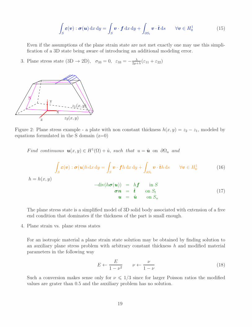
3. Plane stress state (3D → 2D), σ33 = 0, ε33 = − λ2µ+λ
(ε11 + ε22)
x
y
z
S
z1(x, y)
z2(x, y)
Figure 2: Plane stress example - a plate with non constant thickness h(x, y) = z2 − z1, modeled byequations formulated in the S domain (z=0)
Find continuous u(x, y) ∈ H1(Ω) + u, such that u = u on ∂Ωu and
∫
S
ε(v) : σ(u)h dx dy =
∫
S
v · fh dx dy +∫
∂St
v · th ds ∀v ∈ H10 (16)
h = h(x, y)−div(hσ(u)) = hf in S
σn = t on St
u = u on Su
(17)
The plane stress state is a simplified model of 3D solid body associated with extension of a freeend condition that dominates if the thickness of the part is small enough.
4. Plane strain vs. plane stress states
For an isotropic material a plane strain state solution may be obtained by finding solution toan auxiliary plane stress problem with arbitrary constant thickness h and modified materialparameters in the following way
E ← E
1− ν2 ν ← ν
1− ν (18)
Such a conversion makes sense only for ν 6 1/3 since for larger Poisson ratios the modifiedvalues are grater than 0.5 and the auxiliary problem has no solution.
19

5. Fundamental solution in 2D
Gij =1
8πµ(1− ν) [(3− 4ν)lnr + r,i r,j ] (19)
6. Do not use pointwise kinematic boundary conditions in 2D and 3D for problemsof second order!
7. Pointwise loading for these problems is also not reasonable!
8. Solution singularities - an example
Figure 3: Equivalent stress for a plane strain problem. Problem scheme and the Mises equivalentstress distribution with singularity at the reentrant corner and end points of the fixed support
9. Locking example
6 Coupled problem
1. Formulation of a steady-state thermo-mechanical problem (with neglected interior source terms)
Find u ∈H10(Ω) + h and θ ∈ H1
0 + T , such that:
∫
Ω
ε(v) : C ε(u) dΩ−∫
Ω
tr(ε(v))αθ dΩ =∫
∂Ωt
vq ds
∫
Ω
∇ψ k∇θ dΩ =∫
∂Ωs
ψS ds(20)
20
100
102
104
106
108
10−2
10−1
100
101
102
#dof
err
or[
%]
1:100 aspect ratio1:10 aspect ratio
100
102
104
106
108
10−4
10−3
10−2
10−1
#dof
||u
||
1:100 aspect ratio1:10 aspect ratio
h
L
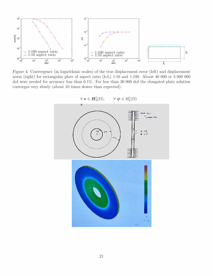
Figure 4: Convergence (in logarithmic scales) of the true displacement error (left) and displacementnorm (right) for rectangular plate of aspect ratio (h:L) 1:10 and 1:100. About 40 000 or 3 000 000dof were needed for accuracy less than 0.1%. For less than 30 000 dof the elongated plate solutionconverges very slowly (about 10 times slower than expected).
∀ v ∈H10(Ω), ∀ ψ ∈ H1
0 (Ω)
21

2. Element stiffness matrix and load vector (N 1 = [ϕ1, 0, 0], N 2 = [0, ϕ1, 0], . . .)
Kuuij =
∫
e
ε(N i) : C ε(N j) dΩ Kuθij =
∫
e
tr(ε(N i))αϕj dΩ (21)
Kθθij =
∫
e
∇ϕi k∇ϕj dΩ (22)
P ui =
∫
∂e∩Ωt
N iq ds (23)
P θi =
∫
∂e∩ΩS
ϕiS ds (24)
3. Assembling element matrices (vectors) into global matrix (vector) - on the basis of d.o.f. con-nectivities (local with global numbering relations)
4. Exemplary 2D domain and discretization by 3 elements
5. Selected scalar (ϕi) vertex and edge shape functions
22

q 1
2
3
4
5
6
7
8
0 0.5 1 1.5 2 2.5 30
0.5
1
1.5
2
2.5
3
0
0.1
0.2
0.3
0.4
0.5
0.6
0.7
0.8
0.9
3 physical elements
0 0.5 1 1.5 2 2.5 30
0.5
1
1.5
2
2.5
3
0
0.1
0.2
0.3
0.4
0.5
0.6
0.7
0.8
0.9
6. Static boundary conditions (only distributed loading is used in well posed problems)Non-zero entries of load vector (using local node numbering) for the triangular element
Pu
4 =
∫
∂e∩Ωt
[0, x/2][0, q(x)]T ds (25)
Pu
6 =
∫
∂e∩Ωt
[0, x(1− x/2)][0, q(x)]T ds (26)
Pu
8 =
∫
∂e∩Ωt
[0, 1− x/2)][0, q(x)]T ds (27)
7. Kinematic boundary conditionsBoth components of displacement along the part of the boundary (x = 0, 1 6 y 6 3) are 0.Never use pointwise kinematic boundary conditions in 2D and 3D problems ofsecond order!
8. Postprocessing
u = Σn1αkN k (continuous)⇒ ε, σ (discontinuous) (28)
9. A’posteriori error estimation and mesh adaptation
Figure 5: Heterogeneous material distribution (colors represent different materials) and hp-adaptedFEM mesh (colors represent order of approximation). Note the ”hanging”.
23

10. Homework
• For the plane strain problem and discretization by 3 elements
– sketch graphs of all shape functions
– calculate load vectors for all elements
– calculate displacements at one interior point of each element for the following d.o.f.[0, 0, 0, 0, 0, 0, 0.5, −1, 1, −2, 1, −2, 2, −3, 2, −2.5]10−2
11. Mixed (the Hellinger-Reissner principle), 2 field
- good coarse mesh accuracy for stresses
- no problems with the incompressible material (ν = 0.5)
- no sensitivity against mesh distortions
- no sensitivity against heterogeneous materials with significantly different material prop-erties
- . . .
Find σ ∈ H(div,Ω,S), σn = t on ∂Ωt and u ∈ L2(Ω,V ) :
∫
Ω
τ : C−1σ dΩ +∫
Ω
div τ · u dΩ =∫
∂Ωu
τ n · u ds τ ∈ H(div,Ω,S), τn = 0|∂Ωt−∫
Ω
τ : ε∗ dΩ∫
Ω
v · divσ dΩ = −∫
Ω
v · f dΩ v ∈ L2(Ω,V )
(29)
Approximation of u must be continuous and of σ such that traction is continuous.
24
25

26

27

7 Discretization convergence - mathematical basis of FEM
Typically, only an approximate solution can be obtained and it is searched in a trial shape functionspace Uh=span(g1, g2, . . . , gn) ⊂ U , Thus,
uh =
n∑
i
αigi ∈ Uh ⊂ U (30)
Similarly, the test basis functions ej , j = 1, 2, . . . , n) define a finite dimensional subspace Vh ⊂ V .The unknown d.o.f (α1, α2, . . . , αn) are computed by the Galerkin method
uh ∈ Uh
b(uh, vh) = l(vh) ∀vh ∈ Vh (31)
If the discrete inf-sup condition
infuh∈Uh0
supvh∈Vh0
|b(uh, vh)|||vh||V ||uh||U
= γh, γh > 0 (32)
holds, there exists a unique stable solution to the linear algebraic equations (31), i.e.
||uh||U 61
γh||l||V ′ (33)
The γh constant depends on the assumed Uh and Vh spaces. If the γh constants admit a positivelower bound,
infhγh = γ0 > 0 (34)
i.e. a uniform discrete inf-sup condition holds, the following approximation error bound (convergenceestimate) holds
||u− uh||U 6M
γ0||u− wh||U (35)
which states that convergence of the approximate solution follows from the stability (M/γ0 constantvalue) and approximability (infU ||u− wh||) of the discretization.
If condition (35) holds one may expect the following error decrease for nonsingular solution anduniform mesh refinements
||e||U 6 CN−p (36)
where: p is the approximation order, N stands for the number of dofs, C is an unknown, problemdependent constant.
In general even if Uh ⊂ U as well as Vh ⊂ V and the continuous inf-sup condition holds thediscrete inf-sup condition (37) may not be satisfied since the supremum on the left-hand side in thediscrete condition is computed over a smaller space (Vh ⊂ V ) than in the continuous one. Thus, theoptimizer of the left-hand side of Eq. (372) may not belong to the assumed space Vh, i.e.
supv∈V 0
|b(u, v)|||v||V
> γ||u||U ; supvh∈Vh0
|b(uh, vh)|||vh||V
> γh||uh||U (37)
It is worth mentioning that the coercivity of the b form, i.e fulfillment of the following inequality
b(v, v) > α||v||2 ∀v ∈ V = U, α > 0 (38)
28

implies the continuous inf-sup condition since
supv∈V0
|b(u, v)|||v||V
>|b(u, u)|||u||V
> α||u||V ⇒ γ = α (39)
and also the discrete one. Indeed in such a case also γh = α since
supvh∈Vh0
|b(uh, vh)|||vh||V
>|b(uh, uh)|||uh||V
> α||uh||V (40)
Moreover, in such a case, FEM (the Galerkin approach) delivers the best possible approximation uhin the sense of the energy norm
|||e||| =√
b(e, e) (41)
One may prove that for symmetric positive definite bilinear forms by error orthogonality and theSchwartz inequality
|||u− uh|||2 = b(u− uh, u− uh) = b(u− wh + wh − uh, u− uh) == b(u− wh, u− uh) + b(wh − uh, u− uh) = b(u− wh, u− uh) 66 |||u− wh||| |||u− uh|||
(42)
that implies|||u− uh||| 6 |||u− wh||| ∀wh ∈ Vh (43)
29

8 Approximation error estimation
30

31

32

33

ZadanieZastosowac metody residualna, wygladzania oraz interpolacji do obliczenia wskaznika bledu aproksy-
macji MES rozwiazania rownania: −u′′ + 2u = 1 w elemencie [2] z liniowymi funkcjami ksztaltu dlanastepujacych wartosci wezlowych:
xi 0 1 2 3ui -1 0 2 -2
34

35

9 Introduction to nonlinear analysis
1. Linear problem assumptions
• Linear constitutive law (e.g. elasticity)
• Infinitesimally small displacements
• Small strains
• Nature of b.c. remains unchanged
• Gaps (debonding) do not appear during deformations
2. Typical nonlinear problems
• Material nonlinearity
ε
σ
ε
σ
• Large displacements, small strains
• Large displacements, large strains
• Change of b.c. during deformation (contact, free boundary) contact
• Debonding of composite material components
36

3. Examples of applications and profits from nonlinear modeling
• Response of structures to extreme events
• Failures and deformations of soils
• Residual stress determination
• Structure life-time prediction
• Validation of linear models
4. MULTIPLE solutions or NO solution may exist
5. One dof example - rigid lever with rotary spring
l
k
P
θ
0 0.2 0.4 0.6 0.8 1 1.2-0.2
0
0.2
0.4
0.6
0.8
1
1.2
M
zadanie liniowe
lewa strona
prawa strona
residuum
0
rozwiazanie
Linear model:Ms = k0θ, MP = P l, k0θ − P l = 0 ⇒ θ = P l
k0
Nonlinear model:
Ms = k0 tan θ (constitutive law)MP = P l cos θ (geometrical relation)R = k0 tan θ − P l cos θ = 0 ⇒ θ =?
The Newton-Raphson metodFind θ such that R(θ) = 0, given θ0The Taylor formula: R(θi + h) ≈ R(θi) + dR(θi, h) = R(θi) + hR′(θi)Thus R(θi) + dR(θi, h) = 0⇒ h, θi+1 = θi + h
R′ = −P l sin θ − k0cos2 θ
,
For l = P = k0 = 1, θ0 =P lk0
= 1
R0 = −1.0171, R′0 = −4.2670, h = −0.2384, θ1 = 0.7616
R1 = −0.2299, R′1 = −2.5994, h = −0.0884, θ2 = 0.6732
R2 = −0.0157, R′2 = −2.2595, h = −0.0069, θ3 = 0.6663
R3 = −0.0001, R′3 = −2.2362, h = −0.0001, θ4 = 0.6662
37

0 0.2 0.4 0.6 0.8 1 1.2-1.5
-1
-0.5
0
0.5
1
1.5
2
M
zadanie NIELINIOWE
lewa strona
prawa strona
residuum
0
Newton it.
-0.2 0 0.2 0.4 0.6 0.8 1
x
-1
-0.8
-0.6
-0.4
-0.2
0
y
ugiecie wspornika
liniowe, =57 stopni
nieliniowe, =38 stopni
6. 1D example - large strains
• Strong formulation
−Adσdx
= q(x) ∀x ∈ (0, l)σ = Eε ∀x ∈ (0, l)
ε = dudx
+ 12
(
dudx
)2 ∀x ∈ (0, l)u(0) = 0Aσ(l)n(l) = P
(44)
• Weak formulation
Find u(x) ∈ H1, such that u(0) = 0 and
A
∫ l
0
v′σ(u) dx =
∫ l
0
vq dx+ v(l)P, A
∫ l
0
v′σ(u) dx = A
∫ l
0
v′E
[
u′ +1
2(u′)
2
]
dx
(45)or
r(u) = A
∫ l
0
v′σ(u) dx−∫ l
0
vq dx− v(l)P ∀v ∈ V0 (46)
• Newton-Raphson linearizationGiven un, find ψ(x) ∈ H1, such that ψ(0) = 0 and
r(un) + δr(un, ψ) = 0, un+1 = un + ψ (47)
where for r =
∫ b
a
F (x, u, u′)dx, δr =
∫ b
a
(
∂F
∂uψ +
∂F
∂u′ψ′
)
dx, i.e.
A
∫ l
0
v′dσ
du′ |u=un
ψ′ dx =
∫ l
0
vq dx+ v(l)P − A∫ l
0
v′σ(u′
n) dx ∀v ∈ V0 (48)
then un+1 = un + ψ
38
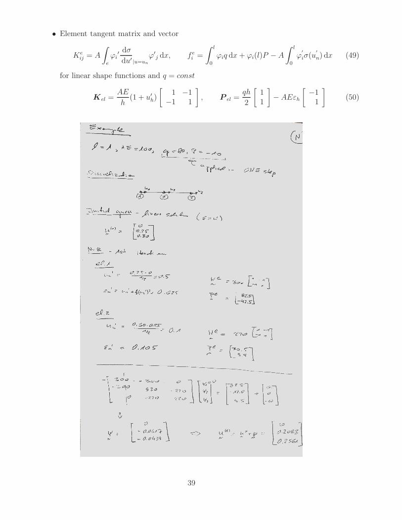
• Element tangent matrix and vector
Keij = A
∫
e
ϕi′ dσ
du′ |u=un
ϕ′j dx, f e
i =
∫ l
0
ϕiq dx+ ϕi(l)P −A∫ l
0
ϕ′
iσ(u′
n) dx (49)
for linear shape functions and q = const
Kel =AE
h(1 + u′h)
[
1 −1−1 1
]
, P el =qh
2
[
11
]
− AEεh[
−11
]
(50)
39

• Results for AE = 100, l = 1, q = 30, P = −10
0 0.2 0.4 0.6 0.8 10
0.01
0.02
0.03
0.04
0.05
0.06
0.07
0 2 4 6 8 100
0.005
0.01
0.015
0.02
0.025
0.03
0.035
0.04
0.045
0.05
Figure 6: 20 finite elements. Displacement along the axis and u(l) versus load level for nonlinear (inred) and linear (in green) models. Maksimum strain is equal to about 20%.
7. Elastic - plastic deformations
• Strong formulation in 1D (t - pseudo time)
−Adσdx
= q(x) ∀x ∈ (0, l), ∀tσ = E(ε− εp) ∀x ∈ (0, l), ∀tε = du
dx∀x ∈ (0, l), ∀t
εp = εp0 ∀x ∈ (0, l), t = 0
u(0) = 0 ∀tAσ(l)n(l) = P ∀t
(51)
• Associated flow rule
εp = γ∂Φ
∂σ(52)
Φ(σ, εp) = |σ −Hεp| − σY 6 0 - Huber-Mises-Hencky (von Mises) yield surface
Φ 6 0, γ > 0, γΦ = 0 - Kuhn-Tucker loading-unloading conditions
σ = ET ε ET = E or ET = EHE+H
• Weak formulationFind u(x) ∈ H1, such that u(0) = 0 and
A
∫ l
0
v′σ(u) dx =
∫ l
0
vq dx+ v(l)P ∀v ∈ V0 (53)
• Newton-Raphson linearizationGiven unk , ε
p(n+1) = εp(n), find ψ(x) ∈ H1, such that ψ(0) = 0 and
A
∫ l
0
v′ET (u(n+1)k )ψ′ dx =
∫ l
0
vq dx+ v(l)P − A∫ l
0
v′σ(n+1)k+1 dx ∀v ∈ V0 (54)
then uk+1 = uk + ψ
40

41

42

43

• Radial return for every Gauss point
σtr = E(εn − εpn +∆ε), If Φ(σtr) > 0 then ∆γ = Φ(σtr)E+H
• Results for a composite bar (two materials)
0 100 200 300 400 5000
1
2
3
4
5
6
7
8x 10
−4
Figure 7: Displacement versus load. Comparison of analytical and numerical solutions.
• Homework
– Perform one step of the Newton-Rahpson method for problem (48).
– For a given εp in a bar compute displacements and stresses using 2 finite elements.
10 Selected other computer methods
1. XFEM - extended FEM
• A FEM version for modeling discontinuities by enrichment of selected shape functions bythe Heaviside function. This way, also theoretically predicted solution behavior is builtinto the approximation (e.g. in vicinity of 2D crack tip by
√r sin( θ
2),√r cos( θ
2), . . .).
• Example of enrichment of selected shape function, let’s say ϕI
uh = . . .+ uIϕI + . . . →uh = . . .+ (uI + aIΨa + bIΨb)ϕI + . . .
(55)
where ΨaϕI ,ΨbϕI are additional shape functions attributed to the same node as the ϕI
function and aI , bI are the corresponding additional degrees of freedom at that node.
• 1D example
2. BEM - boundary element methodLet’s consider the following 2D model problem
−k∆u = f(x, y) in Ωu = u on ∂Ωu
ku = q on ∂Ωq
(56)
• Somigliana’s identity
cu(ξ) =
∫
∂Ω
[u∗(x, ξ)t(x)− t∗(x, ξ)u(x)] dγ +∫
Ω
u∗(x, ξ)f(x) dΩ (57)
where
v∗ = − 1
4πklnr2, t∗ = − 1
2π
(x1 − ξ1)n1 + (x2 − ξ2)n2
r2, r2 = (x1 − ξ1)2 + (x2 − ξ2)2
(58)
44

0 0.2 0.4 0.6 0.8 10
0.5
1
0 0.2 0.4 0.6 0.8 10
0.2
0.4
0 0.2 0.4 0.6 0.8 10
0.5
1
Figure 8: A 1D basis shape function (ϕI) and its two enrichments (ΨaϕI ,ΨbϕI) by distance froma=0.75 and Heaviside function, i.e. Ψa = |x− 0.75|, Ψb = H(x− 0.75).
• Boundary integral equation (for u|∂Ω = 0)
∫
∂Ω
u∗(x, ξ)t(x) dγ +
∫
Ω
u∗(x, ξ)f(x) dΩ = 0 (59)
• Discretization for t ∈ L2(∂Ω) by piecewise constant function and the collocation methodresult in the following SLAE
tj
∫
∂γj
u∗(x, ξi) dγx = −∫
Ω
u∗(x, ξi)f(x) dΩx ∀i, j = 1, 2, . . . , N (60)
• HomeworkUsing the Somigliana identity compute solution to Laplace problem (56) in the center ofa circle of radius R = 3, if f = −4, u = 9, q = 6, k = 1.
3. Meshless, FDM - finite difference method
• MLS (moving least squares) approximation - ϕ(z)
- for a given data set of points S = (x1, y1), . . . (xm, ym)- select a point z
- assume (local) approximation in the formLXY (x) = α1 + α2(x− z) + . . .+ αm(x− z)m−1
- assume weights for residuum, eg. wi =1
(xi − z)2 + ε
- minimize the square of residuum weighted norm ||r||2 = rTWr
with respect to a = [α1, α2, . . . , αm]
- by solution of the following SLAE ATWAa = ATWy
where A is the Vandermonde matrix, A = A(z),W =W (z),a = a(z)
- ϕ(z) = LXY (z) = α1, note: dϕdz6= dLXY
dx |x=z
• A basis function constructed by MLS approximation for the 3rd out of 6 nodes
45

0 1 2 3 4 5 6 7−0.2
0
0.2
0.4
0.6
0.8
1
1.2
Figure 9: A 1D basis function constructed by MLS technique.
Homework
1. Dla zadania (1) i obszaru tam przyjetego (punkt 3).
• Napisac wzory na rozwiazanie MES, jego gradient oraz skladowa strumienia qn wzdluzodcinka AD wiedzac, ze α3 = 2, α4 = −2/3.• sprawdz dokladnosc spelnienie warunku Neumanna jezeli t1 = −1, t2 = 0, t3 = 1− x
2. Dla zadania 1DFind u(x) ∈ H1([a, b]), such that u(a) = u(b) = 0 and
∫ b
a
v′AEu′ dx =
∫ b
a
vq0(l − x) dx ∀v ∈ V0, q0 ∈ R, l = b− a (61)
• Oblicz macierz i wektor dla elementu [2,3] z hierarchiiczna funkcja ksztaltu stopnia 2.
• Napsz wzory na aproksymacje przemieszczen i sily osiowej
• Oblicz reakcje stosujac 1 taki element.
3. Stosujac 2 elementy skonczone z liniowymi fukcjami ksztaltu dla preta
• oblicz czestosci drgan wlasnych i ich postacie
• sprawdz ich ortogonalnosc
4. Zadania nieliniowe
• Wykonaj 1 krok metody Newton-Rahpson dla zadania (48).
• Znajac εp w precie oblicz przemieszczenia, odksztalcenia (calkowite ε) i naprezenia.
46