1

Peter Fox

GIS for Science

ERTH 4750 (98271)

Week 5, Tuesday, February 21, 2012

Introduction to geostatistics. Interpolation techniques

continued (regression, trend surfaces, Thiesses polygons,

splines)

Contents• Reading review

• Assignment 1

• Geostatistics

• Interpolation techniques continued

• Lab on Friday

• Next week2

Reading review for last week

• Chapter 13: Putting your Data on a Map

• Chapter 9: … Thematic maps and Grid surface maps

• Sampling theorem

3

Geostatistics• Geostatistics are a class of statistics applied

to quantities that are distributed geographically.

• There are very specific applications as well as the usual ones.

• As is commonly done, we want to be able to describe our observations in terms of their statistical properties.

4

Geostatistics• In certain GIS applications, we might

want to divide our measurements into a finite number of regions (polygons) within which the measurement has a limited variation.

• We can consider these regions as enclosing homogeneous units.

• The degree to which the points within the region are the same will be decided on a statistical basis.

5

Georegions

6

For example, these regions have been determined based on the values of the measurements (or other attributes) at individual points. The regions may be distinguished simply by the range of measurements, as we do with MapInfo. On the other hand the data may be grouped by its statistical properties. The blue region may have a very different statistical distribution than the red regions, for example.

Sidebar: querying your data• Often to determine georegions for your

statistics you will need to actually LOOK at your data, or subsets of it.– E.g. select countries in Africa with populations

over 2 million and 50 million GDP (gross domestic product)

• We’ll dig into this in future classes but for now see Chapter 8 in MapInfo User Guide: Selecting and Querying Data

• The reality is that we are looking at distributions of our data (sampled…) so … 7

Gaussian Distributions

8

Statistics• We will most often use a Gaussian

distribution (aka normal distribution, or bell-curve) to describe the statistical properties of a group of measurements.

• The variation in the measurements taken over a finite spatial region may be caused by intrinsic spatial variation in the measurement, by uncertainties in the measuring method or equipment, by operator error, ...

9

Mean and standard deviation• The mean, m, of n values of the

measurement of a property z (the average).– m = [ SUM {i=1,n} zi ] / n

• The standard deviation s of the measurements is an indication of the amount of spread in the measurements with respect to the mean.– s2 = [ SUM {i=1,n} ( zi - m )2 ] /n

• The quantity s2 is known as the variance of the measurements.

10

Width of distribution• If the data are truly distributed in a Gaussian

fashion, 65% of all the measurements fall within one s of the mean: i.e. the condition

– s - m < z < s + m

• is true about 2/3 of the time.

• Accordingly, the more spread the measurements are away from the mean, the larger s will be. 11

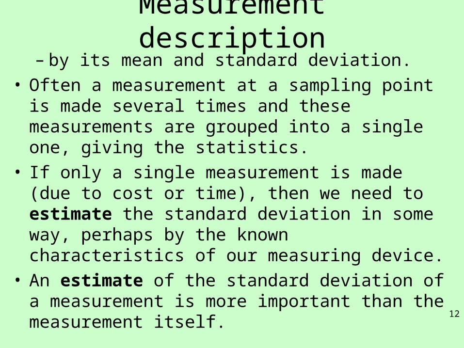
Measurement description– by its mean and standard deviation.

• Often a measurement at a sampling point is made several times and these measurements are grouped into a single one, giving the statistics.

• If only a single measurement is made (due to cost or time), then we need to estimate the standard deviation in some way, perhaps by the known characteristics of our measuring device.

• An estimate of the standard deviation of a measurement is more important than the measurement itself.

12

Weighting• As we discussed briefly last week, the data

are often weighted by the inverse of the variance ( w = s-2 ) when used in modeling or interpolations. In this way, we place more confidence in the better-determined values.

• In classifying the data into groups, we can do so according to either the mean or the scatter or both.

• Excel has the built-in functions AVERAGE and STDEV to calculate the mean and standard deviation for a group of values. 13

More on interpolation

14

Global/ Local Methods• Global methods ~ in which all the known data

are considered

• Local methods ~ in which only nearby data are used.

• Local methods and most often the global methods also rely on the premise that nearby points are more similar than distant points.

• Inverse Distance Weighting (IDW) is an example of a global method.

15

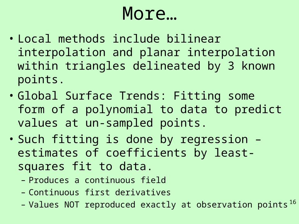
More…• Local methods include bilinear interpolation

and planar interpolation within triangles delineated by 3 known points.

• Global Surface Trends: Fitting some form of a polynomial to data to predict values at un-sampled points.

• Such fitting is done by regression – estimates of coefficients by least-squares fit to data.– Produces a continuous field– Continuous first derivatives– Values NOT reproduced exactly at observation points 16

Geospatial means x and y• In two spatial dimensions (map view x-y

coordinates) the polynomials take the form:

– f(x, y) = SUM r+s <= p ( brs xr ys )

• where b represents a series of coefficients and p is the order of the polynomial trend surface.

• The summation is over all possible positive integers r and s such that their sum is less than or equal to the polynomial order p.

17

p=1 / p=2• For example, if p =1, then

– f(x, y) = b00 + b10 x + b01 y

– which is the equation of a plane.

• If p = 2, then– f(x, y) = b00 + b10 x + b01 y + b11 x y + b20 x2 + b02 y2

• For a polynomial order p the number of coefficients is (p+1)(p+2)/2. In trend

analysis or smoothing, these polynomials are estimated by regression. 18

Regression• Is the process of finding the coefficients that

produce the best-fit to the observed values.

• Best-fit is generally described as minimizing the squares of the misfits at each point, that is, – SUM {i=1,n} [ fi(x, y) – zi(x, y) ]2

• i.e. it is minimized by the choice of coefficients (this minimization is commonly called least-squares).

19

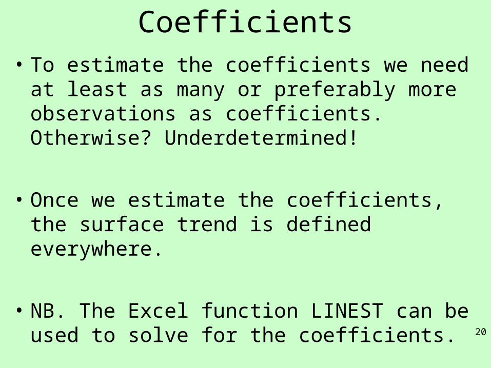
Coefficients• To estimate the coefficients we need at least

as many or preferably more observations as coefficients. Otherwise? Underdetermined!

• Once we estimate the coefficients, the surface trend is defined everywhere.

• NB. The Excel function LINEST can be used to solve for the coefficients.

20

Choices…• The choice of how many coefficients to use

(the order of the polynomial) depends on how smooth you think the variations in the property is, and on how well the data are fit by lower order polynomials.

• In general, adding coefficients always improves the fit to the data to the extreme that if the number of coefficients equals the number of observations, the data can be fit perfectly.

• But this assumes that the data are perfect. 21

Multi-variate analysis• Multivariate analysis is the procedure to use if

we want to see if there is a correlation between any pair of attributes in our data.

• As earlier, you perform a linear regression to find the correlations.

22

Example – gis/data/MULTIVARIATE.xls

23

Multivariate analysis is the procedure to use if we want to see if there is a correlation between any pair of attributes in our data. As earlier, we will perform a linear regression to find the correlations.

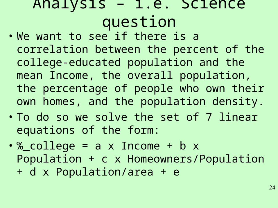
Analysis – i.e. Science question

• We want to see if there is a correlation between the percent of the college-educated population and the mean Income, the overall population, the percentage of people who own their own homes, and the population density.

• To do so we solve the set of 7 linear equations of the form:

• %_college = a x Income + b x Population + c x Homeowners/Population + d x Population/area + e 24

• We solve for for the coefficients a through e.

• This is done with Excel with the LINEST function, giving the result:

– Revealing that population density correlates with college-educated percentage at a significant level.

– => college-educated people prefer to live in densely populated cities.

25

Bi-linear Interpolation• In two-dimensions we can interpolate

between points in a regular or nearly regular grid.

• This interpolation is between 4 points, and hence it is a local method.

– Produces a continuous field– Discontinuous first derivative– Values reproduced exactly at grid points

26

Example

27

• The red squares represent 4 known values of z(x, y) and our goal is to estimate the value of z at the new point (blue circle) at (x0, y0).

t = [ x0 – x1 ] / [ x2 - x1 ] and u = [ y0 – y1 ] / [ y4 - y1 ]

x0,y0

Calculating…• Let

• t = [ x0 – x1 ] / [ x2 - x1 ] and

• u = [ y0 – y1 ] / [ y4 - y1 ]

i.e. the fractional distances the new point is along the grid axes in x and y, respectively, where the subscripts refer to the known points as numbered above.

Then

• z (x0 , y0 ) = (1-t) (1-u) z1 + t (1-u) z2 + t u z3 + (1-t ) u z4

28

Bilinear interpolation for a central point

29

Bilinear interpolation of 4 unequal corner points.

30Lines connecting grid points are straight but diagonals are curved.Bilinear interpolation -> a curvature of the surface within the grid.

Other interpolation• Delaunay triangles: sampled points are

vertices of triangles within which values form a plane.

• Thiessen (Dirichlet / Voronoi) polygons: value at unknown location equals value at nearest known point.

• Splines: piece-wise polynomials estimated using a few local points, go through all known points.

31

More …• Bicubic interpolation

– Requires knowing z (x, y) and slopes dz/dx, dz/dy, d2z/dxdy at all grid points.

• Points and derivatives reproduced exactly at grid points

• Continuous first derivative

• Bicubic spline– Similar to bicubic interpolation but splines are

used to get derivatives at grid points.

• Do some reading on these… will be important for future assignments.

32

Summary• Topics for GIS (for Science)

– Interpolation– (related to) Sampling

• For learning purposes remember:– Demonstrate proficiency in using geospatial applications and tools

(commercial and open-source).

– Present verbally relational analysis and interpretation of a variety of spatial data on maps.

– Demonstrate skill in applying database concepts to build and manipulate a spatial database, SQL, spatial queries, and integration of graphic and tabular data.

– Demonstrate intermediate knowledge of geospatial analysis methods and their applications.

33

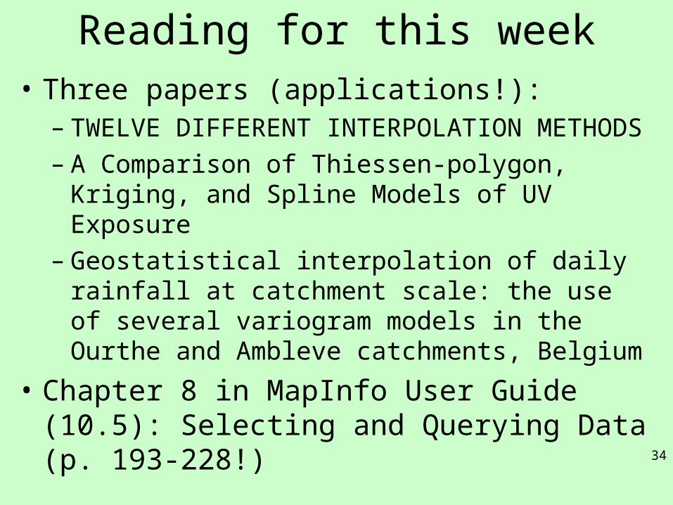
Reading for this week• Three papers (applications!):

– TWELVE DIFFERENT INTERPOLATION METHODS

– A Comparison of Thiessen-polygon, Kriging, and Spline Models of UV Exposure

– Geostatistical interpolation of daily rainfall at catchment scale: the use of several variogram models in the Ourthe and Ambleve catchments, Belgium

• Chapter 8 in MapInfo User Guide (10.5): Selecting and Querying Data (p. 193-228!)

34

Friday Feb. 24th• Lab session – with a walk through of

examples first– Interpolation

• Plus, continuation of MapInfo examples– Thematic maps

35

Next classes

• Interpolation continued (variograms, kriging)

• Definition of term projects

• Lab on Friday (2nd)

36

MapInfo master:

thematic maps

while U wait