1 sample space and probability - athena scientific
TRANSCRIPT
1
Sample Space and
Probability
Contents
1.1. Sets . . . . . . . . . . . . . . . . . . . . . . . . . . . p. 31.2. Probabilistic Models . . . . . . . . . . . . . . . . . . . . p. 61.3. Conditional Probability . . . . . . . . . . . . . . . . . p. 181.4. Total Probability Theorem and Bayes’ Rule . . . . . . . . p. 281.5. Independence . . . . . . . . . . . . . . . . . . . . . . p. 341.6. Counting . . . . . . . . . . . . . . . . . . . . . . . p. 441.7. Summary and Discussion . . . . . . . . . . . . . . . . p. 51
Problems . . . . . . . . . . . . . . . . . . . . . . . . p. 53
1
2 Sample Space and Probability Chap. 1
“Probability” is a very useful concept, but can be interpreted in a number ofways. As an illustration, consider the following.
A patient is admitted to the hospital and a potentially life-saving drug isadministered. The following dialog takes place between the nurse and aconcerned relative.
RELATIVE: Nurse, what is the probability that the drug will work?NURSE: I hope it works, we’ll know tomorrow.RELATIVE: Yes, but what is the probability that it will?NURSE: Each case is different, we have to wait.RELATIVE: But let’s see, out of a hundred patients that are treated undersimilar conditions, how many times would you expect it to work?NURSE (somewhat annoyed): I told you, every person is different, for someit works, for some it doesn’t.RELATIVE (insisting): Then tell me, if you had to bet whether it will workor not, which side of the bet would you take?NURSE (cheering up for a moment): I’d bet it will work.RELATIVE (somewhat relieved): OK, now, would you be willing to lose twodollars if it doesn’t work, and gain one dollar if it does?NURSE (exasperated): What a sick thought! You are wasting my time!
In this conversation, the relative attempts to use the concept of probabilityto discuss an uncertain situation. The nurse’s initial response indicates that themeaning of “probability” is not uniformly shared or understood, and the relativetries to make it more concrete. The first approach is to define probability interms of frequency of occurrence, as a percentage of successes in a moderatelylarge number of similar situations. Such an interpretation is often natural. Forexample, when we say that a perfectly manufactured coin lands on heads “withprobability 50%,” we typically mean “roughly half of the time.” But the nursemay not be entirely wrong in refusing to discuss in such terms. What if thiswas an experimental drug that was administered for the very first time in thishospital or in the nurse’s experience?
While there are many situations involving uncertainty in which the fre-quency interpretation is appropriate, there are other situations in which it isnot. Consider, for example, a scholar who asserts that the Iliad and the Odysseywere composed by the same person, with probability 90%. Such an assertionconveys some information, but not in terms of frequencies, since the subject isa one-time event. Rather, it is an expression of the scholar’s subjective be-lief. One might think that subjective beliefs are not interesting, at least from amathematical or scientific point of view. On the other hand, people often haveto make choices in the presence of uncertainty, and a systematic way of makinguse of their beliefs is a prerequisite for successful, or at least consistent, decisionmaking.
Sec. 1.1 Sets 3
In fact, the choices and actions of a rational person, can reveal a lot aboutthe inner-held subjective probabilities, even if the person does not make conscioususe of probabilistic reasoning. Indeed, the last part of the earlier dialog was anattempt to infer the nurse’s beliefs in an indirect manner. Since the nurse waswilling to accept a one-for-one bet that the drug would work, we may inferthat the probability of success was judged to be at least 50%. And had thenurse accepted the last proposed bet (two-for-one), that would have indicated asuccess probability of at least 2/3.
Rather than dwelling further into philosophical issues about the appropri-ateness of probabilistic reasoning, we will simply take it as a given that the theoryof probability is useful in a broad variety of contexts, including some where theassumed probabilities only reflect subjective beliefs. There is a large body ofsuccessful applications in science, engineering, medicine, management, etc., andon the basis of this empirical evidence, probability theory is an extremely usefultool.
Our main objective in this book is to develop the art of describing un-certainty in terms of probabilistic models, as well as the skill of probabilisticreasoning. The first step, which is the subject of this chapter, is to describethe generic structure of such models, and their basic properties. The models weconsider assign probabilities to collections (sets) of possible outcomes. For thisreason, we must begin with a short review of set theory.
1.1 SETS
Probability makes extensive use of set operations, so let us introduce at theoutset the relevant notation and terminology.
A set is a collection of objects, which are the elements of the set. If S isa set and x is an element of S, we write x ∈ S. If x is not an element of S, wewrite x /∈ S. A set can have no elements, in which case it is called the emptyset, denoted by Ø.
Sets can be specified in a variety of ways. If S contains a finite number ofelements, say x1, x2, . . . , xn, we write it as a list of the elements, in braces:
S = {x1, x2, . . . , xn}.
For example, the set of possible outcomes of a die roll is {1, 2, 3, 4, 5, 6}, and theset of possible outcomes of a coin toss is {H, T}, where H stands for “heads”and T stands for “tails.”
If S contains infinitely many elements x1, x2, . . ., which can be enumeratedin a list (so that there are as many elements as there are positive integers) wewrite
S = {x1, x2, . . .},and we say that S is countably infinite. For example, the set of even integerscan be written as {0, 2,−2, 4,−4, . . .}, and is countably infinite.
4 Sample Space and Probability Chap. 1
Alternatively, we can consider the set of all x that have a certain propertyP , and denote it by
{x |x satisfies P}.
(The symbol “|” is to be read as “such that.”) For example, the set of evenintegers can be written as {k | k/2 is integer}. Similarly, the set of all scalars xin the interval [0, 1] can be written as {x | 0 ≤ x ≤ 1}. Note that the elements xof the latter set take a continuous range of values, and cannot be written downin a list (a proof is sketched in the end-of-chapter problems); such a set is saidto be uncountable.
If every element of a set S is also an element of a set T , we say that Sis a subset of T , and we write S ⊂ T or T ⊃ S. If S ⊂ T and T ⊂ S, thetwo sets are equal, and we write S = T . It is also expedient to introduce auniversal set, denoted by Ω, which contains all objects that could conceivablybe of interest in a particular context. Having specified the context in terms of auniversal set Ω, we only consider sets S that are subsets of Ω.
Set Operations
The complement of a set S, with respect to the universe Ω, is the set {x ∈Ω |x /∈ S} of all elements of Ω that do not belong to S, and is denoted by Sc.Note that Ωc = Ø.
The union of two sets S and T is the set of all elements that belong to Sor T (or both), and is denoted by S ∪ T . The intersection of two sets S and Tis the set of all elements that belong to both S and T , and is denoted by S ∩ T .Thus,
S ∪ T = {x |x ∈ S or x ∈ T},
andS ∩ T = {x |x ∈ S and x ∈ T}.
In some cases, we will have to consider the union or the intersection of several,even infinitely many sets, defined in the obvious way. For example, if for everypositive integer n, we are given a set Sn, then
∞⋃n=1
Sn = S1 ∪ S2 ∪ · · · = {x |x ∈ Sn for some n},
and ∞⋂n=1
Sn = S1 ∩ S2 ∩ · · · = {x |x ∈ Sn for all n}.
Two sets are said to be disjoint if their intersection is empty. More generally,several sets are said to be disjoint if no two of them have a common element. Acollection of sets is said to be a partition of a set S if the sets in the collectionare disjoint and their union is S.

Sec. 1.1 Sets 5
If x and y are two objects, we use (x, y) to denote the ordered pair of xand y. The set of scalars (real numbers) is denoted by �; the set of pairs (ortriplets) of scalars, i.e., the two-dimensional plane (or three-dimensional space,respectively) is denoted by �2 (or �3, respectively).
Sets and the associated operations are easy to visualize in terms of Venndiagrams, as illustrated in Fig. 1.1.
S
T
Ω
T
Ω Ω
S S
T
(a) (b)
S
T
Ω
(c)
S
T
Ω
(d) (e)
U S
TΩ
(f )
U
Figure 1.2: Examples of Venn diagrams. (a) The shaded region is S ∩ T . (b)The shaded region is S ∪ T . (c) The shaded region is S ∩ T c. (d) Here, T ⊂ S.The shaded region is the complement of S. (e) The sets S, T , and U are disjoint.(f) The sets S, T , and U form a partition of the set Ω.
The Algebra of Sets
Set operations have several properties, which are elementary consequences of thedefinitions. Some examples are:
S ∪ T = T ∪ S, S ∪ (T ∪ U) = (S ∪ T ) ∪ U,S ∩ (T ∪ U) = (S ∩ T ) ∪ (S ∩ U), S ∪ (T ∩ U) = (S ∪ T ) ∩ (S ∪ U),
(Sc)c = S, S ∩ Sc = Ø,S ∪ Ω = Ω, S ∩ Ω = S.
Two particularly useful properties are given by De Morgan’s laws whichstate that (⋃
n
Sn
)c
=⋂n
Scn,
(⋂n
Sn
)c
=⋃n
Scn.
To establish the first law, suppose that x ∈ (∪nSn)c. Then, x /∈ ∪nSn, whichimplies that for every n, we have x /∈ Sn. Thus, x belongs to the complement
6 Sample Space and Probability Chap. 1
of every Sn, and x ∈ ∩nScn. This shows that (∪nSn)c ⊂ ∩nSc
n. The converseinclusion is established by reversing the above argument, and the first law follows.The argument for the second law is similar.
1.2 PROBABILISTIC MODELS
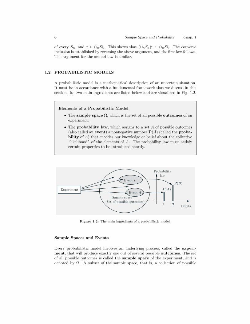
A probabilistic model is a mathematical description of an uncertain situation.It must be in accordance with a fundamental framework that we discuss in thissection. Its two main ingredients are listed below and are visualized in Fig. 1.2.
Elements of a Probabilistic Model
• The sample space Ω, which is the set of all possible outcomes of anexperiment.
• The probability law, which assigns to a set A of possible outcomes(also called an event) a nonnegative number P(A) (called the proba-bility of A) that encodes our knowledge or belief about the collective“likelihood” of the elements of A. The probability law must satisfycertain properties to be introduced shortly.
Experiment
Sample space(Set of possible outcomes)
Event A
Event B
A BEvents
P(A)
P(B)
Probabilitylaw
Figure 1.2: The main ingredients of a probabilistic model.
Sample Spaces and Events
Every probabilistic model involves an underlying process, called the experi-ment, that will produce exactly one out of several possible outcomes. The setof all possible outcomes is called the sample space of the experiment, and isdenoted by Ω. A subset of the sample space, that is, a collection of possible
Sec. 1.2 Probabilistic Models 7
outcomes, is called an event.† There is no restriction on what constitutes anexperiment. For example, it could be a single toss of a coin, or three tosses,or an infinite sequence of tosses. However, it is important to note that in ourformulation of a probabilistic model, there is only one experiment. So, threetosses of a coin constitute a single experiment, rather than three experiments.
The sample space of an experiment may consist of a finite or an infinitenumber of possible outcomes. Finite sample spaces are conceptually and math-ematically simpler. Still, sample spaces with an infinite number of elements arequite common. For an example, consider throwing a dart on a square target andviewing the point of impact as the outcome.
Choosing an Appropriate Sample Space
Regardless of their number, different elements of the sample space should bedistinct and mutually exclusive so that when the experiment is carried out,there is a unique outcome. For example, the sample space associated with theroll of a die cannot contain “1 or 3” as a possible outcome and also “1 or 4”as another possible outcome, because we would not be able to assign a uniqueoutcome when the roll is a 1.
A given physical situation may be modeled in several different ways, de-pending on the kind of questions that we are interested in. Generally, the samplespace chosen for a probabilistic model must be collectively exhaustive, in thesense that no matter what happens in the experiment, we always obtain an out-come that has been included in the sample space. In addition, the sample spaceshould have enough detail to distinguish between all outcomes of interest to themodeler, while avoiding irrelevant details.
Example 1.1. Consider two alternative games, both involving ten successive cointosses:
Game 1: We receive $1 each time a head comes up.
Game 2: We receive $1 for every coin toss, up to and including the first timea head comes up. Then, we receive $2 for every coin toss, up to the secondtime a head comes up. More generally, the dollar amount per toss is doubledeach time a head comes up.
† Any collection of possible outcomes, including the entire sample space Ω andits complement, the empty set Ø, may qualify as an event. Strictly speaking, however,some sets have to be excluded. In particular, when dealing with probabilistic modelsinvolving an uncountably infinite sample space, there are certain unusual subsets forwhich one cannot associate meaningful probabilities. This is an intricate technical issue,involving the mathematics of measure theory. Fortunately, such pathological subsetsdo not arise in the problems considered in this text or in practice, and the issue can besafely ignored.
8 Sample Space and Probability Chap. 1
In game 1, it is only the total number of heads in the ten-toss sequence that mat-ters, while in game 2, the order of heads and tails is also important. Thus, ina probabilistic model for game 1, we can work with a sample space consisting ofeleven possible outcomes, namely, 0, 1, . . . , 10. In game 2, a finer grain descriptionof the experiment is called for, and it is more appropriate to let the sample spaceconsist of every possible ten-long sequence of heads and tails.
Sequential Models
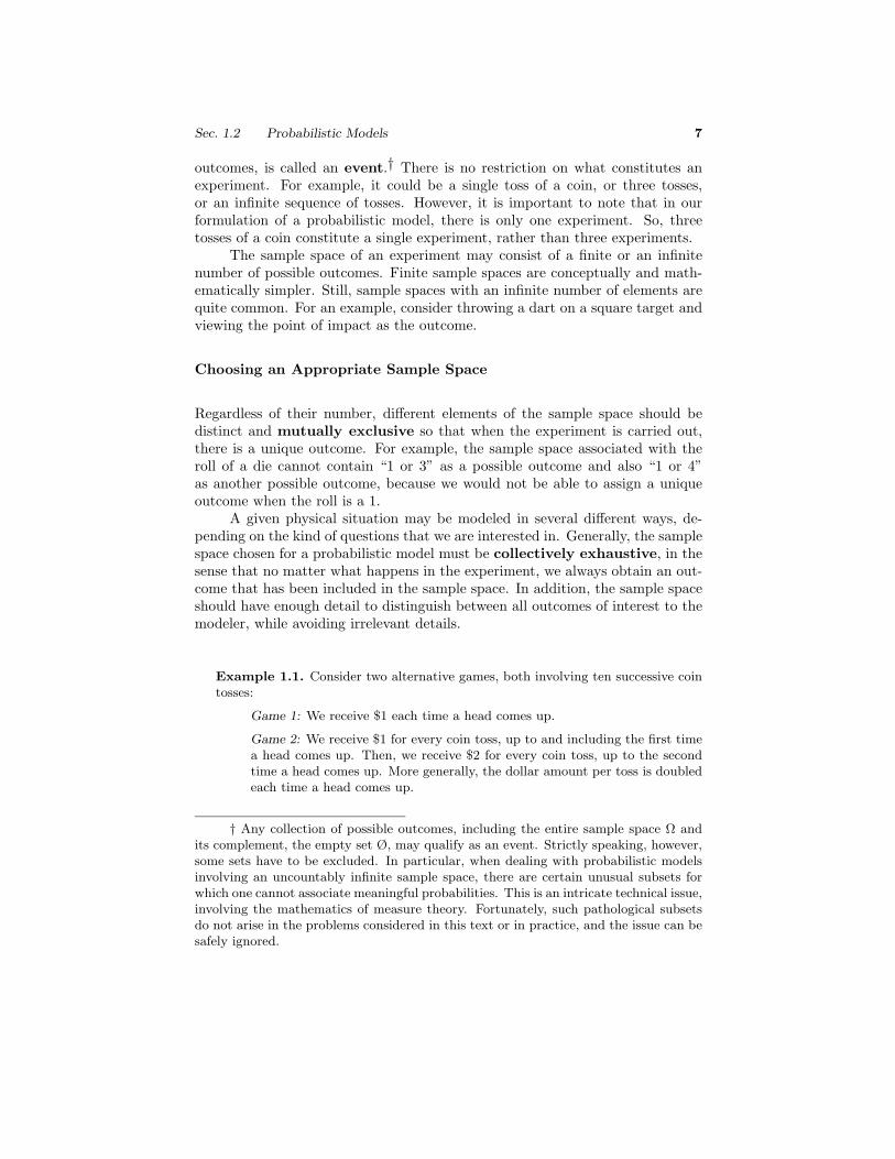
Many experiments have an inherently sequential character, such as for exampletossing a coin three times, or observing the value of a stock on five successivedays, or receiving eight successive digits at a communication receiver. It is thenoften useful to describe the experiment and the associated sample space by meansof a tree-based sequential description, as in Fig. 1.3.
11 2
2
3
3
4
4
Tree-based sequentialdescription
Sample space for a pair of rolls
1st roll
2nd roll
1,11,21,31,4
1
2
3
4
Root
Leaves
Figure 1.3: Two equivalent descriptions of the sample space of an experimentinvolving two rolls of a 4-sided die. The possible outcomes are all the ordered pairsof the form (i, j), where i is the result of the first roll, and j is the result of thesecond. These outcomes can be arranged in a 2-dimensional grid as in the figureon the left, or they can be described by the tree on the right, which reflects thesequential character of the experiment. Here, each possible outcome correspondsto a leaf of the tree and is associated with the unique path from the root tothat leaf. The shaded area on the left is the event {(1, 4), (2, 4), (3, 4), (4, 4)}that the result of the second roll is 4. That same event can be described by theset of leaves highlighted on the right. Note also that every node of the tree canbe identified with an event, namely, the set of all leaves downstream from thatnode. For example, the node labeled by a 1 can be identified with the event{(1, 1), (1, 2), (1, 3), (1, 4)} that the result of the first roll is 1.
Probability Laws
Suppose we have settled on the sample space Ω associated with an experiment.Then, to complete the probabilistic model, we must introduce a probability
Sec. 1.2 Probabilistic Models 9
law. Intuitively, this specifies the “likelihood” of any outcome, or of any set ofpossible outcomes (an event, as we have called it earlier). More precisely, theprobability law assigns to every event A, a number P(A), called the probabilityof A, satisfying the following axioms.
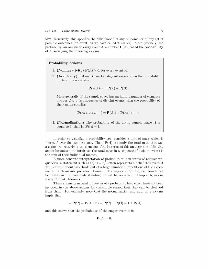
Probability Axioms
1. (Nonnegativity) P(A) ≥ 0, for every event A.
2. (Additivity) If A and B are two disjoint events, then the probabilityof their union satisfies
P(A ∪ B) = P(A) + P(B).
More generally, if the sample space has an infinite number of elementsand A1, A2, . . . is a sequence of disjoint events, then the probability oftheir union satisfies
P(A1 ∪ A2 ∪ · · ·) = P(A1) + P(A2) + · · · .
3. (Normalization) The probability of the entire sample space Ω isequal to 1, that is, P(Ω) = 1.
In order to visualize a probability law, consider a unit of mass which is“spread” over the sample space. Then, P(A) is simply the total mass that wasassigned collectively to the elements of A. In terms of this analogy, the additivityaxiom becomes quite intuitive: the total mass in a sequence of disjoint events isthe sum of their individual masses.
A more concrete interpretation of probabilities is in terms of relative fre-quencies: a statement such as P(A) = 2/3 often represents a belief that event Awill occur in about two thirds out of a large number of repetitions of the exper-iment. Such an interpretation, though not always appropriate, can sometimesfacilitate our intuitive understanding. It will be revisited in Chapter 5, in ourstudy of limit theorems.
There are many natural properties of a probability law, which have not beenincluded in the above axioms for the simple reason that they can be derivedfrom them. For example, note that the normalization and additivity axiomsimply that
1 = P(Ω) = P(Ω ∪ Ø) = P(Ω) + P(Ø) = 1 + P(Ø),
and this shows that the probability of the empty event is 0:
P(Ø) = 0.
10 Sample Space and Probability Chap. 1
As another example, consider three disjoint events A1, A2, and A3. We can usethe additivity axiom for two disjoint events repeatedly, to obtain
P(A1 ∪ A2 ∪ A3) = P(A1 ∪ (A2 ∪ A3)
)= P(A1) + P(A2 ∪ A3)= P(A1) + P(A2) + P(A3).
Proceeding similarly, we obtain that the probability of the union of finitely manydisjoint events is always equal to the sum of the probabilities of these events.More such properties will be considered shortly.
Discrete Models
Here is an illustration of how to construct a probability law starting from somecommon sense assumptions about a model.
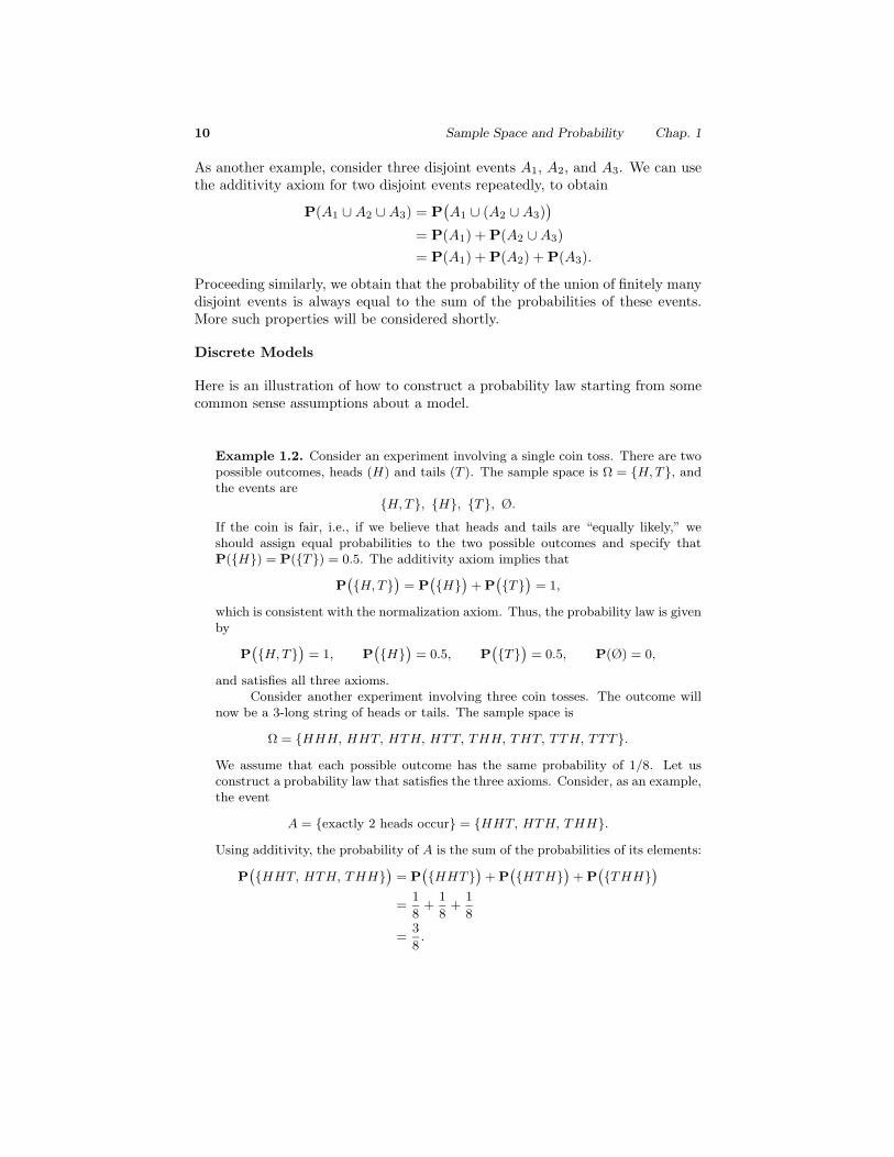
Example 1.2. Consider an experiment involving a single coin toss. There are twopossible outcomes, heads (H) and tails (T ). The sample space is Ω = {H, T}, andthe events are
{H, T}, {H}, {T}, Ø.
If the coin is fair, i.e., if we believe that heads and tails are “equally likely,” weshould assign equal probabilities to the two possible outcomes and specify thatP({H}) = P({T}) = 0.5. The additivity axiom implies that
P({H, T}
)= P
({H}
)+ P
({T}
)= 1,
which is consistent with the normalization axiom. Thus, the probability law is givenby
P({H, T}
)= 1, P
({H}
)= 0.5, P
({T}
)= 0.5, P(Ø) = 0,
and satisfies all three axioms.Consider another experiment involving three coin tosses. The outcome will
now be a 3-long string of heads or tails. The sample space is
Ω = {HHH, HHT, HTH, HTT, THH, THT, TTH, TTT}.
We assume that each possible outcome has the same probability of 1/8. Let usconstruct a probability law that satisfies the three axioms. Consider, as an example,the event
A = {exactly 2 heads occur} = {HHT, HTH, THH}.
Using additivity, the probability of A is the sum of the probabilities of its elements:
P({HHT, HTH, THH}
)= P
({HHT}
)+ P
({HTH}
)+ P
({THH}
)=
1
8+
1
8+
1
8
=3
8.
Sec. 1.2 Probabilistic Models 11
Similarly, the probability of any event is equal to 1/8 times the number of possibleoutcomes contained in the event. This defines a probability law that satisfies thethree axioms.
By using the additivity axiom and by generalizing the reasoning in thepreceding example, we reach the following conclusion.
Discrete Probability Law
If the sample space consists of a finite number of possible outcomes, then theprobability law is specified by the probabilities of the events that consist ofa single element. In particular, the probability of any event {s1, s2, . . . , sn}is the sum of the probabilities of its elements:
P({s1, s2, . . . , sn}
)= P(s1) + P(s2) + · · · + P(sn).
Note that we are using here the simpler notation P(si) to denote the prob-ability of the event {si}, instead of the more precise P({si}). This conventionwill be used throughout the remainder of the book.
In the special case where the probabilities P(s1), . . . ,P(sn) are all the same(by necessity equal to 1/n, in view of the normalization axiom), we obtain thefollowing.
Discrete Uniform Probability Law
If the sample space consists of n possible outcomes which are equally likely(i.e., all single-element events have the same probability), then the proba-bility of any event A is given by
P(A) =number of elements of A
n.
Let us provide a few more examples of sample spaces and probability laws.
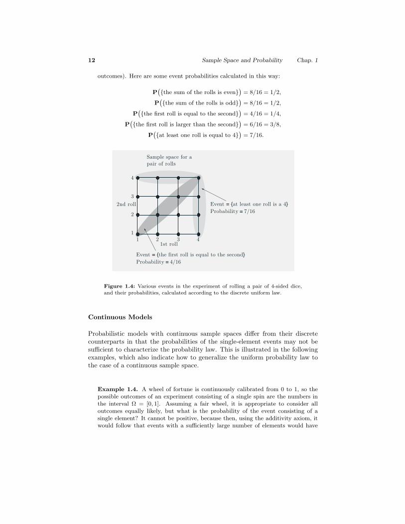
Example 1.3. Consider the experiment of rolling a pair of 4-sided dice (cf. Fig.1.4). We assume the dice are fair, and we interpret this assumption to mean thateach of the sixteen possible outcomes [pairs (i, j), with i, j = 1, 2, 3, 4], has the sameprobability of 1/16. To calculate the probability of an event, we must count thenumber of elements of the event and divide by 16 (the total number of possible
12 Sample Space and Probability Chap. 1
outcomes). Here are some event probabilities calculated in this way:
P({the sum of the rolls is even}
)= 8/16 = 1/2,
P({the sum of the rolls is odd}
)= 8/16 = 1/2,
P({the first roll is equal to the second}
)= 4/16 = 1/4,
P({the first roll is larger than the second}
)= 6/16 = 3/8,
P({at least one roll is equal to 4}
)= 7/16.
11 2
2
3
3
4
4
Sample space for apair of rolls
1st roll
2nd roll
Event = {the first roll is equal to the second}Probability = 4/16
Event = {at least one roll is a 4}Probability = 7/16
Figure 1.4: Various events in the experiment of rolling a pair of 4-sided dice,and their probabilities, calculated according to the discrete uniform law.
Continuous Models
Probabilistic models with continuous sample spaces differ from their discretecounterparts in that the probabilities of the single-element events may not besufficient to characterize the probability law. This is illustrated in the followingexamples, which also indicate how to generalize the uniform probability law tothe case of a continuous sample space.
Example 1.4. A wheel of fortune is continuously calibrated from 0 to 1, so thepossible outcomes of an experiment consisting of a single spin are the numbers inthe interval Ω = [0, 1]. Assuming a fair wheel, it is appropriate to consider alloutcomes equally likely, but what is the probability of the event consisting of asingle element? It cannot be positive, because then, using the additivity axiom, itwould follow that events with a sufficiently large number of elements would have
Sec. 1.2 Probabilistic Models 13
probability larger than 1. Therefore, the probability of any event that consists of asingle element must be 0.
In this example, it makes sense to assign probability b − a to any subinter-val [a, b] of [0, 1], and to calculate the probability of a more complicated set by
evaluating its “length.”† This assignment satisfies the three probability axioms andqualifies as a legitimate probability law.
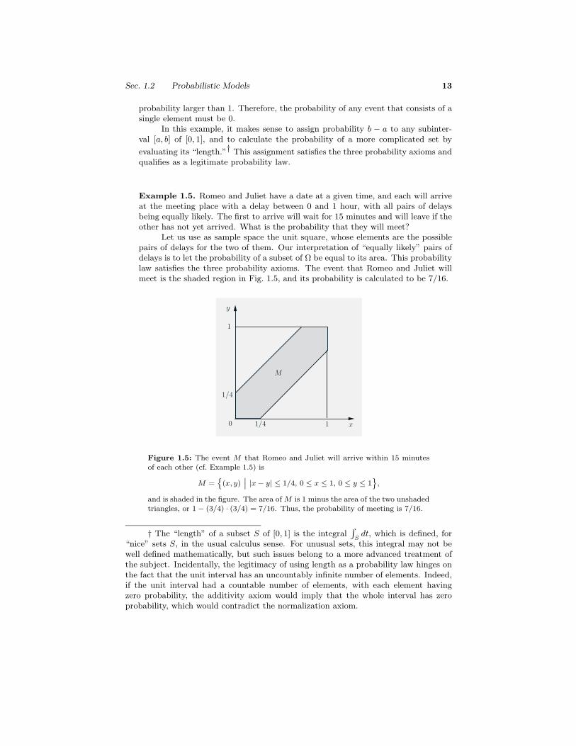
Example 1.5. Romeo and Juliet have a date at a given time, and each will arriveat the meeting place with a delay between 0 and 1 hour, with all pairs of delaysbeing equally likely. The first to arrive will wait for 15 minutes and will leave if theother has not yet arrived. What is the probability that they will meet?
Let us use as sample space the unit square, whose elements are the possiblepairs of delays for the two of them. Our interpretation of “equally likely” pairs ofdelays is to let the probability of a subset of Ω be equal to its area. This probabilitylaw satisfies the three probability axioms. The event that Romeo and Juliet willmeet is the shaded region in Fig. 1.5, and its probability is calculated to be 7/16.
0 1
1
1/4
1/4 x
y
M
Figure 1.5: The event M that Romeo and Juliet will arrive within 15 minutesof each other (cf. Example 1.5) is
M ={
(x, y)∣∣ |x − y| ≤ 1/4, 0 ≤ x ≤ 1, 0 ≤ y ≤ 1
},
and is shaded in the figure. The area of M is 1 minus the area of the two unshadedtriangles, or 1 − (3/4) · (3/4) = 7/16. Thus, the probability of meeting is 7/16.
† The “length” of a subset S of [0, 1] is the integral∫
Sdt, which is defined, for
“nice” sets S, in the usual calculus sense. For unusual sets, this integral may not bewell defined mathematically, but such issues belong to a more advanced treatment ofthe subject. Incidentally, the legitimacy of using length as a probability law hinges onthe fact that the unit interval has an uncountably infinite number of elements. Indeed,if the unit interval had a countable number of elements, with each element havingzero probability, the additivity axiom would imply that the whole interval has zeroprobability, which would contradict the normalization axiom.
14 Sample Space and Probability Chap. 1
Properties of Probability Laws
Probability laws have a number of properties, which can be deduced from theaxioms. Some of them are summarized below.
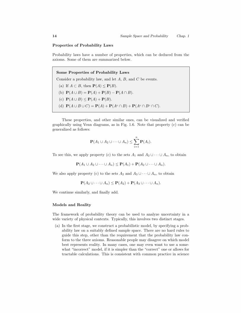
Some Properties of Probability Laws
Consider a probability law, and let A, B, and C be events.
(a) If A ⊂ B, then P(A) ≤ P(B).
(b) P(A ∪ B) = P(A) + P(B) − P(A ∩ B).
(c) P(A ∪ B) ≤ P(A) + P(B).
(d) P(A ∪ B ∪ C) = P(A) + P(Ac ∩ B) + P(Ac ∩ Bc ∩ C).
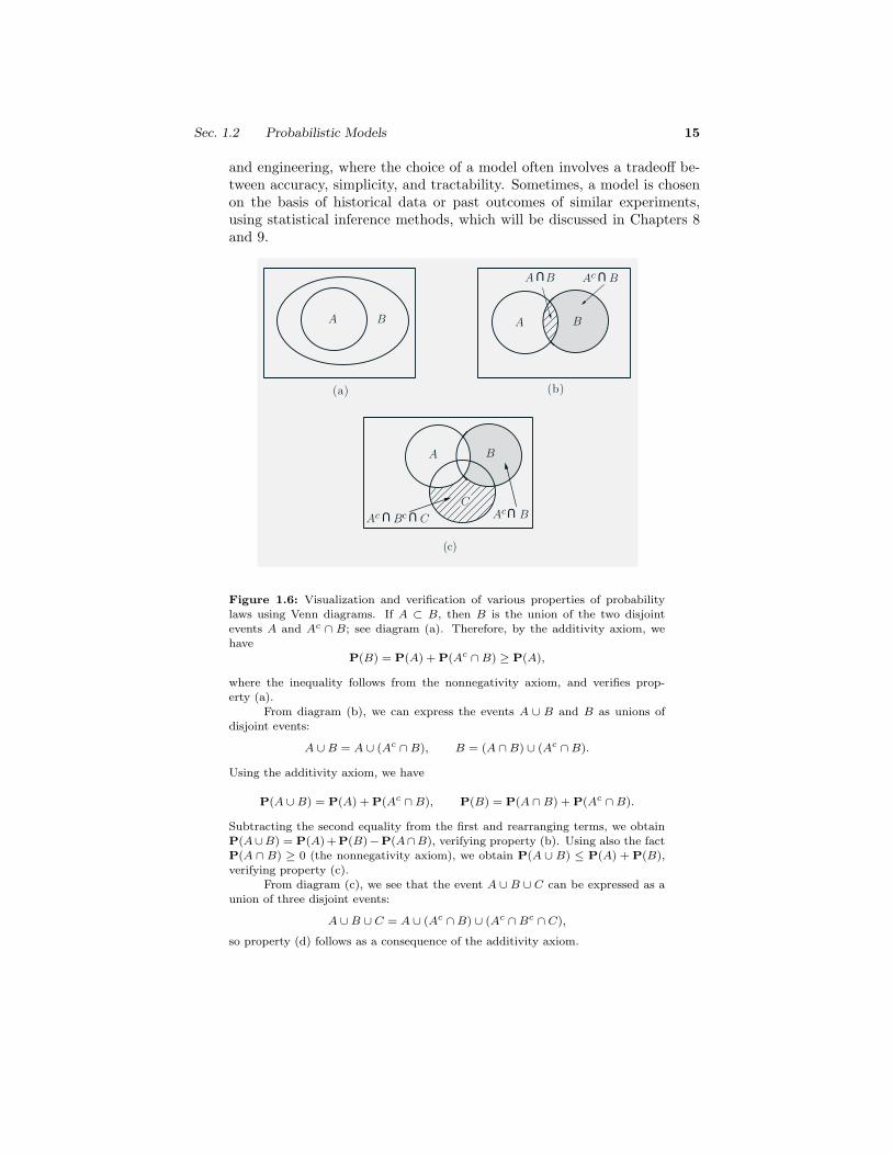
These properties, and other similar ones, can be visualized and verifiedgraphically using Venn diagrams, as in Fig. 1.6. Note that property (c) can begeneralized as follows:
P(A1 ∪ A2 ∪ · · · ∪ An) ≤n∑
i=1
P(Ai).
To see this, we apply property (c) to the sets A1 and A2 ∪ · · · ∪ An, to obtain
P(A1 ∪ A2 ∪ · · · ∪ An) ≤ P(A1) + P(A2 ∪ · · · ∪ An).
We also apply property (c) to the sets A2 and A3 ∪ · · · ∪ An, to obtain
P(A2 ∪ · · · ∪ An) ≤ P(A2) + P(A3 ∪ · · · ∪ An).
We continue similarly, and finally add.
Models and Reality
The framework of probability theory can be used to analyze uncertainty in awide variety of physical contexts. Typically, this involves two distinct stages.
(a) In the first stage, we construct a probabilistic model, by specifying a prob-ability law on a suitably defined sample space. There are no hard rules toguide this step, other than the requirement that the probability law con-form to the three axioms. Reasonable people may disagree on which modelbest represents reality. In many cases, one may even want to use a some-what “incorrect” model, if it is simpler than the “correct” one or allows fortractable calculations. This is consistent with common practice in science
Sec. 1.2 Probabilistic Models 15
and engineering, where the choice of a model often involves a tradeoff be-tween accuracy, simplicity, and tractability. Sometimes, a model is chosenon the basis of historical data or past outcomes of similar experiments,using statistical inference methods, which will be discussed in Chapters 8and 9.
BcAc
A B
(a)
(c)
A B
CB
U
AcU U
C
(b)
A B
B
U
A B
U
Ac
Figure 1.6: Visualization and verification of various properties of probabilitylaws using Venn diagrams. If A ⊂ B, then B is the union of the two disjointevents A and Ac ∩ B; see diagram (a). Therefore, by the additivity axiom, wehave
P(B) = P(A) + P(Ac ∩ B) ≥ P(A),
where the inequality follows from the nonnegativity axiom, and verifies prop-erty (a).
From diagram (b), we can express the events A ∪ B and B as unions ofdisjoint events:
A ∪ B = A ∪ (Ac ∩ B), B = (A ∩ B) ∪ (Ac ∩ B).
Using the additivity axiom, we have
P(A ∪ B) = P(A) + P(Ac ∩ B), P(B) = P(A ∩ B) + P(Ac ∩ B).
Subtracting the second equality from the first and rearranging terms, we obtainP(A∪B) = P(A)+P(B)−P(A∩B), verifying property (b). Using also the factP(A ∩ B) ≥ 0 (the nonnegativity axiom), we obtain P(A ∪ B) ≤ P(A) + P(B),verifying property (c).
From diagram (c), we see that the event A ∪ B ∪ C can be expressed as aunion of three disjoint events:
A ∪ B ∪ C = A ∪ (Ac ∩ B) ∪ (Ac ∩ Bc ∩ C),
so property (d) follows as a consequence of the additivity axiom.

16 Sample Space and Probability Chap. 1
(b) In the second stage, we work within a fully specified probabilistic model andderive the probabilities of certain events, or deduce some interesting prop-erties. While the first stage entails the often open-ended task of connectingthe real world with mathematics, the second one is tightly regulated by therules of ordinary logic and the axioms of probability. Difficulties may arisein the latter if some required calculations are complex, or if a probabilitylaw is specified in an indirect fashion. Even so, there is no room for ambi-guity: all conceivable questions have precise answers and it is only a matterof developing the skill to arrive at them.
Probability theory is full of “paradoxes” in which different calculationmethods seem to give different answers to the same question. Invariably though,these apparent inconsistencies turn out to reflect poorly specified or ambiguousprobabilistic models. An example, Bertrand’s paradox, is shown in Fig. 1.7.
.
.
A
.B
C
midpoint of ABchord through C
(a)
at angle Φchord
V
Φ
(b)
Figure 1.7: This example, presented by L. F. Bertrand in 1889, illustrates theneed to specify unambiguously a probabilistic model. Consider a circle and anequilateral triangle inscribed in the circle. What is the probability that the lengthof a randomly chosen chord of the circle is greater than the side of the triangle?The answer here depends on the precise meaning of “randomly chosen.” The twomethods illustrated in parts (a) and (b) of the figure lead to contradictory results.
In (a), we take a radius of the circle, such as AB, and we choose a pointC on that radius, with all points being equally likely. We then draw the chordthrough C that is orthogonal to AB. From elementary geometry, AB intersectsthe triangle at the midpoint of AB, so the probability that the length of the chordis greater than the side is 1/2.
In (b), we take a point on the circle, such as the vertex V , we draw thetangent to the circle through V , and we draw a line through V that forms a randomangle Φ with the tangent, with all angles being equally likely. We consider thechord obtained by the intersection of this line with the circle. From elementarygeometry, the length of the chord is greater than the side of the triangle if Φ isbetween π/3 and 2π/3. Since Φ takes values between 0 and π, the probabilitythat the length of the chord is greater than the side is 1/3.
Sec. 1.2 Probabilistic Models 17
A Brief History of Probability
• B.C.E. Games of chance were popular in ancient Greece and Rome, butno scientific development of the subject took place, possibly because thenumber system used by the Greeks did not facilitate algebraic calculations.The development of probability based on sound scientific analysis had toawait the development of the modern arithmetic system by the Hindus andthe Arabs in the second half of the first millennium, as well as the flood ofscientific ideas generated by the Renaissance.
• 16th century. Girolamo Cardano, a colorful and controversial Italianmathematician, publishes the first book describing correct methods for cal-culating probabilities in games of chance involving dice and cards.
• 17th century. A correspondence between Fermat and Pascal touches uponseveral interesting probability questions, and motivates further study in thefield.
• 18th century. Jacob Bernoulli studies repeated coin tossing and introducesthe first law of large numbers, which lays a foundation for linking theoreti-cal probability concepts and empirical fact. Several mathematicians, such asDaniel Bernoulli, Leibnitz, Bayes, and Lagrange, make important contribu-tions to probability theory and its use in analyzing real-world phenomena.De Moivre introduces the normal distribution and proves the first form ofthe central limit theorem.
• 19th century. Laplace publishes an influential book that establishes theimportance of probability as a quantitative field and contains many originalcontributions, including a more general version of the central limit theo-rem. Legendre and Gauss apply probability to astronomical predictions,using the method of least squares, thus pointing the way to a vast range ofapplications. Poisson publishes an influential book with many original con-tributions, including the Poisson distribution. Chebyshev, and his studentsMarkov and Lyapunov, study limit theorems and raise the standards ofmathematical rigor in the field. Throughout this period, probability theoryis largely viewed as a natural science, its primary goal being the explanationof physical phenomena. Consistently with this goal, probabilities are mainlyinterpreted as limits of relative frequencies in the context of repeatable ex-periments.
• 20th century. Relative frequency is abandoned as the conceptual foun-dation of probability theory in favor of a now universally used axiomaticsystem, introduced by Kolmogorov. Similar to other branches of mathe-matics, the development of probability theory from the axioms relies onlyon logical correctness, regardless of its relevance to physical phenomena.Nonetheless, probability theory is used pervasively in science and engineer-ing because of its ability to describe and interpret most types of uncertainphenomena in the real world.
18 Sample Space and Probability Chap. 1
1.3 CONDITIONAL PROBABILITY
Conditional probability provides us with a way to reason about the outcomeof an experiment, based on partial information. Here are some examples ofsituations we have in mind:
(a) In an experiment involving two successive rolls of a die, you are told thatthe sum of the two rolls is 9. How likely is it that the first roll was a 6?
(b) In a word guessing game, the first letter of the word is a “t”. What is thelikelihood that the second letter is an “h”?
(c) How likely is it that a person has a certain disease given that a medicaltest was negative?
(d) A spot shows up on a radar screen. How likely is it to correspond to anaircraft?
In more precise terms, given an experiment, a corresponding sample space,and a probability law, suppose that we know that the outcome is within somegiven event B. We wish to quantify the likelihood that the outcome also belongsto some other given event A. We thus seek to construct a new probability law,which takes into account the available knowledge: a probability law that forany event A, specifies the conditional probability of A given B, denoted byP(A |B).
We would like the conditional probabilities P(A |B) of different events Ato constitute a legitimate probability law, which satisfies the probability axioms.The conditional probabilities should also be consistent with our intuition in im-portant special cases, e.g., when all possible outcomes of the experiment areequally likely. For example, suppose that all six possible outcomes of a fair dieroll are equally likely. If we are told that the outcome is even, we are left withonly three possible outcomes, namely, 2, 4, and 6. These three outcomes wereequally likely to start with, and so they should remain equally likely given theadditional knowledge that the outcome was even. Thus, it is reasonable to let
P(the outcome is 6 | the outcome is even) =13.
This argument suggests that an appropriate definition of conditional probabilitywhen all outcomes are equally likely, is given by
P(A |B) =number of elements of A ∩ B
number of elements of B.
Generalizing the argument, we introduce the following definition of condi-tional probability:
P(A |B) =P(A ∩ B)
P(B),
Sec. 1.3 Conditional Probability 19
where we assume that P(B) > 0; the conditional probability is undefined if theconditioning event has zero probability. In words, out of the total probability ofthe elements of B, P(A |B) is the fraction that is assigned to possible outcomesthat also belong to A.
Conditional Probabilities Specify a Probability Law
For a fixed event B, it can be verified that the conditional probabilities P(A |B)form a legitimate probability law that satisfies the three axioms. Indeed, non-negativity is clear. Furthermore,
P(Ω |B) =P(Ω ∩ B)
P(B)=
P(B)P(B)
= 1,
and the normalization axiom is also satisfied. To verify the additivity axiom, wewrite for any two disjoint events A1 and A2,
P(A1 ∪ A2 |B) =P
((A1 ∪ A2) ∩ B
)P(B)
=P((A1 ∩ B) ∪ (A2 ∩ B))
P(B)
=P(A1 ∩ B) + P(A2 ∩ B)
P(B)
=P(A1 ∩ B)
P(B)+
P(A2 ∩ B)P(B)
= P(A1 |B) + P(A2 |B),
where for the third equality, we used the fact that A1 ∩ B and A2 ∩ B aredisjoint sets, and the additivity axiom for the (unconditional) probability law.The argument for a countable collection of disjoint sets is similar.
Since conditional probabilities constitute a legitimate probability law, allgeneral properties of probability laws remain valid. For example, a fact such asP(A ∪ C) ≤ P(A) + P(C) translates to the new fact
P(A ∪ C |B) ≤ P(A |B) + P(C |B).
Let us also note that since we have P(B |B) = P(B)/P(B) = 1, all of the con-ditional probability is concentrated on B. Thus, we might as well discard allpossible outcomes outside B and treat the conditional probabilities as a proba-bility law defined on the new universe B.
Let us summarize the conclusions reached so far.
20 Sample Space and Probability Chap. 1
Properties of Conditional Probability
• The conditional probability of an event A, given an event B withP(B) > 0, is defined by
P(A |B) =P(A ∩ B)
P(B),
and specifies a new (conditional) probability law on the same samplespace Ω. In particular, all properties of probability laws remain validfor conditional probability laws.
• Conditional probabilities can also be viewed as a probability law on anew universe B, because all of the conditional probability is concen-trated on B.
• If the possible outcomes are finitely many and equally likely, then
P(A |B) =number of elements of A ∩ B
number of elements of B.
Example 1.6. We toss a fair coin three successive times. We wish to find theconditional probability P(A |B) when A and B are the events
A = {more heads than tails come up}, B = {1st toss is a head}.
The sample space consists of eight sequences,
Ω = {HHH, HHT, HTH, HTT, THH, THT, TTH, TTT},
which we assume to be equally likely. The event B consists of the four elementsHHH, HHT, HTH, HTT , so its probability is
P(B) =4
8.
The event A ∩ B consists of the three elements HHH, HHT, HTH, so its proba-bility is
P(A ∩ B) =3
8.
Thus, the conditional probability P(A |B) is
P(A |B) =P(A ∩ B)
P(B)=
3/8
4/8=
3
4.
Because all possible outcomes are equally likely here, we can also compute P(A |B)using a shortcut. We can bypass the calculation of P(B) and P(A∩B), and simply

Sec. 1.3 Conditional Probability 21
divide the number of elements shared by A and B (which is 3) with the number ofelements of B (which is 4), to obtain the same result 3/4.
Example 1.7. A fair 4-sided die is rolled twice and we assume that all sixteenpossible outcomes are equally likely. Let X and Y be the result of the 1st and the2nd roll, respectively. We wish to determine the conditional probability P(A |B),where
A ={max(X, Y ) = m
}, B =
{min(X, Y ) = 2
},
and m takes each of the values 1, 2, 3, 4.As in the preceding example, we can first determine the probabilities P(A∩B)
and P(B) by counting the number of elements of A ∩ B and B, respectively, anddividing by 16. Alternatively, we can directly divide the number of elements ofA ∩ B with the number of elements of B; see Fig. 1.8.
11 2
2
3
3
4
4
All outcomes equally likely
Probability = 1/16
1st roll X
2nd roll Y
B
Figure 1.8: Sample space of an experiment involving two rolls of a 4-sided die.(cf. Example 1.7). The conditioning event B = {min(X, Y ) = 2} consists of the5-element shaded set. The set A = {max(X, Y ) = m} shares with B two elementsif m = 3 or m = 4, one element if m = 2, and no element if m = 1. Thus, we have
P({max(X, Y ) = m}
∣∣ B)
=
{2/5, if m = 3 or m = 4,
1/5, if m = 2,
0, if m = 1.
Example 1.8. A conservative design team, call it C, and an innovative designteam, call it N, are asked to separately design a new product within a month. Frompast experience we know that:
(a) The probability that team C is successful is 2/3.
(b) The probability that team N is successful is 1/2.
(c) The probability that at least one team is successful is 3/4.
22 Sample Space and Probability Chap. 1
Assuming that exactly one successful design is produced, what is the probabilitythat it was designed by team N?
There are four possible outcomes here, corresponding to the four combinationsof success and failure of the two teams:
SS: both succeed, FF : both fail,SF : C succeeds, N fails, FS: C fails, N succeeds.
We were given that the probabilities of these outcomes satisfy
P(SS) + P(SF ) =2
3, P(SS) + P(FS) =
1
2, P(SS) + P(SF ) + P(FS) =
3
4.
From these relations, together with the normalization equation
P(SS) + P(SF ) + P(FS) + P(FF ) = 1,
we can obtain the probabilities of individual outcomes:
P(SS) =5
12, P(SF ) =
1
4, P(FS) =
1
12, P(FF ) =
1
4.
The desired conditional probability is
P(FS
∣∣ {SF, FS})
=
1
121
4+
1
12
=1
4.
Using Conditional Probability for Modeling
When constructing probabilistic models for experiments that have a sequentialcharacter, it is often natural and convenient to first specify conditional prob-abilities and then use them to determine unconditional probabilities. The ruleP(A∩B) = P(B)P(A |B), which is a restatement of the definition of conditionalprobability, is often helpful in this process.
Example 1.9. Radar Detection. If an aircraft is present in a certain area, aradar detects it and generates an alarm signal with probability 0.99. If an aircraft isnot present, the radar generates a (false) alarm, with probability 0.10. We assumethat an aircraft is present with probability 0.05. What is the probability of noaircraft presence and a false alarm? What is the probability of aircraft presenceand no detection?
A sequential representation of the experiment is appropriate here, as shownin Fig. 1.9. Let A and B be the events
A = {an aircraft is present},B = {the radar generates an alarm},
Sec. 1.3 Conditional Probability 23
and consider also their complements
Ac = {an aircraft is not present},Bc = {the radar does not generate an alarm}.
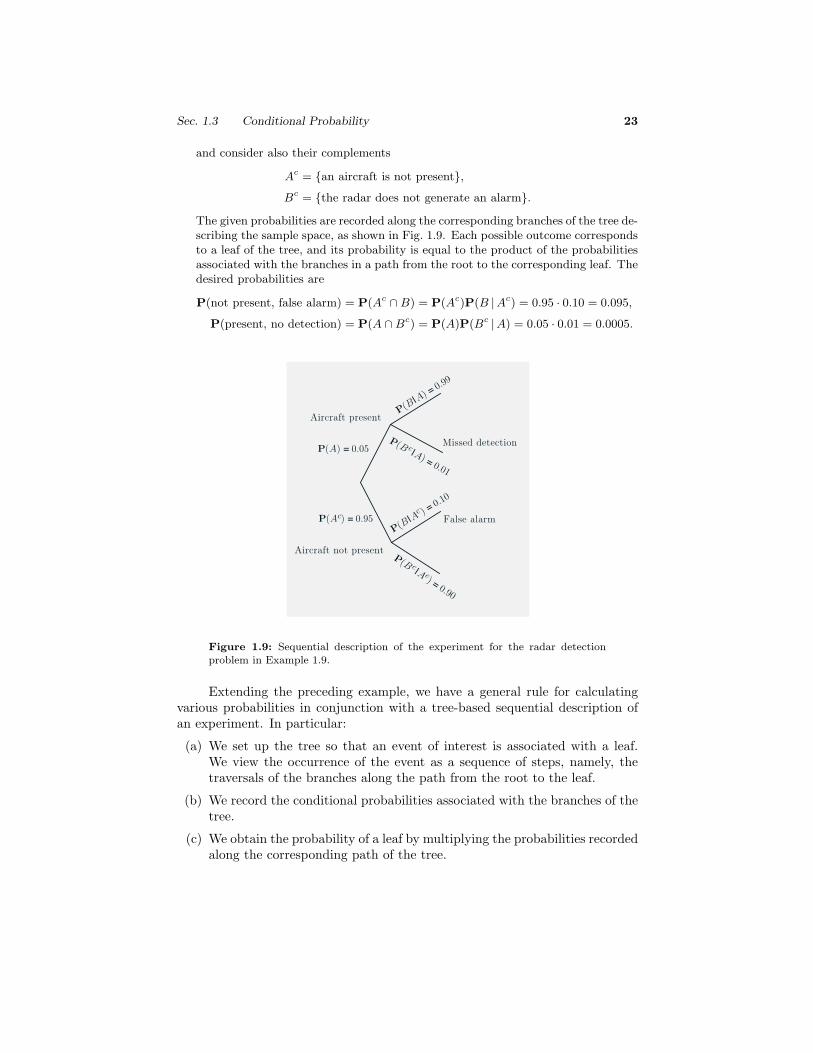
The given probabilities are recorded along the corresponding branches of the tree de-scribing the sample space, as shown in Fig. 1.9. Each possible outcome correspondsto a leaf of the tree, and its probability is equal to the product of the probabilitiesassociated with the branches in a path from the root to the corresponding leaf. Thedesired probabilities are
P(not present, false alarm) = P(Ac ∩ B) = P(Ac)P(B |Ac) = 0.95 · 0.10 = 0.095,
P(present, no detection) = P(A ∩ Bc) = P(A)P(Bc |A) = 0.05 · 0.01 = 0.0005.
P(B| A) =
0.99
P(A) = 0.05P(B c| A) = 0.01
P(B| A
c ) = 0.1
0
P(B c| A c) = 0.90
False alarm
Missed detection
Aircraft present
Aircraft not present
P(Ac) = 0.95
Figure 1.9: Sequential description of the experiment for the radar detectionproblem in Example 1.9.
Extending the preceding example, we have a general rule for calculatingvarious probabilities in conjunction with a tree-based sequential description ofan experiment. In particular:
(a) We set up the tree so that an event of interest is associated with a leaf.We view the occurrence of the event as a sequence of steps, namely, thetraversals of the branches along the path from the root to the leaf.
(b) We record the conditional probabilities associated with the branches of thetree.
(c) We obtain the probability of a leaf by multiplying the probabilities recordedalong the corresponding path of the tree.

24 Sample Space and Probability Chap. 1
In mathematical terms, we are dealing with an event A which occurs if andonly if each one of several events A1, . . . , An has occurred, i.e., A = A1 ∩ A2 ∩· · · ∩An. The occurrence of A is viewed as an occurrence of A1, followed by theoccurrence of A2, then of A3, etc., and it is visualized as a path with n branches,corresponding to the events A1, . . . , An. The probability of A is given by thefollowing rule (see also Fig. 1.10).
Multiplication Rule
Assuming that all of the conditioning events have positive probability, wehave
P(∩n
i=1 Ai
)= P(A1)P(A2 |A1)P(A3 |A1 ∩ A2) · · ·P
(An | ∩n−1
i=1 Ai
).
The multiplication rule can be verified by writing
P(∩n
i=1 Ai
)= P(A1) ·
P(A1 ∩ A2)P(A1)
· P(A1 ∩ A2 ∩ A3)P(A1 ∩ A2)
· · · P(∩n
i=1 Ai
)P
(∩n−1
i=1 Ai
) ,
. . .P(A1) P(A3 |A1 ∩ A2)P(A2 |A1)
Event A1 ∩ A2 ∩ A3
P(An |A1 ∩ A2 ∩ ∩ An−1)
A1 A2 An−1 AnA3
Event A1 ∩ A2 ∩ ∩ An. . .
. . .
Figure 1.10: Visualization of the multiplication rule. The intersection eventA = A1 ∩ A2 ∩ · · · ∩ An is associated with a particular path on a tree thatdescribes the experiment. We associate the branches of this path with the eventsA1, . . . , An, and we record next to the branches the corresponding conditionalprobabilities.
The final node of the path corresponds to the intersection event A, andits probability is obtained by multiplying the conditional probabilities recordedalong the branches of the path
P(A1 ∩ A2 ∩ · · · ∩ An) = P(A1)P(A2 |A1) · · ·P(An |A1 ∩ A2 ∩ · · · ∩ An−1).
Note that any intermediate node along the path also corresponds to some inter-section event and its probability is obtained by multiplying the correspondingconditional probabilities up to that node. For example, the event A1 ∩ A2 ∩ A3
corresponds to the node shown in the figure, and its probability is
P(A1 ∩ A2 ∩ A3) = P(A1)P(A2 |A1)P(A3 |A1 ∩ A2).
Sec. 1.3 Conditional Probability 25
and by using the definition of conditional probability to rewrite the right-handside above as
P(A1)P(A2 |A1)P(A3 |A1 ∩ A2) · · ·P(An | ∩n−1
i=1 Ai
).
For the case of just two events, A1 and A2, the multiplication rule is simply thedefinition of conditional probability.
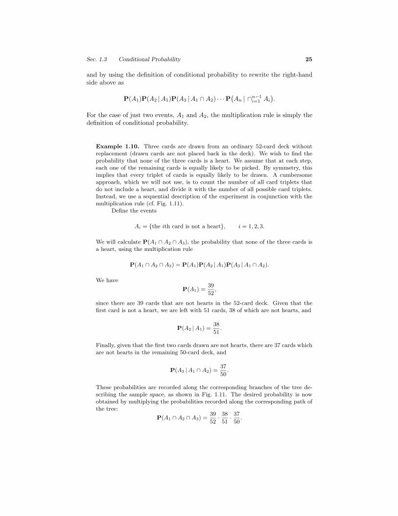
Example 1.10. Three cards are drawn from an ordinary 52-card deck withoutreplacement (drawn cards are not placed back in the deck). We wish to find theprobability that none of the three cards is a heart. We assume that at each step,each one of the remaining cards is equally likely to be picked. By symmetry, thisimplies that every triplet of cards is equally likely to be drawn. A cumbersomeapproach, which we will not use, is to count the number of all card triplets thatdo not include a heart, and divide it with the number of all possible card triplets.Instead, we use a sequential description of the experiment in conjunction with themultiplication rule (cf. Fig. 1.11).
Define the events
Ai = {the ith card is not a heart}, i = 1, 2, 3.
We will calculate P(A1 ∩ A2 ∩ A3), the probability that none of the three cards isa heart, using the multiplication rule
P(A1 ∩ A2 ∩ A3) = P(A1)P(A2 |A1)P(A3 |A1 ∩ A2).
We have
P(A1) =39
52,
since there are 39 cards that are not hearts in the 52-card deck. Given that thefirst card is not a heart, we are left with 51 cards, 38 of which are not hearts, and
P(A2 |A1) =38
51.
Finally, given that the first two cards drawn are not hearts, there are 37 cards whichare not hearts in the remaining 50-card deck, and
P(A3 |A1 ∩ A2) =37
50.
These probabilities are recorded along the corresponding branches of the tree de-scribing the sample space, as shown in Fig. 1.11. The desired probability is nowobtained by multiplying the probabilities recorded along the corresponding path ofthe tree:
P(A1 ∩ A2 ∩ A3) =39
52· 38
51· 37
50.
26 Sample Space and Probability Chap. 1
Not a heart39/52
38/51
37/50
Not a heart
Not a heart
Heart
Heart
Heart
13/52
13/51
13/50 Figure 1.11: Sequential descriptionof the experiment in the 3-card se-lection problem of Example 1.10.
Note that once the probabilities are recorded along the tree, the probabilityof several other events can be similarly calculated. For example,
P(1st is not a heart and 2nd is a heart) =39
52· 13
51,
P(1st and 2nd are not hearts, and 3rd is a heart) =39
52· 38
51· 13
50.
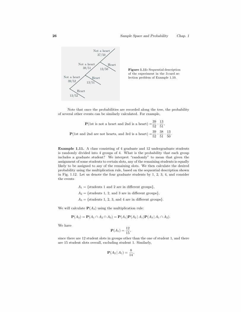
Example 1.11. A class consisting of 4 graduate and 12 undergraduate studentsis randomly divided into 4 groups of 4. What is the probability that each groupincludes a graduate student? We interpret “randomly” to mean that given theassignment of some students to certain slots, any of the remaining students is equallylikely to be assigned to any of the remaining slots. We then calculate the desiredprobability using the multiplication rule, based on the sequential description shownin Fig. 1.12. Let us denote the four graduate students by 1, 2, 3, 4, and considerthe events
A1 = {students 1 and 2 are in different groups},A2 = {students 1, 2, and 3 are in different groups},A3 = {students 1, 2, 3, and 4 are in different groups}.
We will calculate P(A3) using the multiplication rule:
P(A3) = P(A1 ∩ A2 ∩ A3) = P(A1)P(A2 |A1)P(A3 |A1 ∩ A2).
We have
P(A1) =12
15,
since there are 12 student slots in groups other than the one of student 1, and thereare 15 student slots overall, excluding student 1. Similarly,
P(A2 |A1) =8
14,
Sec. 1.3 Conditional Probability 27
Students 1 & 2 arein different groups
12/15
Students 1, 2, & 3 arein different groups
8/14
Students 1, 2, 3, & 4 arein different groups
4/13
Figure 1.12: Sequential descrip-tion of the experiment in the stu-dent problem of Example 1.11.
since there are 8 student slots in groups other than those of students 1 and 2, andthere are 14 student slots, excluding students 1 and 2. Also,
P(A3 |A1 ∩ A2) =4
13,
since there are 4 student slots in groups other than those of students 1, 2, and 3,and there are 13 student slots, excluding students 1, 2, and 3. Thus, the desiredprobability is
12
15· 8
14· 4
13,
and is obtained by multiplying the conditional probabilities along the correspondingpath of the tree in Fig. 1.12.
Example 1.12. The Monty Hall Problem. This is a much discussed puzzle,based on an old American game show. You are told that a prize is equally likely tobe found behind any one of three closed doors in front of you. You point to one ofthe doors. A friend opens for you one of the remaining two doors, after making surethat the prize is not behind it. At this point, you can stick to your initial choice,or switch to the other unopened door. You win the prize if it lies behind your finalchoice of a door. Consider the following strategies:
(a) Stick to your initial choice.
(b) Switch to the other unopened door.
(c) You first point to door 1. If door 2 is opened, you do not switch. If door 3 isopened, you switch.
Which is the best strategy? To answer the question, let us calculate the probabilityof winning under each of the three strategies.
Under the strategy of no switching, your initial choice will determine whetheryou win or not, and the probability of winning is 1/3. This is because the prize isequally likely to be behind each door.
Under the strategy of switching, if the prize is behind the initially chosendoor (probability 1/3), you do not win. If it is not (probability 2/3), and given that

28 Sample Space and Probability Chap. 1
another door without a prize has been opened for you, you will get to the winningdoor once you switch. Thus, the probability of winning is now 2/3, so (b) is a betterstrategy than (a).
Consider now strategy (c). Under this strategy, there is insufficient informa-tion for determining the probability of winning. The answer depends on the waythat your friend chooses which door to open. Let us consider two possibilities.
Suppose that if the prize is behind door 1, your friend always chooses to opendoor 2. (If the prize is behind door 2 or 3, your friend has no choice.) If the prizeis behind door 1, your friend opens door 2, you do not switch, and you win. If theprize is behind door 2, your friend opens door 3, you switch, and you win. If theprize is behind door 3, your friend opens door 2, you do not switch, and you lose.Thus, the probability of winning is 2/3, so strategy (c) in this case is as good asstrategy (b).
Suppose now that if the prize is behind door 1, your friend is equally likely toopen either door 2 or 3. If the prize is behind door 1 (probability 1/3), and if yourfriend opens door 2 (probability 1/2), you do not switch and you win (probability1/6). But if your friend opens door 3, you switch and you lose. If the prize is behinddoor 2, your friend opens door 3, you switch, and you win (probability 1/3). If theprize is behind door 3, your friend opens door 2, you do not switch and you lose.Thus, the probability of winning is 1/6 + 1/3 = 1/2, so strategy (c) in this case isinferior to strategy (b).
1.4 TOTAL PROBABILITY THEOREM AND BAYES’ RULE
In this section, we explore some applications of conditional probability. We startwith the following theorem, which is often useful for computing the probabilitiesof various events, using a “divide-and-conquer” approach.
Total Probability Theorem
Let A1, . . . , An be disjoint events that form a partition of the sample space(each possible outcome is included in exactly one of the events A1, . . . , An)and assume that P(Ai) > 0, for all i. Then, for any event B, we have
P(B) = P(A1 ∩ B) + · · · + P(An ∩ B)= P(A1)P(B |A1) + · · · + P(An)P(B |An).
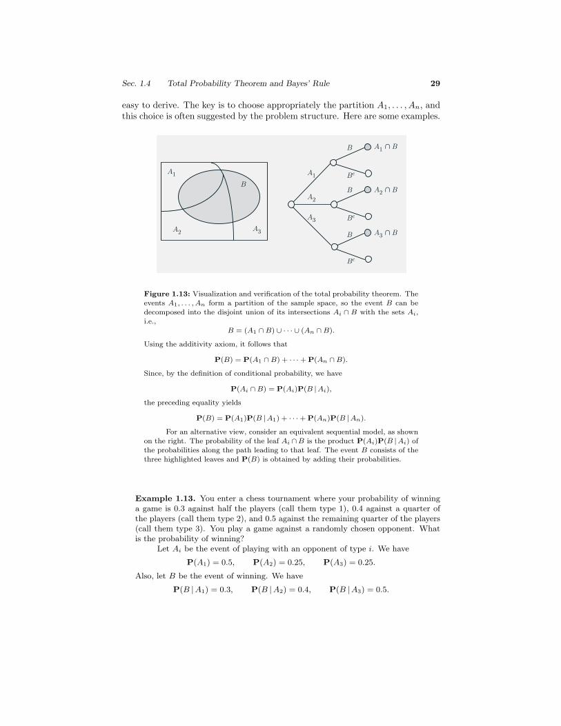
The theorem is visualized and proved in Fig. 1.13. Intuitively, we are par-titioning the sample space into a number of scenarios (events) Ai. Then, theprobability that B occurs is a weighted average of its conditional probabilityunder each scenario, where each scenario is weighted according to its (uncondi-tional) probability. One of the uses of the theorem is to compute the probabilityof various events B for which the conditional probabilities P(B |Ai) are known or
Sec. 1.4 Total Probability Theorem and Bayes’ Rule 29
easy to derive. The key is to choose appropriately the partition A1, . . . , An, andthis choice is often suggested by the problem structure. Here are some examples.
B
A1 ∩ B
A1
A2 A3
B
B
B
Bc
Bc
Bc
A1
A2
A3
A2 ∩ B
A3 ∩ B
Figure 1.13: Visualization and verification of the total probability theorem. Theevents A1, . . . , An form a partition of the sample space, so the event B can bedecomposed into the disjoint union of its intersections Ai ∩ B with the sets Ai,i.e.,
B = (A1 ∩ B) ∪ · · · ∪ (An ∩ B).
Using the additivity axiom, it follows that
P(B) = P(A1 ∩ B) + · · · + P(An ∩ B).
Since, by the definition of conditional probability, we have
P(Ai ∩ B) = P(Ai)P(B |Ai),
the preceding equality yields
P(B) = P(A1)P(B |A1) + · · · + P(An)P(B |An).
For an alternative view, consider an equivalent sequential model, as shownon the right. The probability of the leaf Ai ∩B is the product P(Ai)P(B |Ai) ofthe probabilities along the path leading to that leaf. The event B consists of thethree highlighted leaves and P(B) is obtained by adding their probabilities.
Example 1.13. You enter a chess tournament where your probability of winninga game is 0.3 against half the players (call them type 1), 0.4 against a quarter ofthe players (call them type 2), and 0.5 against the remaining quarter of the players(call them type 3). You play a game against a randomly chosen opponent. Whatis the probability of winning?
Let Ai be the event of playing with an opponent of type i. We have
P(A1) = 0.5, P(A2) = 0.25, P(A3) = 0.25.
Also, let B be the event of winning. We have
P(B |A1) = 0.3, P(B |A2) = 0.4, P(B |A3) = 0.5.
30 Sample Space and Probability Chap. 1
Thus, by the total probability theorem, the probability of winning is
P(B) = P(A1)P(B |A1) + P(A2)P(B |A2) + P(A3)P(B |A3)
= 0.5 · 0.3 + 0.25 · 0.4 + 0.25 · 0.5
= 0.375.
Example 1.14. You roll a fair four-sided die. If the result is 1 or 2, you roll oncemore but otherwise, you stop. What is the probability that the sum total of yourrolls is at least 4?
Let Ai be the event that the result of first roll is i, and note that P(Ai) = 1/4for each i. Let B be the event that the sum total is at least 4. Given the event A1,the sum total will be at least 4 if the second roll results in 3 or 4, which happenswith probability 1/2. Similarly, given the event A2, the sum total will be at least4 if the second roll results in 2, 3, or 4, which happens with probability 3/4. Also,given the event A3, you stop and the sum total remains below 4. Therefore,
P(B |A1) =1
2, P(B |A2) =
3
4, P(B |A3) = 0, P(B |A4) = 1.
By the total probability theorem,
P(B) =1
4· 1
2+
1
4· 3
4+
1
4· 0 +
1
4· 1 =
9
16.
The total probability theorem can be applied repeatedly to calculate proba-bilities in experiments that have a sequential character, as shown in the followingexample.
Example 1.15. Alice is taking a probability class and at the end of each weekshe can be either up-to-date or she may have fallen behind. If she is up-to-date ina given week, the probability that she will be up-to-date (or behind) in the nextweek is 0.8 (or 0.2, respectively). If she is behind in a given week, the probabilitythat she will be up-to-date (or behind) in the next week is 0.4 (or 0.6, respectively).Alice is (by default) up-to-date when she starts the class. What is the probabilitythat she is up-to-date after three weeks?
Let Ui and Bi be the events that Alice is up-to-date or behind, respectively,after i weeks. According to the total probability theorem, the desired probabilityP(U3) is given by
P(U3) = P(U2)P(U3 |U2) + P(B2)P(U3 |B2) = P(U2) · 0.8 + P(B2) · 0.4.
The probabilities P(U2) and P(B2) can also be calculated using the total probabilitytheorem:
P(U2) = P(U1)P(U2 |U1) + P(B1)P(U2 |B1) = P(U1) · 0.8 + P(B1) · 0.4,
P(B2) = P(U1)P(B2 |U1) + P(B1)P(B2 |B1) = P(U1) · 0.2 + P(B1) · 0.6.
Sec. 1.4 Total Probability Theorem and Bayes’ Rule 31
Finally, since Alice starts her class up-to-date, we have
P(U1) = 0.8, P(B1) = 0.2.
We can now combine the preceding three equations to obtain
P(U2) = 0.8 · 0.8 + 0.2 · 0.4 = 0.72,
P(B2) = 0.8 · 0.2 + 0.2 · 0.6 = 0.28,
and by using the above probabilities in the formula for P(U3):
P(U3) = 0.72 · 0.8 + 0.28 · 0.4 = 0.688.
Note that we could have calculated the desired probability P(U3) by con-structing a tree description of the experiment, then calculating the probability ofevery element of U3 using the multiplication rule on the tree, and adding. However,there are cases where the calculation based on the total probability theorem is moreconvenient. For example, suppose we are interested in the probability P(U20) thatAlice is up-to-date after 20 weeks. Calculating this probability using the multipli-cation rule is very cumbersome, because the tree representing the experiment is 20stages deep and has 220 leaves. On the other hand, with a computer, a sequentialcalculation using the total probability formulas
P(Ui+1) = P(Ui) · 0.8 + P(Bi) · 0.4,
P(Bi+1) = P(Ui) · 0.2 + P(Bi) · 0.6,
and the initial conditions P(U1) = 0.8, P(B1) = 0.2, is very simple.
Inference and Bayes’ Rule
The total probability theorem is often used in conjunction with the followingcelebrated theorem, which relates conditional probabilities of the form P(A |B)to conditional probabilities of the form P(B |A), in which the order of the con-ditioning is reversed.
Bayes’ Rule
Let A1, A2, . . . , An be disjoint events that form a partition of the samplespace, and assume that P(Ai) > 0, for all i. Then, for any event B suchthat P(B) > 0, we have
P(Ai |B) =P(Ai)P(B |Ai)
P(B)
=P(Ai)P(B |Ai)
P(A1)P(B |A1) + · · · + P(An)P(B |An).
32 Sample Space and Probability Chap. 1
Effect:shade observed
Cause 1:malignant tumor
Cause 3:other
Cause 2:nonmalignanttumor
B
A1
A2 A3
A1 ∩ BB
B
Bc
Bc
Bc
A1
A2
A3
A2 ∩ B
A3 ∩ BB
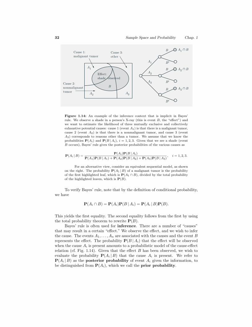
Figure 1.14: An example of the inference context that is implicit in Bayes’rule. We observe a shade in a person’s X-ray (this is event B, the “effect”) andwe want to estimate the likelihood of three mutually exclusive and collectivelyexhaustive potential causes: cause 1 (event A1) is that there is a malignant tumor,cause 2 (event A2) is that there is a nonmalignant tumor, and cause 3 (eventA3) corresponds to reasons other than a tumor. We assume that we know theprobabilities P(Ai) and P(B |Ai), i = 1, 2, 3. Given that we see a shade (eventB occurs), Bayes’ rule gives the posterior probabilities of the various causes as
P(Ai |B) =P(Ai)P(B |Ai)
P(A1)P(B |A1) + P(A2)P(B |A2) + P(A3)P(B |A3), i = 1, 2, 3.
For an alternative view, consider an equivalent sequential model, as shownon the right. The probability P(A1 |B) of a malignant tumor is the probabilityof the first highlighted leaf, which is P(A1 ∩ B), divided by the total probabilityof the highlighted leaves, which is P(B).
To verify Bayes’ rule, note that by the definition of conditional probability,we have
P(Ai ∩ B) = P(Ai)P(B |Ai) = P(Ai |B)P(B).
This yields the first equality. The second equality follows from the first by usingthe total probability theorem to rewrite P(B).
Bayes’ rule is often used for inference. There are a number of “causes”that may result in a certain “effect.” We observe the effect, and we wish to inferthe cause. The events A1, . . . , An are associated with the causes and the event Brepresents the effect. The probability P(B |Ai) that the effect will be observedwhen the cause Ai is present amounts to a probabilistic model of the cause-effectrelation (cf. Fig. 1.14). Given that the effect B has been observed, we wish toevaluate the probability P(Ai |B) that the cause Ai is present. We refer toP(Ai |B) as the posterior probability of event Ai given the information, tobe distinguished from P(Ai), which we call the prior probability.
Sec. 1.4 Total Probability Theorem and Bayes’ Rule 33
Example 1.16. Let us return to the radar detection problem of Example 1.9 andFig. 1.9. Let
A = {an aircraft is present},B = {the radar generates an alarm}.
We are given that
P(A) = 0.05, P(B |A) = 0.99, P(B |Ac) = 0.1.
Applying Bayes’ rule, with A1 = A and A2 = Ac, we obtain
P(aircraft present | alarm) = P(A |B)
=P(A)P(B |A)
P(B)
=P(A)P(B |A)
P(A)P(B |A) + P(Ac)P(B |Ac)
=0.05 · 0.99
0.05 · 0.99 + 0.95 · 0.1
≈ 0.3426.
Example 1.17. Let us return to the chess problem of Example 1.13. Here, Ai isthe event of getting an opponent of type i, and
P(A1) = 0.5, P(A2) = 0.25, P(A3) = 0.25.
Also, B is the event of winning, and
P(B |A1) = 0.3, P(B |A2) = 0.4, P(B |A3) = 0.5.
Suppose that you win. What is the probability P(A1 |B) that you had an opponentof type 1?
Using Bayes’ rule, we have
P(A1 |B) =P(A1)P(B |A1)
P(A1)P(B |A1) + P(A2)P(B |A2) + P(A3)P(B |A3)
=0.5 · 0.3
0.5 · 0.3 + 0.25 · 0.4 + 0.25 · 0.5
= 0.4.
Example 1.18. The False-Positive Puzzle. A test for a certain rare disease isassumed to be correct 95% of the time: if a person has the disease, the test resultsare positive with probability 0.95, and if the person does not have the disease,the test results are negative with probability 0.95. A random person drawn from
34 Sample Space and Probability Chap. 1
a certain population has probability 0.001 of having the disease. Given that theperson just tested positive, what is the probability of having the disease?
If A is the event that the person has the disease, and B is the event that thetest results are positive, the desired probability, P(A |B), is
P(A |B) =P(A)P(B |A)
P(A)P(B |A) + P(Ac)P(B |Ac)
=0.001 · 0.95
0.001 · 0.95 + 0.999 · 0.05
= 0.0187.
Note that even though the test was assumed to be fairly accurate, a person who hastested positive is still very unlikely (less than 2%) to have the disease. Accordingto The Economist (February 20th, 1999), 80% of those questioned at a leadingAmerican hospital substantially missed the correct answer to a question of thistype; most of them thought that the probability that the person has the diseaseis 0.95!
1.5 INDEPENDENCE
We have introduced the conditional probability P(A |B) to capture the partialinformation that event B provides about event A. An interesting and importantspecial case arises when the occurrence of B provides no such information anddoes not alter the probability that A has occurred, i.e.,
P(A |B) = P(A).
When the above equality holds, we say that A is independent of B. Note thatby the definition P(A |B) = P(A ∩ B)/P(B), this is equivalent to
P(A ∩ B) = P(A)P(B).
We adopt this latter relation as the definition of independence because it can beused even when P(B) = 0, in which case P(A |B) is undefined. The symmetryof this relation also implies that independence is a symmetric property; that is,if A is independent of B, then B is independent of A, and we can unambiguouslysay that A and B are independent events.
Independence is often easy to grasp intuitively. For example, if the occur-rence of two events is governed by distinct and noninteracting physical processes,such events will turn out to be independent. On the other hand, independenceis not easily visualized in terms of the sample space. A common first thoughtis that two events are independent if they are disjoint, but in fact the oppo-site is true: two disjoint events A and B with P(A) > 0 and P(B) > 0 arenever independent, since their intersection A∩B is empty and has probability 0.
Sec. 1.5 Independence 35
For example, an event A and its complement Ac are not independent [unlessP(A) = 0 or P(A) = 1], since knowledge that A has occurred provides preciseinformation about whether Ac has occurred.
Example 1.19. Consider an experiment involving two successive rolls of a 4-sideddie in which all 16 possible outcomes are equally likely and have probability 1/16.
(a) Are the events
Ai = {1st roll results in i}, Bj = {2nd roll results in j},
independent? We have
P(Ai ∩ Bj) = P(the outcome of the two rolls is (i, j)
)=
1
16,
P(Ai) =number of elements of Ai
total number of possible outcomes=
4
16,
P(Bj) =number of elements of Bj
total number of possible outcomes=
4
16.
We observe that P(Ai ∩Bj) = P(Ai)P(Bj), and the independence of Ai andBj is verified. Thus, our choice of the discrete uniform probability law impliesthe independence of the two rolls.
(b) Are the events
A = {1st roll is a 1}, B = {sum of the two rolls is a 5},
independent? The answer here is not quite obvious. We have
P(A ∩ B) = P(the result of the two rolls is (1,4)
)=
1
16,
and also
P(A) =number of elements of A
total number of possible outcomes=
4
16.
The event B consists of the outcomes (1,4), (2,3), (3,2), and (4,1), and
P(B) =number of elements of B
total number of possible outcomes=
4
16.
Thus, we see that P(A ∩ B) = P(A)P(B), and the events A and B areindependent.
(c) Are the events
A = {maximum of the two rolls is 2}, B = {minimum of the two rolls is 2},
36 Sample Space and Probability Chap. 1
independent? Intuitively, the answer is “no” because the minimum of thetwo rolls conveys some information about the maximum. For example, if theminimum is 2, the maximum cannot be 1. More precisely, to verify that Aand B are not independent, we calculate
P(A ∩ B) = P(the result of the two rolls is (2,2)
)=
1
16,
and also
P(A) =number of elements of A
total number of possible outcomes=
3
16,
P(B) =number of elements of B
total number of possible outcomes=
5
16.
We have P(A)P(B) = 15/(16)2, so that P(A ∩ B) �= P(A)P(B), and A andB are not independent.
We finally note that, as mentioned earlier, if A and B are independent, theoccurrence of B does not provide any new information on the probability of Aoccurring. It is then intuitive that the non-occurrence of B should also provideno information on the probability of A. Indeed, it can be verified that if A andB are independent, the same holds true for A and Bc (see the end-of-chapterproblems).
Conditional Independence
We noted earlier that the conditional probabilities of events, conditioned ona particular event, form a legitimate probability law. We can thus talk aboutindependence of various events with respect to this conditional law. In particular,given an event C, the events A and B are called conditionally independentif
P(A ∩ B |C) = P(A |C)P(B |C).
To derive an alternative characterization of conditional independence, we use thedefinition of the conditional probability and the multiplication rule, to write
P(A ∩ B |C) =P(A ∩ B ∩ C)
P(C)
=P(C)P(B |C)P(A |B ∩ C)
P(C)
= P(B |C)P(A |B ∩ C).
We now compare the preceding two expressions, and after eliminating the com-mon factor P(B |C), assumed nonzero, we see that conditional independence isthe same as the condition
P(A |B ∩ C) = P(A |C).
Sec. 1.5 Independence 37
In words, this relation states that if C is known to have occurred, the additionalknowledge that B also occurred does not change the probability of A.
Interestingly, independence of two events A and B with respect to theunconditional probability law, does not imply conditional independence, andvice versa, as illustrated by the next two examples.
Example 1.20. Consider two independent fair coin tosses, in which all four possibleoutcomes are equally likely. Let
H1 = {1st toss is a head},H2 = {2nd toss is a head},D = {the two tosses have different results}.
The events H1 and H2 are (unconditionally) independent. But
P(H1 |D) =1
2, P(H2 |D) =
1
2, P(H1 ∩ H2 |D) = 0,
so that P(H1 ∩ H2 |D) �= P(H1 |D)P(H2 |D), and H1, H2 are not conditionallyindependent.
This example can be generalized. For any probabilistic model, let A and B beindependent events, and let C be an event such that P(C) > 0, P(A |C) > 0, andP(B |C) > 0, while A ∩ B ∩ C is empty. Then, A and B cannot be conditionallyindependent (given C) since P(A ∩ B |C) = 0 while P(A |C)P(B |C) > 0.
Example 1.21. There are two coins, a blue and a red one. We choose one ofthe two at random, each being chosen with probability 1/2, and proceed with twoindependent tosses. The coins are biased: with the blue coin, the probability ofheads in any given toss is 0.99, whereas for the red coin it is 0.01.
Let B be the event that the blue coin was selected. Let also Hi be the eventthat the ith toss resulted in heads. Given the choice of a coin, the events H1 andH2 are independent, because of our assumption of independent tosses. Thus,
P(H1 ∩ H2 |B) = P(H1 |B)P(H2 |B) = 0.99 · 0.99.
On the other hand, the events H1 and H2 are not independent. Intuitively, if weare told that the first toss resulted in heads, this leads us to suspect that the bluecoin was selected, in which case, we expect the second toss to also result in heads.Mathematically, we use the total probability theorem to obtain
P(H1) = P(B)P(H1 |B) + P(Bc)P(H1 |Bc) =1
2· 0.99 +
1
2· 0.01 =
1
2,
as should be expected from symmetry considerations. Similarly, we have P(H2) =1/2. Now notice that
P(H1 ∩ H2) = P(B)P(H1 ∩ H2 |B) + P(Bc)P(H1 ∩ H2 |Bc)
=1
2· 0.99 · 0.99 +
1
2· 0.01 · 0.01 ≈ 1
2.
38 Sample Space and Probability Chap. 1
Thus, P(H1 ∩H2) �= P(H1)P(H2), and the events H1 and H2 are dependent, eventhough they are conditionally independent given B.
We now summarize.
Independence
• Two events A and B are said to be independent if
P(A ∩ B) = P(A)P(B).
If in addition, P(B) > 0, independence is equivalent to the condition
P(A |B) = P(A).
• If A and B are independent, so are A and Bc.
• Two events A and B are said to be conditionally independent,given another event C with P(C) > 0, if
P(A ∩ B |C) = P(A |C)P(B |C).
If in addition, P(B ∩ C) > 0, conditional independence is equivalentto the condition
P(A |B ∩ C) = P(A |C).
• Independence does not imply conditional independence, and vice versa.
Independence of a Collection of Events
The definition of independence can be extended to multiple events.
Definition of Independence of Several Events
We say that the events A1, A2, . . . , An are independent if
P
(⋂i∈S
Ai
)=
∏i∈S
P(Ai), for every subset S of {1, 2, . . . , n}.
Sec. 1.5 Independence 39
For the case of three events, A1, A2, and A3, independence amounts tosatisfying the four conditions
P(A1 ∩ A2) = P(A1)P(A2),P(A1 ∩ A3) = P(A1)P(A3),P(A2 ∩ A3) = P(A2)P(A3),
P(A1 ∩ A2 ∩ A3) = P(A1)P(A2)P(A3).
The first three conditions simply assert that any two events are independent,a property known as pairwise independence. But the fourth condition isalso important and does not follow from the first three. Conversely, the fourthcondition does not imply the first three; see the two examples that follow.
Example 1.22. Pairwise Independence does not Imply Independence.Consider two independent fair coin tosses, and the following events:
H1 = {1st toss is a head},H2 = {2nd toss is a head},D = {the two tosses have different results}.
The events H1 and H2 are independent, by definition. To see that H1 and D areindependent, we note that
P(D |H1) =P(H1 ∩ D)
P(H1)=
1/4
1/2=
1
2= P(D).
Similarly, H2 and D are independent. On the other hand, we have
P(H1 ∩ H2 ∩ D) = 0 �= 1
2· 1
2· 1
2= P(H1)P(H2)P(D),
and these three events are not independent.
Example 1.23. The Equality P(A1 ∩ A2 ∩ A3) = P(A1)P(A2)P(A3) is notEnough for Independence. Consider two independent rolls of a fair six-sideddie, and the following events:
A = {1st roll is 1, 2, or 3},B = {1st roll is 3, 4, or 5},C = {the sum of the two rolls is 9}.
We have
P(A ∩ B) =1
6�= 1
2· 1
2= P(A)P(B),
P(A ∩ C) =1
36�= 1
2· 4
36= P(A)P(C),
P(B ∩ C) =1
12�= 1
2· 4
36= P(B)P(C).
40 Sample Space and Probability Chap. 1
Thus the three events A, B, and C are not independent, and indeed no two of theseevents are independent. On the other hand, we have
P(A ∩ B ∩ C) =1
36=
1
2· 1
2· 4
36= P(A)P(B)P(C).
The intuition behind the independence of a collection of events is anal-ogous to the case of two events. Independence means that the occurrence ornon-occurrence of any number of the events from that collection carries noinformation on the remaining events or their complements. For example, if theevents A1, A2, A3, A4 are independent, one obtains relations such as
P(A1 ∪ A2 |A3 ∩ A4) = P(A1 ∪ A2)
orP(A1 ∪ Ac
2 |Ac3 ∩ A4) = P(A1 ∪ Ac
2);
see the end-of-chapter problems.
Reliability
In probabilistic models of complex systems involving several components, it isoften convenient to assume that the behaviors of the components are uncoupled(independent). This typically simplifies the calculations and the analysis, asillustrated in the following example.
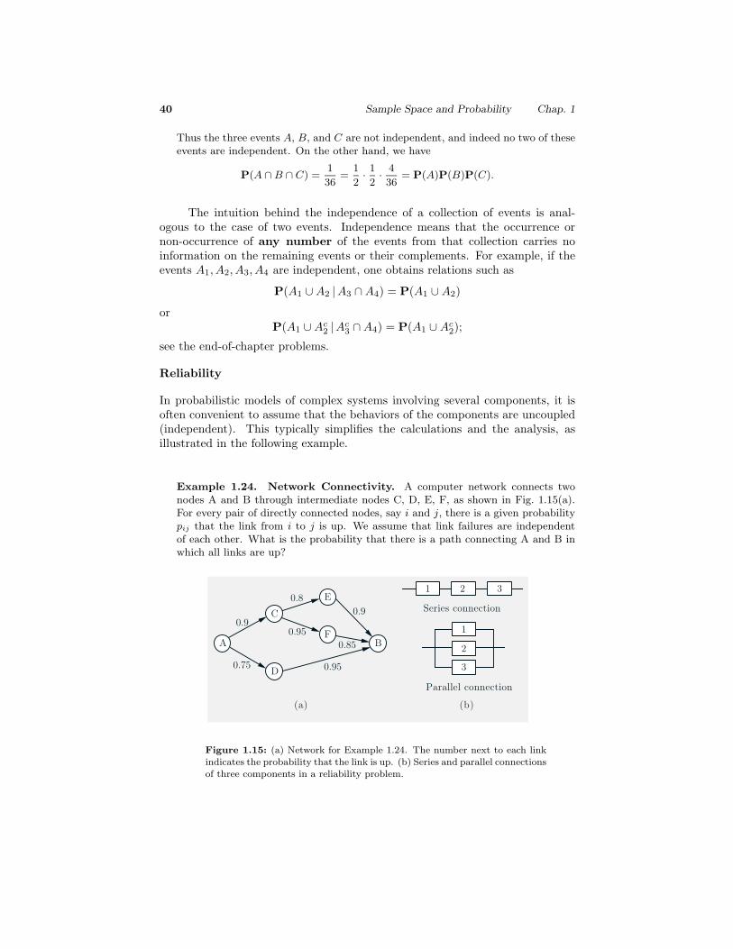
Example 1.24. Network Connectivity. A computer network connects twonodes A and B through intermediate nodes C, D, E, F, as shown in Fig. 1.15(a).For every pair of directly connected nodes, say i and j, there is a given probabilitypij that the link from i to j is up. We assume that link failures are independentof each other. What is the probability that there is a path connecting A and B inwhich all links are up?
F
(b)
Series connection
1 2 3
Parallel connection
1
2
3
(a)
A B
C
E
D
0.9
0.8
0.95
0.9
0.85
0.75
0.95
Figure 1.15: (a) Network for Example 1.24. The number next to each linkindicates the probability that the link is up. (b) Series and parallel connectionsof three components in a reliability problem.
Sec. 1.5 Independence 41
This is a typical problem of assessing the reliability of a system consisting ofcomponents that can fail independently. Such a system can often be divided intosubsystems, where each subsystem consists in turn of several components that areconnected either in series or in parallel; see Fig. 1.15(b).
Let a subsystem consist of components 1, 2, . . . , m, and let pi be the prob-ability that component i is up (“succeeds”). Then, a series subsystem succeedsif all of its components are up, so its probability of success is the product of theprobabilities of success of the corresponding components, i.e.,
P(series subsystem succeeds) = p1p2 · · · pm.
A parallel subsystem succeeds if any one of its components succeeds, so its prob-ability of failure is the product of the probabilities of failure of the correspondingcomponents, i.e.,
P(parallel subsystem succeeds) = 1 − P(parallel subsystem fails)
= 1 − (1 − p1)(1 − p2) · · · (1 − pm).
Returning now to the network of Fig. 1.15(a), we can calculate the probabil-ity of success (a path from A to B is available) sequentially, using the precedingformulas, and starting from the end. Let us use the notation X → Y to denote theevent that there is a (possibly indirect) connection from node X to node Y . Then,
P(C → B) = 1 −(1 − P(C → E and E → B)
)(1 − P(C → F and F → B)
)= 1 − (1 − pCEpEB)(1 − pCF pFB)
= 1 − (1 − 0.8 · 0.9)(1 − 0.95 · 0.85)
= 0.946,
P(A → C and C → B) = P(A → C)P(C → B) = 0.9 · 0.946 = 0.851,
P(A → D and D → B) = P(A → D)P(D → B) = 0.75 · 0.95 = 0.712,
and finally we obtain the desired probability
P(A → B) = 1 −(1 − P(A → C and C → B)
)(1 − P(A → D and D → B)
)= 1 − (1 − 0.851)(1 − 0.712)
= 0.957.
Independent Trials and the Binomial Probabilities
If an experiment involves a sequence of independent but identical stages, we saythat we have a sequence of independent trials. In the special case where thereare only two possible results at each stage, we say that we have a sequence ofindependent Bernoulli trials. The two possible results can be anything, e.g.,“it rains” or “it doesn’t rain,” but we will often think in terms of coin tosses andrefer to the two results as “heads” (H) and “tails” (T ).
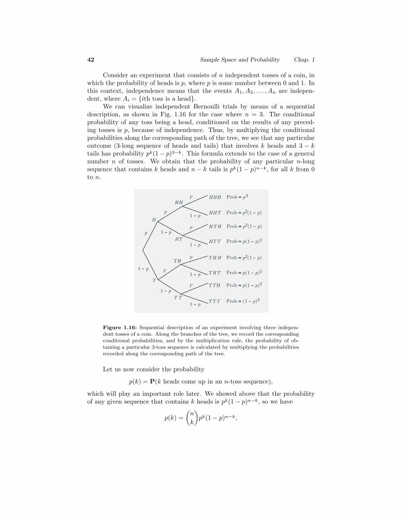
42 Sample Space and Probability Chap. 1
Consider an experiment that consists of n independent tosses of a coin, inwhich the probability of heads is p, where p is some number between 0 and 1. Inthis context, independence means that the events A1, A2, . . . , An are indepen-dent, where Ai = {ith toss is a head}.
We can visualize independent Bernoulli trials by means of a sequentialdescription, as shown in Fig. 1.16 for the case where n = 3. The conditionalprobability of any toss being a head, conditioned on the results of any preced-ing tosses is p, because of independence. Thus, by multiplying the conditionalprobabilities along the corresponding path of the tree, we see that any particularoutcome (3-long sequence of heads and tails) that involves k heads and 3 − ktails has probability pk(1− p)3−k. This formula extends to the case of a generalnumber n of tosses. We obtain that the probability of any particular n-longsequence that contains k heads and n − k tails is pk(1 − p)n−k, for all k from 0to n.
p
p
p
p
p
p
p
HH
HT
TH
T T
H
T
1 − p
1 − p
1 − p
1 − p
1 − p
1 − p
1 − p
HHH
HH T
H T H
HT T
T H H
T H T
T TH
T T T
Prob = p2(1 − p)
Prob = p3
Prob = p(1 − p)2
Prob = p2(1 − p)
Prob = p2(1 − p)
Prob = p(1 − p)2
Prob = p(1 − p)2
Prob = (1 − p)3
Figure 1.16: Sequential description of an experiment involving three indepen-dent tosses of a coin. Along the branches of the tree, we record the correspondingconditional probabilities, and by the multiplication rule, the probability of ob-taining a particular 3-toss sequence is calculated by multiplying the probabilitiesrecorded along the corresponding path of the tree.
Let us now consider the probability
p(k) = P(k heads come up in an n-toss sequence),
which will play an important role later. We showed above that the probabilityof any given sequence that contains k heads is pk(1 − p)n−k, so we have
p(k) =(
n
k
)pk(1 − p)n−k,
Sec. 1.5 Independence 43
where we use the notation(n
k
)= number of distinct n-toss sequences that contain k heads.
The numbers(nk
)(read as “n choose k”) are known as the binomial coeffi-
cients, while the probabilities p(k) are known as the binomial probabilities.Using a counting argument, to be given in Section 1.6, we can show that(
n
k
)=
n!k! (n − k)!
, k = 0, 1, . . . , n,
where for any positive integer i we have
i! = 1 · 2 · · · (i − 1) · i,
and, by convention, 0! = 1. An alternative verification is sketched in the end-of-chapter problems. Note that the binomial probabilities p(k) must add to 1, thusshowing the binomial formula
n∑k=0
(n
k
)pk(1 − p)n−k = 1.
Example 1.25. Grade of Service. An internet service provider has installed cmodems to serve the needs of a population of n dialup customers. It is estimatedthat at a given time, each customer will need a connection with probability p,independent of the others. What is the probability that there are more customersneeding a connection than there are modems?
Here we are interested in the probability that more than c customers simul-taneously need a connection. It is equal to
n∑k=c+1
p(k),
where
p(k) =
(n
k
)pk(1 − p)n−k
are the binomial probabilities. For instance, if n = 100, p = 0.1, and c = 15, theprobability of interest turns out to be 0.0399.
This example is typical of problems of sizing a facility to serve the needsof a homogeneous population, consisting of independently acting customers. Theproblem is to select the facility size to guarantee a certain probability (sometimescalled grade of service) that no user is left unserved.
44 Sample Space and Probability Chap. 1
1.6 COUNTING
The calculation of probabilities often involves counting the number of outcomesin various events. We have already seen two contexts where such counting arises.
(a) When the sample space Ω has a finite number of equally likely outcomes,so that the discrete uniform probability law applies. Then, the probabilityof any event A is given by
P(A) =number of elements of A
number of elements of Ω,
and involves counting the elements of A and of Ω.
(b) When we want to calculate the probability of an event A with a finitenumber of equally likely outcomes, each of which has an already knownprobability p. Then the probability of A is given by
P(A) = p · (number of elements of A),
and involves counting the number of elements of A. An example of this typeis the calculation of the probability of k heads in n coin tosses (the binomialprobabilities). We saw in the preceding section that the probability of eachdistinct sequence involving k heads is easily obtained, but the calculationof the number of all such sequences, to be presented shortly, requires somethought.
While counting is in principle straightforward, it is frequently challenging;the art of counting constitutes a large portion of the field of combinatorics. Inthis section, we present the basic principle of counting and apply it to a numberof situations that are often encountered in probabilistic models.
The Counting Principle
The counting principle is based on a divide-and-conquer approach, whereby thecounting is broken down into stages through the use of a tree. For example,consider an experiment that consists of two consecutive stages. The possibleresults of the first stage are a1, a2, . . . , am; the possible results of the secondstage are b1, b2, . . . , bn. Then, the possible results of the two-stage experimentare all possible ordered pairs (ai, bj), i = 1, . . . , m, j = 1, . . . , n. Note that thenumber of such ordered pairs is equal to mn. This observation can be generalizedas follows (see also Fig. 1.17).
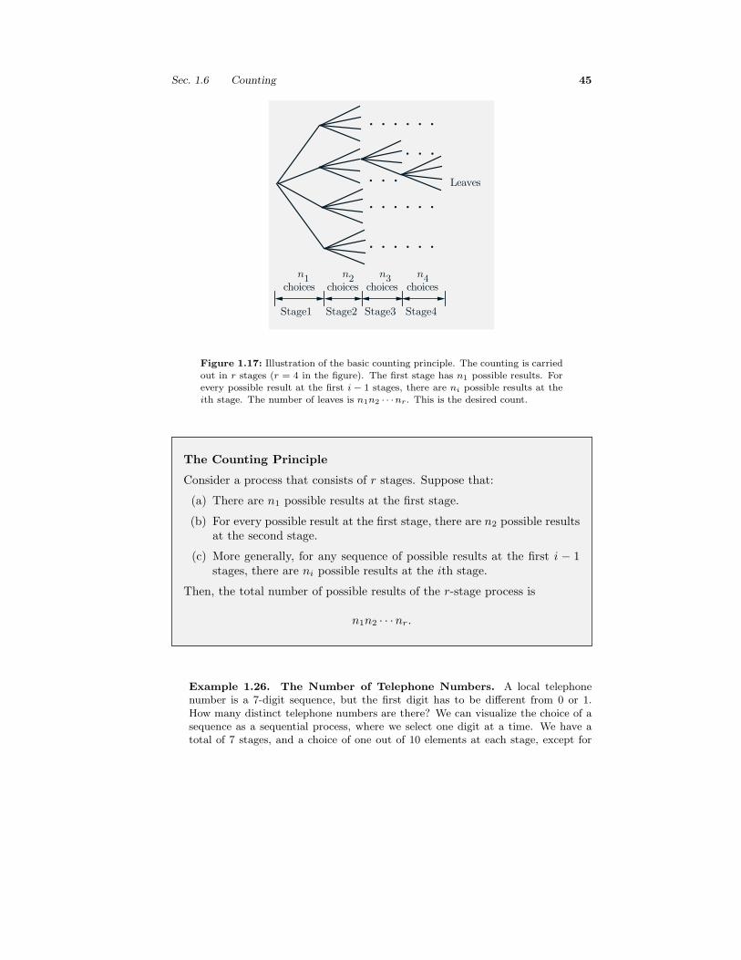
Sec. 1.6 Counting 45
Leaves
. . . . . .
. . . . . .
. . . . . .
. . .
Stage1 Stage2 Stage3 Stage4
choices choices choices choicesn1 n2 n3 n4
. . .
Figure 1.17: Illustration of the basic counting principle. The counting is carriedout in r stages (r = 4 in the figure). The first stage has n1 possible results. Forevery possible result at the first i − 1 stages, there are ni possible results at theith stage. The number of leaves is n1n2 · · ·nr. This is the desired count.
The Counting Principle
Consider a process that consists of r stages. Suppose that:
(a) There are n1 possible results at the first stage.
(b) For every possible result at the first stage, there are n2 possible resultsat the second stage.
(c) More generally, for any sequence of possible results at the first i − 1stages, there are ni possible results at the ith stage.
Then, the total number of possible results of the r-stage process is
n1n2 · · ·nr.
Example 1.26. The Number of Telephone Numbers. A local telephonenumber is a 7-digit sequence, but the first digit has to be different from 0 or 1.How many distinct telephone numbers are there? We can visualize the choice of asequence as a sequential process, where we select one digit at a time. We have atotal of 7 stages, and a choice of one out of 10 elements at each stage, except for
46 Sample Space and Probability Chap. 1
the first stage where we only have 8 choices. Therefore, the answer is
8 · 10 · 10 · · · 10︸ ︷︷ ︸6 times
= 8 · 106.
Example 1.27. The Number of Subsets of an n-Element Set. Consideran n-element set {s1, s2, . . . , sn}. How many subsets does it have (including itselfand the empty set)? We can visualize the choice of a subset as a sequential processwhere we examine one element at a time and decide whether to include it in the setor not. We have a total of n stages, and a binary choice at each stage. Thereforethe number of subsets is
2 · 2 · · · 2︸ ︷︷ ︸n times
= 2n.
It should be noted that the Counting Principle remains valid even if eachfirst-stage result leads to a different set of potential second-stage results, etc. Theonly requirement is that the number of possible second-stage results is constant,regardless of the first-stage result.
In what follows, we will focus primarily on two types of counting argumentsthat involve the selection of k objects out of a collection of n objects. If the orderof selection matters, the selection is called a permutation, and otherwise, it iscalled a combination. We will then discuss a more general type of counting,involving a partition of a collection of n objects into multiple subsets.
k-permutations
We start with n distinct objects, and let k be some positive integer, with k ≤ n.We wish to count the number of different ways that we can pick k out of thesen objects and arrange them in a sequence, i.e., the number of distinct k-objectsequences. We can choose any of the n objects to be the first one. Having chosenthe first, there are only n− 1 possible choices for the second; given the choice ofthe first two, there only remain n − 2 available objects for the third stage, etc.When we are ready to select the last (the kth) object, we have already chosenk − 1 objects, which leaves us with n − (k − 1) choices for the last one. By theCounting Principle, the number of possible sequences, called k-permutations,is
n(n − 1) · · · (n − k + 1) =n(n − 1) · · · (n − k + 1)(n − k) · · · 2 · 1
(n − k) · · · 2 · 1
=n!
(n − k)!.
In the special case where k = n, the number of possible sequences, simply calledpermutations, is
n(n − 1)(n − 2) · · · 2 · 1 = n!.
(Let k = n in the formula for the number of k-permutations, and recall theconvention 0! = 1.)
Sec. 1.6 Counting 47
Example 1.28. Let us count the number of words that consist of four distinctletters. This is the problem of counting the number of 4-permutations of the 26letters in the alphabet. The desired number is
n!
(n − k)!=
26!
22!= 26 · 25 · 24 · 23 = 358, 800.
The count for permutations can be combined with the Counting Principleto solve more complicated counting problems.
Example 1.29. You have n1 classical music CDs, n2 rock music CDs, and n3
country music CDs. In how many different ways can you arrange them so that theCDs of the same type are contiguous?
We break down the problem in two stages, where we first select the order ofthe CD types, and then the order of the CDs of each type. There are 3! ordered se-quences of the types of CDs (such as classical/rock/country, rock/country/classical,etc.), and there are n1! (or n2!, or n3!) permutations of the classical (or rock, orcountry, respectively) CDs. Thus for each of the 3! CD type sequences, there aren1! n2! n3! arrangements of CDs, and the desired total number is 3! n1! n2! n3!.
Suppose now that you offer to give ki out of the ni CDs of each type i to afriend, where ki < ni, i = 1, 2, 3. What is the number of all possible arrangementsof the CDs that you are left with? The solution is similar, except that the number of(ni − ki)-permutations of CDs of type i replaces ni! in the estimate, so the numberof possible arrangements is
3! · n1!
k1!· n2!
k2!· n3!
k3!.
Combinations
There are n people and we are interested in forming a committee of k. Howmany different committees are possible? More abstractly, this is the same as theproblem of counting the number of k-element subsets of a given n-element set.Notice that forming a combination is different than forming a k-permutation,because in a combination there is no ordering of the selected elements.For example, whereas the 2-permutations of the letters A, B, C, and D are
AB, BA, AC, CA, AD, DA, BC, CB, BD, DB, CD, DC,
the combinations of two out of these four letters are
AB, AC, AD, BC, BD, CD.
In the preceding example, the combinations are obtained from the per-mutations by grouping together “duplicates”; for example, AB and BA are not
48 Sample Space and Probability Chap. 1
viewed as distinct, and are both associated with the combination AB. This rea-soning can be generalized: each combination is associated with k! “duplicate”k-permutations, so the number n!/(n − k)! of k-permutations is equal to thenumber of combinations times k!. Hence, the number of possible combinations,is equal to
n!k! (n − k)!
.
Let us now relate the above expression to the binomial coefficient, whichwas denoted by
(nk
)and was defined in the preceding section as the number of
n-toss sequences with k heads. We note that specifying an n-toss sequence withk heads is the same as selecting k elements (those that correspond to heads) outof the n-element set of tosses, i.e., a combination of k out of n objects. Hence,the binomial coefficient is also given by the same formula and we have(
n
k
)=
n!k! (n − k)!
.
Example 1.30. The number of combinations of two out of the four letters A, B,C, and D is found by letting n = 4 and k = 2. It is(
4
2
)=
4!
2! 2!= 6,
consistent with the listing given earlier.
It is worth observing that counting arguments sometimes lead to formulasthat are rather difficult to derive algebraically. One example is the binomialformula
n∑k=0
(n
k
)pk(1 − p)n−k = 1,
discussed in Section 1.5. In the special case where p = 1/2, this formula becomes
n∑k=0
(n
k
)= 2n,
and admits the following simple interpretation. Since(nk
)is the number of k-
element subsets of a given n-element subset, the sum over k of(nk
)counts the
number of subsets of all possible cardinalities. It is therefore equal to the numberof all subsets of an n-element set, which is 2n.
Example 1.31. Consider a group of n persons, and clubs that consist of a specialperson from the group (the club leader) and a number (possibly zero) of additional
Sec. 1.6 Counting 49
club members. Let us count the number of possible clubs of this type in two differentways, thereby obtaining an algebraic identity.
There are n choices for club leader. Once the leader is chosen, we are leftwith a set of n − 1 available persons, and we are free to choose any of the 2n−1
subsets. Thus the number of possible clubs is n2n−1.Alternatively, for fixed k, we can form a k-person club by first selecting k out
of the n available persons [there are(
nk
)choices]. We can then select one of the
members to be the leader (there are k choices). By adding over all possible clubsizes k, we obtain the number of possible clubs as
∑n
k=1k(
nk
), thereby showing the
identityn∑
k=1
k
(n
k
)= n2n−1.
Partitions
Recall that a combination is a choice of k elements out of an n-element setwithout regard to order. Thus, a combination can be viewed as a partition ofthe set in two: one part contains k elements and the other contains the remainingn − k. We now generalize by considering partitions into more than two subsets.
We are given an n-element set and nonnegative integers n1, n2, . . . , nr,whose sum is equal to n. We consider partitions of the set into r disjoint subsets,with the ith subset containing exactly ni elements. Let us count in how manyways this can be done.
We form the subsets one at a time. We have(
nn1
)ways of forming the
first subset. Having formed the first subset, we are left with n − n1 elements.We need to choose n2 of them in order to form the second subset, and we have(n−n1
n2
)choices, etc. Using the Counting Principle for this r-stage process, the
total number of choices is(n
n1
)(n − n1
n2
)(n − n1 − n2
n3
)· · ·
(n − n1 − · · · − nr−1
nr
),
which is equal to
n!n1! (n − n1)!
· (n − n1)!n2! (n − n1 − n2)!
· · · (n − n1 − · · · − nr−1)!(n − n1 − · · · − nr−1 − nr)!nr!
.
We note that several terms cancel and we are left with
n!n1!n2! · · ·nr!
.
This is called the multinomial coefficient and is usually denoted by(n
n1, n2, . . . , nr
).
50 Sample Space and Probability Chap. 1
Example 1.32. Anagrams. How many different words (letter sequences) can beobtained by rearranging the letters in the word TATTOO? There are six positionsto be filled by the available letters. Each rearrangement corresponds to a partitionof the set of the six positions into a group of size 3 (the positions that get the letterT), a group of size 1 (the position that gets the letter A), and a group of size 2 (thepositions that get the letter O). Thus, the desired number is
6!
1! 2! 3!=
1 · 2 · 3 · 4 · 5 · 61 · 1 · 2 · 1 · 2 · 3 = 60.
It is instructive to derive this answer using an alternative argument. (Thisargument can also be used to rederive the multinomial coefficient formula; seethe end-of-chapter problems.) Let us write TATTOO in the form T1AT2T3O1O2
pretending for a moment that we are dealing with 6 distinguishable objects. These6 objects can be rearranged in 6! different ways. However, any of the 3! possiblepermutations of T1, T2, and T3, as well as any of the 2! possible permutations ofO1 and O2, lead to the same word. Thus, when the subscripts are removed, thereare only 6!/(3! 2!) different words.
Example 1.33. A class consisting of 4 graduate and 12 undergraduate studentsis randomly divided into four groups of 4. What is the probability that each groupincludes a graduate student? This is the same as Example 1.11 in Section 1.3, butwe will now obtain the answer using a counting argument.
We first determine the nature of the sample space. A typical outcome is aparticular way of partitioning the 16 students into four groups of 4. We take theterm “randomly” to mean that every possible partition is equally likely, so that theprobability question can be reduced to one of counting.
According to our earlier discussion, there are(16
4, 4, 4, 4
)=
16!
4! 4! 4! 4!
different partitions, and this is the size of the sample space.Let us now focus on the event that each group contains a graduate student.
Generating an outcome with this property can be accomplished in two stages:
(a) Take the four graduate students and distribute them to the four groups; thereare four choices for the group of the first graduate student, three choices forthe second, two for the third. Thus, there is a total of 4! choices for this stage.
(b) Take the remaining 12 undergraduate students and distribute them to thefour groups (3 students in each). This can be done in(
12
3, 3, 3, 3
)=
12!
3! 3! 3! 3!
different ways.
By the Counting Principle, the event of interest can occur in
4! 12!
3! 3! 3! 3!
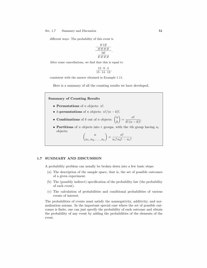
Sec. 1.7 Summary and Discussion 51
different ways. The probability of this event is
4! 12!
3! 3! 3! 3!
16!
4! 4! 4! 4!
.
After some cancellations, we find that this is equal to
12 · 8 · 415 · 14 · 13 ,
consistent with the answer obtained in Example 1.11.
Here is a summary of all the counting results we have developed.
Summary of Counting Results
• Permutations of n objects: n!.
• k-permutations of n objects: n!/(n − k)!.
• Combinations of k out of n objects:(
n
k
)=
n!k! (n − k)!
.
• Partitions of n objects into r groups, with the ith group having ni
objects: (n
n1, n2, . . . , nr
)=
n!n1!n2! · · ·nr!
.
1.7 SUMMARY AND DISCUSSION
A probability problem can usually be broken down into a few basic steps:
(a) The description of the sample space, that is, the set of possible outcomesof a given experiment.
(b) The (possibly indirect) specification of the probability law (the probabilityof each event).
(c) The calculation of probabilities and conditional probabilities of variousevents of interest.
The probabilities of events must satisfy the nonnegativity, additivity, and nor-malization axioms. In the important special case where the set of possible out-comes is finite, one can just specify the probability of each outcome and obtainthe probability of any event by adding the probabilities of the elements of theevent.
52 Sample Space and Probability Chap. 1
Given a probability law, we are often interested in conditional probabilities,which allow us to reason based on partial information about the outcome ofthe experiment. We can view conditional probabilities as probability laws of aspecial type, under which only outcomes contained in the conditioning event canhave positive conditional probability. Conditional probabilities can be derivedfrom the (unconditional) probability law using the definition P(A |B) = P(A ∩B)/P(B). However, the reverse process is often convenient, that is, first specifysome conditional probabilities that are natural for the real situation that we wishto model, and then use them to derive the (unconditional) probability law.
We have illustrated through examples three methods for calculating prob-abilities:
(a) The counting method. This method applies to the case where the num-ber of possible outcomes is finite, and all outcomes are equally likely. Tocalculate the probability of an event, we count the number of elements ofthe event and divide by the number of elements of the sample space.
(b) The sequential method. This method applies when the experiment has asequential character, and suitable conditional probabilities are specified orcalculated along the branches of the corresponding tree (perhaps using thecounting method). The probabilities of various events are then obtainedby multiplying conditional probabilities along the corresponding paths ofthe tree, using the multiplication rule.
(c) The divide-and-conquer method. Here, the probabilities P(B) of vari-ous events B are obtained from conditional probabilities P(B |Ai), wherethe Ai are suitable events that form a partition of the sample space andhave known probabilities P(Ai). The probabilities P(B) are then obtainedby using the total probability theorem.
Finally, we have focused on a few side topics that reinforce our main themes.We have discussed the use of Bayes’ rule in inference, which is an importantapplication context. We have also discussed some basic principles of countingand combinatorics, which are helpful in applying the counting method.
Problems 53
P R O B L E M S
SECTION 1.1. Sets
Problem 1. Consider rolling a six-sided die. Let A be the set of outcomes where theroll is an even number. Let B be the set of outcomes where the roll is greater than 3.Calculate and compare the sets on both sides of De Morgan’s laws
(A ∪ B)c = Ac ∩ Bc,(A ∩ B
)c= Ac ∪ Bc.
Problem 2. Let A and B be two sets.
(a) Show that
Ac = (Ac ∩ B) ∪ (Ac ∩ Bc), Bc = (A ∩ Bc) ∪ (Ac ∩ Bc).
(b) Show that(A ∩ B)c = (Ac ∩ B) ∪ (Ac ∩ Bc) ∪ (A ∩ Bc).
(c) Consider rolling a fair six-sided die. Let A be the set of outcomes where the rollis an odd number. Let B be the set of outcomes where the roll is less than 4.Calculate the sets on both sides of the equality in part (b), and verify that theequality holds.
Problem 3.* Prove the identity
A ∪(∩∞
n=1 Bn
)= ∩∞
n=1(A ∪ Bn).
Solution. If x belongs to the set on the left, there are two possibilities. Either x ∈ A,in which case x belongs to all of the sets A ∪ Bn, and therefore belongs to the set onthe right. Alternatively, x belongs to all of the sets Bn in which case, it belongs to allof the sets A ∪ Bn, and therefore again belongs to the set on the right.
Conversely, if x belongs to the set on the right, then it belongs to A ∪ Bn for alln. If x belongs to A, then it belongs to the set on the left. Otherwise, x must belongto every set Bn and again belongs to the set on the left.
Problem 4.* Cantor’s diagonalization argument. Show that the unit interval[0, 1] is uncountable, i.e., its elements cannot be arranged in a sequence.
Solution. Any number x in [0, 1] can be represented in terms of its decimal expansion,e.g., 1/3 = 0.3333 · · ·. Note that most numbers have a unique decimal expansion,but there are a few exceptions. For example, 1/2 can be represented as 0.5000 · · · oras 0.49999 · · ·. It can be shown that this is the only kind of exception, i.e., decimalexpansions that end with an infinite string of zeroes or an infinite string of nines.
54 Sample Space and Probability Chap. 1
Suppose, to obtain a contradiction, that the elements of [0, 1] can be arrangedin a sequence x1, x2, x3, . . ., so that every element of [0, 1] appears in the sequence.Consider the decimal expansion of xn:
xn = 0.a1na2
na3n · · · ,
where each digit ain belongs to {0, 1, . . . , 9}. Consider now a number y constructed as
follows. The nth digit of y can be 1 or 2, and is chosen so that it is different from thenth digit of xn. Note that y has a unique decimal expansion since it does not end withan infinite sequence of zeroes or nines. The number y differs from each xn, since it hasa different nth digit. Therefore, the sequence x1, x2, . . . does not exhaust the elementsof [0, 1], contrary to what was assumed. The contradiction establishes that the set [0, 1]is uncountable.
SECTION 1.2. Probabilistic Models
Problem 5. Out of the students in a class, 60% are geniuses, 70% love chocolate,and 40% fall into both categories. Determine the probability that a randomly selectedstudent is neither a genius nor a chocolate lover.
Problem 6. A six-sided die is loaded in a way that each even face is twice as likelyas each odd face. All even faces are equally likely, as are all odd faces. Construct aprobabilistic model for a single roll of this die and find the probability that the outcomeis less than 4.
Problem 7. A four-sided die is rolled repeatedly, until the first time (if ever) that aneven number is obtained. What is the sample space for this experiment?
Problem 8. You enter a special kind of chess tournament, in which you play one gamewith each of three opponents, but you get to choose the order in which you play youropponents, knowing the probability of a win against each. You win the tournament ifyou win two games in a row, and you want to maximize the probability of winning.Show that it is optimal to play the weakest opponent second, and that the order ofplaying the other two opponents does not matter.
Problem 9. A partition of the sample space Ω is a collection of disjoint eventsS1, . . . , Sn such that Ω = ∪n
i=1Si.
(a) Show that for any event A, we have
P(A) =
n∑i=1
P(A ∩ Si).
(b) Use part (a) to show that for any events A, B, and C, we have
P(A) = P(A ∩ B) + P(A ∩ C) + P(A ∩ Bc ∩ Cc) − P(A ∩ B ∩ C).
Problem 10. Show the formula
P((A ∩ Bc) ∪ (Ac ∩ B)
)= P(A) + P(B) − 2P(A ∩ B),
Problems 55
which gives the probability that exactly one of the events A and B will occur. [Comparewith the formula P(A ∪ B) = P(A) + P(B) − P(A ∩ B), which gives the probabilitythat at least one of the events A and B will occur.]
Problem 11.* Bonferroni’s inequality.
(a) Prove that for any two events A and B, we have
P(A ∩ B) ≥ P(A) + P(B) − 1.
(b) Generalize to the case of n events A1, A2, . . . , An, by showing that
P(A1 ∩ A2 ∩ · · · ∩ An) ≥ P(A1) + P(A2) + · · · + P(An) − (n − 1).
Solution. We have P(A ∪ B) = P(A) + P(B) − P(A ∩ B) and P(A ∪ B) ≤ 1, whichimplies part (a). For part (b), we use De Morgan’s law to obtain
1 − P(A1 ∩ · · · ∩ An) = P((A1 ∩ · · · ∩ An)c
)= P(Ac
1 ∪ · · · ∪ Acn)
≤ P(Ac1) + · · · + P(Ac
n)
=(1 − P(A1)
)+ · · · +
(1 − P(An)
)= n − P(A1) − · · · − P(An).
Problem 12.* The inclusion-exclusion formula. Show the following generaliza-tions of the formula
P(A ∪ B) = P(A) + P(B) − P(A ∩ B).
(a) Let A, B, and C be events. Then,
P(A∪B∪C) = P(A)+P(B)+P(C)−P(A∩B)−P(B∩C)−P(A∩C)+P(A∩B∩C).
(b) Let A1, A2, . . . , An be events. Let S1 = {i | 1 ≤ i ≤ n}, S2 = {(i1, i2) | 1 ≤ i1 <i2 ≤ n}, and more generally, let Sm be the set of all m-tuples (i1, . . . , im) ofindices that satisfy 1 ≤ i1 < i2 < · · · < im ≤ n. Then,
P (∪nk=1Ak) =
∑i∈S1
P(Ai) −∑
(i1,i2)∈S2
P(Ai1 ∩ Ai2)
+∑
(i1,i2,i3)∈S3
P(Ai1 ∩ Ai2 ∩ Ai3) − · · · + (−1)n−1P (∩nk=1Ak) .
Solution. (a) We use the formulas P(X ∪ Y ) = P(X) + P(Y ) − P(X ∩ Y ) and(A ∪ B) ∩ C = (A ∩ C) ∪ (B ∩ C). We have
P(A ∪ B ∪ C) = P(A ∪ B) + P(C) − P((A ∪ B) ∩ C
)= P(A ∪ B) + P(C) − P
((A ∩ C) ∪ (B ∩ C)
)= P(A ∪ B) + P(C) − P(A ∩ C) − P(B ∩ C) + P(A ∩ B ∩ C)
= P(A) + P(B) − P(A ∩ B) + P(C) − P(A ∩ C) − P(B ∩ C)
+ P(A ∩ B ∩ C)
= P(A) + P(B) + P(C) − P(A ∩ B) − P(B ∩ C) − P(A ∩ C)
+ P(A ∩ B ∩ C).
56 Sample Space and Probability Chap. 1
(b) Use induction and verify the main induction step by emulating the derivation ofpart (a). For a different approach, see the problems at the end of Chapter 2.
Problem 13.* Continuity property of probabilities.
(a) Let A1, A2, . . . be an infinite sequence of events, which is “monotonically increas-ing,” meaning that An ⊂ An+1 for every n. Let A = ∪∞
n=1An. Show thatP(A) = limn→∞ P(An). Hint: Express the event A as a union of countablymany disjoint sets.
(b) Suppose now that the events are “monotonically decreasing,” i.e., An+1 ⊂ An
for every n. Let A = ∩∞n=1An. Show that P(A) = limn→∞ P(An). Hint: Apply
the result of part (a) to the complements of the events.
(c) Consider a probabilistic model whose sample space is the real line. Show that
P([0,∞)
)= lim
n→∞P
([0, n]
), and lim
n→∞P
([n,∞)
)= 0.
Solution. (a) Let B1 = A1 and, for n ≥ 2, Bn = An ∩ Acn−1. The events Bn are
disjoint, and we have ∪nk=1Bk = An, and ∪∞
k=1Bk = A. We apply the additivity axiomto obtain
P(A) =
∞∑k=1
P(Bk) = limn→∞
n∑k=1
P(Bk) = limn→∞
P(∪nk=1Bk) = lim
n→∞P(An).
(b) Let Cn = Acn and C = Ac. Since An+1 ⊂ An, we obtain Cn ⊂ Cn+1, and the events
Cn are increasing. Furthermore, C = Ac = (∩∞n=1An)c = ∪∞
n=1Acn = ∪∞
n=1Cn. Usingthe result from part (a) for the sequence Cn, we obtain
1 − P(A) = P(Ac) = P(C) = limn→∞
P(Cn) = limn→∞
(1 − P(An)
),
from which we conclude that P(A) = limn→∞ P(An).
(c) For the first equality, use the result from part (a) with An = [0, n] and A = [0,∞).For the second, use the result from part (b) with An = [n,∞) and A = ∩∞
n=1An = Ø.
SECTION 1.3. Conditional Probability
Problem 14. We roll two fair 6-sided dice. Each one of the 36 possible outcomes isassumed to be equally likely.
(a) Find the probability that doubles are rolled.
(b) Given that the roll results in a sum of 4 or less, find the conditional probabilitythat doubles are rolled.
(c) Find the probability that at least one die roll is a 6.
(d) Given that the two dice land on different numbers, find the conditional probabilitythat at least one die roll is a 6.
Problem 15. A coin is tossed twice. Alice claims that the event of two heads is atleast as likely if we know that the first toss is a head than if we know that at least one
Problems 57
of the tosses is a head. Is she right? Does it make a difference if the coin is fair orunfair? How can we generalize Alice’s reasoning?
Problem 16. We are given three coins: one has heads in both faces, the second hastails in both faces, and the third has a head in one face and a tail in the other. Wechoose a coin at random, toss it, and the result is heads. What is the probability thatthe opposite face is tails?
Problem 17. A batch of one hundred items is inspected by testing four randomlyselected items. If one of the four is defective, the batch is rejected. What is theprobability that the batch is accepted if it contains five defectives?
Problem 18. Let A and B be events. Show that P(A∩B |B) = P(A |B), assumingthat P(B) > 0.
SECTION 1.4. Total Probability Theorem and Bayes’ Rule
Problem 19. Alice searches for her term paper in her filing cabinet, which has severaldrawers. She knows that she left her term paper in drawer j with probability pj > 0.The drawers are so messy that even if she correctly guesses that the term paper is indrawer i, the probability that she finds it is only di. Alice searches in a particulardrawer, say drawer i, but the search is unsuccessful. Conditioned on this event, showthat the probability that her paper is in drawer j, is given by
pj
1 − pidi, if j �= i,
pi(1 − di)
1 − pidi, if j = i.
Problem 20. How an inferior player with a superior strategy can gain anadvantage. Boris is about to play a two-game chess match with an opponent, andwants to find the strategy that maximizes his winning chances. Each game ends witheither a win by one of the players, or a draw. If the score is tied at the end of the twogames, the match goes into sudden-death mode, and the players continue to play untilthe first time one of them wins a game (and the match). Boris has two playing styles,timid and bold, and he can choose one of the two at will in each game, no matter whatstyle he chose in previous games. With timid play, he draws with probability pd > 0,and he loses with probability 1− pd. With bold play, he wins with probability pw, andhe loses with probability 1− pw. Boris will always play bold during sudden death, butmay switch style between games 1 and 2.
(a) Find the probability that Boris wins the match for each of the following strategies:(i) Play bold in both games 1 and 2.(ii) Play timid in both games 1 and 2.(iii) Play timid whenever he is ahead in the score, and play bold otherwise.
(b) Assume that pw < 1/2, so Boris is the worse player, regardless of the playingstyle he adopts. Show that with the strategy in (iii) above, and depending onthe values of pw and pd, Boris may have a better than a 50-50 chance to win thematch. How do you explain this advantage?
Problem 21. Two players take turns removing a ball from a jar that initially containsm white and n black balls. The first player to remove a white ball wins. Develop a
58 Sample Space and Probability Chap. 1
recursive formula that allows the convenient computation of the probability that thestarting player wins.
Problem 22. Each of k jars contains m white and n black balls. A ball is randomlychosen from jar 1 and transferred to jar 2, then a ball is randomly chosen from jar 2and transferred to jar 3, etc. Finally, a ball is randomly chosen from jar k. Show thatthe probability that the last ball is white is the same as the probability that the firstball is white, i.e., it is m/(m + n).
Problem 23. We have two jars, each initially containing an equal number of balls.We perform four successive ball exchanges. In each exchange, we pick simultaneouslyand at random a ball from each jar and move it to the other jar. What is the probabilitythat at the end of the four exchanges all the balls will be in the jar where they started?
Problem 24. The prisoner’s dilemma. The release of two out of three prisonershas been announced, but their identity is kept secret. One of the prisoners considersasking a friendly guard to tell him who is the prisoner other than himself that will bereleased, but hesitates based on the following rationale: at the prisoner’s present stateof knowledge, the probability of being released is 2/3, but after he knows the answer,the probability of being released will become 1/2, since there will be two prisoners(including himself) whose fate is unknown and exactly one of the two will be released.What is wrong with this line of reasoning?
Problem 25. A two-envelopes puzzle. You are handed two envelopes, and youknow that each contains a positive integer dollar amount and that the two amounts aredifferent. The values of these two amounts are modeled as constants that are unknown.Without knowing what the amounts are, you select at random one of the two envelopes,and after looking at the amount inside, you may switch envelopes if you wish. A friendclaims that the following strategy will increase above 1/2 your probability of endingup with the envelope with the larger amount: toss a coin repeatedly, let X be equal to1/2 plus the number of tosses required to obtain heads for the first time, and switchif the amount in the envelope you selected is less than the value of X. Is your friendcorrect?
Problem 26. The paradox of induction. Consider a statement whose truth isunknown. If we see many examples that are compatible with it, we are tempted toview the statement as more probable. Such reasoning is often referred to as induc-tive inference (in a philosophical, rather than mathematical sense). Consider now thestatement that “all cows are white.” An equivalent statement is that “everything thatis not white is not a cow.” We then observe several black crows. Our observations areclearly compatible with the statement, but do they make the hypothesis “all cows arewhite” more likely?
To analyze such a situation, we consider a probabilistic model. Let us assumethat there are two possible states of the world, which we model as complementaryevents:
A : all cows are white,
Ac : 50% of all cows are white.
Let p be the prior probability P(A) that all cows are white. We make an observationof a cow or a crow, with probability q and 1 − q, respectively, independent of whether

Problems 59
event A occurs or not. Assume that 0 < p < 1, 0 < q < 1, and that all crows are black.
(a) Given the event B = {a black crow was observed}, what is P(A |B)?
(b) Given the event C = {a white cow was observed}, what is P(A |C)?
Problem 27. Alice and Bob have 2n + 1 coins, each coin with probability of headsequal to 1/2. Bob tosses n+1 coins, while Alice tosses the remaining n coins. Assumingindependent coin tosses, show that the probability that after all coins have been tossed,Bob will have gotten more heads than Alice is 1/2.
Problem 28.* Conditional version of the total probability theorem. LetC1, . . . , Cn be disjoint events that form a partition of the state space. Let also A andB be events such that P(B ∩ Ci) > 0 for all i. Show that
P(A |B) =
n∑i=1
P(Ci |B)P(A |B ∩ Ci).
Solution. We have
P(A ∩ B) =
n∑i=1
P((A ∩ B) ∩ Ci
),
and by using the multiplication rule,
P(((A ∩ B) ∩ Ci
)= P(B)P(Ci |B)P(A |B ∩ Ci).
Combining these two equations, dividing by P(B), and using the formula P(A |B) =P(A ∩ B)/P(B), we obtain the desired result.
Problem 29.* Let A and B be events with P(A) > 0 and P(B) > 0. We say thatan event B suggests an event A if P(A |B) > P(A), and does not suggest event A ifP(A |B) < P(A).
(a) Show that B suggests A if and only if A suggests B.
(b) Assume that P(Bc) > 0. Show that B suggests A if and only if Bc does notsuggest A.
(c) We know that a treasure is located in one of two places, with probabilities β and1−β, respectively, where 0 < β < 1. We search the first place and if the treasureis there, we find it with probability p > 0. Show that the event of not finding thetreasure in the first place suggests that the treasure is in the second place.
Solution. (a) We have P(A |B) = P(A ∩ B)/P(B), so B suggests A if and only ifP(A ∩ B) > P(A)P(B), which is equivalent to A suggesting B, by symmetry.
(b) Since P(B) + P(Bc) = 1, we have
P(B)P(A) + P(Bc)P(A) = P(A) = P(B)P(A |B) + P(Bc)P(A |Bc),
which implies that
P(Bc)(P(A) − P(A |Bc)
)= P(B)
(P(A |B) − P(A)
).
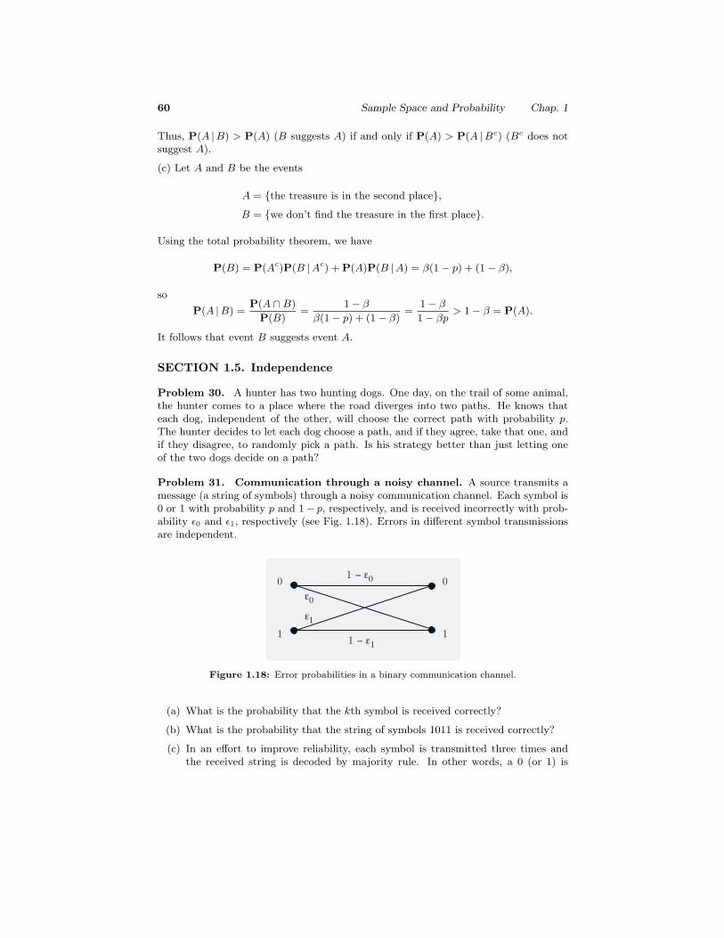
60 Sample Space and Probability Chap. 1
Thus, P(A |B) > P(A) (B suggests A) if and only if P(A) > P(A |Bc) (Bc does notsuggest A).
(c) Let A and B be the events
A = {the treasure is in the second place},B = {we don’t find the treasure in the first place}.
Using the total probability theorem, we have
P(B) = P(Ac)P(B |Ac) + P(A)P(B |A) = β(1 − p) + (1 − β),
so
P(A |B) =P(A ∩ B)
P(B)=
1 − β
β(1 − p) + (1 − β)=
1 − β
1 − βp> 1 − β = P(A).
It follows that event B suggests event A.
SECTION 1.5. Independence
Problem 30. A hunter has two hunting dogs. One day, on the trail of some animal,the hunter comes to a place where the road diverges into two paths. He knows thateach dog, independent of the other, will choose the correct path with probability p.The hunter decides to let each dog choose a path, and if they agree, take that one, andif they disagree, to randomly pick a path. Is his strategy better than just letting oneof the two dogs decide on a path?
Problem 31. Communication through a noisy channel. A source transmits amessage (a string of symbols) through a noisy communication channel. Each symbol is0 or 1 with probability p and 1− p, respectively, and is received incorrectly with prob-ability ε0 and ε1, respectively (see Fig. 1.18). Errors in different symbol transmissionsare independent.
ε1
1 1
0 0
ε0
1 − ε0
1 − ε1
Figure 1.18: Error probabilities in a binary communication channel.
(a) What is the probability that the kth symbol is received correctly?
(b) What is the probability that the string of symbols 1011 is received correctly?
(c) In an effort to improve reliability, each symbol is transmitted three times andthe received string is decoded by majority rule. In other words, a 0 (or 1) is
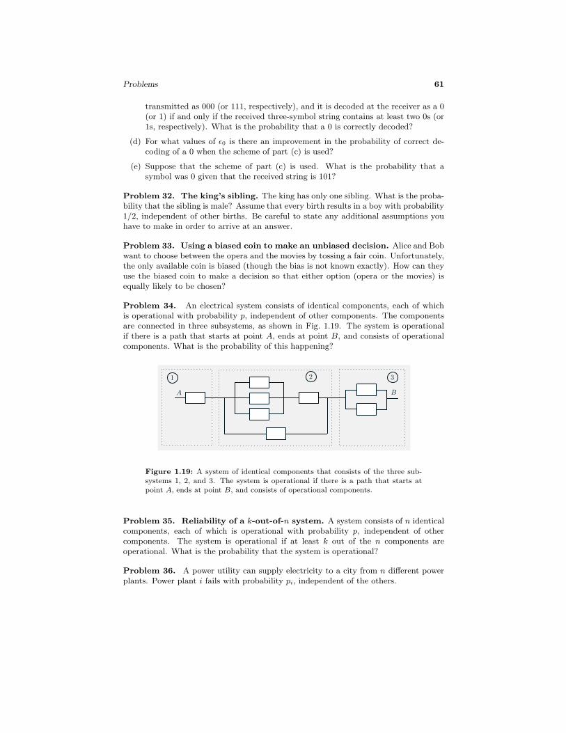
Problems 61
transmitted as 000 (or 111, respectively), and it is decoded at the receiver as a 0(or 1) if and only if the received three-symbol string contains at least two 0s (or1s, respectively). What is the probability that a 0 is correctly decoded?
(d) For what values of ε0 is there an improvement in the probability of correct de-coding of a 0 when the scheme of part (c) is used?
(e) Suppose that the scheme of part (c) is used. What is the probability that asymbol was 0 given that the received string is 101?
Problem 32. The king’s sibling. The king has only one sibling. What is the proba-bility that the sibling is male? Assume that every birth results in a boy with probability1/2, independent of other births. Be careful to state any additional assumptions youhave to make in order to arrive at an answer.
Problem 33. Using a biased coin to make an unbiased decision. Alice and Bobwant to choose between the opera and the movies by tossing a fair coin. Unfortunately,the only available coin is biased (though the bias is not known exactly). How can theyuse the biased coin to make a decision so that either option (opera or the movies) isequally likely to be chosen?
Problem 34. An electrical system consists of identical components, each of whichis operational with probability p, independent of other components. The componentsare connected in three subsystems, as shown in Fig. 1.19. The system is operationalif there is a path that starts at point A, ends at point B, and consists of operationalcomponents. What is the probability of this happening?
321
A B
Figure 1.19: A system of identical components that consists of the three sub-systems 1, 2, and 3. The system is operational if there is a path that starts atpoint A, ends at point B, and consists of operational components.
Problem 35. Reliability of a k-out-of-n system. A system consists of n identicalcomponents, each of which is operational with probability p, independent of othercomponents. The system is operational if at least k out of the n components areoperational. What is the probability that the system is operational?
Problem 36. A power utility can supply electricity to a city from n different powerplants. Power plant i fails with probability pi, independent of the others.
62 Sample Space and Probability Chap. 1
(a) Suppose that any one plant can produce enough electricity to supply the entirecity. What is the probability that the city will experience a black-out?
(b) Suppose that two power plants are necessary to keep the city from a black-out.Find the probability that the city will experience a black-out.
Problem 37. A cellular phone system services a population of n1 “voice users” (thosewho occasionally need a voice connection) and n2 “data users” (those who occasionallyneed a data connection). We estimate that at a given time, each user will need to beconnected to the system with probability p1 (for voice users) or p2 (for data users),independent of other users. The data rate for a voice user is r1 bits/sec and for a datauser is r2 bits/sec. The cellular system has a total capacity of c bits/sec. What is theprobability that more users want to use the system than the system can accommodate?
Problem 38. The problem of points. Telis and Wendy play a round of golf (18holes) for a $10 stake, and their probabilities of winning on any one hole are p and1 − p, respectively, independent of their results in other holes. At the end of 10 holes,with the score 4 to 6 in favor of Wendy, Telis receives an urgent call and has to reportback to work. They decide to split the stake in proportion to their probabilities ofwinning had they completed the round, as follows. If pT and pW are the conditionalprobabilities that Telis and Wendy, respectively, are ahead in the score after 18 holesgiven the 4-6 score after 10 holes, then Telis should get a fraction pT /(pT + pW ) of thestake, and Wendy should get the remaining pW /(pT + pW ). How much money shouldTelis get? Note: This is an example of the, so-called, problem of points, which playedan important historical role in the development of probability theory. The problemwas posed by Chevalier de Mere in the 17th century to Pascal, who introduced theidea that the stake of an interrupted game should be divided in proportion to theplayers’ conditional probabilities of winning given the state of the game at the time ofinterruption. Pascal worked out some special cases and through a correspondence withFermat, stimulated much thinking and several probability-related investigations.
Problem 39. A particular class has had a history of low attendance. The annoyedprofessor decides that she will not lecture unless at least k of the n students enrolledin the class are present. Each student will independently show up with probabilitypg if the weather is good, and with probability pb if the weather is bad. Given theprobability of bad weather on a given day, obtain an expression for the probability thatthe professor will teach her class on that day.
Problem 40. Consider a coin that comes up heads with probability p and tails withprobability 1− p. Let qn be the probability that after n independent tosses, there havebeen an even number of heads. Derive a recursion that relates qn to qn−1, and solvethis recursion to establish the formula
qn =(1 + (1 − 2p)n
)/2.
Problem 41. Consider a game show with an infinite pool of contestants, whereat each round i, contestant i obtains a number by spinning a continuously calibratedwheel. The contestant with the smallest number thus far survives. Successive wheelspins are independent and we assume that there are no ties. Let N be the round atwhich contestant 1 is eliminated. For any positive integer n, find P(N = n).
Problems 63
Problem 42.* Gambler’s ruin. A gambler makes a sequence of independent bets.In each bet, he wins $1 with probability p, and loses $1 with probability 1−p. Initially,the gambler has $k, and plays until he either accumulates $n or has no money left.What is the probability that the gambler will end up with $n?
Solution. Let us denote by A the event that he ends up with $n, and by F the eventthat he wins the first bet. Denote also by wk the probability of event A, if he startswith $k. We apply the total probability theorem to obtain
wk = P(A |F )P(F ) + P(A |F c)P(F c) = pP(A |F ) + qP(A |F c), 0 < k < n,
where q = 1−p. By the independence of past and future bets, having won the first betis the same as if he were just starting now but with $(k+1), so that P(A |F ) = wk+1
and similarly P(A |F c) = wk−1. Thus, we have wk = pwk+1 + qwk−1, which can bewritten as
wk+1 − wk = r(wk − wk−1), 0 < k < n,
where r = q/p. We will solve for wk in terms of p and q using iteration, and theboundary values w0 = 0 and wn = 1.
We have wk+1 − wk = rk(w1 − w0), and since w0 = 0,
wk+1 = wk + rkw1 = wk−1 + rk−1w1 + rkw1 = w1 + rw1 + · · · + rkw1.
The sum in the right-hand side can be calculated separately for the two cases wherer = 1 (or p = q) and r �= 1 (or p �= q). We have
wk =
{1 − rk
1 − rw1, if p �= q,
kw1, if p = q.
Since wn = 1, we can solve for w1 and therefore for wk:
w1 =
⎧⎪⎨⎪⎩
1 − r
1 − rn, if p �= q,
1
n, if p = q,
so that
wk =
⎧⎪⎨⎪⎩
1 − rk
1 − rn, if p �= q,
k
n, if p = q.
Problem 43.* Let A and B be independent events. Use the definition of indepen-dence to prove the following:
(a) The events A and Bc are independent.
(b) The events Ac and Bc are independent.
Solution. (a) The event A is the union of the disjoint events A∩Bc and A∩B. Usingthe additivity axiom and the independence of A and B, we obtain
P(A) = P(A ∩ B) + P(A ∩ Bc) = P(A)P(B) + P(A ∩ Bc).
64 Sample Space and Probability Chap. 1
It follows thatP(A ∩ Bc) = P(A)
(1 − P(B)
)= P(A)P(Bc),
so A and Bc are independent.
(b) Apply the result of part (a) twice: first on A and B, then on Bc and A.
Problem 44.* Let A, B, and C be independent events, with P(C) > 0. Prove thatA and B are conditionally independent given C.
Solution. We have
P(A ∩ B |C) =P(A ∩ B ∩ C)
P(C)
=P(A)P(B)P(C)
P(C)
= P(A)P(B)
= P(A |C)P(B |C),
so A and B are conditionally independent given C. In the preceding calculation, thefirst equality uses the definition of conditional probabilities; the second uses the as-sumed independence; the fourth uses the independence of A from C, and of B from C.
Problem 45.* Assume that the events A1, A2, A3, A4 are independent and thatP(A3 ∩ A4) > 0. Show that
P(A1 ∪ A2 |A3 ∩ A4) = P(A1 ∪ A2).
Solution. We have
P(A1 |A3 ∩ A4) =P(A1 ∩ A3 ∩ A4)
P(A3 ∩ A4)=
P(A1)P(A3)P(A4)
P(A3)P(A4)= P(A1).
We similarly obtain P(A2 |A3 ∩A4) = P(A2) and P(A1 ∩A2 |A3 ∩A4) = P(A1 ∩A2),and finally,
P(A1 ∪ A2 |A3 ∩ A4) = P(A1 |A3 ∩ A4) + P(A2 |A3 ∩ A4) − P(A1 ∩ A2 |A3 ∩ A4)
= P(A1) + P(A2) − P(A1 ∩ A2)
= P(A1 ∪ A2).
Problem 46.* Laplace’s rule of succession. Consider m + 1 boxes with the kthbox containing k red balls and m − k white balls, where k ranges from 0 to m. Wechoose a box at random (all boxes are equally likely) and then choose a ball at randomfrom that box, n successive times (the ball drawn is replaced each time, and a new ballis selected independently). Suppose a red ball was drawn each of the n times. Whatis the probability that if we draw a ball one more time it will be red? Estimate thisprobability for large m.
Solution. We want to find the conditional probability P(E |Rn), where E is the eventof a red ball drawn at time n+1, and Rn is the event of a red ball drawn each of the npreceding times. Intuitively, the consistent draw of a red ball indicates that a box with
Problems 65
a high percentage of red balls was chosen, so we expect that P(E |Rn) is closer to 1than to 0. In fact, Laplace used this example to calculate the probability that the sunwill rise tomorrow given that it has risen for the preceding 5,000 years. (It is not clearhow serious Laplace was about this calculation, but the story is part of the folklore ofprobability theory.)
We have
P(E |Rn) =P(E ∩ Rn)
P(Rn),
and by using the total probability theorem, we obtain
P(Rn) =
m∑k=0
P(kth box chosen)(
k
m
)n
=1
m + 1
m∑k=0
(k
m
)n
,
P(E ∩ Rn) = P(Rn+1) =1
m + 1
m∑k=0
(k
m
)n+1
.
For large m, we can view P(Rn) as a piecewise constant approximation to an integral:
P(Rn) =1
m + 1
m∑k=0
(k
m
)n
≈ 1
(m + 1)mn
∫ m
0
xndx =1
(m + 1)mn· mn+1
n + 1≈ 1
n + 1.
Similarly,
P(E ∩ Rn) = P(Rn+1) ≈ 1
n + 2,
so that
P(E |Rn) ≈ n + 1
n + 2.
Thus, for large m, drawing a red ball one more time is almost certain when n is large.
Problem 47.* Binomial coefficient formula and the Pascal triangle.
(a) Use the definition of(
nk
)as the number of distinct n-toss sequences with k
heads, to derive the recursion suggested by the so called Pascal triangle, given inFig. 1.20.
(b) Use the recursion derived in part (a) and induction, to establish the formula
(n
k
)=
n!
k! (n − k)!.
Solution. (a) Note that n-toss sequences that contain k heads (for 0 < k < n) can beobtained in two ways:
(1) By starting with an (n−1)-toss sequence that contains k heads and adding a tailat the end. There are
(n−1
k
)different sequences of this type.
(2) By starting with an (n − 1)-toss sequence that contains k − 1 heads and addinga head at the end. There are
(n−1k−1
)different sequences of this type.

66 Sample Space and Probability Chap. 1
( )( )
( )
1
2
4
23
03
22
11
13
33
00
04
14
24
34
44
12
02
01
1 1
. . . . . . . .
4
1 1
1 1
1 1
3
6
3
. . . . . . . .
( )
( )
( ) ( )
( ) ( )
( )( ) ( )
( )( ) ( )
Figure 1.20: Sequential calculation method of the binomial coefficients using thePascal triangle. Each term
(nk
)in the triangular array on the left is computed
and placed in the triangular array on the right by adding its two neighbors in therow above it (except for the boundary terms with k = 0 or k = n, which are equalto 1).
Thus, (n
k
)=
⎧⎨⎩
(n − 1
k − 1
)+
(n − 1
k
), if k = 1, 2, . . . , n − 1,
1, if k = 0, n.
This is the formula corresponding to the Pascal triangle calculation, given in Fig. 1.20.
(b) We now use the recursion from part (a), to demonstrate the formula(n
k
)=
n!
k! (n − k)!,
by induction on n. Indeed, we have from the definition(10
)=
(11
)= 1, so for n = 1 the
above formula is seen to hold as long as we use the convention 0! = 1. If the formulaholds for each index up to n − 1, we have for k = 1, 2, . . . , n − 1,(
n
k
)=
(n − 1
k − 1
)+
(n − 1
k
)
=(n − 1)!
(k − 1)! (n − 1 − k + 1)!+
(n − 1)!
k! (n − 1 − k)!
=k
n· n!
k! (n − k)!+
n − k
n· n!
k! (n − k)!
=n!
k! (n − k)!,
and the induction is complete.
Problem 48.* The Borel-Cantelli lemma. Consider an infinite sequence of trials.The probability of success at the ith trial is some positive number pi. Let N be the
Problems 67
event that there is no success, and let I be the event that there is an infinite numberof successes.
(a) Assume that the trials are independent and that∑∞
i=1pi = ∞. Show that
P(N) = 0 and P(I) = 1.
(b) Assume that∑∞
i=1pi < ∞. Show that P(I) = 0.
Solution. (a) The event N is a subset of the event that there were no successes in thefirst n trials, so that
P(N) ≤n∏
i=1
(1 − pi).
Taking logarithms,
log P(N) ≤n∑
i=1
log(1 − pi) ≤n∑
i=1
(−pi).
Taking the limit as n tends to infinity, we obtain log P(N) = −∞, or P(N) = 0.Let now Ln be the event that there is a finite number of successes and that the
last success occurs at the nth trial. We use the already established result P(N) = 0,and apply it to the sequence of trials after trial n, to obtain P(Ln) = 0. The event Ic
(finite number of successes) is the union of the disjoint events Ln, n ≥ 1, and N , sothat
P(Ic) = P(N) +
∞∑n=1
P(Ln) = 0,
and P(I) = 1.
(b) Let Si be the event that the ith trial is a success. Fix some number n and for everyi > n, let Fi be the event that the first success after time n occurs at time i. Notethat Fi ⊂ Si. Finally, let An be the event that there is at least one success after timen. Note that I ⊂ An, because an infinite number of successes implies that there aresuccesses subsequent to time n. Furthermore, the event An is the union of the disjointevents Fi, i > n. Therefore,
P(I) ≤ P(An) = P
(∞⋃
i=n+1
Fi
)=
∞∑i=n+1
P(Fi) ≤∞∑
i=n+1
P(Si) =
∞∑i=n+1
pi.
We take the limit of both sides as n → ∞. Because of the assumption∑∞
i=1pi < ∞,
the right-hand side converges to zero. This implies that P(I) = 0.
SECTION 1.6. Counting
Problem 49. De Mere’s puzzle. A six-sided die is rolled three times independently.Which is more likely: a sum of 11 or a sum of 12? (This question was posed by theFrench nobleman de Mere to his friend Pascal in the 17th century.)
Problem 50. The birthday problem. Consider n people who are attending aparty. We assume that every person has an equal probability of being born on any day

68 Sample Space and Probability Chap. 1
during the year, independent of everyone else, and ignore the additional complicationpresented by leap years (i.e., assume that nobody is born on February 29). What isthe probability that each person has a distinct birthday?
Problem 51. An urn contains m red and n white balls.
(a) We draw two balls randomly and simultaneously. Describe the sample space andcalculate the probability that the selected balls are of different color, by usingtwo approaches: a counting approach based on the discrete uniform law, and asequential approach based on the multiplication rule.
(b) We roll a fair 3-sided die whose faces are labeled 1,2,3, and if k comes up, weremove k balls from the urn at random and put them aside. Describe the samplespace and calculate the probability that all of the balls drawn are red, using adivide-and-conquer approach and the total probability theorem.
Problem 52. We deal from a well-shuffled 52-card deck. Calculate the probabilitythat the 13th card is the first king to be dealt.
Problem 53. Ninety students, including Joe and Jane, are to be split into threeclasses of equal size, and this is to be done at random. What is the probability thatJoe and Jane end up in the same class?
Problem 54. Twenty distinct cars park in the same parking lot every day. Ten ofthese cars are US-made, while the other ten are foreign-made. The parking lot hasexactly twenty spaces, all in a row, so the cars park side by side. However, the drivershave varying schedules, so the position any car might take on a certain day is random.
(a) In how many different ways can the cars line up?
(b) What is the probability that on a given day, the cars will park in such a waythat they alternate (no two US-made are adjacent and no two foreign-made areadjacent)?
Problem 55. Eight rooks are placed in distinct squares of an 8× 8 chessboard, withall possible placements being equally likely. Find the probability that all the rooks aresafe from one another, i.e., that there is no row or column with more than one rook.
Problem 56. An academic department offers 8 lower level courses: {L1, L2, . . . , L8}and 10 higher level courses: {H1, H2, . . . , H10}. A valid curriculum consists of 4 lowerlevel courses, and 3 higher level courses.
(a) How many different curricula are possible?
(b) Suppose that {H1, . . . , H5} have L1 as a prerequisite, and {H6, . . . H10} have L2
and L3 as prerequisites, i.e., any curricula which involve, say, one of {H1, . . . , H5}must also include L1. How many different curricula are there?
Problem 57. How many 6-word sentences can be made using each of the 26 lettersof the alphabet exactly once? A word is defined as a nonempty (possibly jibberish)sequence of letters.
Problems 69
Problem 58. We draw the top 7 cards from a well-shuffled standard 52-card deck.Find the probability that:
(a) The 7 cards include exactly 3 aces.
(b) The 7 cards include exactly 2 kings.
(c) The probability that the 7 cards include exactly 3 aces, or exactly 2 kings, orboth.
Problem 59. A parking lot contains 100 cars, k of which happen to be lemons. Weselect m of these cars at random and take them for a test drive. Find the probabilitythat n of the cars tested turn out to be lemons.
Problem 60. A well-shuffled 52-card deck is dealt to 4 players. Find the probabilitythat each of the players gets an ace.
Problem 61.* Hypergeometric probabilities. An urn contains n balls, out ofwhich m are red. We select k of the balls at random, without replacement (i.e., selectedballs are not put back into the urn before the next selection). What is the probabilitythat i of the selected balls are red?
Solution. The sample space consists of the(
nk
)different ways that we can select k out
of the available balls. For the event of interest to occur, we have to select i out of them red balls, which can be done in
(mi
)ways, and also select k− i out of the n−m balls
that are not red, which can be done in(
n−mk−i
)ways. Therefore, the desired probability
is (m
i
)(n − m
k − i
)(
n
k
) ,
for i ≥ 0 satisfying i ≤ m, i ≤ k, and k − i ≤ n − m. For all other i, the probability iszero.
Problem 62.* Correcting the number of permutations for indistinguishableobjects. When permuting n objects, some of which are indistinguishable, differentpermutations may lead to indistinguishable object sequences, so the number of distin-guishable object sequences is less than n!. For example, there are six permutations ofthe letters A, B, and C:
ABC, ACB, BAC, BCA, CAB, CBA,
but only three distinguishable sequences that can be formed using the letters A, D,and D:
ADD, DAD, DDA.
(a) Suppose that k out of the n objects are indistinguishable. Show that the numberof distinguishable object sequences is n!/k!.
(b) Suppose that we have r types of indistinguishable objects, and for each i, ki
objects of type i. Show that the number of distinguishable object sequences is
n!
k1! k2! · · · kr!.
70 Sample Space and Probability Chap. 1
Solution. (a) Each one of the n! permutations corresponds to k! duplicates which areobtained by permuting the k indistinguishable objects. Thus, the n! permutations canbe grouped into n!/k! groups of k! indistinguishable permutations that result in thesame object sequence. Therefore, the number of distinguishable object sequences isn!/k!. For example, the three letters A, D, and D give the 3! = 6 permutations
ADD, ADD, DAD, DDA, DAD, DDA,
obtained by replacing B and C by D in the permutations of A, B, and C given earlier.However, these 6 permutations can be divided into the n!/k! = 3!/2! = 3 groups
{ADD, ADD}, {DAD, DAD}, {DDA, DDA},
each having k! = 2! = 2 indistinguishable permutations.
(b) One solution is to extend the argument in (a) above: for each object type i, there areki! indistinguishable permutations of the ki objects. Hence, each permutation belongsto a group of k1! k2! · · · kr! indistinguishable permutations, all of which yield the sameobject sequence.
An alternative argument goes as follows. Choosing a distinguishable object se-quence is the same as starting with n slots and for each i, choosing the ki slots to beoccupied by objects of type i. This is the same as partitioning the set {1, . . . , n} intogroups of size k1, . . . , kr, and the number of such partitions is given by the multinomialcoefficient.