Department of MathematicsGeometry of Manifolds, 18.966

Spring 2005 Lecture Notes

1 The Levi-Civita Connection and its curva-

ture

In this lecture we introduce the most important connection. This is theLevi-Civita connection in the tangent bundle of a Riemannian manifold.

1.1 The Einstein summation convention and the RicciCalculus

When dealing with tensors on a manifold it is convient to use the followingconventions. When we choose a local frame for the tangent bundle we writee1, . . . en for this basis. We always index bases of the tangent bundle withindices down. We write then a typical tangent vector

X =n∑

i=1

X iei.

Einstein’s convention says that when we see indices both up and down weassume that we are summing over them so he would write

X = X iei

while a one form would be written as

θ = aiei

where ei is the dual co-frame field. For example when we have coordinatesx1, x2, . . . , xn then we get a basis for the tangent bundle

∂/∂x1, . . . , ∂/∂xn

1

More generally a typical tensor would be written as

T = T ijk

lei ⊗ ej ⊗ ek ⊗ el

Note that in general unless the tensor has some extra symmetries the orderof the indices matters. The lower indices indicate that under a change offrame fi = Ci

jej a lower index changes the same way and is called covariantwhile an upper index changes by the inverse matrix. For example the dualcoframe field to the fi, called f i is given by

f i = Dije

j

where Dij is the inverse matrix to Cj

i (so that DijC

jk = δi

k.) The compo-nents of the tensor T above in the fi basis are thus

T ijk

l = T i′j′k′

l′Dii′C

j′jC

k′kD

ll′

Notice that of course summing over a repeated upper and lower index resultsin a quantity that is independent of any choices.

Given a vector bundle over our manifold which is not the tangent bundleor tensors on the tangent bundle we use a distinct set of indices to indicatetensors with values on that bundle. If V → M is a vector bundle of rank kwith a local frame vα, 1 ≤ α ≤ r we would write

s = cαi vα ⊗ dxi

for a typical section of the bundle T ∗M ⊗ VGiven a ∇ connection in V we write

∇s = sα;idxi ⊗ vα.

That is we think ∇s as a section of T ∗M ⊗ V as opposed to the possiblymore natural V ⊗T ∗M . Or more concretely the semi-colon is also indicatingthat the indices following the semi-colon are to really be thought of commingfirst and the opposite order. Our convention here is designed to be moreconsistent with the mathematical literature. In the physics literature forexample “Graviation” by Misner, Throne and Wheeler. So for a connectionin the tangent bundle if we have a vector field with components X i we havewrite X i

,j for the components of its covariant derivative. The Christoffel

2

symbols of a connection are the components of the covariant derivatives ofthe basis vectors:

∇eivα = Γi

αβvβ.

Then we can write more explicitly

sα;i = eis

α + Γiα

βsβ

One often uses the short hand

eisα = sα

,i

so thatsα

;i = sα,i + Γi

αβsβ

1.2 The low brow approach to the Levi-Civita connec-tion

The Levi-Civita connection is characterized by two properties. First that itis metric compatible, i.e. that

X〈Y, Z〉 = 〈∇XY, Z〉+ 〈Y,∇Y Z〉

or equivalently that parallel transport is an isometry. For a connnection inthe tangent bundle there is another property to ask for called torsion free.The torsion of a connection in the tangent bundle is the tensor

T (X, Y ) = ∇XY −∇Y X − [X, Y ]

and the torsion free condition means that this tensor is indentically zero.Since the coordinate vector field commute the expression for the componentsof torsion in terms of a coordinate frame is

Tikj = Γi

kj − Γj

ki.

The Let ∇ a torsion free connection metric compatible connection.

Lemma 1.1.

Γikj =

1

2gkl(gjl,i + gil,j − gij,l)

3

Proof. Notice that there are n3 distinct functions involved in defining a con-nection. Recall that the torsion free condition implies n2(n− 1)/2 relationsamongst these functions:

Γkij = Γk

ji. (1)

The metric compatibility implies n2(n + 1)/2 relations amongst these func-tions:

gij,l = 〈∇ ∂

∂xl

∂

∂xi,

∂

∂xj〉+ 〈 ∂

∂xi,∇ ∂

∂xl

∂

∂xj〉

= gkjΓkli + gikΓ

klj.

Hence using equation 1

gjl,i + gil,j − gij,l = gklΓkij + gjkΓ

kil

+gkjΓkji + gikΓ

kjl

−gkjΓkli − gikΓ

klj

= 2gklΓkij

and the result follows.

1.3 The method of moving frames

We will now redo the existence of the Levi-Civita connection from the pointof view of the induced connection on the cotangent bundle. This methodis more compuationally effective. A connection ∇ in the tangent bundleinduces a connection ∇∗ in the cotangent bundle by the requiring

Xθ(Y ) = ∇∗Xθ(Y ) + θ(∇XY ).

After this section we’ll drop the ∗ from the notation nice the meaning willbe clear from context. To justify this definition think about the conditionthat the parallet transport for the two connections is equivalent.

Thus if Γkij are the Christoffel symbols for ∇ we have

∇∗∂

∂xidxk = −Γk

ijdxj.

4

Lemma 1.2. The condition that ∇ is torsion free is equivalent to the con-dition that for any one-form α we have

dα(X, Y ) = ∇∗Xα(Y )−∇∗Y α(X).

Proof. To see this notice

∇∗Xα(Y )−∇∗Y α(X)− dα(X, Y )

= Xα(Y )− α(∇XY )− Y α(X) + α(∇Y X)

− (Xα(Y )− Y α(X)− α([X, Y ]))

= α(−∇XY +∇XY + [X, Y ]).

A crucial step is to use an orthonormal frame e1, . . . , en and dual coframee1, e2, . . . , en then we have the Christoffel symbols for the connection

∇eiej = Γk

ijek

∇∗eiek = −Γk

ijej

Thus connection matrix for the dual connection is

∇ek = −Γkije

i ⊗ ej

The torsion free condition then implies

dek = −Γkije

i ∧ ej

From the equationei〈ej, ek〉 = 0

we derive that if ∇ is metric compatible then

Γkij = −Γj

ik.

Let’s prove, from this point of view, the basic uniqueness theorem the Levi-Civita connection.

Lemma 1.3. There is a unique torsion free metric compatible connection.

5

Proof. Suppose that ∇′ is another metric compatible torsion free connec-tion with connection matrix ηk

j and dual connection matrix −ηkj . Write the

difference as−θk

j + ηkj = fk

ijei.

Then the torsion free condition implies

0 = fkije

i ∧ ej

so that fkij = fk

ji. Metric compatible implies that fkij = −f j

ik and so

fkij = −f j

ik = −f jki = f i

kj = f ijk = −fk

ji

and so fkij = 0.

To finish this discussion we need to see that we can solve the equation

dek = −θkj ∧ ej.

Where θkj = Γk

ijei and Γk

ij = −Γjik so there are n×n(n−1)/2 unknowns. This

is n equations for two forms hence is n×n(n−1)/2 equations. We have seenthat the solution is unique and hence exists.

To make this a useful method for computing we need to understand moreconcretely how to compute with the answer. Suppose that

dek = Akije

i ∧ ej.

When we do calculations we are naturally get these Akij with Ak

ij = −Akji. To

find the Christoffel symbols we simply set

Γkij = −Ak

ij + Ajik + Ai

jk.

Note that with this definition

Γkij = −Γj

ik.

Since Ajik + Ai

jk is symmetric in i and j we still have

dek = Γkije

i ∧ ej.

For example in hyperbolic space

Hn+1

6

with the metric

ds2 =1

x20

((dx0)2 + (dx1)2) + . . . + (dxn)2)

we have

ei =dxi

x0

and hence de0 = 0 while for i > 0 we have

dei = −dx0 ∧ dxi

(x0)2= −e0ei.

So for i > 0

Ai0i =

1

2= −Ai

i0.

Thusθi0 = (Ai

j0 − A0ji − Aj

i0)ej = −ei

and θij = 0 if i, j > 0.

1.4 Working on the frame bundle

The calculations above are straighforward but it is natural to look for a homefor them. The bundle of orthonormal frames provides the right framework.After all in particular in the method of moving frames our choice was a localorthonormal frame field. A better way to view what is going on is to workwith all frames simulatenously. The primordial object is the bunlde of frames(bases) of the tangent bundle π : Fr(M) → M .

Given a frame f1, . . . , fn and an matrix aij we get a new orthonormalframe f ′i =

∑nj=1 aijfj or a little more clearly we think of the orginal frame

f = f1, . . . , fn as giving an isomorphism

f : Rn → TxM.

Then an isomorphism of a : Rn → Rn we get a new frame

f a : Rn → TxM.

This make Fr(M) into a principal Gl(n) bundle. That is there is a map

Fr(M)×Gl(n) → Fr(M)

7

so that(fA)B = f(AB).

Each orbit of the action is precisely one fiber of the projection and the actionis effective (fA = f =⇒ A = 1). Informally it is a bundle of groups wherethe transition functions act by left multiplicition on the group leaving theright action to act on the resulting bundle.

A connection gives rise to an Gl(n)-invariant horizontal subbundle of thetangent bundle of Fr(M). By this we mean a subbundle H ⊂ TFr(M) so thatπ∗|H : H → π∗TM is an isomorphism and so that for all a ∈ Gl(n) we have(Ra)∗H = H. The horizontal bundle associated to a connection is the lift ofthe tangent space given by the connection.

There is an exact sequence

0 → V TFr(M) → TFr(M) → π∗(TM) → 0.

Here V TFr(M) denotes the “vertical tangent bundle” to FrOr(M) i.e. thekernel of dπ. The vertical tangent bundle is trivial and each fiber is isomor-phic to the Lie algebra of Gl(n) as follows. Let A be a matrix and considerthe path e exp(tA). The derivative of the path at t = 0 defines a map

ιe : gl(n) → V TeFr(M).

We can thus rewrite this exact sequence as

0 → P × gl → TFr(M) → π∗(TM) → 0.

A connection is then a splitting of this exact sequence

0 → P × gln←→ TFr(M) → π∗(TM) → 0.

Let us work this out explictly. Given a connection in a vector bundle ifwe choose local coordinates xi in the base and a local frame e = (eα). Theframe e gives us a local trivialization so the principal bundle becomes

U ×Gln

We get Christoffel symbols

∇ ∂

∂xieα = Γβ

iαeβ.

8

So given a curve γ(t) = (x1(t), x2(t), . . . , xn(t)) its parallel lift means findingcα(t) so that

∂cα

∂t+

∂xi

∂tΓα

iβcβ = 0.

In particular if γ(t) = (0, . . . , t . . . , 0) and if the initial condition is one of thebasis vector eβ

∂cα

∂t(0) + Γα

iβ(0, . . . , 0) = 0.

From this we deduce that the horizontal space at the given orthonormalframe e is spanned by the n vectors

(∂

∂xi,−Γβ

iα). (2)

Here we are writing the tangent space of Gln at the identity as Mn the spaceof n× n-matrices.

There is a distinguished gln-valued one form on Gln namely the one formwhich identifies the tangent space at A with the tangent space at the identity.This one form, called the Mauer-Cartan form at a matrix A can be written

ωMC |A = A−1dA

In other words the Mauer-Cartan form sends ξ ∈ TAGln to A−1ξ ∈ TIGln.The vectors (2) are in the kernel of the gln-valued one form

θe = ωMC + dxiΓβiα

Notice that if we change frame so that e = eg where g : U → Gln. Thismeans that

eα = gβαeα

then the Chirstoffel symbols change by

Γβiα = (g−1)γ

α

∂gβγ

∂xi(g−1)β

γ + Γδiγg

δα

while the Mauer-Cartan form changes by

ωMC |Bg = g−1(B−1dB)g = g−1ωMC |Bg + g−1dg

If we change frame i.e. we consider the map U ×Gln → U ×Gln given by

g : (x, A) 7→ (x, Ag(x))

9

and we pull backNote that if γ(t) is the horizontal lift at a frame e of γ then γ(t)A is the

horizontal lift of γ at eA. This implies that right translation preserves thehorizontal space of the connection and in particular that

θeA = R∗Aθe.

Note that that a section of the tangent bundle is given as a map

X : Fr(M) → Rn

with the equivariance property

X(fA) = A−1X(f)

Given a connection we canThis bundle carries a tautological Rn-valued one form

θ : TFr(M) → Rn.

It is defined as follows. Given a tangent vector v to TFr(M) at a frame f wecan project v to TM and expand it in terms of f

θ(v) = f−1(π∗(v)).

The tautological one form gives a geometric interpretation of torsion. Underthe action of Gl(n) this one-form transforms by

(Ra)∗θ = a−1θ

Since θ has values in vector spaceTo this end we set π : FrOr(M) → M to be the bundle of orthonormal

frames on M . This is principal O(n) bundle. Given a frame e1, . . . , en andan orthogonal matrix aij we get a new orthonormal frame fi =

∑nj=1 aijej or

a little more clearly we think of the orginal frame e = e1, . . . , en as givingan isometry

e : Rn → TxM.

Then an isometry of a : Rn → Rn we get a new frame

e a : Rn → TxM.

10

Given a connection its parallel transport gives rise to a lift through anypoint e of the total space of each path in a the base passing through π(e).Taking derivatives we get a lifting of the TeM to TeFrOr(M) for each e.Notice that the tangent bundle of FrOr(M) is trivial. As have seen thatGiven a tangent vector ei in the base its lift to FrOr(M) at e is e

Consider more generally a principal G bundle P → M where G is a Liegroup. We will always think of G as acting on P on the right. The verticaltangent bundle of any principal bundle is alway trival and indeed each fibercan be identified with the Lie Algebra of the structure group. To see this letξ ∈ g be an element of the structure group which we always identify withleft invariant vector fields on G.

1.5 A first pass at the curvature

The curvature of the connection is

R(X, Y )Z = ∇X∇Y Z −∇Y∇XZ −∇[X,Y ]Z.

The coordinate expression of R is

R(∂

∂xi,

∂

∂xj)

∂

∂xk= Rijk

l ∂

∂xl.

In the trivialization given by our orthonormal frame the curvature of theLevi-Civita connection has the form

Ωlk = dθl

k + θlm ∧ θm

k .

This is related to the curvature tensor R as follows. Defining as above

Rijkl = 〈R(ei, ej)ek, el〉.

then we have

Lemma 1.4.

[Ωlk] = [

1

2Rijkle

i ∧ ej].

11

Proof. Since both side of the equation are independent of the frame it sufficeto work in normal coordinates about x and compute at x.

Ωlk(ei, ej) = dθl

k(ei, ej) + θlm ∧ θm

k (ei, ej)

= eiθlk(ej)− ejθ

lk(ei)

= eiΓljk − ejΓ

lik

which is Rijkl at x.

1.6 Symmetries of the curvature tensor

We defined the (3, 1)-Riemann curvature tensor to be

R(X, Y )Z = ∇X∇Y Z −∇Y∇XZ −∇[X,Y ]Z.

where ∇ is the Levi-Civita connection of the metric g or 〈, 〉. We also definethe (4, 0) curvature tensor

R(X,Y, Z, W ) = 〈R(X, Y )Z,W 〉.

The curvature has the following symmetries

Proposition 1.5. 1. R(X, Y, Z, W ) = −R(Y, X, Z, W )

2. R(X, Y, Z, W ) = −R(X, Y, W, Z)

3. R(X, Y, Z, W ) + R(Y, Z,X, W ) + R(Z,X, Y, W ) = 0

4. R(X, Y, Z, W ) = R(Z,W, X, Y )

Proof. The first item is obvious. The second is also obvious from our pointof view. The third follows from Jacobi identity. To see the fourth notice that

0 = R(X, Y, Z, W ) + R(Y, Z,X, W ) + R(Z,X, Y, W )

+R(Y,X, W, Z) + R(W, Y, X, Z) + R(X, W, Y, Z)

−(R(Z, Y,W,X) + R(Y,W, Z,X) + R(W, Z, Y,X))

−(R(X, Z, W, Y ) + R(Z,W,X, Y ) + R(W, X,Z, Y ))

= 2(R(X, Y, Z, W )−R(Z,W,X, Y ))

12

There is another differential equation obeyed by the curvature called thesecond Bianchi identity.

Lemma 1.6.dΩl

k + θlm ∧ Ωm

k − Ωmk ∧ θl

m = 0

Proof. Taking d of the formula Ωlk = dθl

k + θlm ∧ θm

k yields

dΩlk = dθl

m ∧ θmk − θl

m ∧ dθmk

= (Ωlm − θl

n ∧ θnm) ∧ θm

k − θlm ∧ (Ωm

k − θmn ∧ θn

k )

= Ωlm ∧ θm

k − θlm ∧ Ωm

k

In terms of the curvature tensor R the second Bianchi identity takes theform

(∇XR)(Y, Z)W + (∇Y R)(Z,X)W + (∇ZR)(X, Y )W = 0

1.7 Sectional curvature

The sectional curvature is the function on the Grassmanian of two planesgiven by

K(Π) = R(e, f, e, f)

where (e, f) is an orthonormal frame for Π. More generally if X, Y span Πthen

K(Π) =R(X, Y, X, Y )

|X|2|Y |2 − 〈X,Y 〉2

The sectional curvature determines the full curvature.

∂2

∂s∂t(R(X+tZ, Y +sW, X+tZ, Y +sW )−R(X+tW, Y +sZ,X+tW, Y +sZ)) = R(X, Y, Z, W )

In particular if K is a constant on the fibers of the Grassman bundle wehave

R(

13

1.8 Lie groups

A Lie group is a differentiable manifold and a group for which the grouplaws are differentiable. If G is a Lie group then for any g ∈ G we havediffeomorphisms

Lg, Rg : G → G

given by left and right multiplication respectively. Thus

(Lg)∗TeG → TgG

is an isomorphism and we can trivialize the tangent bundle of G. The formaldefinition of the Lie algebra of a Lie group is to use this isomorphism toidentify the tangent space at the identity with the left-invariant vector fields.

Definition 1.7. A one-parameter subgroup is a map

γ : R → G

so that γ(t + s) = γ(t)γ(s).

Every ξ ∈ g is tangent to a one pararmeter subgroup. To see this letFt : U ⊂ R × G → G be the flow for the vector field ξ where U is define sothat for each g ∈ G U ∩ R× g is the maximal interval of definition of theflow. First of all notice that since ξ is left invariant we have Lg F is alsothe flow for ξ from which it follows easily that U = R×G and that

Lg F (t, h) = F (t, gh) (3)

The flow has the semi-group property,

F (t + s, g) = F (t, F (s, g)) (4)

so if g = F (t, e) then

γ(t + s) = F (t + s, e) = F (s, F (t, e)) = F (s, ge) = gF (s, e) = γ(t)γ(s).

Proposition 1.8. Every compact Lie groups admits a bi-invariant metric.

Proposition 1.9. Let 〈, 〉 be a bi-invariant metric. Then for all left-invariantvector fieldsX, Y, Z we have

1. 〈[X, Y ], Z〉 = 〈X, [Y, Z]〉.

14

2. ∇XY = 12[X, Y ].

3. R(X, Y )Z = −14[[X,Y ], Z]

4. R(X, Y, Z, W ) = −14〈[X,Y ], [Z,W ]〉.

Proof. For the third item we compute:

R(X, Y )Z =1

4[X, [Y, Z]]− 1

4[Y, [X,Z]]− 1

2[[X, Y ], Z]

= −1

4[[X, Y ], Z]

The fourth formula follows immediately from this.

1.9 The curvature of a submanifold of a Riemannianmanifold

Let N ⊂ M be a submanifold. If M has a Riemannian metric then there isan induced Riemannian metric on N Let ν denote the normal bundle of Nin M¿ Then we can define the so called second fundamental form

II : TN × TN → ν.

byII(X, Y ) = Πν(∇XY ).

Lemma 1.10. II is tensorial and

II(X, Y ) = II(Y,X).

Proof. The first claim follows from the second so consider the

II(X, Y ) = Πν(∇XY )

= Πν(∇Y X + [X, Y ])

= Πν(∇Y X)

= II(Y, X).

.

15

For example if M = Rn+1 and N = Sn then

II(X, Y ) = 〈X, Y 〉.

Also notice that there is the following nice formula

Lemma 1.11. If ν is a normal vector field to N and X and Y are tangentthen:

〈∇Xν, Y 〉 = −〈ν, II(X, Y )〉

The second fundamental form determines the curvature of N is terms ofthe curvature of M .

Proposition 1.12. (The Gauss equations) For vector fields X, Y, Z tangentN we have:

RN(X, Y, W, Z) = RM(X, Y, Z, W )−〈II(X, Z), II(Y, W )〉+〈II(X, W ), II(Y, Z)〉

Proof. Suppose without loss of generality that X, Y, Z, W are vectors field onM which are tangent along N and that X and Y commute. Then we have

〈∇MX∇M

Y Z,W 〉 = 〈∇MX (∇N

Y Z + II(Y, Z), W 〉= 〈∇N

X∇NY Z + II(X,∇N

Y Z) +∇MX II(Y, Z), W 〉

= 〈∇NX∇N

Y ZW 〉 − 〈II(Y, Z), II(X,W )〉.

and hence

RN(X, Y, W, Z) = RM(X, Y, Z, W )−〈II(X, Z), II(Y, W )〉+〈II(X, W ), II(Y, Z)〉

Thus the curvature of Sn is

R(X, Y, Z, W ) = −〈X, Z〉〈Y, W 〉+ 〈X, W 〉〈Y, Z〉.

16

1.10 Semi-Riemannian manifolds.

So far nothing we have done really required the inner product on the tangentspace to be definite merely non-degenerate. As an example lets compute thecurvature of hyperbolic space.

Let Hn be the component of the hyperboloid

c = −x20 + x2

1 + . . . x2n = −1

containing (1, 0, 0, . . . , 0). Consider the Rn+1 with the Lorentz inner product.

m = −dx20 + dx2

1 + . . . dx2n.

Then1

2dc = −dx0 + dx1 + . . . + dxn

so the normal vector using m to Hn is still

n = (x0, x1, . . . , xn).

and soII(X, Y ) = −m(X, Y )n

and som(X, Z)m(Y,W )−m(X, W )m(Y, Z)

exactly the opposite of the sphere.

1.11 The decomposition of space of curvature tensorsinto irreducible representations of the orthogonalgroup

Let R denote the sub representation of Rn ⊗ Rn ⊗ Rn ⊗ Rn consisting of

1.12 The behavior of the curvature under conformalchange of metric.

Metrics g and g are said to be conformal if there is a function σ so that

g = e2σg

17

We will investgate how the various curvatures change conformal changeof metric. We will write 〈, 〉 for the g inner product and hence e2σ〈, 〉 denotesthe g-inner product.

Lemma 1.13. The Levi-Civita connections are related as follows:

∇XY = ∇XY + (Xσ)Y + (Y σ)X − 〈X, Y 〉∇σ (5)

Proof. Recall that the Levi-Civita connection ∇ is determined be the equa-tion

〈∇XY, Z〉 =1

2(X〈Y, Z〉+Y 〈X, Z〉−Z〈X,Y 〉+〈[X, Z], Y 〉+〈[Y, Z], X〉−〈[X,Y ], Z〉)

and so ∇ is determined by

e2σ〈∇XY, Z〉 =1

2(Xe2σ〈Y, Z〉+ Y e2σ〈X, Z〉 − Ze2σ〈X, Y 〉+

e2σ(〈[X, Z], Y 〉+ 〈[Y, Z], X〉 − 〈[X, Y ], Z〉))= e2σ(

1

2(X〈Y, Z〉+ Y 〈X, Z〉 − Z〈X, Y 〉

〈[X,Z], Y 〉+ 〈[Y, Z], X〉 − 〈[X, Y ], Z〉)= e2σ((Xσ)〈Y, Z〉+ (Y σ)〈X, Z〉 − (Zσ)〈X, Y 〉)

e2σ〈∇XY, Z〉

and so

〈∇XY, Z〉 = 〈∇XY, Z〉+ (Xσ)〈Y, Z〉+ (Y σ)〈X, Z〉 − 〈X, Y 〉〈∇σ, Z〉)

as required.

A long tedious calculation shows that

R(X,Y )Z = R(X, Y )Z +∇dσ(X, Z)Y −∇dσ(Y, Z)X − 〈Y, Z〉∇X∇σ + 〈X, Z〉∇Y∇σ

+ (Y σ)(Zσ)Z − (Xσ)(Zσ)Y − (Y σ)〈X, Z〉∇σ + (Xσ)〈Y, Z〉∇σ

− 〈Y, Z〉|∇σ|2X + 〈X,Z〉|∇σ|2Y

18

which can be rewritten as

R4,0 = e2σ(R4,0 + g ./ (∇dσ − dσ ⊗ dσ +

1

2|∇σ|2g)

)From which we glean

W 4,0 = e2σW 4,0

or that the (3,1)-Weyl curvature is conformally invariant. Notice then thatthe Weyl curvature is an obstruction to a metric being locally conformallyequivalent to the standard flat metric.

We can derive the behavior of the Ricci curvature Ric and the scalarcurvature s under conformal change of metric. Let cg denote the Ricci con-traction for the metric g. If e1 . . . , en is a local orthonormal frame then

cg(R)(ej, ek) =n∑

i=1

R(ej, ei, ek, ei)

so thatRic = −cg(R)

We will need the following.

Lemma 1.14. For all h ∈ Sym2(T ∗X) we have

cg(h ./ g) = trg(h) + (n− 2)h

Proof. A tedious calculation with indices.

Lemma 1.15. If g = e2σg then we have

Ric = Ric + (∆σ + (n− 2)|∇σ|2)g + (n− 2)(∇dσ − dσ dσ) (6)

ands = e−2σ(s + 2(n− 1)∆σ + (n− 1)(n− 2)|∇σ|2) (7)

19

1.13 Geodesics and curvature

Let γ : (a, b) → X be a smooth path. The energy of γ is

E(γ) =1

2

∫ b

a

|γ∗(∂

∂t)|2dt

and the length is

L(γ) =

∫ b

a

|γ∗(∂

∂t)|dt.

A geodesic is a path which locally minimizes the length in the following sense.A variation of γ is a function F : (−ε, ε)× (a, b) → X so that F (0, t) = γ(t).The infinitesimal variation of γ corresponding to F is the vector field along γS = F∗(

∂∂s

). We denote by T is the tangent vector field along γ, T = γ∗(∂∂t

).We have the following two important formulae. The first variational formulafor the energy:

Lemma 1.16.

∂

∂sE(γs) = −

∫ b

a

〈S,∇T T 〉dt + 〈S, T 〉|ba (8)

and the first variational formula for the length:

∂

∂sL(γs) = −

∫ b

a

〈S,∇T/|T |T 〉+ 〈S, T/|T |〉|ba (9)

Proof.

∂

∂sE(γs) =

∫ b

a

〈T,∇ST 〉dt

=

∫ b

a

〈T,∇T S〉dt

=

∫ b

a

(∂

∂t〈T, S〉 − 〈∇T T, S〉)dt

= 〈S, T 〉|ba −∫ b

a

〈∇T T, S〉dt

The proof for the length is similar and left to the reader.

20

As a consequence we have that γ is a geodesic iff and only if

∇T (T/|T |) = 0

in other words the unit tangent vector to γ is parallel along γ. If we param-eterize γ proportional to arc length then ∇T T = 0. We also have the secondvariational formula.

Lemma 1.17. Suppose that γ is a geodesic. Then;

∂2

∂s2E(γs) =

∫ b

a

(|∇T S|2 −R(S, T, S, T ))dt + 〈∇SS, T 〉|ba.

Proof.

∂2

∂s2

1

2〈T, T 〉 =

∂

∂s〈∇ST, T 〉

= |∇ST |2 + 〈∇S∇ST, T 〉= |∇T S|2 + 〈∇S∇T S, T 〉= |∇ST |2 + 〈R(S, T )S, T 〉+ 〈∇T∇SS, T 〉

= |∇ST |2 + 〈R(S, T )S, T 〉+∂

∂t〈∇SS, T 〉 − 〈∇SS,∇T T 〉

The last term is zero if γ is a geodesic so the result follows by integrating.

The equation for a geodesic is in local coordinates say that if φ γ(t) =(x1(t), . . . , xn(t)) so that φ∗T = xi ∂

∂xi

xk + Γkijx

ixj = 0

Standard existence and uniqueness theory for ODE’s says that for each x ∈ Xand V ∈ TxX there is ε > 0 and a geodesic

γ : (−ε, ε) → X

so that γ(0) = x and γ(0) = V. Notice that the geodesic equation scales sothat if γ(t) is a geodesic with γ(0) = x and γ(0) = V then γ(ct) is geodesicwith γ(0) = x and γ(0) = cV so we can formulate a cleaner statement aboutthe existence of geodesics.

Thus we see that for each x ∈ M there is a neighborhood of 0 ∈ TxMand a map expx : U → M define by setting

expx(v) = γ(1)

21

Definition 1.18. A point y ∈ M is conjugate to X if it is a critical value ofthe expx.

The Gauss lemma and the length minimizing property of geodesics.Consider a small ball in TxX.

Lemma 1.19. The image under the exponential map of spheres in the tan-gent space are orthogonal to the geodesics eminating from x.

Proof. Let y = expx(v) and w be a vector perpendicular to v. Let T =dv expx(v) and S = dv expx(w). We must show that

〈T, S〉 = 0.

We can extend T and S to vector fields along a variation by considering thethe map F (t, s) = expx(t(v+sw)). Then T = F∗(

∂∂t

) and S = F∗(∂∂s

). Noticethat T has fixed lenght while S does not.

∂

∂t〈T, S〉|s=0 = 〈∇T T, S〉+ 〈T,∇T S〉

= 〈T,∇T S〉

=1

2

∂

∂s〈T, T 〉

= 0

So the result follows as S(0, 0) = 0.

Let γ : [0, b] → M be a path eminating from x and ending at y. Writeγ(t) = expx(r(t)ω(t)). The γ(t) = expx(t/r(b)ω(b)) is also a path from x toy whose length is r(b).

Lemma 1.20. If γ is a length minimizing path then ω = 0 and r(t) ismonotone.

Proof. Write the tangent vector to γ as

γ(t) = r(t)∂

∂r+ r(t)ω(t).

So by the Gauss lemma

‖γ(t)‖ =√

r2 + r2|ω|2

22

and hence

`(γ) ≥∫ b

0

|dr

dt|dt ≥ r(b)

with equality hold if and only if ω = 0 and r(t) being monotone.

Having this in hand it is straighforward to show that the topology of Mas a manifold agrees with the topology of M induced by the metric

d(x, y) = inf`(γ)|γ is a smooth path joining x to y.

We call a Riemannian manifold geodesically complete at x if the expo-nential map is surjective at x and geodesically complete if it is geodesicallycomplete at each x.

Theorem 1.21. The Hopf-Rinow Theorem The following are equivalent.

• (M, d) is a complete metric space

• (M, g) is geodesically complete.

• (M, g) is geodesically complete at some x in M .

• The ball B(x, r) are compact for all x ∈ M and r > 0.

1.14 Moving around Geodesics and Jacobi fields

Consider a variation F of a geodesic γ : [a, b] → M through geodesics. Thenwith the previous notation we have

∇S∇T T = 0

but as we saw before

∇S∇T T = ∇T∇T S −R(T, S)T = −HγS

Thus the infinitesimal variation S satisfies a second linear ODE, called theJacobi equation

HγS = 0

The domain of this operator, the tangent vector fields along γ is naturallybut slightly loosely called TγP(M), the tangent space to the path space ofM . The operator Hγ : C is called the Jacobi operator. A solution to Jacobi’s

23

equation is called a Jacobi field. The dimension of the space of Jacobi fieldsalong γ is 2n.

There are two obvious solutions to this equation

T and tT.

corresponding to changing γ(t) to γ(at+b). To understand Hγ better considera parallel orthonormal frame field e1, e2, . . . , en along γ with e1 = T/|T |. LetKij = 〈R(e1, ei)e1, ej〉. Writing S = s1e1 + . . . + snen we have

s1 = 0

and for i = 2, . . . , n we have:

〈Hγs, ei〉 = −si +n∑

j=2

Kijsj.

Let us notice the following.

Lemma 1.22. All the sectional curvatures are negative (nonpositive) at apoint if and only if Kji(x) is a positive definite matrix.

Proof. If Π is spaned by the orthonormal vectors e1, e2 then

K(e1, e2) =

We can formalize a little of what was going in the the proof of the Gausslemma in the following way. Let γ be a geodesic with γ(0) = x and γ(0) = v,and γ(1) = y Let Y (t) be the Jacobi field along gamma with Y (0) = 0 andY (0) = w then

Lemma 1.23.dv exp(w) = Y (1).

Proof. Consider the same variation as in the proof of the Gauss lemma

F (s, t) = expx(t(v + sw))

Note that dv exp(w) = F∗(∂∂s

)|s=1,t=1 Then as s varies f moves throughgeodesics and so

Y (t) = F∗(∂

∂s)|s=0

is a Jacobi field and has required properties.

24

Thus we have seen that

Corollary 1.24. y is conjugate to x along γ iff and only if there is a Jacobifield along γ which vanishes at both x and y.

Thus from the above discussion we see that if the sectional curvature ofM is non-negative then the exponential map has no critical points.

From this we will deduce the

Theorem 1.25. Cartan-Hadamard The universal cover of complete Rieman-nian manifold with non-positive sectional curvature is Rn.

We simply need the following lemma which is homework.

Lemma 1.26. Let M and N be complete Riemannian manifolds and letφ : M → N be a smooth map with dxφ being an isometry for all x ∈ M .Then φ is a covering map.

As the other end of the spectrum suppose we have

Theorem 1.27. Myers Suppose that the Ricci curvature Ricij satisfies

Ricij ≥n− 1

a2gij

in the partial order of symmetric matrices. Then M is compact of diameterless or equal to πa.

Proof. Let γ : [0, 1] → M a geodesic. So that |γ| = `(γ). On the n-spherethe Jacobi fields are

sin(πt)w

Let e2, . . . , en be a parallel frame along γ orthogonal γ. Consider the varia-tions

Wi(t) = sin(πt)ei.

〈HγWi, Wi〉 =

∫ 1

0

(sin(πt))2(π2 + `2〈R(e1, ei)e1, ei〉dt

son∑

i=2

〈HγWi, Wi〉 =

∫ 1

0

(sin(πt))2(n− 1)π2 − `2Ric11)dt ≤ 0

by the assumption. Thus there must be a conjugate point along γ beforeγ(1). Thus the image of the ball of radius ` in TxM covers the manifold andhence M is compact.

25

Corollary 1.28. Under there assumptions π1(M) is finite.

Proof. The universal cover is compact.

Thus of particular interest is the behavior of γ under variations fixing theendpoints, so we restrict Hγ to the space of vector fields along γ vanishing atthe end points. Setting γ(a) = x and γ(y) = b we can think of the this spaceof vector fields as, TγPx,y(M) the tangent space at γ of the space of pathsjoining x to y. Then Hγ is the operator representing the quadratic form theHessian of the energy functional on Px,y(M)

We make the following claims.

1.15 The basic constant curvature examples

Let compute everything for the manifolds

Sn(k) = x20 + . . . x2

n =1

k2

Rn

Hn(−k) = −x20 + x2

1 + . . . x2n =

−1

k2.

So that we learn something new while doing this we’ll digress to discuss

1.15.1 The curvature of a submanifold of a Riemannian manifold.

Let N ⊂ M be a submanifold. If M has a Riemannian metric then there isan induced Riemannian metric on N Let ν denote the normal bundle of Nin M . Notice that the fiberwise exponential map give a diffeomorphism of aneighborhood of the zero section of ν with a neighborhood of N in M . (Usethe implicit function theorem. Then we define the second fundamental form

II : TN × TN → ν.

byII(X, Y ) = Πν(∇XY ).

Lemma 1.29. II is tensorial and

II(X, Y ) = II(Y,X).

26

Proof. The first claim follows from the second so consider the

II(X, Y ) = Πν(∇XY )

= Πν(∇Y X + [X, Y ])

= Πν(∇Y X)

= II(Y, X).

.

An effective way to compute is give by the following.

Lemma 1.30. If ν is a normal vector field to N and X and Y are tangentthen:

〈∇Xν, Y 〉 = −〈ν, II(X, Y )〉

Proof. Extend X, Y to vector fields defined in a neighborhood of the pointunder consideration.

0 = X〈ν, Y 〉 = 〈∇Xν, Y 〉+ 〈ν, II(X, Y )〉

For example if M = Rn+1 and N = Sn(k) thenSince the normal is simply the position vector v The covariant derivative

is simply ∇Xv = X so we have

II(X, Y ) = −k〈X, Y 〉.

The second fundamental form is also used to define the Gaussian cur-vature of a submanifold. Let Π be a two plane spaned by the orthonormalvectors e1, e2. Then we define

G(Π) = 〈II(e1, e1), II(e2, e2)〉 − |II(e1, e2)|2.

For example for a hypersurface in R3 this measures the curvature of theellpisoid or hyperbolid that fits the surface best at a point.

The second fundamental form determines the curvature of N is terms ofthe curvature of M .

27

Proposition 1.31. (The Gauss equations) For vector fields X, Y, Z tangentN we have:

RN(X,Y, W, Z) = RM(X, Y, Z, W )−〈II(X, W ), II(Y, Z)〉+〈II(X,Z), II(Y,W )〉

and soKN(Π) = KM(Π) + G(Π)

Corollary 1.32. The Gaussian curvature of a hypersurface in R3 agrees(upto sign) with its intrinsic curvature. This is called Gauss’s “TheoremaEgregium”.

Proof. Suppose without loss of generality that X, Y, Z, W are vectors field onM which are tangent along N and that X and Y commute. Then we have

〈∇MX∇M

Y Z,W 〉 = 〈∇MX (∇N

Y Z + II(Y, Z), W 〉= 〈∇N

X∇NY Z + II(X,∇N

Y Z) +∇MX II(Y, Z), W 〉

= 〈∇NX∇N

Y ZW 〉 − 〈II(Y, Z), II(X,W )〉.

and hence

RN(X, Y, W, Z) = RM(X, Y, Z, W )−〈II(X, Z), II(Y, W )〉+〈II(X, W ), II(Y, Z)〉

Thus the curvature of Sn(k) is

R(X, Y, Z, W ) = −k2〈X, Z〉〈Y, W 〉+ k2〈X,W 〉〈Y, Z〉.

More generally if N is the level set of a function f then we have

II(X, Y ) = −∇df(X, Y )∇f

|∇f |

Definition 1.33. A submanifold N is called totally geodesic if all geodesicsstarting tangent to M remain in N . A submanifold is called minimal iftrII = 0.

28

It is often useful to introduce Gaussian polar coordinates. By the Gausslemma we have

exp∗(g) = dr2 + hr.

where h is some metric on Sn−1 which varies with r. As usual with polarcoordinates we map R+ × Sn−1(1) → Rn by (r, v) 7→ rv. The standard flatmetric becomes

g = dr2 + r2hSn−1(1)

For example if we consider Sn(k) and introduce Gaussian coordinates aboutsome point u. To compute what is going on fix and v⊥u with ‖v‖ = 1 then

cos(kt)u +1

ksin(kt)v

is a unit speed geodesic starting at u and hence

γ(t) = cos(krt)u +1

ksin(krt)v

is a geodesic which arrives at time 1 at exp(rv) a point distance r from u.Now fix w a unit vector orthogonal to both u and v. Then

F (t, s) = cos(krt)u +1

ksin(krt)(cos(s)v + sin(s)w)

is a variation through geodesics and hence

Y (t) =1

rksin(krt)w

is a Jacobi field along γ with Y (0) = 0 and Y (0) = w. Finally

drv exp(w) = Y (1) =1

rksin(kr)w

and so in geodesic polar coordinates the metric on Sn is

dr2 +sin2(kr)

k2gSn−1

Note that this becomes 0 when r = πk just as it should. The volume form is

sinn−1(kr)

kn−1dr dvolSn−1

29

An important operator on a manifold is the Laplace (or Laplace-Beltrami)operator ∆. It is defined by the equation∫

X

f∆f =

∫X

|df |2

Notice that if f has compact support then∫X

∆f = 0.

The Laplace operator on Sn can be written in polar coords as

∆f = − sin−(n−1)(kr−(n−1) ∂

∂rsinn−1(kr)

∂f

∂r+

k2

sin2(kr)∆Sn−1 .

In analysis on manifolds it is often important to write down the Green’sfunction for the Laplace operator. This is operator that inverts the ∆ to theextent possible. On a compact manifold we are search for and operator Gsatifisying

∆Gf = f − 1

Vol(M)

∫f

We are happy if we can write down an integral kernel for this operator. Thisis a smooth function g : X ×X \Diag → R with

g(x, y) = g(y, x)

and satistying the distributional equation

∆xg(x, y) = δx(y)− 1

Vol(M)

Assuming g(x, y) = f(r) a function of r = dist(x, y) get the differentialequation

− sin−(n−1)(kr)∂

∂rsinn−1(kr)

∂f

∂r= − 1

Vol(Sn(k))

subject to the initial condition

limr 7→0

sinn−1(kr)f ‘(r) =−1

Vol(Sn−1(k))

30

so for example for n = 2, 3 we have

g(x, y) = − 1

2πln(sin(dist(x, y)/2))

and

g(x, y) =1

4π2(dist(x, y)− π) cot(dist(x, y))

1.15.2 Semi-Riemannian manifolds.

So far nothing we have done really required the inner product on the tangentspace to be definite merely non-degenerate. As an example lets compute thecurvature of hyperbolic space.

Let Hn(−k) be the component of the hyperboloid

c = −x20 + x2

1 + . . . x2n =

−1

k2

containing (1, 0, 0, . . . , 0). Consider the Rn+1 with the Lorentz or Minkowskiinner product.

m = −dx20 + dx2

1 + . . . dx2n.

Then1

2dc = −dx0 + dx1 + . . . + dxn

so the normal vector using m to Hn is still

n = (x0, x1, . . . , xn).

The Minkowski metric is flat so its covariant derivative is the ordinary deriva-tive and we still have.

II(X, Y ) = −m(X, Y )n

and so

R(X, Y, Z, W ) = m(X,Z)m(Y,W )−m(X,W )m(Y, Z)

exactly the opposite of the sphere because n has m(n, n) = −1.We can go through exactly the same calculations as before. Fix u with

u ·u = −1k2 . To compute what is going on fix and v ·u = 0 with ‖v‖2 = 1 then

cosh(kt)u +1

ksinh(kt)v

31

is a unit speed geodesic starting at u and hence

γ(t) = cosh(krt)u +1

ksinh(krt)v

is a geodesic which arrives at time 1 at exp(rv) a point distance r from u.Now fix w a unit vector orthogonal to both u and v. Then

F (t, s) = cosh(krt)u +1

ksinh(krt)(cos(s)v + sin(s)w)

is a variation through geodesics and hence

Y (t) =1

rksinh(krt)w

is a Jacobi field along γ with Y (0) = 0 and Y (0) = w. Finally

drv exp(w) = Y (1) =1

rksinh(kr)w

and so in geodesic polar coordinates the metric on Sn is

dr2 +sinh2(kr)

k2gSn−1

Note that this becomes 0 when r = πk just as it should. The volume form is

sinn−1(kr)

kn−1dr ∧ ωSn−1(1)

Thus the Laplace operator on Hn can be written in polar coords as

∆f = − sinh−(n−1)(kr)−(n−1) ∂

∂rsinhn−1(kr)

∂f

∂r+

k2

sinh2(kr)∆Sn−1 .

Now to find the kernel representing the Green’s function we search for afunction f(r) satisfying

sinh−(n−1)(kr)−(n−1) ∂

∂rsinhn−1(kr)

∂f

∂r= 0

with the initial condition

limr→0

sinhn−1(kr)∂f

∂r= − 1

Vol(Sn−1(1))

g(x, y) = − 1

kn−1VolSn−1(1)

∫ ∞

dist(x,y)

sinh−(n−1)(ks)ds

32

1.16 Conformal deformations of metrics on two mani-folds

We now consider the problem of deforming a metric on a two manifold to aconstant curvature metric. From the previous calculations in the case n = 2we must solve the equation

s = e−2σ(s + 2∆σ)

or2∆σ − se2σ = −s

The Gauss-Bonnet theorem implies that

1

4π

∫Σ

s = χ(Σ)

so if g exists we must have

sVol(Σ, g) = 4πχ(Σ).

We will use with out proof that the Laplacian

∆ : Ck+2,α(Σ) → Ck,α(Σ)

has the following properties:

1. ∆ is a Fredholm operator of index zero.

2. The kernel of ∆ is the constant functions.

3. The L2 orthogonal complement of the range is also the constant func-tions.

4. The spectrum of ∆ is a disrcete unbounded subset of R≥0.

5. The maximum principle holds.

1.16.1 The case of Euler characteristic zero

The simplest case to deal with is that of Euler characteristic zero, so Σ isdiffeomorphic to a torus. Then we need to solve

2∆σ = −s

where∫

Σs = 0 and by the above properties of ∆ this equation has a unique

solution with∫

Σσ = 0.

33

1.16.2 The case of negative Euler characteristic

Surprisingly the case of negative Euler characteristic is reasonably easy. Set-ting u = 2σ and −s = k we must solve

∆u + eu = k

where k is a function with ∫Σ

k > 0.

Call a function u+ a (strict) supersolution if

∆u+ + eu+(>) ≥ k

and u− is called a (strict) subsolution if

∆u+ + eu+(<) ≤ k

This definition is justified by the following lemma

Lemma 1.34. Suppose that u and v are C2-functions with

∆u + eu > (≥)∆v + ev

thenu > (≥)v

Proof. Suppose not. Then there is a point x ∈ Σ where u(x) ≤ v(x) andu− v is a minimum at x. Then

0 ≥ ∆(u− v)|x > ev(x) − eu(x) ≥ 0

a contradiction.

Thus if u+ is supersolution, u is a solution and u− is a subsolution then

u+ ≥ u ≥ u−

with strict inequalities if either is strict in particular we have uniqueness. Ifu1 and u2 solve the equation then u1 = u2.

Lemma 1.35. Sub and super solutions always exist.

34

Proof. Choosing c ∈ R so that ec > k we have that u+ = c is a supersolution.To find a subsolution argue as follows. Let k denote the average value of k.Notice that k is positive. We can find a unique function v with

∆v + k = k

Then choose c so that ev+c < k. Then we claim that u− = v + c is asubsolution.

∆(v + c) + ev+c = k − k + ev+c < k

as required.

Next we set up two iterations, one starting with a given supersolutionand keep producing a strictly smaller supersolution another starting witha subsolution and producing a strictly bigger subsolution. To set up theiterations we need the following lemma.

Lemma 1.36. Let u0 be a supersolution and fix M > eu0. Suppose that vand w solve the equation:

∆w + Mw = Mv − ev + k.

If v is a super solution with v < u0 then w < v and w is a supersolutionwhile if v is subsolution then v < w and w is a subsolution.

Proof. Consider the case where v is supersolution. If the first inequality isfalse then there is a point x ∈ Σ where w(x) ≥ v(x) and w(x) − v(x) ismaximum so that

0 ≥ ∆(w − v)|x = M(w − v)|x − (∆v − ev + k) ≥ 0

a contradiction. For second inequality consider

∆w + ew − k = M(v − w) + ew − ev

> ev(v − w + ew−v − 1) = ev(e−(v−w) − (1− (v − w))

≥ 0.

where we have used that M > ev and v > w to go from the first line to thesecond and ex − (1 + x) ≥ 0 to go from the second to the third. The casewhere v is subsolution is similar.

35

Now fix a supersolution u0 and M as in the lemma. Define a sequence ui

inductively for i > 0 by:

∆ui+1 + Mui+1 = Mui − eui + k.

By the previuos lemma we have that ui+1 < ui and all the ui are superso-lutions. Since there is a subsolution the sequence is bounded below pointwiseand we get that the ui converge pointwise to some function u. We also havethat u is lower semi continuous since its a pointwise limit of a sequence ofstrictly decreasing functions.

Similarly start with a subsolution u0 and define ui inductively by

∆ui+1 + Mui+1 = Mui − eui + k.

Now we have ui+1 > ui and as above we get pointwise convergence to somefunction u which is uppersemicontinuous. We wish to improve this to uni-form convergence to that at least we get a continuous limit. Consider thedifferences

δui = ui − ui.

Then we have∆δui+1 + Mδui+1 = Mδui − eui + eui

Consider a point at which δui+1 achieves its max. Then we have

Mδui+1 ≤ Mδui − eui + eui ≤ (M − eu0)(δui)

So we have

supx∈Σ

δui+1(x) <1

M(M − inf

x∈Σ(eu0 sup

x∈Σδui

Thus δui 7→ 0 so u = u = u is continuous. Then limit also uniform bya similar arguement. We need to get better convergence. If ∆ : C2 → C0

was Fredholm we’d be home free but its not!!!! However it is Fredholm fromL2

2 → L2 and the so we can assume that say ui converges in L22 to u from the

equations. But on a two-manifold L22 embeds in C0,α for all α hence we can

assume that ui converges to u in C0,α. Then Holder elliptic regularity impliesconvergencein C2,α from the equations. Repeating we get that ui convergesto u in C∞. u then solves the equation:

∆u + Mu = Mu− eu + k

or∆u + eu = k

as required.

36

1.16.3 The case of positive Euler characteristic.

The case of positive Euler characteristic is delicate via this method and wewill not give the proof. Is does follow from the Riemann mapping theorem soyou can look up a proof of that to round out this discussion. If g is a metricon S2 then g induce a complex structure j on S2 and hence by the Riemannmapping theorem there is a holomorphic map f : (S2, j) → (S2, j0) wherej0 is the standard complex stucture. f∗g is then conformal to the standardmetric.

1.17 Geodesics, Jacobi fields etc.

This is all boldly plagerised from Milnor since you can’t say it better. Recallthat a geodesic is curve γ : (a, b) → M whose tangent vector is parallel i.e.

∇γ γ = 0.

or in coordinatesxk + Γijx

ixj = 0.

Standard existence and uniqueness theory for ODE’s tells us that

Proposition 1.37. For all x ∈ M there is a neighborhood U of x ∈ TMand ε > 0 so that for all tangent vectors X ∈ U there is a unique pathγ : (−ε, ε) → M so that

γ(0) = X.

Furthermore the induced map F : (−ε, ε)× U → M is smooth.

The geodesic equation has the additional property that if γ : (a, b) → Mis a geodesic then so is γc : (a/c, b/c) → M given by

γc(t) = γ(ct).

Using this fact we can sharpen the statement above to read.

Proposition 1.38. For all x ∈ M there is a neighborhood U of x ∈ TM sothat for all tangent vectors X ∈ U there is a unique path γ : (−2, 2) → M sothat

γ(0) = X.

Furthermore the induced map F : (−2, 2)× U → M is smooth.

37

Proof. Let U ′ and ε be as provided by Proposition 1.37. Take c = 2/ε andlet U be the set of vector X ∈ TM so that cX ∈ U ′.

Definition 1.39. If there is a geodesic γ : [0, 1] → M with γ(0) = X ∈ TxMthen we define

expx(X) = γ(1)

Notice that the geodesic γ is defined by

γ(t) = expx(tX)

Also notice that expx(0) = x and that the differential of the exponential at0 ∈ TxM is the identity.

D(x,0) exp(X) = X.

From Proposition 1.38 we see that there is neighborhood U of M in TMso that exp : U → M is well defined and is a smooth map whereever it isdefined.

Next we wish to see that there is a unique shortest between close enoughpoints. In fact we have the following:

Lemma 1.40. For all x ∈ M there is a neighborhood W ⊂ M and an ε > 0so that

1. Any two points of x, y of W are joined by a unique geodesic of length< ε.

2. The geodesic depends smoothly on its end points in the sense that ifγ(t) = expx(tX) where y = expx(X) is required geodesic then X de-pends smoothly on x andy.

3. For y ∈ W the map expy maps the ε-ball in TyM onto an open set Uy.

Proof. Consider the map F : U ⊂ TM → M×M given by F (X) = (π(X), exp(X)).The differential of F at (x, 0) D(x,0)F : TxM × TxM → TxM × TxM is

D(x,0)F =

[1 10 1

].

38

Thus for any x ∈ M the implicit function theorem provides a neighborhoodsU of Ox in TM and V of (x, x) in M × M so that F : U → M × M is adiffeomorphism onto V . We can choose U so that a vector X is in U iff π(X)is in a fixed neighborhood of x and ‖X‖ < ε for some fixed ε. Then chooseW so that F (V ) ⊃ W ×W .

Now we consider the relation between arc-length and geodesics.

Theorem 1.41. Fixing x ∈ M let W and ε be as given in Lemma 1.40. Forany pair y, y′ ∈ W if and γ : [0, 1] → M is geodesic of length < ε joiningthem and α :: [0, 1] → M is any path then∫ 1

0

‖γ‖dt ≤∫ 1

0

‖α‖dt.

Equality can only hold if α([0, 1]) = γ([0, 1]).

Proof. We need two lemmas. Fix y ∈ W and Uy as in Lemma 1.40

Lemma 1.42. The geodesics through y are the orthogonal trajectories of thehypersurfaces Sr = expy(X)|‖X‖ = r

Proof. We must show that the curves t 7→ exp(rX(t)) where ‖X(t)‖ = 1 andthe curve r 7→ exp(rX(0)) are orthogonal. In other words if we consider themap

f(r, t) = expy(rX(t))

Then

〈∂f

∂t,∂f

∂r〉|r=ε,t=0 = 0. (10)

But

∂

∂r〈∂f

∂t,∂f

∂r〉 = 〈∇f∗(

∂∂r

)

∂f

∂t,∂f

∂r〉+ 〈∂f

∂t,∇f∗(

∂∂r

)

∂f

∂r〉

= 〈∇f∗(∂∂t

)

∂f

∂r,∂f

∂r〉

=1

2

∂

∂t〈∂f

∂r,∂f

∂r〉

= 0.

Since ‖X(t)‖ = 1. Clearly 〈∂f∂t

, ∂f∂r〉|r=0,t=0 = 0 so Equation ?? follows.

39

Let α : [a, b] → Uy − \y be a piecewise smooth curve. We can writeα(t) = expy(r(t)U(t)) for a piecewise smooth functions r and U where‖U(t)‖ = 1.

Lemma 1.43. Then the length∫ b

a

‖α(t)‖dt ≥ |r(a)− r(b)|

with equality if and only if U(t) is constant and r(t) is monotone.

Proof. Defining f(r, t) = expy(r(U)) as above so that α(t) = f(r(t), t) wehave

α =∂f

∂rr +

∂f

∂t

and hence

‖α‖2 = |r|2 + ‖∂f

∂t‖2 ≥ |r|2

with equality only if∂f

∂t= 0

thus ∫ b

a

‖α(t)‖dt ≥∫ b

a

|r|dt ≥ |r(a)− r(b)|

with equality only if r(t) is monotone and U(t) is constant.

1.18 Geodesics, completeness and the Hopf-Rinow the-orem

A Riemannian manifold has a natural metric in the point set topology sense.Define

d(x, y) = inf `(γ)

as γ varies over broken C1 paths joining x to y. It is easy to check that thisdefines a metric. Lemma 1.40 implies easily the following:

Proposition 1.44. The topology of d is the same as the manifold topology.

40

Also notice that Lemma 1.40 implies the following result.

Proposition 1.45. If γ : [a, b] → M is a piecewise C1 path that minimizesthe length between its endpoints then up to reparameterization γ is a geodesic.

Proposition 1.46.

Definition 1.47. (X, g) is geodesically complete if any geodesic γ : [a, b] →M can be extended to a geodesic γ : R → M .

1.19 Volume comparison theorems

1.20 Jacobi fields on the model spaces

Let Sn(a) denote the sphere of constant sectional curvature a i.e. the sphereof radius 1/a. Suppose that u,v,w are mutually orthogonal unit vectors then

γ(t) =1

acos(at)u +

1

asin(at)v

is a unit speed geodesic and

F (t, s) =1

acos(at)u +

1

asin(at)(cos(s)v + sin(s)w)

so that∂F

∂s|s=0 =

1

asin(at)w

is a Jacobi field along γ.Similarly let Let Hn(a) denote the sphere of constant sectional curvature

−a i.e. the sphere of radius −x20 + x2

1 + x22 + . . . x2

n = − 1a2 . Suppose that

u,v,w are mutually orthogonal unit vectors then

γ(t) =1

acosh(at)u +

1

asinh(at)v

is a unit speed geodesic and

F (t, s) =1

acosh(at)u +

1

asinh(at)(cos(s)v + sin(s)w)

so that∂F

∂s|s=0 =

1

asinh(at)w

is a Jacobi field along γ.

41

1.21 Jacobi equation

With our conventions on the curvature a Jacobi field along the geodesic γ is

−Y (t) + R(Y, γ)γ = 0.

Notice that if Y (t) is Jacobi field along γ(t) then Y (ct) is Jacobi field alongγ(ct).

1.22 The differential of the exponential map and thepullback of the volume form

Recall that:Dv expm(w) = Y (1)

where Y (t) is Jacobi field along γ where γ(0) = v, Y (0) = 0 and Y (0) = w.Notice that

Dtv expm(w) =1

tY (t)

The volume form for an oriented Riemannian manifold is

volg = e1 ∧ e2 ∧ . . . ∧ en =√

det(gij)dx1 ∧ . . . dxn.

Thus fixing an orthonormal frame e2, . . . , en for γ(0)⊥ and letting Yi(t) denotethe Jacobi field with Yi(0) = 0 and Yi(0) = ei. Thus

exp∗(volg)|tv =√

( det(〈ngle1

tYi(t),

1

tYj(t)〉)) =

1

tn−1

√(det(〈ngleYi(t), Yj(t)〉))dx1 ∧ . . . dxn. = sqrt(det(〈ngleYi(t), Yj(t)〉))dt ∧ volSn−1 .

Also let ei(t) be the parallel extention of ei and let Y ri (t) the Jacobi field

with

Y ri (0) = 0andY r

i (r) = ei(r).

1.23 Characteristic Classes

Recall that for a U(1)-bundle π : P → X a connection A was an imaginaryone form on P .

π∗(FA) = dA

42

and is section of adP which is a trivial bundle in this case. Any two connec-tions differ by an imaginary one form so

A′ = A + π∗a

andπ∗(FA′) = dA′ = π∗(FA) + dπ∗a

Furthermore we see thatdFA = 0.

Thus the cohomology class of FA is an invariant of the bundle and does notdepend on the connection! Definition

c1(P ) =i

2πFA

How to generalize this to arbitrary bundles. We need each of these stepto generalize. The first problem is that adP is generally not trivial so weneed a consider maps

ϕ : g → Rwhich are invariant under the adjoint action. For example if G = U(n) thenthe symmetric function of the eigenvalues σk(ξ) are invariant functions.

Formula 2 is still valid any two connections differ by the pull back of aone form with values in adP .

A′ = A + π∗a

The last equation does quite hold but what is true is

Lemma 1.48. (The Bianchi Identity). The

dAFA = 0

or equivalentlydπ∗(FA)− [A, π∗(FA)] = 0

Proof. Lets be concrete about this and trivialize the bundle locally. Then

s∗(π∗(FA)) = da + a ∧ a

where s∗(A) = θMC + a so

dFA = da ∧ −a ∧ da

= (FA − a ∧ a) ∧ a− a ∧ (FA − a ∧ a)

= (FA ∧ a− a ∧ FA)

43

2 Characteristic classes

2.1 The Chern Classes

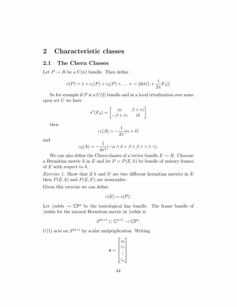
Let P → B be a U(n) bundle. Then define

c(P ) = 1 + c1(P ) + c2(P ) + . . . + = [det(1 +i

2πFA)]

So for example if P is a U(2) bundle and in a local trivalization over someopen set U we have

s∗(FA) =

[iα β + iγ

−β + iγ iδ

]then

c1(A) = − 1

2π(α + δ)

and

c2(A) = − 1

4π2(−α ∧ δ + β ∧ β + γ ∧ γ).

We can also define the Chern-classes of a vector bundle E → B. Chooosea Hermitian metric h in E and let P = P (E, h) be bundle of unitary framesof E with respect to h.

Exercise 1. Show that if h and h′ are two different hermitian metrics in Ethen P (E, h) and P (E, h′) are isomorphic.

Given this exercise we can define

c(E) = c(P ).

Let 〈mbda → CPn be the tautological line bundle. The frame bundle of〈mbda for the natural Hermitian metric in 〈mbda is

S2n+1 ⊂ Cn+1 → CPn.

U(1) acts on S2n+1 by scalar mulptiplication. Writing

z =

z0

z1...zn

44

the hermitian inner product is

h(z,w) = ztw

and the real inner product is the real part of this.

〈nglez,w〉 = <(ztw)

The infinitesimal generator of the action is

ξ = iz

The natural connection is the map

AzTzS2n+1 → iR

given by projection onto the generator of the action which is explicity by

Az(w) = i〈ngleiz,w〉 = −=(ztw).

Introduction the complex valued one forms

dzµ = dxµ + idyµ and dzµ = dxµ − idyµ

we can write this more tidily as

A = −=(ztdz)

Thus the curvature of A is

FA = dA = −=(dzt ∧ dz).

Here the curvature is written as a two-form on the total space of the bun-dle. To sort out which cohomology class c1(〈mbda) repersents it suffices toevaluate it on CP1 ⊂ CPn or more explicitly let φ : C → CPn be given by

φ(z) = [z : 1 : 0 : 0 : . . . 0].

φ lifts to cover a section of the bundle φ : C → S2n+1 given by

φ(z) = (z√

1 + |z|2,

1√1 + |z|2)

, 0, . . . , 0).

45

Then we must computei

2π

∫C

φ∗(FA)

φ∗(FA) = −=(dz√

1 + |z|2∧ d

z√1 + |z|2

+ d1√

1 + |z|2∧ d

1√1 + |z|2

= −=(dz ∧ dz

(1 + |z|2)2

= 2idx ∧ dy

(1 + x2 + y2)2

But from 18.01 we have∫R2

dx ∧ dy

(1 + x2 + y2)2= 2π

∫ ∞

0

rdr

(1 + r2)2

= π

And so all together we have

〈nglec1(〈mbda), [CP1]〉 =i

2π(2i)π = −1.

Whitney sum formula. If E = E1 ⊕ E2 then we have

Proposition 2.1. c(E) = c(E1)c(E2)

If E → B is complex vector bundle then we can form the conjugatebundle E. As real bundles E and E are isomorphic but z ∈ C acts on v ∈ Eby

z • v = zv.

2.2 The Pontryagin classes

Let V be a real vector bundle. The Pontryagin classes are defined to bethe Chern classes of the complexification with a sign twist that is the morecommon convention in the literature.

pi(V ) = (−1)ic2i(V ⊗R C) ∈ H2i(B; R)

46

However to keep life from getting too complicated we will define the totalPontryagin class to be

p(V ) = 1− p1(V ) + p2(V )− p3(V ) + . . . .

so that we can writep(V ) = c(V ⊗R C)

Properties. If V = V1 ⊕ V2 then

p(V ) =

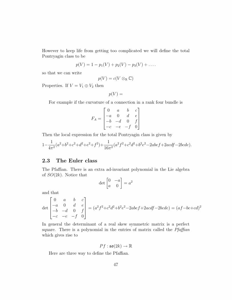
For example if the curvature of a connection in a rank four bundle is

FA =

0 a b c−a 0 d e−b −d 0 f−c −e −f 0

Then the local expression for the total Pontryagin class is given by

1− 1

4π2(a2+b2+c2+d2+e2+f 2)+

1

16π2(a2f 2+c2d2+b2e2−2abef+2acdf−2bcde).

2.3 The Euler class

The Pfaffian. There is an extra ad-invariant polynomial in the Lie algebraof SO(2k). Notice that

det

[0 −aa 0

]= a2

and that

det

0 a b c−a 0 d e−b −d 0 f−c −e −f 0

= (a2f 2+c2d2+b2e2−2abef+2acdf−2bcde) = (af−be+cd)2

In general the determinant of a real skew symmetric matrix is a perfectsquare. There is a polynomial in the entries of matrix called the Pfaffianwhich gives rise to

Pf : so(2k) → RHere are three way to define the Pfaffian.

47

1. Any 2k × 2k skew symmetric real matrix is conjugate by a matrix inSO(2k) to a matrix of the form

Λ =

0 −λ1 0 . . . 0λ1 0 0 . . . 00...0 0 −λk

0 λk 0

(A Cartan subalgebra of the Lie algebra so(2k).) Then we define

Pfaff(Λ) = λ1λ2 . . . λk

2.

3. Associate to M ∈ so(2k) the 2-form

M =∑i<j

Mijei ∧ ej.

Then Mk ∈ λ2k(R2k) and we define

1

k!Mk = Pfaff(M)e1 ∧ e2 . . . e2k

So for example Λ = λ1e1 ∧ e2 + . . . λke

2k−1 ∧ e2k.

3 Applications of Characteristic classes

You will have shown in your homework that

c(CP) = (1 + x)n+1

where x = −c1(〈mbda∗) ∈ H2(CPn.

48