Exponentially A urate Quasimodes for theTime{Independent Born{Oppenheimer Approximation ona One{Dimensional Mole ular SystemGeorge A. Hagedorn�Department of Mathemati s andCenter for Statisti al Me hani s and Mathemati al Physi sVirginia Polyte hni Institute and State UniversityBla ksburg, Virginia 24061{0123, U.S.A.andJulio H. TolozayCentro de Investiga i�on en Matem�ati asUniversidad Aut�onoma del Estado de HidalgoCarretera Pa hu a{Tulan ingo Km. 4.5Pa hu a de Soto, Hidalgo, CP 42090, M�exi oAbstra tWe onsider the eigenvalue problem for a one-dimensional mole ular{type quantumHamiltonian that has the formH(�) = � �42 �2�y2 + h(y);where h(y) is an analyti family of self-adjoint operators that has an dis rete, nonde-generate ele troni level E(y) for y in some open subset of R. Near a lo al minimum ofthe ele troni level E(y) that is not at a level rossing, we onstru t quasimodes that areexponentially a urate in the square of the Born{Oppenheimer parameter � by optimaltrun ation of the Rayleigh{S hr�odinger series. That is, we onstru t an energy E� and awave fun tion ��, su h that the L2-norm of �� is O(1) and the L2-norm of (H(�) � E�) ��is bounded by � exp ���=�2 � with � > 0.�Partially supported by National S ien e Foundation Grant DMS{0303586.yPartially supported by Se retar��a de Edu a i�on P�ubli a{PROMEP Grant UAEHGO{PTC{198.1

1 Introdu tionIn this paper we onstru t exponentially a urate quasimodes for the time{independent S hr�o-dinger equation for a simple mole ular system. The small parameter that governs the approx-imation is the usual Born{Oppenheimer parameter �, where �4 is the ele tron mass divided bythe mean nu lear mass. Under appropriate ir umstan es, the quasimodes we produ e orre-spond exa tly to the low{lying energy levels of the system. In that ase, the exa t eigenvaluesand our quasimode energies di�er by at most � exp (��=�2 ). A bound of the same formholds for the norm of the di�eren e between the quasimodes and the exa t eigenve tors.Hamiltonians for mole ular systems an generally be put in the formH(�) = � �42 �y + h(y);where the variable y des ribes the nu lear on�guration ve tor and the operator h(y) is theele tron Hamiltonian. In this paper we examine the spe ial ase of operators of this type, wherey is a single real variable, and h(y) is a family of (possibly unbounded) self{adjoint operators.There are three motivations for studying this somewhat unphysi al model. First, few rigor-ous exponentially a urate results for the time{independent Born{Oppenheimer approximationhave been published, and they do not over this model. Indeed, the only previous results ofthis kind, to the best of our knowledge, is our study of the spe ial ase where h(y) is a 2 � 2real symmetri matrix [9℄. Se ond, we onsider the treatment of this model as an intermediatestage toward the study of more realisti mole ular systems. We hope to be able to onstru texponentially a urate quasimodes for diatomi mole ules, using the te hniques developed in[9℄ and in this paper, although several te hni al diÆ ulties are yet to be over ome. Finally,we believe that the results we present are nevertheless interesting in themselves, be ause theygeneralize those of [9℄ to a mu h larger lass of situations with a relatively small amount ofwork. Most of the heavy omputations have been done in [9℄. Although the te hni al detailsare somewhat di�erent, we essentially redu e the present problem to the one studied in [9℄.To state our results pre isely, we need some notation and hypotheses. For small �, we studythe eigenvalue problem �� �42 d2dy2 + h(y) � (�; y) = E(�) (�; y);where h(y) denotes a family of operators that satis�es the following onditions:1. h(y) : He ! He is a self{adjoint operator for every y 2 R, where the ele troni Hilbertspa e He is separable. We furthermore assume that inf �(h(y)) is uniformly boundedfrom below.2. h(y) is an analyti family of type (A) in a neighborhood S � C of the origin. Fromhypothesis 1, it follows that h(y)? = h(y) for y 2 S.2

3. We assume h(0) has an isolated, non-degenerate eigenvalue E(0).By standard results, these hypotheses imply that h(y) has an isolated, non-degenerate eigen-value E(y) that depends analyti ally on y in a neighborhood S 0 � S of the origin. The asso iatedproje tion P (y) is analyti for y 2 S 0, and it is orthogonal for real y. The y-independent domainD of h(y) is a dense subspa e of the ele troni Hilbert spa e He. Finally we assume:4. E(y) has a non-degenerate lo al minimum at y = 0, i.e., E 0(0) = 0 and E 00(0) > 0.Without loss we assume that E(0) = 0 and E 00(0) = 1.An eigenfun tion (�; y) of H(�) belongs to L2(R;He), whose norm we denote by jjj�jjj.Under these hypotheses, we have the following result:Theorem 1 Assume hypotheses 1{4, and let � be a �xed non-negative integer. Then, usingoptimal trun ation of a perturbation expansion in powers of �, we an onstru t E� and ��, su hthat jjj�� jjj = O(1), E� = (� + 1=2) �2 + O(�4), andjjj (H(�)� E�) �� jjj < � exp ���=�2 � :This quasimode is asso iated with the �th vibrational energy level in the lo al well of E neary = 0.Remarks. 1. Our hypotheses allow level rossings as well as merging of E into the ontin-uous spe trum, as long as these phenomena do not o ur at the bottom of the lo al well of Ewhere �� is on entrated.2. Our quasienergy E� may lie within the essential spe trum. In that ase, one would expe ta resonan e near our quasienergy asso iated with the system being temporarily trapped in thewell.3. If inf (�(h(y)) n E(y)) > 0, lim infjyj!1 E(y) > 0, and E has a unique global minimum atzero, then for small �, the quasimode of the theorem is an exponentially a urate approximationto the �th eigenvalue of H(�). This is proved by ombining our results with those of [3℄.4. The assumption that inf �(h(y)) is bounded below is just used to guarantee self{adjointnessof H(�). It never enters dire tly into our al ulations, and it ould be weakened.5. Our estimates depend in ompli ated ways on various parameters of the problem. We havenot kept tra k of the dependen e of � and � on these parameters. We anti ipate that doing sowould be very tedious.The time{independent Born{Oppenheimer approximation has a long history that dates ba kto [2℄. The �rst mathemati ally rigorous result about its validity for low{lying states is [3℄, inwhi h the expansion for the energy is proved to be a urate through fourth order in �. Rigorousexpansions to all orders are developed for systems with smooth potentials [4℄, diatomi Coulomb3

systems [5℄, and general Coulomb systems [13℄. As we have already mentioned, the only previous onstru tion of approximate solutions up to exponentially small errors is developed by theauthors in [9℄.Various other authors have studied time{independent Born{Oppenheimer limits for other prob-lems. Sordoni [20℄ has extended the results mentioned above to in lude high angular momentumstates of diatomi mole ules. Herrin and Howland [10℄ have studied a situation in whi h thebundle of eigenve tors for the ele tron Hamiltonian had a non{trivial Berry phase. Rousse [19℄has onstru ted quasimodes at �xed energies above the bottoms of wells when the nu lei haveone degree of freedom. His results involved Bohr{Sommerfeld rules, and he handled level ross-ings and avoided rossings whose gaps had ertain � dependen e. Klein, Martinez, and Messirdi[12, 14, 15, 17℄ have studied resonan es whose lifetimes are �nite be ause non{adiabati tran-sitions of the ele trons oupled them to the ontinuous spe trum. In losely related subje ts,we note rigorous exponentially a urate results for the time{dependent Born{Oppenheimerapproximation [8, 16, 18℄ and for lifetimes of resonan es [15, 17℄.The paper is organized as follows: In Se tion 2, we derive the formal perturbation expansionthat we use to prove Theorem 1. In Se tion 3, we study the growth of quantities that o urin the perturbation expansion. Then in Se tion 4, we prove the error bounds that implyTheorem 1.2 The Perturbation ExpansionOur onstru tion of the quasimodes involves the omputation of formal Rayleigh{S hr�odingerseries in powers of �, whose oeÆ ients belong to the following Hilbert spa es:1. The nu lear Hilbert spa e L2(R) (with Lebesgue measure), whose inner produ t and normwe denote respe tively by ( �; � ) and k � k.2. The ele troni Hilbert spa e He. The inner produ t and the norm we denote by h �; � iand k � ke.3. The mole ular Hilbert spa e L2(R;He). The inner produ t is de�ned byZR h�(x); (x)i dx:As already mentioned, we denote its norm by jjj�jjj.The operator h(y) an be de omposed ash(y) = E(y)P (y) + h?(y);where h?(y) := h(y)(1� P (y)) is an analyti family of type (A) in some neighborhood S 00 �S 0 � S around the origin. By shrinking S 00 if ne essary, we may assume that 0 belongs to the4

resolvent set of the restri tion of h?(y) to the range of (1� P (y)) for y 2 S 00. We let h?(0)�1denote the redu ed resolvent that is 0 in the range on P (0). Hen eforth, we assume that allthe analyti properties used in the treatment of this problem are valid in the region S 00.After making the onvenient s aling y = � x, the eigenvalue equation be omes�� �22 d2dx2 + h(�x) � (�; x) = E(�) (�; x); (1)where (�; x) 2 L2(R;He). With a slight abuse of notation, we hen eforth denote the Hamil-tonian operator in (1) by H(�).The fun tion an be de omposed as(�; x) = w(�; x) �(�x) + ?(�; x);where �(y) is the eigenve tor asso iated to E(y) and h�(�x); ?(�; x)i = 0 for ea h x. We hoose �(y) to be analyti for y 2 S 00 and normalized when y 2 S 00 is real. We hoose itsphase so that h�(y); �0(y)i = 0. Sin e ?(�; x) = (1� P (�x)) ?(�; x), the �rst and se ondderivatives of (�; x) are given by�x = (�xw) � + � w�0 � � P 0? + (1� P ) �x?; and�2x = (�2xw) � + 2 � (�xw) �0 + �2w�00 � �2 P 00? � 2 � P 0 �x? + (1� P ) �2x?= ��2xw + 2 � h�;�0i �xw � 2 � h�; P 0�x?i+ �2w h�;�00i � �2 h�; P 00?i��+ (1� P ) ��2x? + 2 � (�xw) �0 � 2 � P 0 �x? + �2w�00 � �2 P 00?� :Thus, in a neighborhood of 0, equation (1) is equivalent to the following pair of equations:��22 �2xw � �3 h�;�0i �xw + �3 h�; P 0�x?i � �42 w h�;�00i+ �42 h�; P 00?i+ Ew = Ew; (2)and ��22 (1� P )�2x? � �3(�xw)(1� P )�0 + �3(1� P )P 0�x?� �42 w(1� P )�00 + �42 (1� P )P 00? + h?(1� P )? = E(1� P )?: (3)In order to take full advantage of the work done in [9℄, it is onvenient to ast these equationsin forms that resemble equations (3) and (4) of that paper. We �rst note thatP = h�; � i�;P 0 = h�; � i�0 + h�0; � i�;P 00 = h�; � i�00 + 2 h�0; � i�0 + h�00; � i�;PP 0 = h�0; � i�; andPP 00 = h�; �00i h�; � i� + h�00; � i�:5

The last two identities follow from our phase ondition h�; �0i = 0 on �. It thus follows thath�0; �0i = �h�; �00i = �h�00; �i. Also, from h�; ?i = 0, we easily obtainh�; �x?i = � � h�0; ?i ; and�; �2x?� = � 2 � h�0; �x?i + �2 h�00; ?i :With the use of these identities, equations (2) and (3) be ome� �22 �2xw + �3 h�0; �x?i � �42 w h�00; �i + �42 h�00; ?i + E w = E w; (4)and � �22 �2x? � �3 ( �xw�0 + h�0; �x?i � )� �42 w (�00 � h�; �00i�) � �42 h�00; ?i � + h?? = E ?: (5)In order to simplify some expressions, we introdu e the following notation:A(z) = �0(z);B(z) = h�00(z); �(z)i ;C(z) = �00(z);F(z) = �00(z) � h�(z); �00(z)i �(z);G(z) = h�0(z); � i �(z); andK(z) = h�00(z); � i �(z):Note that A, C and F are ve tor{valued fun tions, whereas G and K are operator{valuedfun tions. All these fun tions are analyti in S 00. Equations (4) and (5) an now be written as� �22 �2xw + �3 hA; �x?i � �42 Bw + �42 hC; ?i + E w = E w; (6)and � �22 �2x? � �3 ( �xwA + G �x? ) � �42 wF � �42 K? + h?? = E ?: (7)The fun tions de�ned above, along with E(z) and �(z), have onvergent Taylor series in aneighborhood of 0. We denote these asE(�x) = 12 �2 x2 + 1Xn=3 dn �n xn;6

�(�x) = 1Xn=0 �n �n xn;A(�x) = 1Xn=0 an �n xn;B(�x) = 1Xn=0 bn �n xn;C(�x) = 1Xn=0 n �n xn;F(�x) = 1Xn=0 fn �n xn;G(�x) = 1Xn=0 gn �n xn; andK(�x) = 1Xn=0 kn �n xn:The oeÆ ients �n, an, n, and fn are ve tors in He. The oeÆ ients gn and kn are boundedlinear operators on He that satisfy the identitiesgn = nXp=0 hap; � i �n�p; andkn = nXp=0 h p; � i �n�p:A similar expansion an be performed on the (unbounded) operator{valued fun tion h?(�x).Sin e h? is an analyti family in the sense of Kato, there exists a olle tion of operatorsh?;n : D !He, all relatively bounded with respe t to h?;0 := h?(0), su h thath?(�x)� = 1Xn=0 �n xn h?;n�in the strong sense, for every �x lose to 0 and every � 2 D.We now repla e E(�), w(�; x) and ?(�; x) by their formal Rayleigh{S hr�odinger series,E(�) = 1Xn=0 En �n;w(�; x) = 1Xn=0 wn(x) �n;?(�; x) = 1Xn=0 ?;n(x) �n:7

We insert all these series into the equations (6) and (7) and equate terms of the same orders in� on the two sides of the equations. This yields the following:Order 0 : E0 w0 = 0; andh?;0 ?;0 = E0 ?;0:Sin e we want w0 6= 0, the �rst equation requires E0 = 0. Sin e 0 62 � (h?;0), the se ondequation for es ?;0 = 0.Order 1 : E0 w1 + E1 w0 = 0; andh?;0 ?;1 + x h?;1 ?;0 = E0 ?;1 + E1 ?;0:The �rst equation requires E1 = 0. The se ond equation then for es ?;1 = 0.Order 2 : � 12 �2x w0 + 12 x2 w0 = E2 w0; andh?;0 ?;2 = 0:Clearly E2 and w0 must be solutions to the eigenvalue problem for the harmoni os illatorHamiltonian H0 = � 12 d2dx2 + 12 x2;whose eigenvalues and normalized eigenfun tions are (�+1=2) and ��(x), where � = 0; 1; 2; 3; : : :We �x a hoi e of � and then have E2 = (�+1=2), and w0 = ��. The se ond equation requires?;2 = 0.Order 3 : (H0 � E2) w1 + ha0; �x?;0i + d3 x3 w0 = E3 w0; and� (�xw0) a0 + h?;0 ?;3 = 0:Equating omponents in the dire tion of �� in the �rst equation leads to E3 = 0. Theorthogonal omponents then requirew1 = � d3 (H0 � E2)�1? x3 w0;where (H0�E2)�1? denotes the inverse of the restri tion of (H0�E2) to the subspa e orthogonalto ��. We hen eforth arbitrarily assume that wn ? �� for all n > 0. The se ond equationyields ?;3 = (�xw0) (h?;0)�1 a0:8

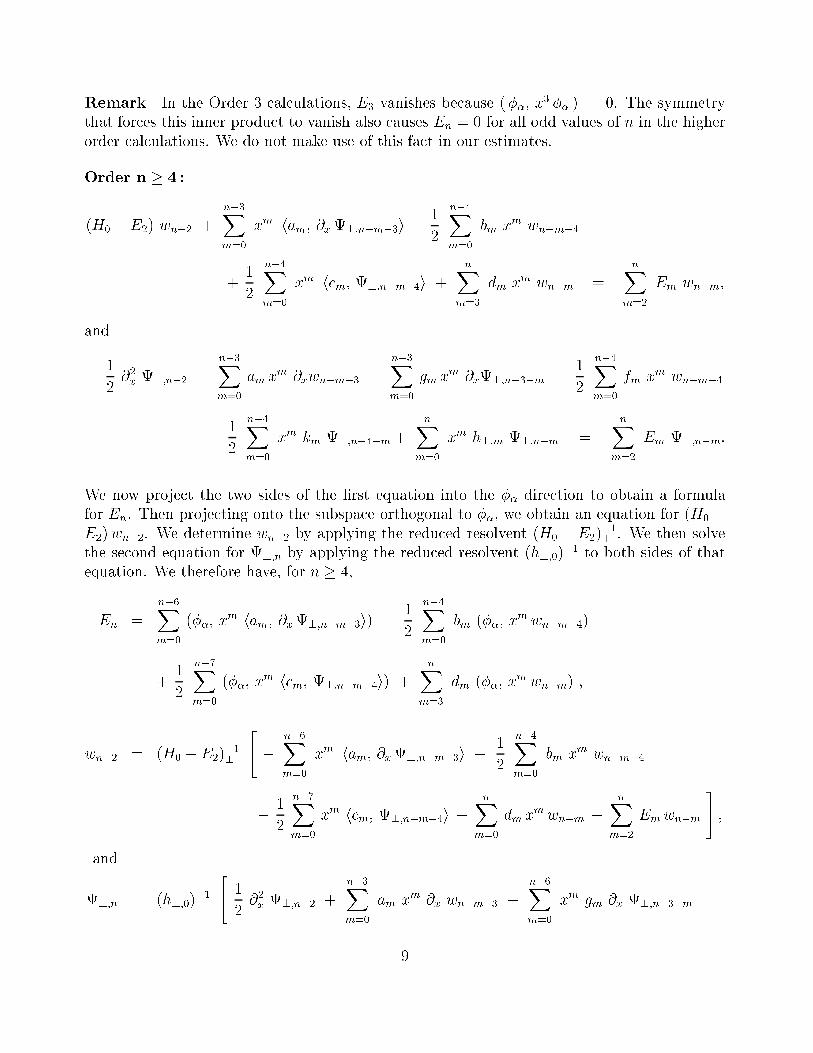
Remark In the Order 3 al ulations, E3 vanishes be ause (��; x3 �� ) = 0. The symmetrythat for es this inner produ t to vanish also auses En = 0 for all odd values of n in the higherorder al ulations. We do not make use of this fa t in our estimates.Order n � 4 :(H0 � E2) wn�2 + n�3Xm=0 xm ham; �x?;n�m�3i � 12 n�4Xm=0 bm xm wn�m�4+ 12 n�4Xm=0 xm h m; ?;n�m�4i + nXm=3 dm xm wn�m = nXm=2 Em wn�m;and� 12 �2x ?;n�2 � n�3Xm=0 am xm �xwn�m�3 � n�3Xm=0 gm xm �x?;n�3�m � 12 n�4Xm=0 fm xm wn�m�4� 12 n�4Xm=0 xm km ?;n�4�m + nXm=0 xm h?;m ?;n�m = nXm=2 Em ?;n�m:We now proje t the two sides of the �rst equation into the �� dire tion to obtain a formulafor En. Then proje ting onto the subspa e orthogonal to ��, we obtain an equation for (H0 �E2)wn�2. We determine wn�2 by applying the redu ed resolvent (H0 � E2)�1? . We then solvethe se ond equation for ?;n by applying the redu ed resolvent (h?;0)�1 to both sides of thatequation. We therefore have, for n � 4,En = n�6Xm=0 (��; xm ham; �x?;n�m�3i) � 12 n�4Xm=0 bm (��; xm wn�m�4)+ 12 n�7Xm=0 (��; xm h m; ?;n�m�4i) + nXm=3 dm (��; xm wn�m) ;wn�2 = (H0 � E2)�1? " � n�6Xm=0 xm ham; �x?;n�m�3i + 12 n�4Xm=0 bm xm wn�m�4� 12 n�7Xm=0 xm h m; ?;n�m�4i � nXm=0 dm xm wn�m + nXm=2 Em wn�m # ;and?;n = (h?;0)�1 " 12 �2x ?;n�2 + n�3Xm=0 am xm �x wn�m�3 + n�6Xm=0 xm gm �x ?;n�3�m9

� 12 n�4Xm=0 fm xm wn�m�4 � 12 n�7Xm=0 xm km ?;n�4�m+ n�3Xm=1 xm h?;m?;n�m + n�3Xm=2 Em ?;n�m # :In the sequel, we use the fa t that L2(R;He) is isomorphi to L2(R) He. LetU : L2(R) He ! L2(R;He) denote the natural isomorphism de�ned byU(�(x)�) = �(x)�:Although the set of re ursive equations given above involves ertain unbounded operators, they an be redu ed to bounded operators be ause of the following result.Lemma 1 Let Pi�n denote the proje tion onto the span of �i's with 0 � i � n. Thenwn 2 Ran (Pi�3n+�) for all n � 0;?;n 2 Ran (U (Pi�3n+��8 I)U?) for all n � 3:Proof: We prove this by an easy indu tion using the equations that de�ne wn�2 and n. 2In order to obtain estimates that are sharp enough for our purposes, we transform the problem,using a method originally developed in [21, 22℄. We introdu e a bounded operator A, whi hdepends on the hoi e of �, by de�ning its a tion on the basis of the harmoni os illatorHamiltonian: A�� = ( �� if � = �;j� � �j�1=2 �� if � 6= �:We then de�ne ~A : L2(R;He) ! L2(R;He) as ~A = U(A I)U?. These operators satisfy thefollowing identity.Lemma 2 Consider any (x) 2 L2(R;He) and � 2 He. Then,h�; U(A I)U?(x)i = A h�; (x)i :As a onsequen e, the operators gm and km all ommute with ~A.Proof: Let f�mg be a basis of He and f��(x)g a basis of L2(R). Then f��(x)�mg is a basisof L2(R;He) andh�; U(A I)U?(��(x)�m)i = h�; U(A I)(��(x)�m)i10

= h�; U((A��)(x) �m)i= h�; (A��)(x)�mi= (A��)(x) h�; �mi= A h�; ��(x)�mi :Now extend by linearity. 2Rather than estimating the norms of wn and ?;n dire tly, we study wn and ?;n, wherewn = A wn and ?;n = h�1?;0 ~A ?;n = ~Ah�1?;0 ?;n. These de�nitions make sense be ause all�nite linear ombinations of �i's are in the domain of the unbounded operator A�1. We de�ne~A�1 = U(A�1 I)U?. In addition, we multiply (6) and (7) by A and ~A respe tively. Afterwardwe use Lemma 2. In this manner we obtain the following:E0 = E1 = E3 = 0;E2 = � + 1=2;w0 = ��;w1 = � d3 [A(H0 � E2)A℄�1? Ax3A w0;?;0 = ?;1 = ?;2 = 0;?;3 = ~A�1 (�xw0) a0;and for n � 4,En = n�6Xm=0 �A�x xm A��; Dam; h�1?;0 ?;n�m�3E� � 12 n�4Xm=0 bm (Axm A��; wn�m�4)+ 12 n�7Xm=0 �AxmA��; D m; h�1?;0 ?;n�m�4E� + nXm=3 dm (AxmA��; wn�m) ;wn�2 = [A(H0 � E2)A℄�1? "� n�6Xm=0Axm �xADam; h�1?;0 ?;n�m�3E+ 12 n�4Xm=0 bm AxmA wn�m�4� 12 n�7Xm=0 AxmAD m; h�1?;0 ?;n�m�4E � nXm=3 dmAxmA wn�m+ nXm=2Em A2 wn�m # ;and 11

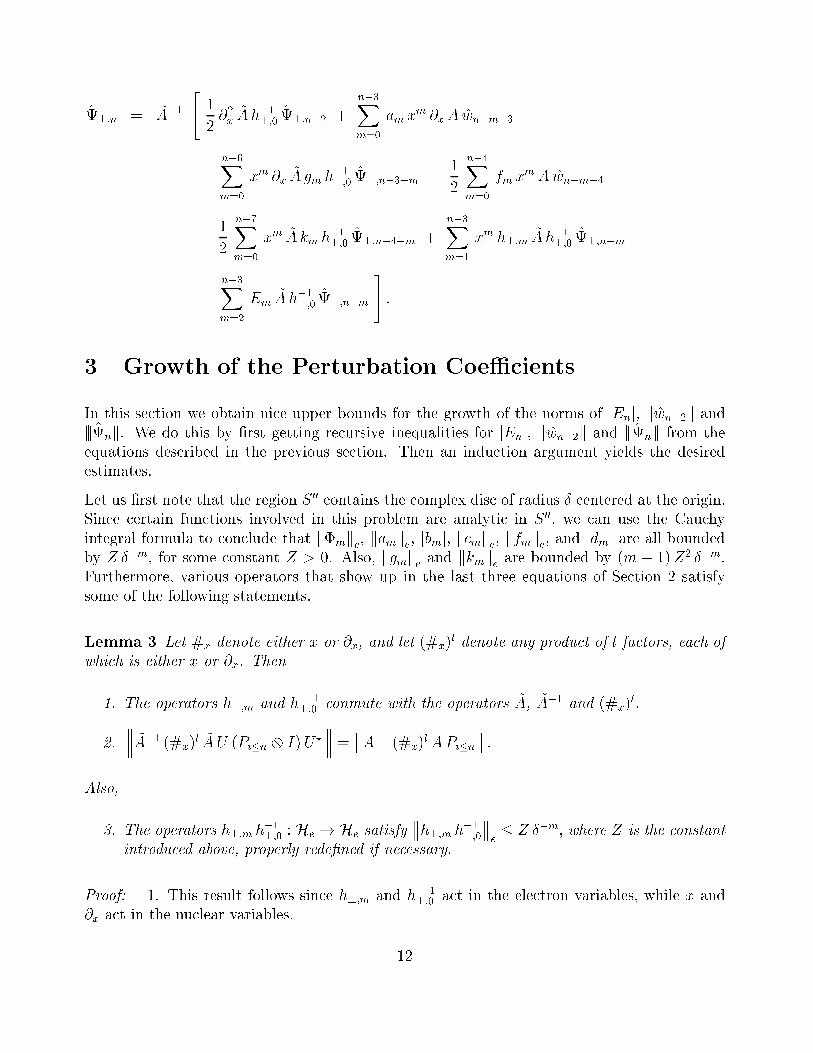
?;n = ~A�1 " 12 �2x ~Ah�1?;0 ?;n�2 + n�3Xm=0 am xm �xA wn�m�3+ n�6Xm=0 xm �x ~Agm h�1?;0 ?;n�3�m � 12 n�4Xm=0 fm xm A wn�m�4� 12 n�7Xm=0 xm ~Akm h�1?;0 ?;n�4�m + n�3Xm=1 xm h?;m ~Ah�1?;0 ?;n�m+ n�3Xm=2 Em ~Ah�1?;0 ?;n�m # :3 Growth of the Perturbation CoeÆ ientsIn this se tion we obtain ni e upper bounds for the growth of the norms of jEnj, kwn�2k andjjjnjjj. We do this by �rst getting re ursive inequalities for jEnj, kwn�2k and jjjnjjj from theequations des ribed in the previous se tion. Then an indu tion argument yields the desiredestimates.Let us �rst note that the region S 00 ontains the omplex dis of radius Æ entered at the origin.Sin e ertain fun tions involved in this problem are analyti in S 00, we an use the Cau hyintegral formula to on lude that k�mke, kamke, jbmj, k mke, kfmke, and jdmj are all boundedby Z Æ�m, for some onstant Z > 0. Also, kgmke and kkmke are bounded by (m + 1)Z2 Æ�m.Furthermore, various operators that show up in the last three equations of Se tion 2 satisfysome of the following statements.Lemma 3 Let #x denote either x or �x, and let (#x)l denote any produ t of l fa tors, ea h ofwhi h is either x or �x. Then1. The operators h?;m and h �1?;0 onmute with the operators ~A, ~A�1 and (#x)l.2. ��������� ~A�1 (#x)l ~AU (Pi�n I)U?��������� = A�1 (#x)l APi�n :Also,3. The operators h?;m h�1?;0 : He ! He satisfy h?;m h�1?;0 e � Z Æ�m; where Z is the onstantintrodu ed above, properly rede�ned if ne essary.Proof: 1. This result follows sin e h?;m and h �1?;0 a t in the ele tron variables, while x and�x a t in the nu lear variables. 12

2. This result is a onsequen e of the ele troni variables playing no signi� ant role in theoperators involved.3. We have assumed that h(�) is an analyti family of type (A) with domain D. By resultsof Se tion 2 of Chapter 7 of [11℄, it follows that h(y) h �1?;0 is a bounded analyti family on He.The Taylor series oeÆ ients of this operator valued fun tion are h?;m h�1?;0, and the radius of onvergen e is at least Æ. The result follows from the standard Cau hy estimates. 2Using Lemmas 1 and 3 we obtain the following set of inequalities:jEnj � Z n�6Xm=0 Æ�mkA�x xmAPi��k ���������?;n�m�3��������� + Z2 n�4Xm=0 Æ�mkAxmAPi��kkwn�m�4k+ Z2 n�7Xm=0 Æ�mkAxmAPi��k ���������?;n�m�4��������� + Z nXm=3 Æ�mkAxmAPi��kkwn�mk ;kwn�2k � Z n�6Xm=0 Æ�mkA�x xmAPi�3(n�m�3)+��8k ���������?;n�m�3���������+ Z2 n�4Xm=0 Æ�mkAxmAPi�3(n�m�4)+�kkwn�m�4k+ Z2 n�7Xm=0 Æ�mkAxmAPi�3(n�m�4)+��8k ���������?;n�m�4���������+ Z nXm=3 Æ�mkAxmAPi�3(n�m)+�kkwn�mk + nXm=2 jEmjkwn�mk ;and���������?;n��������� � h�1?;0 e2 A�1 �2x ~APi�3(n�2)+��8 ���������?;n�2���������+ Z n�3Xm=0 Æ�m A�1 xm �xAPi�3(n�m�3)+� kwn�m�3k+ Z2 h�1?;0 e n�6Xm=0 Æ�m (m + 1) A�1 xm �xAPi�3(n�m�3)+��8 ���������?;n�m�3���������+ Z2 n�4Xm=0 Æ�m A�1 xm APi�3(n�m�4)+� kwn�m�4k13

+ Z2 h�1?;0 e2 n�7Xm=0 Æ�m (m + 1) A�1 xm APi�3(n�m�4)+��8 ���������?;n�m�4���������+ Z nXm=1 Æ�m A�1 xmAPi�3(n�m)+��8 ���������?;n�m���������+ h�1?;0 e nXm=0 jEmj ���������?;n�m��������� :These inequalities di�er only in unimportant ways from those pre eding (16) in [9℄. This leadsus to the following result.Theorem 2 De�ne � := 2=Æ2. There exists b > 1 su h that for every n � 3 we havejEnj < �3(n�2) b2n�5 [(n + �� 2)!℄1=2;kwn�2k < �3(n�2) b2n�3 [(n + �� 1)!℄1=2; and���������?;n��������� < �3n b2n�1 [(n + �� 1)!℄1=2:The rather tedious proof of this theorem is based on a simple indu tion argument. We refer tothe proof of Theorem 2 of [9℄ for the details.4 Estimates for the Norm of the ErrorThe onstru tion of the exponentially a urate quasimodes is based on trun ation of the formalRayleigh{S hr�odinger series whose oeÆ ients obey the growth estimates stated in Theorem 2.Here we mimi to a ertain extent the arguments in [21, 22℄, whi h are based on a te hniquedeveloped in [7℄. The main hange in our present ase is that the re ursion relations thatgenerate these oeÆ ients make sense only in a neighborhood of the bottom of the energysurfa e E(y). This issue will be dealt with by using a suitable ut{o� fun tion. In order toprove ertain estimates, we hen eforth assume that the region S 00 � C ontains the open setfz 2 C : jz + sj < Æ + �g [ fz 2 C : jz � sj < Æ + �g [ fz 2 C : jRe zj < s ; jIm zj < Æ + �g;for some �xed s > 0, 1 � Æ > 0 and � > 0 arbitrarily small.For N � 1 de�ne EN := N+2Xn=0 �nEn;14

wN(�; x) := NXn=0 �n wn(�; x);N?(�; x) := N+2Xn=0 �n?;n(�; x); andN(�; x) := wN(�; x) �(�x) + N? (�; x):Let f be a real C2 fun tion, su h that f(y) = 1 for y 2 [�r=�; r=�℄ and f(y) = 0 for y 62[�s=�; s=�℄, where s > r > 0. The support of f 0 is then ontained in [�s=�;�r=�℄ [ [r=�; s=�℄.For later use, let �f 0 denote the hara teristi fun tion of the support of f 0.We now de�ne �N (�; x) := f(x)N(�; x):Let H(�) denote the self{adjoint operator de�ned in equation (1). The error ommited whentrun ated Rayleigh{S hr�odinger series repla e the a tual solution to equation (1) is given by�H(�)� EN��N = f �H(�)� EN�N � �22 ��2x; f�N : (8)The �rst term an be written as (temporarily ignoring the ut{o�)�H(�)� EN�N = SN � + TN ;where the residual terms SN and TN are given expli itly bySN := � �22 �2x wN + �3 A; �xN?�� �42 BwN + �42 C; N?�+ E wN � EN wN ; andTN := � �22 �2xN? � �3 ��xwN A + G �xN?� � �42 wN F � �42 KN?+ h?N? � EN N? :Sin e the perturbation oeÆ ients are the solutions to the re ursive equations obtained inSe tion 2, all terms of order n � N + 2 an el in both SN and TN . Thus, the residual terms an be written asSN = NXm=0 �m+3 A[N�m�1℄; �x?;m� + �N+4 A[�1℄; �x?;N+1� + �N+5 A[�1℄; �x?;N+2�� 12 N�1Xm=0 �m+4 B[N�m�2℄wm � �N+42 B[�1℄wN+ 12 N�1Xm=0 �m+4 C [N�m�2℄; ?;m� 15

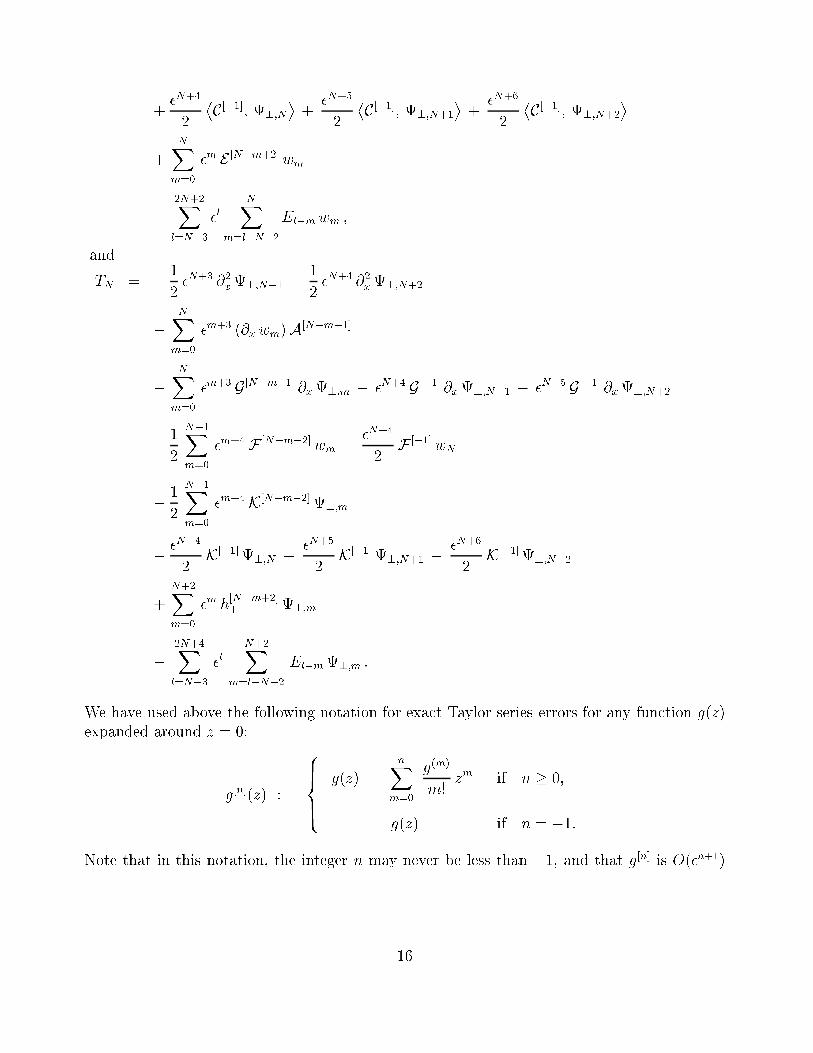
+ �N+42 C[�1℄; ?;N� + �N+52 C [�1℄; ?;N+1� + �N+62 C [�1℄; ?;N+2�+ NXm=0 �m E [N�m+2℄wm� 2N+2Xl=N+3 �l NXm=l�N�2El�m wm ;andTN = � 12 �N+3 �2x?;N+1 � 12 �N+4 �2x?;N+2� NXm=0 �m+3 (�xwm)A[N�m�1℄� NXm=0 �m+3 G[N�m�1℄ �x?;m � �N+4 G[�1℄ �x?;N+1 � �N+5 G[�1℄ �x?;N+2� 12 N�1Xm=0 �m+4 F [N�m�2℄wm � �N+42 F [�1℄wN� 12 N�1Xm=0 �m+4K[N�m�2℄?;m� �N+42 K[�1℄?;N � �N+52 K[�1℄?;N+1 � �N+62 K[�1℄?;N+2+ N+2Xm=0 �m h[N�m+2℄? ?;m� 2N+4Xl=N+3 �l N+2Xm=l�N�2 El�m?;m :We have used above the following notation for exa t Taylor series errors for any fun tion g(z)expanded around z = 0:g[n℄(z) := 8>><>>: g(z) � nXm=0 g(m)m! zm if n � 0;g(z) if n = �1:Note that in this notation, the integer n may never be less than �1, and that g[n℄ is O(�n+1)16

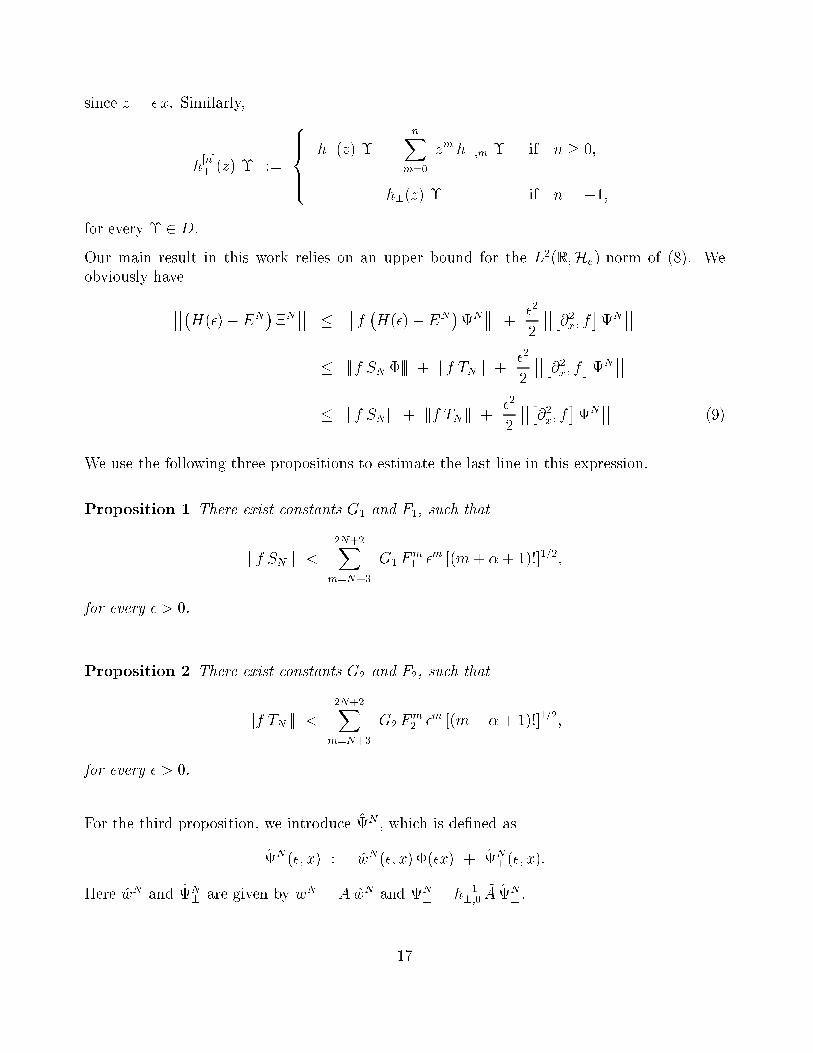
sin e z = � x. Similarly,h[n℄? (z) � := 8>><>>: h?(z) � � nXm=0 zm h?;m � if n � 0;h?(z) � if n = �1;for every � 2 D.Our main result in this work relies on an upper bound for the L2(R;He)-norm of (8). Weobviously have�������H(�)� EN��N ������ � ������f �H(�)� EN�N ������ + �22 ��������2x; f�N ������� jjjf SN �jjj + jjjf TN jjj + �22 ��������2x; f�N ������� kf SNk + jjjf TN jjj + �22 ��������2x; f�N ������ (9)We use the following three propositions to estimate the last line in this expression.Proposition 1 There exist onstants G1 and F1, su h thatkf SNk < 2N+2Xm=N+3 G1 Fm1 �m [(m+ � + 1)!℄1=2;for every � > 0.Proposition 2 There exist onstants G2 and F2, su h thatjjjf TN jjj < 2N+2Xm=N+3 G2 Fm2 �m [(m + � + 1)!℄1=2;for every � > 0.For the third proposition, we introdu e N , whi h is de�ned asN(�; x) := wN(�; x) �(�x) + N?(�; x):Here wN and N? are given by wN = A wN and N? = h�1?;0 ~A N? .17

Proposition 3 Let r and s be the numbers that de�ne the support of f 0. Then, for every � > 0that satis�es r2=�2 � 6N + 2�+ 3, we have��������2x; f�N ������ < G0(�) 23N+� exp �� r22�2��� r��12 ���������N ��������� ;whereG0(�) := kf 00k1 �1 + h�1?;0 2e�1=2 + 8 kf 0k1 k�xAk h�1?;0 e+ 8 kf 0k1 k�xAk2 + �2 supy2[�s;s℄ k�0(y)k2!1=2 :The proof of Proposition 1 is based on norm estimates for operators that are rank one in Hefor ea h x. In parti ular, let R : R ! He be ontinuous (or just lo ally L2(R;He)). Then learly f(x)R(x) 2 L2(R;He), where f is a ut{o� fun tion. Furthermore, f(x) hR(x); � i :L2(R;He)! L2(R) is a bounded linear operator. Sin ekf(x) hR(x); (x)ik2 = ZR f 2(x) jhR(x); (x)ij2 dx� ZR f 2(x) kR(x)k2e k(x)k2e dx� supy2supp (f) kR(y)k2e ZR k(x)k2e dx:;we have, kf(x) hR(x); � ik � supy2supp (f) kR(y)ke :Further onsequen es of this result are summarized in the following lemma:Lemma 4 Let R be an analyti He{valued fun tion, de�ned on the region S 00 (whi h dependson s > 0, 1 � Æ > 0 and � > 0). Let f be a ut{o� fun tion with support on [�s=�; s=�℄. Thenthere exists a onstant MR > 0, independent of � > 0, su h that:(i) k f(x) hR(�x); � i k � MR.(ii) For ea h � 2 (�jxj; jxj) and any pair of integers j and l that satisfy j � i and j + l � 0, f(x) xj+lj! R(j)(��); U(Pi�n I)U? � � � MR Æ�j 2 j+l2 �(n+ j + l)!n! �1=2 :18

Proof: Statement (i) is obvious. To prove (ii), �rst note that f(x) xj+lj! R(j)(��); U(Pi�n I)U? � � � f(x) 1j! R(j)(��); � � xj+lPi�n :Now use (i), the Cau hy Integral Formula to estimate R(j)(��) e =j!, and Lemma 5.1 of [7℄ toestimate xj+lPi�n . 2A similar result holds for analyti omplex{valued fun tions, whi h we state without proof.Lemma 5 Let D be an analyti omplex{valued fun tion, de�ned on the region S 00. Under thesame onditions as stated in Lemma 4, there exists a onstant MD > 0, independent of � > 0,su h that:(i) k f(x)D(�x) k � MD.(ii) For ea h � 2 (�jxj; jxj) and any pair of integers j and l that satisfy j � i and j + l � 0, f(x) xj+lj! D(j)(��) Pi�n � MD Æ�j 2 j+l2 �(n+ j + l)!n! �1=2 :Sket h of the proof of Proposition 1: We havekf SNk � NXm=0 �m+3 f A[N�m�1℄; �x?;m� + �N+4 f A[�1℄; �x?;N+1� + �N+5 f A[�1℄; �x?;N+2� + 12 N�1Xm=0 �m+4 f B[N�m�2℄ wm + �N+42 f B[�1℄ wN + 12 N�1Xm=0 �m+4 f C [N�m�2℄; ?;m� + �N+42 f C [�1℄; ?;N� + �N+52 f C [�1℄; ?;N+1� + �N+62 f C [�1℄; ?;N+2� + NXm=0 �m f E [N�m+2℄wm + 2N+2Xl=N+3 �l NXm=l�N�2 jEl�mj kwmk : (10)We now apply Lemma 4, Lemma 5, and Theorem 2. This leads to an upper bound for kf SNkthat looks nearly identi al to the right-hand side of inequality (30) of [9℄. The statement of theproposition then follows from the proof of Theorem 3 of that paper. 219

Sket h of the proof of Proposition 2: The strategy is the same as for Proposition 1. How-ever, there is a ompli ation be ause our expression for TN ontains more terms than in the orresponding expression in [9℄.By the triangle inequality and our expression for TN , we havejjjf TN jjj = 12 �N+3 ������ f �2x?;N+1 ������ + 12 �N+4 ������ f �2x?;N+2 ������+ NXm=0 �m+3 ������ f (�xwm)A[N�m�1℄ ������ + NXm=0 �m+3 ������ f G [N�m�1℄ �x?;m ������+ �N+4 ������ f G[�1℄ �x?;N+1 ������ + �N+5 ������ f G[�1℄ �x?;N+2 ������+ 12 N�1Xm=0 �m+4 ������ f F [N�m�2℄ wm ������ + �N+42 ������ f F [�1℄ wN ������+ 12 N�1Xm=0 �m+4 ������ f K[N�m�2℄ ?;m ������ + �N+42 ������ f K[�1℄ ?;N ������+ �N+52 ������ f K[�1℄ ?;N+1 ������ + �N+62 ������ f K[�1℄ ?;N+2 ������+ N+2Xm=0 �m ��������� f h[N�m+2℄? ?;m ��������� + 2N+4Xl=N+3 �l N+2Xm=l�N�2 jEl�mj jjj?;mjjj : (11)We refer to the terms in this expression (in order) as terms 1, 2, . . . , 14. Terms 1{3, 7{14are ompletely analogous to terms 1{11 of equation (35) of [9℄ (in the same order), and theyrespe tively satisfy the orresponding bounds as in [9℄. As with Proposition 1 the proof of thisrequires the use of Lemmas 4, 5 (with slight modi� ations), and Theorem 2. Terms 4{6 in (11)do not o ur in equation (35) of [9℄, but they arise in the same way as the �rst three terms in(10) (or equivalently as the �rst four terms in equation (35) of [9℄). Sin e the operator normsof G[j℄ and ve tor norms of A[j℄ satisfy the same types of bounds, the norms of terms 4{6 of(11) satisfy the same bounds as the norms of the �rst three terms of (10).The Proposition follows sin e the norm of every term in (11) is bounded by some onstanttimes Fm2 �m [(m + � + 1)!℄1=2, for some F2, where N + 2 � m � 2N + 2. 2Proposition 3 is essentially a onsequen e of �f 0 pi king up only the exponentially de ayingportion of the lower{order eigenfun tions of the harmoni os illator Hamiltonian H0. Morepre isely, we have the following lemma.Lemma 6 For any non-negative integer n and every � > 0 that satisfy r2=�2 � 2n+1, we havek�f 0 Pi�n k < 2n exp �� r22�2��� r��12 :20

Proof: Consider any ' = Pni=0 di �i, where the �i's are the normalized eigenfun tions of H0.Then, k�f 0 Pi�n ' k � nXi=0 jdij k�f 0�i k � nXi=0 jdij2! 12 nXi=0 k�f 0 �i k2! 12 :Therefore, k�f 0 Pi�n k � nXi=0 k�f 0 �i k2! 12 :Re all that �i(x) = p�1=2 2i i! exp(�x2=2) Hi(x), where the Hermite polynomialsHi(x) satisfythe inequality jHi(x)j � 2ijxji for x � p2i+ 1, as proved in Lemma 3.1 of [6℄. Thus,nXi=0 k�f 0 �i k2 = nXi=0 ZR �f 0(x) j�i(x)j2 dx� 2 nXi=0 Z 1r=� j�i(x)j2 dx� 2�1=2 nXi=0 2ii! Z 1r=� e�x2 x2i dx< 2�1=2 4n Z 1r=� e�x2 nXi=0 1i! �x22 �i dx< 2�1=2 4n Z 1r=� e�x2=2 dx:Finally, use inequality 7.1.13 of [1℄ to omplete the proof. 2Proof of Proposition 3: We have��������2x; f�N ������ � ������f 00N ������ + 2 ������f 0 �xN ������� kf 00k1 �������f 0 N ������ + 2 kf 0k1 �������f 0 �xN ������ :The �rst term is estimated as follows:�������f 0 N ������2 = �f 0 wN 2 + �������f 0 N? ������2� k�f 0 APi�3N+�k2 wN 2 + �������f 0 h�1?;0 U(APi�3N+��2 I)U?������2 ���������N? ���������2� k�f 0 Pi�3N+�k2 wN 2 + h�1?;0 2e k�f 0 Pi�3N+��2k2 ���������N? ���������2< �1 + h�1?;0 2e� k�f 0 Pi�3N+�k2 ���������N ���������2 :21

The se ond term requires a little more work. We have,�������f 0 �xN ������ � �������f 0 �x �wN �������� + �������f 0 �xN? ������ :Sin e h�; �0i = 0, it follows that�x �wN �� ; �x �wN ��� = ���xwN ��2 + �2 ��wN ��2 k�0k2e :Therefore,�������f 0 �x �wN ��������2 = �f 0 �xwN 2 + �2 ZR �f 0 ��wN ��2 k�0k2e dx� �f 0 �xwN 2 + �2 supx2[�s=�;s=�℄k�0(�x)k2e �f 0 wN 2< k�f 0 Pi�3N+�+1k2 k�xAk2 + �2 supy2[�s;s℄ k�0(y)k2e! wN 2� k�f 0 Pi�3N+�+1k2 k�xAk2 + �2 supy2[�s;s℄ k�0(y)k2e!���������N ���������2 :On the other hand,�������f 0 �xN? ������ = ����������f 0 �x h�1?;0 ~A N? ���������� h�1?;0 e ����������f 0 �x U(APi�3N+��2 I)U? N? ���������� h�1?;0 e k�f 0 �xAPi�3N+��2k ���������N? ���������� h�1?;0 e k�f 0 Pi�3N+��1k k�xAk ���������N ��������� :We now put all the pie es together and use Lemma 6. 2An immediate onsequen e of Propositions 1{3 is:Theorem 3 There exist onstants G, F , and Q su h that�������H(�)� EN��N ������ < 2N+4Xm=N+3 GFm �m [(m+ �+ 1)!℄1=2 + Q 23N exp�� r22�2� ���������N ��������� ; (12)for every N � 3 and 1 � � > 0 that satisfy the inequality r2=�2 � 6N + 2�+ 3.22

An easy estimate for ���������N ���������, whi h follows from Theorem 2, together with a rede�nition of the onstants G and F , yield the following inequality:�������H(�)� EN��N ������ < exp�� r22�2� N+2Xm=0GFm�m [(m+�+1)!℄1=2+ 2N+4Xm=N+3GFm�m [(m+�+1)!℄1=2;also valid under the onditions given in Theorem 3. This inequality is the starting point forthe proof of our main result:Theorem 4 Let r and F be the onstants de�ned above. Assume �0 > 0 is small enough tosatisfy the inequality r2=�20 � 6N + 2� + 3 with N � 3. De�ne X = min fF�2; r2=3g. Then,for every g that satis�es 0 < g < X and for every �0 � � > 0, there exists N(�) that behaveslike g=�2, su h that ������ �H(�)� EN(�)� �N(�) ������ < � exp ���=�2 � :for some � > 0 and � > 0 independent of �.Proof: Choose 0 < g < X. Then gF 2 = e�� for some � > 0. Set N(�) = Jg=2�2 � �=2� 5=2K.Then N(�) satis�es both r2=�2 � 6N(�) + 2� + 3 and g=�2 � �� 5 � 2N(�) � g=�2 � �� 7.Stirling's formula impliesM2Xm=M1 GFm �m [(m+ � + 1)!℄1=2 < �0 M2Xm=M1 m1=4 e�m �F 2 �2 (m+ � + 1)�(m+�+1)=2 ;where �0 is some appropiate onstant, and the sum range [M1; M2℄ is either [1; N(�) + 2℄ or[N(�) + 3; 2N(�) + 4℄ (the term with m = 0 is ignored without onsequen e). Now, sin em � 2N(�) + 4 � g=�2 � �� 1,M2Xm=M1m1=4e�m �F 2 �2 (m+ � + 1)�(m+�+1)=2 � M2Xm=M1m1=4e�m(gF 2)(m+�+1)=2= M2Xm=M1m1=4e�me��(m+�+1)=2< e��(M1+�+1)=2 1Xm=1m1=4e�m;where the series in the last inequality is learly onvergent. It thus follows that������ �H(�)� EN(�)� �N(�) ������ < �1 exp�� r22�2� + �2 exp�� �g2�2� ;for some �1 and �2. 223

Referen es[1℄ Abramowitz, M. and Stegun, I. A., \Handbook of mathemati al fun tions", Dover, 1964.[2℄ Born, M. and Oppenheimer, R., \ Zur Quantentheorie der Molekeln," Ann. Phys. (Leipzig)84, 457{484 (1927).[3℄ Combes, J.-M., Du los, P., and Seiler, R., \The Born{Oppenheimer approximation," in:Rigorous Atomi and Mole ular Physi s (eds. G. Velo, A. Wightman), New York, Plenum,185{212 (1981).[4℄ Hagedorn, G. A., \High order orre tions to the time{independent Born{Oppenheimeraproximation I: smooth potentials," Ann. Inst. H. Poin ar�e Se t. A 47, 1{19 (1987).[5℄ Hagedorn, G. A., \High order orre tions to the time{independent Born{Oppenheimerapproximation. II. Coulomb systems," Commun. Math. Phys. 117, 387{403 (1988).[6℄ Hagedorn, G. A. and Joye, A., \Semi lassi al dynami s with exponentially small errorestimates," Commun. Math. Phys. 207, 439{465 (1999).[7℄ Hagedorn, G. A. and Joye, A., \Exponentially a urate semi lassi al dynami s: prapa-gation, lo alization, Ehrenfest times, s attering, and more general states," Ann. HenriPoin ar�e 1, 837{883 (2000).[8℄ Hagedorn, G. A. and Joye, A., \A time{dependent Born{Oppenheimer approximationwith exponentially small error estimates," Commun. Math. Phys. 223, 583{626 (2001).[9℄ Hagedorn, G. A. and Toloza, J. H. \Exponentially A urate Semi lassi al Asymptoti s ofLow{Lying Eigenvalues for 2�2 Matrix S hr�odinger Operators," J. Math. Anal. Appl. (toappear).[10℄ Herrin, J. and Howland, J. S., \The Born{Oppenheimer approximation: straight-up andwith a twist," Rev. Math. Phys. 9, 467{488 (1997).[11℄ Kato, T., Perturbation Theory for Linear Operators, Se ond Edition. Berlin, Heidelberg,New York, Springer Verlag (1976).[12℄ Klein, M., \On the mathemati al theory of predisso iation," Ann. Phys. 178, 48{73 (1987).[13℄ Klein, M., Martinez, A., Seiler, R., and Wang, X. P., \On the Born{Oppenheimer expan-sion for polyatomi mole ules," Commun. Math. Phys. 143, 607{639 (1992).[14℄ Martinez, A., \R�esonan es dans l'approximation de Born{Oppenheimer I," J. Di�. Eq. 91,204{234 (1991).[15℄ Martinez, A., \R�esonan es dans l'approximation de Born{Oppenheimer II. Largeur der�esonan es," Commun. Math. Phys. 135, 517{530 (1991).24

[16℄ Martinez, A. and Sordoni, V., \A general redu tion s heme for the time{dependent Born{Oppenheimer approximation," C. R. Math. A ad. S i. Paris 334, 185{188 (2002).[17℄ Messirdi, B., \Asymptotique de Born{Oppenheimer pour la pr�edisso iation mol�e ulaire( as de potentiels r�eguliers)," Ann. Inst. H. Poin ar�e Se t. A 61, 255{292 (1994).[18℄ Nen iu, G. and Sordoni, V., \Semi lassi al limit for multistate Klein{Gordon systems:almost invariants subspa es and s attering theory," Math. Phys. Preprint Ar hive mp ar 01-36 (2001).[19℄ Rousse, V., (in preparation).[20℄ Sordoni, V., \Born{Oppenheimer expansion for ex ited states of diatomi mole ules," C.R. A ad. S i. Paris S�er. I Math. 320, 1091{1096 (1995).[21℄ Toloza, J. H., \Exponentially a urate error estimates of quasi lassi al eigenvalues," J.Phys. A 34, 1203{1218 (2001).[22℄ Toloza, J. H., \Exponentially a urate error estimates of quasi lassi al eigenvalues. II.Several dimensions," J. Math. Phys. 44, 2806{2838 (2003).

25