comp osite finite elemen ts for the appro ximation · comp osite finite elemen ts for the appro...
TRANSCRIPT

Composite Finite Elements for the Approximation
of PDEs on Domains with complicated
Micro�Structures
W� Hackbusch and S� A� Sauter�
Abstract
Usually� the minimal dimension of a �nite element space is closely related
to the geometry of the physical object of interest� This means that sometimes
the resolution of small micro�structures in the domain requires an inadequately
�ne �nite element grid from the viewpoint of the desired accuracy�
This fact limits also the application of multi�grid methods to practical situ�
ations because the condition that the coarsest grid should resolve the physical
object often leads to a huge number of unknowns on the coarsest level�
We present here a strategy for coarsening �nite element spaces indepen�
dently of the shape of the object� This technique can be used to resolve com�
plicated domains with only few degrees of freedom and to apply multi�grid
methods e�ciently to PDEs on domains with complex boundary�
In this paper we will prove the approximation property of these generalized
FE spaces�
Mathematics Subject Classi�cation ������� ��D��� ��N��� ��N��� ��N��� ��N�����N��
� Introduction
In this paper� we will introduce so�called Composite Finite Elements on two�dimen�sional domains However� we state that generalizations to more spatial variables areobvious We have in mind that these domains may have boundaries with complicatedmicro�structures Consequently� every reasonable nite element grid �quasi�uniform�satisfying the minimal angle condition� which has to resolve the boundary will have ahuge number of elements Finite element spaces corresponding to such grids and also
�Institut f�ur Informatik und Praktische Mathematik� Universit�at Kiel� ����� Kiel� Germanyemail� sas�informatikunikielde� Fax� ���� ����� �
�
ner grids usually satisfy an asymptotic approximation property We will dene sub�spaces of these nite element spaces corresponding to coarser� FE grids which alsosatisfy the asymptotic approximation property The minimal number of unknownswill not be limited by the shape of the domain
This new class of nite elements is called Composite Finite Elements for thefollowing reason According to the denition of ��� Chapter ���� nite elements aretriples consisting of the element domain� the space of shape functions� and the setof nodal functionals Usually� the element domains are smooth images of a referenceelement and the shape functions are smooth at least in the interior of the elementdomain For composite nite elements� however� the element domain K is the unionof many small standard elements The shape functions on K are composed locallyof piecewise polynomials on the small elements along with suitable global constraintson K which leads to the name composite nite elements �
The ideas are closely related to Shortley�Weller discretizations in the contextof nite di�erence approximations as described in ����� ���� ���� implemented in ahierarchical way using the Galerkin product �see ����
Another approach for coarsening nite element spaces can be found in ��� and��� There� the authors dene a hierarchical basis on non�nested grids and prove grid�independent convergence rates for the corresponding BPX method In contrast to themethod presented in our paper the coarsening strategy of the mentioned authors canbe applied to arbitrarily unstructured grids� while our approach uses the logicallyregular grid Consequently� it turns out that� a priori� we know that the coarsestgrid will consist of extremely few degrees of freedom �typically smaller than ���independent of the shape of the domain The coarsening approach in ��� is heuristicand� hence� it is beforehand not known what the number of unknowns at the coarsestlevel will be� when the algorithm terminates
A further related method is presented in ���� In that paper� the physical domainis embedded in a domain of easy shape which is rened by standard methods The FEspaces are given by the restriction of the functions on the articial larger domain tothe physical domain It was shown that subspace correction methods can be appliedsuccessfully to this method
Knowing the approximation property and stability behaviour� it is well knownthat the Galerkin FEM has quasi�optimal convergence behaviour Thus� if one isinterested in a relatively crude approximation of the solution� we are now able touse composite nite element spaces of low dimension independent of the shape of thedomain and obtain the corresponding accuracy
Following the theory of ���� the convergence of multi�grid methods can be splitin the proof of the approximation and the smoothing property The approximationproperty for multi�grid methods follows from the approximation quality of the niteelement spaces and assumptions on the di�erential equation on the continuous but
�After submitting the paper we noticed that� in the context of approximating curved boundaries�a similar �nite element was introduced in ����
�

not on the discrete level �see ��� Section �����This paper is organized as follows In the next chapter� we will introduce strategies
to coarsen triangulations of domains independently of the shape of the domain Then�in Chapter � we will dene nite element spaces on these grids by introducing suitableinterpolation operators In Chapter �� we will prove the approximation property ofthese FE spaces in the case that the domain is the whole plane Chapter � addressesthe approximation quality of composite nite element spaces on bounded domains �using the previous results Finally� in the Appendix we prove a stability theorem forthe interpolation process involved in the denition of the FE space This stabilityresult plays the crucial role for the estimates in the H��norm of Chapters � and �
The paper is the rst in a sequence of two A second paper discusses the e�cientconstruction of the generalized FE spaces� the complexity of the method and willinclude numerical experiments
� The Construction of Generalized FE Grids
Composite Finite Elements will be dened in Chapter � in an abstract way There�some geometric assumptions will be imposed on the hierarchy of grids In orderto make these assumptions more transparent we will rst present an example of agrid generator and a coarsening algorithm which generates an admissible hierarchy ofgrids It turns out that this algorithm carries over to the ��d case in a straightforwardmanner �see �����
We will present a strategy of generating FE grids on a complicated domain � � R�
which can easily be coarsened to grids which will be related to FE spaces havingonly very few degrees of freedom Before presenting the detailed description of themethod� we will outline the principal underlying idea An illustration of the processdescribed below is given in Figure � We consider an innite �virtual� sequence ofuniform square grid triangulations f���g����� covering the whole plane R� These
grids are thought to be nested in the sense that each triangle �� � ��� has a father on acoarser level and four sons on the ner level� which arise by connecting the midpointsof the edges of �� Let us assume that the grid ���max is ne enough in the sensethat small displacements of grid points in ���max� which may not destroy the logicalconnectivity� result in a grid ���max having the following property There is a �nite�subset ��max � ���max which is a proper triangulation of � Proper� is meant in thesense that standard renement procedures as� eg� projecting the midpoint of edgesonto the physical boundary� can be applied successfully We emphasize that ��max maynot necessarily be the nest grid in the disrcetization process� but can be viewed asthe coarsest grid� where standard renement procedures �including adaptivity� canbe applied A fully adaptive version of the coarsening was presented in ���
Since we have a one�to�one correspondence of ���max and the virtual grid ���max�coarsening can be performed easily by the following procedure Let � be a triangle
�
of ��max and �� the corresponding triangle of ���max The father of ��� ��f � ���max�� with
verticesn�Xi
o��i��
� is well dened The vertices fXig��i�� denote grid points corre�
sponding ton�Xi
o��i��
arising by adapting the virtual grid to the physical domain
The triangle with verticesn�Xi
o��i��
is contained in the coarser triangulation ��max��
This process can be iterated ending with a coarsest grid �� which consists only of veryfew triangles This grid will not have much to do with the domain � However� wewill not dene standard nite element spaces on these non�tting grids� but they areonly used to connect degrees of freedom with each other The corresponding niteelement space will consist only of functions which are dened on the physical domainTo avoid confusion� we state that the virtual grids ��� and grids ��� are never usedin actual computations� because� due to the regularity of them� the positions andconnectivity of the triangles are known beforehand
τmax
τmax
τmax
τmax
-1
τmax -1
τmax -1
∼ ∼ τmax -2
τmax -2
τmax -2
∼(a) (b) (c)
(d) (e) (f)
(g) (i)(h)
8 8 8
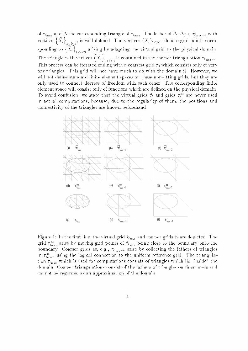
Figure �� In the rst line� the virtual grid ���max and coarser grids ��� are depicted Thegrid ���max arise by moving grid points of ���max being close to the boundary onto theboundary Coarser grids as� eg� ��max�� arise by collecting the fathers of trianglesin ���max� using the logical connection to the uniform reference grid The triangula�tion ��max which is used for computations consists of triangles which lie inside� thedomain Coarser triangulations consist of the fathers of triangles on ner levels andcannot be regarded as an approximation of the domain
�

��� The Hierarchy of Virtual Reference Grids
In this subsection� we will give the precise denition of the sequence of reference gridsIn order to indicate that a quantity belongs to the reference grid� we will use a tilde�eg� �� for the reference grid and �x for a grid point of �� The corresponding quantitieson the true triangulation are denoted by �� x� etc
The set ��� of vertices is the square grid of size �h� given by ��� � �h�Z� Wechoose an innite sequence
n�h�o�����
of step sizes with �h� � ��h��� Consequently�
we obtain that the vertex sets form a hierarchyn���
o�����
satisfying �� � ����
The corresponding hierarchy of triangulations f���g����� is given by the followingprocedure Put lines along the co�ordinate axes through the grid points of �� resulting
in a Cartesian square grid and insert diagonals through the pairs of points �h�
�m�
�
and �h�
�m� ��
�� m � Z The arising triangles dene the grid ��� �cf Figure ��a��
�c�� The triangulations ��� are nested in a natural way For any triangle �� � ����
there exist four sonsn���j
o��j��
� ������ satisfyingS�j��
���j � �� The triangle �� is the
father of each ���j� and hence� each triangle in ��� has a father in ����� provided � � �
��� Construction of the Fine Grid
Let us assume that the boundary of the domain � has to be resolved with a step width�h�max and micro�structures being smaller can be neglected Then� an intermediategrid ���max is dened by moving grid points �x � ���max of the reference grid ���max whichare close to the boundary� ie� satisfying dist ��x� ��� � h�max� together with thecorresponding edges onto the physical boundary �� This procedure denes a one�to�one mapping � � ���max � ��
�max The triangles of ���max are given by the condition�
A triangle with vertices A�B�C belongs to ���max� if and only if the triangle withvertices ��� �A� ���� �B� ���� �C� belongs to ���max
Thus� any triangle �� � ��max is linked to one and only one triangle � � ���maxThe corresponding mapping is denoted by �� � ���max � ���max Since no confusion ispossible� we skip the superscript �
The following procedure adapt illustrates� how the reference grid might be adaptedto the domain � The procedure adapt is called by
adapt����max� ���max����
��max
� ���max
��
and is dened byprocedure adapt
���� ������� �
��
Comment This routines generates the adapted triangulation � and the corres�ponding set of nodal points �
begin� �� ��� � �� �� � � �� Identity�
�

for each triangle �� of �� do begin� �� �
�����
if � � �� �� � then beginfor i � � to � do begin
Let e �� x�� x� be the ith edge of ��if e � �� �� � then begin
A� �� arg minx����e
kx� x�k for � � f�� �g �
Comment � and � are updated in the following step�if kx� �A�k � kx� �A�k then x� �� A� else x� �� A��Comment � is updated in the following step�� �� � ��� � �
end end end end end�The result of the procedure adapt applied to the triangulation ���max is depicted
in Figure ��d�Note that the algorithm adapt is not regarded as a subroutine in an implemen�
tation� but as a formal description of the explanations above In order to obtain thenite grid ��max which represents a proper triangulations of the domain �� we neglectall triangles� lying essentially outside of the domain
��max �n� � ���max j all vertices of � lie in ��
o
In view of this denition� it is clear� how to modify the procedure adapt such thatonly a nite number of triangles appear One should consider only those elementsof ���max which intersects the boundary and construct the corresponding elements of���max and� then� extending the triangulation over the whole interior of the domainWe skip the algorithmic details� since they will be discussed in a second part of thepaper
��� Coarsening of the Fine Grid
Since the grid ���max is linked to the reference grid ���max by the mapping �� we can usethe logical regularity of the reference grid to construct coarser grids ��� � for � �maxWe dene the mapping �� acting on triangles �� � ��� by the following conditionsLet
n�Xi
o��i��
denote the vertices of �� and Xi � ���Xi
� The triangle with vertices
fXig��i�� is denoted by � and we put � � ��
���� Since no confusion is possible�
we skip the index � and simply write � The adapted triangulation ��� are given by�cf Figure ��d���f��
��� �� � ����� ��n� j ��� ��� � ���
o
Obviously� the grids ��� consist of innitely many triangles and� hence� cannot beused for practical computations The coarser nite grids �� and the corresponding
�

sets of grid points ��� for � �max are dened recursively by
��max is dened as above�
��max consists of all vertices of ��max
Assume that ���� and ���� are given Then� �� is dened by
�� � �n� � ��� j �� � ���� � �
�� ��� is the father of ��� ����o
�� � ��� j x � ���� � x �
�
�
����
and �� is the set of all vertices of ��We will not go further into algorithmic details as� eg� the application of relaxation
strategies to the grids in order to avoid too large angles in triangles� edge swapping�the generation of coarse grid triangulations without generating the full ne grid�etc� but refer to the announced second part of this paper The main issue of thispaper lies in the denition of suitable nite element spaces for such grids and toprove the approximation property This is done in a more abstract setting� thus� theconstruction presented in procedure adapt can be regarded as an illustration howthe abstract assumptions which are made in the following chapters can be satised
� Composite Finite Element Spaces on � � R�
In this chapter� we will introduce so�called Composite Finite Element Spaces on coars�ened nite element grids We will present the adaption of the uniform� virtual ref�erence grid ���max to the true triangulation ��max in a more general setting in orderto treat adaptation strategies� possibly di�erent from that described in procedureadapt� within the same framework All nite element functions will be dened onthe grid ��max We recall that in applications ��max usually will not be the nest gridbut can be viewed as the coarsest grid where standard renement strategies applyOn the coarser grids ��� for � � � �max� we will use the nodal points to dene gridfunctions in a purely algebraic way Then� these vectors are interpolated by usingstandard nite element interpolation on �� in order to dene the corresponding gridfunction on a ner level Finally� we will get a grid function on ��max� which will beinterpreted as a nite element function by standard prolongation
The reason for separating the investigation of the case � � R� from the case of abounded domain is to avoid as much as possible technicalities in the presentation ofthe principal ideas
We consider here the approximation of functions u � H� �� H� �R�� by piecewiselinear functions For this purpose� let R� be partitioned into a hierarchy of uniformreference triangulations f���g����� as explained in the previous chapter We do notrestrict ourself to the case that the grid ��max has to be generated by the procedure
�

adapt� but assume in an abstract way that � � ���max � ���max
and �� � ��� � ���transfer the reference grid onto the true triangulation The correspondence of � and�� is the same as explained in the previous chapter Since no confusion is possible�we skip the superscript � Since the domain � � R�� it is not necessary to restrict��� to a nite triangulation �� Here� we identify ��� with �� and skip the superscript�
The triangulations f��g�����max are not physically nested However� we will denea logical hierarchy using the physical hierarchy of the reference grid For this� wehave to introduce some notations
��� Notations
Let Hs ��� denote the usual Sobolev spaces as� eg� dened in the book of Adams
�see ����� equipped with the scalar product ��� ��s�� and norm k�ks�� �q��� ��s�� The
seminorm containing only the derivatives of highest order is denoted by j�js��We have to distinguish between a set of triangles and the domain dened by the
union of these triangles For any set of triangles �� we dene dom� by
dom� ������
�
Since no confusion is possible� we write kvk�t�� instead of kvk�t�dom� On level � � k�
each reference triangle �� � ��� has �k sons characterized by the conditions
son��k�
����� ���k
dom son��k�
����� ��
Similarly� we dene the sons of a triangle � � �� on level �� k as the set
son��k� ��� �� ��son��k�
���� ���
��and as an abbreviation
� ��� � son�max� ��� ���
The sons of a triangle � are not nested in the sense that � � dom�son��k� ���
�is
true in general A hierarchical structuring is given by � ��� of ��� For all triangles� � ��� we obtain
dom��son��k� ���
�� dom� ���
anddom� ���� � dom� ��� � �� � son��k� ���
This situation is illustrated in Figure �
�

Figure �� The left picture shows the domain dom�� ���� of a triangle � � ��max���while the right one shows �
The father F ���k ��
�� of a triangle �� � ���k on coarser levels �� is dened corre�spondingly by
F ���k ��
�� � �� �� � son��k� ��� ���
Furthermore� we have to associate sets of triangles with the corresponding verticesFor any set of triangles � � ��� we dene V by
V ��� � �� � �� ���
��� Construction of Composite Finite Element Spaces
In order to dene the nite element spaces on ��� we rst have to introduce gridfunctions which are mappings � � �� � C The space of grid functions on level � isdenoted by C�
We introduce prolongation operators P ���� � C� � C��� by�
P ���� �
��x� �
�I int� �
��x� � x � �����
where the interpolation I int� � C� � C� �R�� is dened by the conditions
I int� � is a�ne on each � � ��� ����I int� �
��x� � � �x� x � ��
The prolongation operator P�� which associates to each grid function � � C� a gridfunctions on level �max� nally is dened by
P� �� P �max�max��P
�max���max�� � � �P
����
The interpolation of P� � at level �max describes the following nite element space
S� ��nv � H�
�R��j � � C� � v � I int�max
P� �o
We will illustrate this denition by characterizing the basis functions of S� Forsimplicity we choose � � �max � � Let �� denote the unit vector on ��� ie
�� �x� ��
�� if � � ��� otherwise�
�

for all nodal points x � �� The a�ne interpolant of � on the grid �� is the standardhat function �� �x� on the grid �� This function �� �x� is now used to dene the valuesof the prolonged unit vector P ���
� �� � ie ��P ���� ��
��x� � �� �x� � x � ����
Finally� the linear interpolant of P ���� �� is the basis function of S� corresponding to
the nodal point x� The situation is illustrated in Figure �
Figure �� Basisfunction of S� generated by interpolating the standard basis functionin the nodal points of the ner level
Remark � If the mapping � � ���max � ��max is the identity� then the space S� is thestandard �nite element space on the grid ���
In any case� the spaces S� are nested in the sense that Sj � Sk for k � j�
��� Localization of the Interpolation Process
By the linearity of P�� it follows that� for all � � C� � we can write
�P� �� �x� �Xy��
cy �x� � �y� ���
with some coe�cients cy �x� which are independent of � The mapping P� has to belocal in the sense that� for the computation of a value �P� �� �x�� only values � �y�are needed which correspond to grid points y lying close to x In order to give theformal denition of this� we need the following
De�nition � Let � � ��max� The set of triangles on level �� which in�uence thecomputation of f�P� �� �x�gx�V�� in ��� is given by
I� ��� �n�� � �� j y�� y� � V ���� � y� �� y�� x � V ��� � cyj �x� �� �
o ���
��
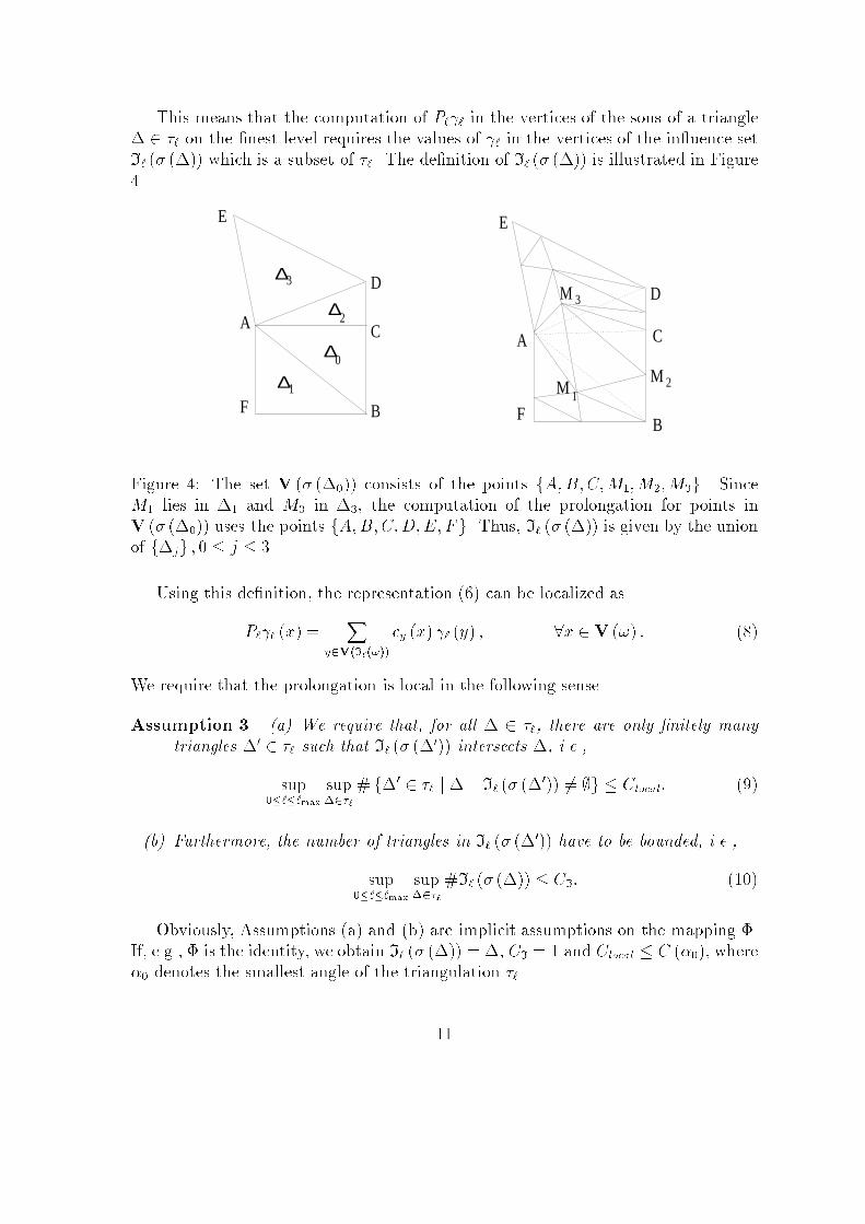
This means that the computation of P� � in the vertices of the sons of a triangle� � �� on the nest level requires the values of � in the vertices of the in uence setI� �� ���� which is a subset of �� The denition of I� �� ���� is illustrated in Figure�
A
B
C
D
E
FM 1
2
3
M
M
A
FB
C
D
E
∆
∆
∆
∆
1
3
2
0
Figure �� The set V �� ����� consists of the points fA�B�C�M��M��M�g SinceM� lies in �� and M� in ��� the computation of the prolongation for points inV �� ����� uses the points fA�B�C�D�E�Fg Thus� I� �� ���� is given by the unionof f�jg � � � j � �
Using this denition� the representation ��� can be localized as
P� � �x� �X
y�VI����
cy �x� � �y� � x � V ��� ���
We require that the prolongation is local in the following sense
Assumption � �a� We require that� for all � � ��� there are only �nitely manytriangles �� � �� such that I� �� ����� intersects �� i�e��
sup�����max
sup���
! f�� � �� j � � I� �� ����� �� �g � Clocal ���
�b� Furthermore� the number of triangles in I� �� ����� have to be bounded� i�e��
sup�����max
sup���
!I� �� ���� � CI ����
Obviously� Assumptions �a� and �b� are implicit assumptions on the mapping �If� eg� � is the identity� we obtain I� �� ���� � �� CI � � and Clocal � C ����� where�� denotes the smallest angle of the triangulation ��
��
Remark � Let v � I int� P� � and � � ��� Then the restriction v jdom��� is uniquelydetermined by the values � �x� for x � V �I� �� ������ For example� � �x� � � forall x � V �I� �� ����� implies that v jdom���� ��
The following assumption controls the regularity of the grid and the distortion oftriangles by �
Assumption � �a� Each triangle � � ������ �� has the same orientation as
�� � ����
�b� h� �� sup��� diamf�g �
�c� h� � C diamf�g � � � ��� i�e�� �� is quasiuniform� while ��� is uniform�
�d� sup fdiamS j S is a ball contained in �g � Ch�� � � ���
�e� h� � �� � Cref �h���� with ��� Cref � �
while all constants above are positive and independent of � and ��
�f� Let � � �� and � � m �max� We introduce a parameter which controls thedistortion of dom sonm��
m ���� relative to a triangle �� � Im �� ���� by
dm ��� �� max���Im����
maxx�domsonm��
m ���dist �x����
diam�� ����
We assume that � is such that for all � � ��
�max��Xm��
dm ��� � C ����
is satis�ed with a constant C independent of �� �max� and ��
Assumption ��f� can be interpreted in the following way Let � � C� denotea grid function The computation of �max �� P� � can be split by introducing localintermediate grid function m�� for � � m � �max � � by the recursion
m�� �x� �X
y�VIm�����
cy �x� m �y� � x � V �Im�� �� �����
Condition ���� controls the distortion of the triangles of Im �� ���� compared withits sons on the ner level Later� this will be used in order to prove stability ofthe interpolation process P� Some relations to typical renement strategies andimplications are concerned in the following
��

Lemma �a� If the grid ��max was constructed by the procedure adapt� then� Assumption �f� is satis�ed�
�b� Let � � �� be a triangle with an edge e � X�X� corresponding to a boundarypiece e� of class C�� Let the midpoint of e be projected onto e� by a re�nementprocedure resulting in x � e�� Then� we obtain
dist �x��� � Ch�� ����
This assumption implies ����� too��c� If Assumption �f�� is satis�ed� we get
j� ���j
j�j� C
while for any set of triangles �� j�j denotes the area measure of dom��
Proof� By the procedure adapt each grid point ���max is moved at most by a distanceof O �h�max� Let �� � ��� and �ej an edge of �� Let M
jdenote the midpoint of this
edge Then� we know thatdist
�Mj � ��
�� �
In view of ����� we have to estimate
maxx�domson���
���
dist �x��� � max��j��
dist �� �Mj� ��� � max��j��
dist �� �Mj� ����ej�� � �Ch�max
and in view of the shape regularity of the triangles� ie� Assumption ��a���e�� we getfor any � � ��
dm ��� � max���Im����
maxx�domsonm��
m ���dist �x����
diam��� C �� � Cref �
m��max
This implies that
�max��Xm��
dm ��� ��max��Xm��
C �� � Cref�m��max �
C
Cref
Estimate ���� is well known and proven by introducing a local coordinate systemwith origin in the point "x of e� having maximal distance from e and expanding e� asa Taylor series about "x Here� we skip the details It follows that in this case
dm ��� � C �� � Cref ��m � � � ��
holds and� hence��maxXm��
dm ��� ��maxX���
C �� � Cref ��� �
"C
Cref
��
In order to prove statement �c�� we proceed as follows Let �� �� � � �� and���j �� dom son��j� ��� In view of the coarsening process we know that ���j is apolygon having a boundary which consists of at most � � �j straight lines Let �� bedened by
���j �� maxx����j
dist �x� ���j���
Therefore� we can estimate
j���j��j � j���j j� � � �jh��j���j
�
Let �� �� �max � � Inductively� we obtain
j��maxj � j��j��
�
����Xj��
�jh��j���j � j�j��
�
����Xj��
�jh���j���jh��j
� j�j��
�h��
����Xj��
��
�� � Cref ��
�j���jh��j
� j�j��
�h��
��Xj��
���jh��j
�
since Cref � �� implies that �
���Cref�� � Due to the assumption on the shape
regularity of the triangles� we obtain
j��maxj � j�j
�� � C��Xj��
d��j ���
A � C j�j
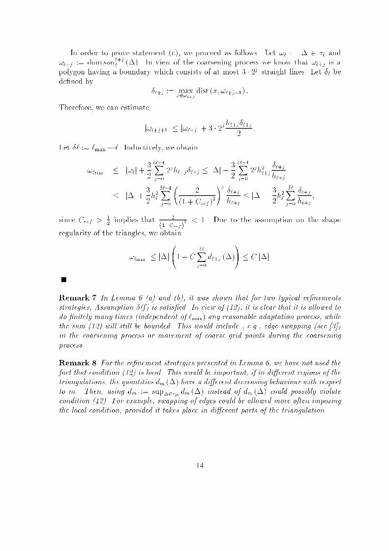
Remark In Lemma � �a� and �b�� it was shown that for two typical re�nementsstrategies� Assumption �f� is satis�ed� In view of ����� it is clear that it is allowed todo �nitely many times �independent of �max� any reasonable adaptation process� whilethe sum ���� will still be bounded� This would include � e�g�� edge swapping �see � ��in the coarsening process or movement of coarse grid points during the coarseningprocess�
Remark � For the re�nement strategies presented in Lemma �� we have not used thefact that condition ���� is local� This would be important� if in di�erent regions of thetriangulations� the quantities dm ��� have a di�erent decreasing behaviour with respectto m� Then� using dm �� sup��m dm ��� instead of dm ��� could possibly violatecondition ����� For example� swapping of edges could be allowed more often imposingthe local condition� provided it takes place in di�erent parts of the triangulation�
��

� Approximation of Functions u � H��R�
�In this chapter� we will develop the analysis of nite element approximation for func�tions v � H� �R�� Throughout this chapter� we will use the notation H t �� H t ���In Chapter � the case of a bounded domain will be discussed Here� we will developan estimate of the approximation error in the form that� for all v � H� and t � f�� �g�there exists a function v� � S� such that
kv � v�kt�R� � Ch��t� jvj��R�
The error analysis is split into the following steps For a function v � H�� we denethe restriction operator R� � C� � C� by
�R�v� �x� �� v �x� � x � �� ����
The interpolation operator on the grid �� was denoted by I int� We recall the denitionof the nodal values V �sonm� �� corresponding to the sons of � on level m �see ����Let vm be given by
vm �� I int�maxPmRmv
Using the triangle inequality� we obtain
kv � v�k������ � �
�kv � v�maxk������ �
X������
kv�max � v�k�����
A� �
�kv � v�maxk������ �
X������
maxx�V����
j�v � v�� �x�j� k�k�����
AFor the rst term on the right side above standard error estimates apply We willshow that the pointwise errors� appearing in the second term of the right hand sideabove� can be estimated by Ch� kvkI����� and hence the approximation property in
L� follows The stability of the interpolation process in H� plays the key role for theH��estimate We will show that
jv�maxj� � C jv�j�
is satised under moderate assumptions on the renement �resp coarsening� processIn combination with the L��estimate and the inverse inequality the approximationproperty in H� follows
In this light� we will assume throughout this and the following chapters thatAssumptions � and � are satised
We begin to estimate the approximation quality of S� in L�
Lemma � Let u � H� and � � C� be the interpolating grid function of u�
� �x� � u �x� � x � ��
��

Let �max � P� � be the corresponding grid function on the �nest level�Then� for all � � ��� the pointwise estimate�
j �max �x�� u �x�j � Ch� juj��I����� � x � V �� ���� ����
is satis�ed�
Proof� We dene the intermediate grid function m�� � Cm�� arising by �m� � � ���times interpolating ��
m�� �� Pm��m Pm
m�� � � �P���� �
To compute the value m�� �x� for a nodal point x � �m��� one has to determine atriangle �m � �m with x � �m The vertices of �m are denoted by fyjg��j�� Then
m�� �x� ��X
j��
�j �x� m �yj�
with some coe�cients �j �x� satisfying
�j �x� � �� � � j � �� �����X
j��
�j �x� � �
Hence� we obtain
j m�� �x�� u �x�j �
�������X
j��
�j �x� m �yj�� u �x�
�������
�������X
j��
�j �x� � m �yj�� u �yj��
��������������X
j��
�j �x�u �yj�� u �x�
�������
� �Xj��
�j �x�
A max��j��
j m �yj�� u �yj�j�
�������X
j��
�j �x�u �yj�� u �x�
������ The linear interpolant uint of u on �m in the vertices fyjg coincides with
P�j�� �j �x�u �yj�
Using standard interpolation results� we get �see ��� Theorem ������������X
j��
�j �x�u �yj�� u �x�
������ � maxx��m
juint �x�� u �x�j � Chm juj���m ����
Together� we obtain
j m�� �x�� u �x�j � max��j��
j m �yj�� u �yj�j� Chm juj���m
��

Let yk �� arg max��j�� j m �yj�� u �yj�j and yk � �m�� � �m�� The vertices of�m�� are denoted by fzjg��j�� Using the same technique as before we get
j m�� �x�� u �x�j � max��j��
j m�� �zj�� u �zj�j� Chm�� juj���m�� � Chm juj���m
Since � �x� � u �x� for all x � ��� we get inductively
j �max �x�� u �x�j � C�max��Xm��
hm juj���m
It follows that
j �max �x�� u �x�j � C juj��I�����
�maxXm��
hm � h�C
Cref
juj��I����� � x � V �� ����
with Cref dened in Assumption �Using this Lemma� we easily obtain the L��estimate of the approximation of a
H��function by interpolation
Theorem � Let v � H�� Then� there exists a function v� � S� such that
kv � v�k��R� � CClocalh�� jvj��R�
is satis�ed�
Proof� Let v � H� and � denote the interpolating grid function�
� �x� � v �x� � x � �� ����
In order to dene the corresponding nite element function� we rst have to prolong � onto the nest grid level�
�max �� P� � ����
and then to interpolate� v� �� I int�max �max The global norm can be decomposed into
local norms dened over the patches dom� ��� �
kv � v�k���R� �
X���
kv � v�k������
In the following we will use the convention thatXj��
��X
j supp j�����
This means that fj � �g denotes the indices of the vertices of � We obtain
kv � v�k������ �
X������
kv � v�k�����
� �X
������
������v �Xj���
v �xj��j �x�
�������
����
� �X
������
������Xj���
�v �xj�� v� �xj���j �x�
�������
����
��

The functionP
j��� v �xj��j �x� denotes the linear interpolant of v on �� Thereforewe know �see ��� Theorem ����� that������v �
Xj���
v �xj��j �x�
����������
� Ch��max jvj����
is fullled Using the fact that v� �x� � �max �x� for all nodal points on the nestlevel �see ����� and the pointwise estimate of the Lemma above� we conclude with
kv � v�k������ � �
X������
C�h��max jvj����� � �
X������
maxj���
j �max �xj�� v �xj�j� k�k�����
� �C�h��max jvj������ � �
X������
C�h�� jvj���I����� k�k
�����
� �C�h��max jvj������ � �C�h�� jvj
���I����� k�k
������
� "C�h�� jvj���I�����
For the last estimate we have used Lemma � �c� The global estimate follows from
kv � v�k���R� �
X���
kv � v�k������ � C�h��
X���
jvj���I�����
� C�C�localh
�� jvj
���R�
The estimate of the error in the H� seminorm is more involved The reason is thefollowing Let ��� � P ���
� � Let x � ���� and x � � � �� Then� we obtain
��� �x� �X
y�vertex of �
�y �x� � �y� �
and in view of ����� we obtain
j ��� �x�j � maxy�vertex of �
� �y�
Thus� the prolongation operator P� is stable in the maximum norm with constant� For the gradients of the interpolation ��� this is not true For j � f�� �g� letv��j � I int��j ��j and �� � son���� ��� N ��� denotes the set of neighbouring trianglesof � We will prove the representation
rv��j j���X
���N ���
���� ��rv� j ���
where the singular values of the � � � matrices ���� �� are smaller than one andP���N ���
���� �� � I Unfortunately� an estimate of the form
krv��j j��k � max���N ���
krv� j ��k
��

is not true for all grid functions � � C� Under reasonable assumption we canstill prove stability of P� in the maximum norm� but� since it is rather technical� wepostpone the proof to the Appendix The assertion is stated in the following
Lemma �� For any � and any grid function � � C� � the estimate���I intm Pmm��P
m��m�� � � �P
���� �
�����R�
� C���I int� �
�����R�
� � � m � �max
is satis�ed with a constant independent of � and �� i�e�� the interpolation process Pm
is stable in H��
Using this Lemma� the proof of the approximation property of S� is straightfor�ward
Theorem �� Let v � H�� Then� there is a function p � S� such that
jv � pj��R� � Ch� jvj��R� �
Proof� For a function v � H�� we set vm �� I int�maxPmRmv �cf ����� We will show
that the interpolant p � v� has the asserted approximation property We know that
jv � v�j��R� � jv � v�maxj��R� � jv� � v�maxj��R�
� jv � v�maxj��R� ��max��Xm��
jvm � vm��j��R� ����
Since v�max is the interpolant of v on the grid ��max� we can apply the standard niteelement estimate �see eg ��� Theorem ����� and obtain
jv � v�maxj��R� � Ch�max jvj��R�
We know that �m�� �� vm � vm�� belongs to Sm�� Let m�� � Cm�� be thecorresponding grid function�
m�� �x� � �vm � vm��� �x� � x � �m��
and �intm�� �� I intm�� m�� the interpolant on the grid �m�� Using Lemma ��� we obtain
j�m��j��R� � C����intm��
�����R�
����
We know that�intm�� �x� � �� x � �m
Similarly as in the proof of Lemma �� we will show that for each triangle � � �m theestimate ����intm�� �x�
��� � Chm jvj��I����� � x � V�sonm��
m ����
����
��

holds For this� let x � V �sonm��m ���� Then����intm�� �x�
��� � jvm �x�� vm�� �x�j � jvm �x�� v �x�j
and ���� follows from Lemma � Since the triangulation �m was assumed to be quasi�uniform� we obtain for each � � �m �
max���sonm��
m ��
���r�intm�� j����� � Ch��m��
����intm��
���L��sonm��
m ���
� Chmhm��
jvj��I����� �"C jvj��I�����
It follows that ����intm��
������R�
�X��m
X���sonm��
m ��
����intm��
��������
�X��m
X���sonm��
m ��
���r�intm�� j������ j��j
�X��m
C jvj���I�����
���dom sonm��m ���
���� CC�
localh�m jvj
���R� ����
For the last estimate� we have used Lemma � �c� Combining ����� ����� and �����we get
jv � v�j��R� � jv � v�maxj��R� ��max��Xm��
jvm � vm��j��R�
� Chmax jvj��R� � CClocal jvj��R��max��Xm��
hm
� CClocal
Cref
h� jvj��R� �
yielding the proof
� Composite Finite Element Spaces on Bounded
Domains
In this chapter� we will dene Composite Finite Element Spaces S� on bounded do�mains We will prove that� for any function u � H� ���� there is a function u� suchthat
ku� u�kt�� � Ch��t� kuk���
��

is satised for t � f�� �g The denition of the spaces will rely on a proper restrictionof the adapted grids f��g which contains innitely many triangles to the domain �
Let ��� denote the reference square grid triangulation as explained in Chapter �We recall that the mapping �� dened in Chapter �� adapts the grid points andreference grid ���max onto the intermediate grid points ��
�maxand triangulation ���max
The triangulation ��max was dened by restricting ���max to the nite domain � Thecoarser triangualtion �� were constructed by using the logical structure of the referencetriangulation �see ���� The domains corresponding to the triangulation �� are givenby
�� �� dom ��
We assume here for simplicity that � � ��max Since we assumed that ��max is suf�ciently close to �� we can treat the general case� namely� that � �� ��max with thestandard theory of nite elements on domains with curved boundary
Since the extremal points of the polygon �� are a subset of ��� condition ���guarantees that
�� � �� � � ��max � � ����
The nite element space is again dened by a suitable prolongation of grid functionsIn the case of bounded domains� the space of grid functions consists of all mappings � � �� � C� ie� � � C� � where �� is now a nite set The prolongation operatorP ���� � C� � C��� is given by
P ���� � �x� �� I int� � �x� � x � ����� ����
where I int� is the standard nite element interpolation on the �nite� grid �� Due tocondition ���� it is guaranteed that for all x � ����� there exists a triangle � � ��such that x � �� Hence� the interpolation process ���� is well dened Again� weset P� �� P �max
�max��P�max���max�� � � �P
���� The space of composite nite elements on bounded
domains is dened by
S� ��nv � R� � C j � � C� � v � I int� P� �
o
Remark �� The dimension of the space S� is given by
dimS� � !��
In the following� we will show that for every function in H� ���� there existsa function in S� which satises the asymptotic approximation property This caneasily be done by an extension argument and applying the theorems of Chapter �The following theorem concerns the existence of an extension operator for functionsu � H� ���
��

Theorem �� Let � be a domain with Lipschitz boundary� Then� there exists anextension operator E and a constant C independent of � with the property that for all� � � � �max and u � H� ��� �
uext � � Eu � �� � C�
uext j � � u j��
kuextk����� C kuk���
Proof� The proof of this theorem is given in the book of Stein ���� p���� Theorem��
The extension theorem is used to construct a function in S� having the requiredapproximation property
Theorem �� Let � be a domain with Lipschitz boundary and u � H� ���� Then�there exists a function u� � S� such that
ku� u�kt�� � Ch��t� kuk���
is satis�ed for t � f�� �g�
Proof� Let u � H� ��� and the extension uext dened as explained above Since theinclusion ���� holds� we can dene a grid function � � C� by
� �x� � uext �x� � x � ��
and u� �� I int�maxP� � the corresponding nite element function All estimates in the
case of � � R� which have been derived in the previous chapter were local in thesense that the error on patch � ��� was bounded by the H��seminorm in a localneighbourhood of � If we replace � ��� by � ��� � ��max� the theorems of Chapter� directly apply yielding
kuext � u�kt�� � Ch��t� kuextk����
for t � f�� �g Using the fact that uext j�� u j� and the continuity of the extensionoperator� we get
ku� u�kt�� � Ch��t� kuk���
� Final Remarks
In this paper� we have developed Composite Finite Elements in two dimensionsHowever� the modication of procedure adapt to the case of uniform tetrahedral
��
partitionings of R� is obvious� where the analysis of the approximation behaviourcan be carried over directly
On bounded domains� we have considered the approximation of functions in H�
which corresponds to the case of elliptic boundary value problems of second orderwith Neuman boundary conditions Dirichlet boundary conditions can be treatedby modifying the bilinear form using a penalty term The details can be found in��� The construction of composite nite element spaces satisfying Dirichlet boundaryconditions requires a slight modication of the prolongation operators� to ensure thatthe trial spaces are conforming subspaces of H�
� ����H� ��� The values of prolonged
grid functions at the boundary have to be set to zero Similiar modications arenecessary� if interfaces or changing boundary conditions are present The analysis ofthe approximation property has to be modied in these cases and will be presentedin a forthcoming paper
After having computed the sti�ness matrixA�max on the nest grid ��max� it is easyto derive coarser discretizations by means of the Galerkin product
A� ��P ����
��A���P
���� � ����
where�P ����
��denotes the adjoint of P ���
� with respect to a properly weighted Eu�clidean scalar product Since the prolongations were assumed to be local� the com�plexity of computing the sequence of matrices fA�g�����max � which is needed� eg�
in a multi�grid process� is O�h���max
�arithmetical operations However� the formula
���� is not the only way to compute A� We state that it is possible to compute the
matrix A� by a complexity of O�h��� �M�max
�� where M�max denotes the numbers
of grid points of ��max which have been moved by adapting the reference grid ���maxto the physical domain Typically M�max � O
�h���max
�is satised The algorithmic
details� together with a discussion of the complexity� is presented in the announcedsecond part of this paper
A On the Stability Condition of the Prolongation
Operator in H�
For the proof of the approximation property we have assumed that���I int�maxP� �
�����R�
� C���I int� �
�����R�
� � � C� ����
is satised We will proof this condition under Assumption � of Chapter � Since sometechnicalities will arise in this chapter� we will outline the principal ideas Firstly�we will investigate� how piecewise linear functions on a grid �� are distorted by theinterpolation process dened by P� Then� in a second step� we will estimate thegrowth of the gradients rI int�max
P� � relative to the gradients of I int� � dependent on
��

the distortion of the nodal points relative to the reference grid Finally� in a thirdstep� we will use Assumption � to obtain an estimate of the form ����
We have to introduce some notations� namely� the neighbours of a triangle � � ��by
N ��� �� f�� � �� j �� �� � and �� has a common edge with �g
We recall the denition of the father of a triangle on coarser levels �see ���� Let agrid function � � C� be given and v� �x� �� �I int� �� �x� denote the linear interpolanton �� We further dene
v��j �x� ���I int��jP
��j��j��P
��j����j�� � � �P
���� �
��x� ����
The gradient of v��j can be expressed by the gradients of v��j�� The details are inthe following
Lemma � Let �� � son��j��j�� ���� Then� the gradient of v��j can be written as
rv��j j��� rv��j�� j� �X
���N ��
���� �� �rv��j�� j �� �rv� j�� � ����
where ������ are ��� matrices of rank smaller than or equal to one� If �� and "� have
disjoint interior� then ���� �� � �� The largest singular value ��������
�can be estimated
as
� ������� � C
maxx�son���
���
dist �x���
diam�
Proof� The proof of the Lemma is elementary but technical and can be found in ���Appendix�
In the following� we will use the Lemma above to estimate the gradients of pro�longed grid functions We recall the denition of the in uence set I� �see ���� andrepresentation formula ��� For given � � C� � let v��j be dened by ���� and�� � ���j According to the representation formula ����� the gradients rv��j j�� canbe expressed as a linear combination of the gradients of rv��j�� on the father triangle� � F ��j��
��j ���� and the neighbouring triangles by ���� For a triangle �� � ���j � we
dene those neighbours "� � N ��� which satisfy ����� ��
�� � �
�
N ���� �n"� � N ��� j �m��
��� ���� �
o
The triangles which are used to compute rv��j are given by
C ���� � ��N ����
Hence� ���� can be rewritten as
rv��� j��� rv� j� �X
����
N ���
����� �� �rv� j �� �rv� j�� ����
This representation will be used to estimaterv��� j�� The details are in the following
��
Theorem � We use the notation of Lemma ��� For � � �� and � � m �max� letdm ��� be de�ned by ����� The function v� was given by ����� For �� � � ���� thegradients of v� on the �nest level can be estimated as
krv�max j��k ��max��Ym��
�� � �dm ���� max���I�����
krv� j ��k ����
Proof� Let � � �� and �� � son���� ��� Using ����� we obtain
krv� j��k �
�B� � X���
�
N���
������� ��
�CA krv��� j�k� X���
�
N���
������ ��
�krv��� j ��k
�
�� � � max���
�
N���
������� ��
�A max���C���
krv��� j ��k
Now� let �� � � ��� Using Lemma ��� we get by induction
krv�max j��k � �� � �d�max�� ���� max���C���
krv�max�� j ��k
� �� � �d�max�� ���� �� � �d�max�� ���� max���C���
maxb���C�������rv�max�� jb��
����
�max��Yr��
�� � �dr ���� max���I�����
krv�max�� j ��k �
since the iterated maxima appearing in the induction� namely
max���C����
maxb���C���� � � � �are by denition the maximum over a subset of the in uence set I� �� ����
In view of ����� we will assume an estimate of the form
krv��j j��k � C��j max���I�����
krv� j��k ����
with �� � son��j� ��� to estimate the H��seminorm of v��j The details are in thefollowing
Lemma �� Let us assume that � �� is true� Then�
jv��j j��son��j�
�� �"CC��j jv�j��I�����
is satis�ed�
��
Proof� Let � � �� and consider the triangles of son��j� ��� Then� we obtain
jv��j j���son��j
��� �
X���son��j
���
jrv��jj����� �
X���son��j
���
krv��j j��k� j��j
� C���j
�max
���I�����krv� j ��k
�� ���dom son��j� ������
� C���j
���dom son��j� ������ X���I�����
krv� j ��k�
� C���j
���dom son��j� ������ X���I�����
���� "���� jv�j����� Due to the quasi�uniformity of the grid� we know that
���� "���� � C�
j�j� "� � I� �� ����
In Lemma �� it was shown that Assumption � implies thatjdom son
��j
���j
j�j � C Con�sequently� we obtain
jv��j j��son��j�
�� � CC��j jv�j��I�����
An immediate consequence of this Lemma is the global estimate
Theorem �� Let � � C� be given and v�� v��j be de�ned by ����� Then�
jv��j j��R� � CClocalC��j jv�j��R� ����
Proof� This follows directly from Lemma �� with the constant Clocal dened by ���
Obviously� a su�cient condition for an estimate of the form
jv��j j��R� � C jv�j��R�
with a constant C independent of � and j is that C��j does not depend on � and jWe will show that Assumption � implies that C��j C Condition ��� of Assumption� reads
�maxX���
d� ��� � C ����
��

Let � � �� Hence�
�max��Y���
�� � �d� ���� � exp
���max��X���
log�� � � "Cd�
����� exp
���max��X���
� "Cd�
��� � e��CC
Condition ���� was guaranteed for the renement strategies presented in Lemma � andRemark �� and thus� result in the stability estimate of Theorem �� and nally� in therequired approximation property as has been worked out in the previous chapters
References
��� RA Adams Sobolev Spaces Academic Press� NY� ����
��� R E Bank and J Xu A Hierarchical Basis Multi�Grid Method for UnstructuredGrids In W Hackbusch and G Wittum� editors� Fast Solvers for Flow Problems�Proceedings of the Tenth GAMMSeminar� Kiel� Verlag Vieweg� ����
��� RE Bank and J Xu An Algorithm for Coarsening Unstructured Meshes Num�Math�� to appear
��� PG Ciarlet The �nite element method for elliptic problems North�Holland�����
��� W Hackbusch On the Multi�Grid Method Applied to Di�erence EquationsComputing� ������#���� ����
��� W Hackbusch MultiGrid Method and Applications Springer Verlag� ����
��� W Hackbusch Elliptic Di�erential Equations Springer Verlag� ����
��� W Hackbusch and SA Sauter Adaptive Composite Finite Elements for theSolution of PDEs Containing non�uniformly distributed Micro�Scales TechnicalReport ����� Math Sem� Universit$at Kiel� Germany� ����
��� W Hackbusch and SA Sauter Composite Finite Elements for the Approxima�tion of PDEs on Domains with Complicated Micro�Structures Technical Report������ Inst f Prakt Math� Universit$at Kiel� Germany� ����
���� W Hackbusch and SA Sauter A New Finite Element Approach for Prob�lems Containing Small Geometric Details Technical Report ����� LehrstuhlPraktische Mathematik� University of Kiel� Germany� ���� Submitted to theproceedings of the ENUMATH �� conference� Paris
��

���� R Kornhuber and H Yserentant Multilevel Methods for Elliptic Problems onDomains not Resolved by the Coarse Grid Contemporay Mathematics� ������#��� ����
���� VV Shaidurov Multigrid Methods for Finite Elements Kluwer Academic Pub�lishers� ����
���� G H Shortley and R Weller Numerical Solution of Laplace%s Equation J�Appl� Phys�� �����#���� ����
���� E M Stein Singular Integrals and Di�erentiability Properties of FunctionsPrinceton� University Press� Princeton� NJ� ����
��