1 turing machines and effective computability

Introduction to Analysis of Algorithms Notes on Turing MachinesCS4820 Spring 2013 Monday, April 1, 2013

These notes are adapted from [10].

1 Turing Machines and Effective Computability

In these notes we will introduce Turing machines (TMs), named after Alan Turing, who invented themin 1936. Turing machines can compute any function normally considered computable; in fact, it is quitereasonable to define computable to mean computable by a TM.

TMs were invented in the 1930s, long before real computers appeared. They came at a time when mathemati-cians were trying to come to grips with the notion of effective computation. They knew various algorithmsfor computing things effectively, but they weren’t quite sure how to define “effectively computable” in ageneral way that would allow them to distinguish between the computable and the noncomputable. Severalalternative formalisms evolved, each with its own peculiarities, in the attempt to nail down this notion:

• Turing machines (Alan Turing [20]);

• Post systems (Emil Post [12, 13]);

• µ-recursive functions (Kurt Godel [7], Jacques Herbrand);

• λ-calculus (Alonzo Church [2], Stephen C. Kleene [8]); and

• combinatory logic (Moses Schonfinkel [18], Haskell B. Curry [4]).

All of these systems embody the idea of effective computation in one form or another. They work on varioustypes of data; for example, Turing machines manipulate strings over a finite alphabet, µ-recursive functionsmanipulate the natural numbers, the λ-calculus manipulates λ-terms, and combinatory logic manipulatesterms built from combinator symbols.

However, there are natural translations between all these different types of data. For example, let {0, 1}∗denote the set of all finite-length strings over the alphabet {0, 1}. There is a simple one-to-one correspondencebetween {0, 1}∗ and the natural numbers N = {0, 1, 2, . . .} defined by

x 7→ #(1x)− 1, (1)

where #y is the natural number represented by the binary string y. Conversely, it is easy to encode justabout anything (natural numbers, λ-terms, strings in {0, 1, 2, . . . , 9}∗, trees, graphs, . . . ) as strings in{0, 1}∗. Under these natural encodings of the data, it turns out that all the formalisms above can simulateone another, so despite their superficial differences they are all computationally equivalent.

Nowadays we can take unabashed advantage of our more modern perspective and add programming languagessuch as Java or C (or idealized versions of them) to this list—a true luxury compared to what Church andGodel had to struggle with.

Of the classical systems listed above, the one that most closely resembles a modern computer is the Turingmachine. Besides the off-the-shelf model we will define below, there are also many custom variations (non-deterministic, multitape, multidimensional tape, two-way infinite tapes, and so on) that all turn out to becomputationally equivalent in the sense that they can all simulate one another.

1/26

CS4820 Spring 2013 Notes on Turing Machines 2/26

Church’s Thesis

Because these vastly dissimilar formalisms are all computationally equivalent, the common notion of com-putability that they embody is extremely robust, which is to say that it is invariant under fairly radicalperturbations in the model. All these mathematicians with their pet systems turned out to be looking atthe same thing from different angles. This was too striking to be mere coincidence. They soon came to therealization that the commonality among all these systems must be the elusive notion of effective computabil-ity that they had sought for so long. Computability is not just Turing machines, nor the λ-calculus, nor theµ-recursive functions, nor the Pascal programming language, but the common spirit embodied by them all.

Alonzo Church [3] gave voice to this thought, and it has since become known as Church’s thesis (or theChurch–Turing thesis). It is not a theorem, but rather a declaration that all these formalisms captureprecisely our intuition about what it means to be effectively computable in principle, no more and no less.Church’s thesis may not seem like such a big deal in retrospect, since by now we are thoroughly familiar withthe capabilities of modern computers; but keep in mind that at the time it was first formulated, computersand programming languages had yet to be invented. Coming to this realization was an enormous intellectualleap.

Probably the most compelling development leading to the acceptance of Church’s thesis was the Turingmachine. It was the first model that could be considered readily programmable. If someone laid one of theother systems out in front of you and declared, “This system captures exactly what we mean by effectivelycomputable,” you might harbor some skepticism. But it is hard to argue with Turing machines. One canrightly challenge Church’s thesis on the grounds that there are aspects of computation that are not addressedby Turing machines (for example, randomized or interactive computation), but no one could dispute thatthe notion of effective computability as captured by Turing machines is robust and important.

Universality and Self-Reference

One of the most intriguing aspects of these systems, and a pervasive theme in our study of them, is theidea of programs as data. Each of these programming systems is powerful enough that programs can bewritten that understand and manipulate other programs that are encoded as data in some reasonable way.For example, in the λ-calculus, λ-terms act as both programs and data; combinator symbols in combinatorylogic manipulate other combinator symbols; there is a so-called Godel numbering of the µ-recursive functionsin which each function has a number that can be used as input to other µ-recursive functions; and Turingmachines can interpret their input strings as descriptions of other Turing machines. It is not a far step fromthis idea to the notion of universal simulation, in which a universal program or machine U is constructedto take an encoded description of another program or machine M and a string x as input and perform astep-by-step simulation of M on input x. A modern-day example of this phenomenon would be a Schemeinterpreter written in Scheme.

One far-reaching corollary of universality is the notion of self-reference. It is exactly this capability that ledto the discovery of natural uncomputable problems. If you know some set theory, you can convince yourselfthat uncomputable problems must exist by a cardinality argument: there are uncountably many decisionproblems but only countably many Turing machines. However, self-reference allows us to construct verysimple and natural examples of uncomputable problems. For example, there do not exist general proceduresthat can determine whether a given block of code in a given C program is ever going to be executed, orwhether a given C program will ever halt. These are important problems that compiler builders would liketo solve; unfortunately, one can give a formal proof that they are unsolvable.

Perhaps the most striking example of the power of self-reference is the incompleteness theorem of Kurt Godel.Starting near the beginning of the twentieth century with Whitehead and Russell’s Principia Mathematica[21], there was a movement to reduce all of mathematics to pure symbol manipulation, independent ofsemantics. This was in part to understand and avoid the set-theoretic paradoxes discovered by Russelland others. This movement was advocated by the mathematician David Hilbert and became known as theformalist program. It attracted a lot of followers and fed the development of formal logic as we know ittoday. Its proponents believed that all mathematical truths could be derived in some fixed formal system,


just by starting with a few axioms and applying rules of inference in a purely mechanical way. This viewof mathematical proof is highly computational. The formal deductive system most popular at the timefor reasoning about the natural numbers, called Peano arithmetic (PA), was believed to be adequate forexpressing and deriving mechanically all true statements of number theory. The incompleteness theoremshowed that this was wrong: there exist even fairly simple statements of number theory that are true butnot provable in PA. This holds not only for PA but for any reasonable extension of it. This revelation wasa significant setback for the formalist program and sent shock waves throughout the mathematical world.

Godel proved the incompleteness theorem using self-reference. The basic observation needed here is that thelanguage of number theory is expressive enough to talk about itself and about proofs in PA. For example,one can write down a number-theoretic statement that says that a certain other number-theoretic statementhas a proof in PA, and one can reason about such statements using PA itself. Now, by a tricky argumentinvolving substitutions, one can actually construct statements that talk about whether they themselves areprovable. Godel actually constructed a sentence that said, “I am not provable.”

The consequences of universality are not only philosophical but also practical. Universality was in a sensethe germ of the idea that led to the development of computers as we know them today: the notion of astored program, a piece of software that can be read and executed by hardware. This programmability iswhat makes computers so versatile. Although it was only realized in physical form several years later, thenotion was definitely present in Turing’s theoretical work in the 1930s.

Informal Description of Turing Machines

We describe here a deterministic, one-tape Turing machine. This is the standard off-the-shelf model. Thereare many variations, apparently more powerful or less powerful but in reality not. We will consider some ofthese in §3.

A TM has a finite set of states Q, a semi-infinite tape that is delimited on the left end by an endmarker` and is infinite to the right, and a head that can move left and right over the tape, reading and writingsymbols.

` a b b a b a xy xy xy xy · · ·

%6

Q

two-way, read/write

The input string is of finite length and is initially written on the tape in contiguous tape cells snug up againstthe left endmarker. The infinitely many cells to the right of the input all contain a special blank symbol xy.

The machine starts in its start state s with its head scanning the left endmarker. In each step it reads thesymbol on the tape under its head. Depending on that symbol and the current state, it writes a new symbolon that tape cell, moves its head either left or right one cell, and enters a new state. The action it takesin each situation is determined by a transition function δ. It accepts its input by entering a special acceptstate t and rejects by entering a special reject state r. On some inputs it may run infinitely without everaccepting or rejecting, in which case it is said to loop on that input.

Formal Definition of Turing Machines

Formally, a deterministic one-tape Turing machine is a 9-tuple

M = (Q, Σ, Γ, `, xy, δ, s, t, r),

where

• Q is a finite set (the states);


• Σ is a finite set (the input alphabet);

• Γ is a finite set (the tape alphabet) containing Σ as a subset;

• xy ∈ Γ− Σ, the blank symbol;

• ` ∈ Γ− Σ, the left endmarker;

• δ : Q× Γ→ Q× Γ× {L,R}, the transition function;

• s ∈ Q, the start state;

• t ∈ Q, the accept state; and

• r ∈ Q, the reject state, r 6= t.

Intuitively, δ(p, a) = (q, b, d) means, “When in state p scanning symbol a, write b on that tape cell, movethe head in direction d, and enter state q.” The symbols L and R stand for left and right, respectively.

We restrict TMs so that the left endmarker is never overwritten with another symbol and the machine nevermoves off the tape to the left of the endmarker; that is, we require that for all p ∈ Q there exists q ∈ Q suchthat

δ(p,`) = (q,`, R). (2)

We also require that once the machine enters its accept state, it never leaves it, and similarly for its rejectstate; that is, for all b ∈ Γ there exist c, c′ ∈ Γ and d, d′ ∈ {L,R} such that

δ(t, b) = (t, c, d), δ(r, b) = (r, c′, d′). (3)

We sometimes refer to the state set and transition function collectively as the finite control.

Example 1. Here is a TM that accepts the non-context-free set {anbncn | n ≥ 0}. Informally, the machinestarts in its start state s, then scans to the right over the input string, checking that it is of the form a∗b∗c∗.It doesn’t write anything on the way across (formally, it writes the same symbol it reads). When it sees thefirst blank symbol xy, it overwrites it with a right endmarker a. Now it scans left, erasing the first c it sees,then the first b it sees, then the first a it sees, until it comes to the `. It then scans right, erasing one a,one b, and one c. It continues to sweep left and right over the input, erasing one occurrence of each letter ineach pass. If on some pass it sees at least one occurrence of one of the letters and no occurrences of another,it rejects. Otherwise, it eventually erases all the letters and makes one pass between ` and a seeing onlyblanks, at which point it accepts.

Formally, this machine has

Q = {s, q1, . . . , q10, t, r}, Σ = {a, b, c}, Γ = Σ ∪ {`, xy,a}.

There is nothing special about a; it is just an extra useful symbol in the tape alphabet. The transitionfunction δ is specified by the following table:

` a b c xy as (s,`, R) (s, a,R) (q1, b, R) (q2, c, R) (q3,a, L) −q1 − (r,−,−) (q1, b, R) (q2, c, R) (q3,a, L) −q2 − (r,−,−) (r,−,−) (q2, c, R) (q3,a, L) −

q3 (t,−,−) (r,−,−) (r,−,−) (q4, xy, L) (q3, xy, L) −q4 (r,−,−) (r,−,−) (q5, xy, L) (q4, c, L) (q4, xy, L) −q5 (r,−,−) (q6, xy, L) (q5, b, L) − (q5, xy, L) −q6 (q7,`, R) (q6, a, L) − − (q6, xy, L) −

q7 − (q8, xy, R) (r,−,−) (r,−,−) (q7, xy, R) (t,−,−)q8 − (q8, a, R) (q9, xy, R) (r,−,−) (q8, xy, R) (r,−,−)q9 − − (q9, b, R) (q10, xy, R) (q9, xy, R) (r,−,−)q10 − − − (q10, c, R) (q10, xy, R) (q3,a, L)


The symbol − in the table above means “don’t care.” The transitions for t and r are not included in thetable—just define them to be anything satisfying the restrictions (2) and (3).

Configurations and Acceptance

At any point in time, the read/write tape of the Turing machine M contains a semi-infinite string of theform yxyω, where y ∈ Γ∗ (y is a finite-length string) and xyω denotes the semi-infinite string

xy xy xy xy xy xy xy xy · · · .

(Here ω denotes the smallest infinite ordinal.) Although the string is infinite, it always has a finite represen-tation, since all but finitely many of the symbols are the blank symbol xy.

We define a configuration to be an element of Q×{yxyω | y ∈ Γ∗}×N, where N = {0, 1, 2, . . .}. A configurationis a global state giving a snapshot of all relevant information about a TM computation at some instant intime. The configuration (p, z, n) specifies a current state p of the finite control, current tape contents z, andcurrent position of the read/write head n ≥ 0. We usually denote configurations by α, β, γ.

The start configuration on input x ∈ Σ∗ is the configuration

(s, `xxyω, 0).

The last component 0 means that the machine is initially scanning the left endmarker `.

One can define a next configuration relation1−→M

. For a string z ∈ Γω, let zn be the nth symbol of z (the

leftmost symbol is z0), and let z[n/b] denote the string obtained from z by substituting b for zn at positionn. For example,

` b a a a c a b c a · · · [4/b] = ` b a a b c a b c a · · · .

The relation1−→M

is defined by

(p, z, n)1−→M

{(q, z[n/b], n− 1) if δ(p, zn) = (q, b, L),(q, z[n/b], n+ 1) if δ(p, zn) = (q, b, R).

Intuitively, if the tape contains z and if M is in state p scanning the nth tape cell, and δ says to print b,go left, and enter state q, then after that step the tape will contain z[n/b], the head will be scanning the(n− 1)st tape cell, and the new state will be q.

We define the reflexive transitive closure∗−→M

of1−→M

inductively:

• α 0−→M

α,

• α n+1−→M

β if αn−→M

γ1−→M

β for some γ, and

• α ∗−→M

β if αn−→M

β for some n ≥ 0.

The machine M is said to accept input x ∈ Σ∗ if

(s,` xxyω, 0)∗−→M

(t, y, n)

for some y and n and is said to reject x if

(s,` xxyω, 0)∗−→M

(r, y, n)


for some y and n. It is said to halt on input x if it either accepts x or rejects x. This is just a mathematicaldefinition; the machine doesn’t really grind to a halt in the literal sense. It is possible that it neither acceptsnor rejects, in which case it is said to loop on input x. A Turing machine is said to be total if it halts on allinputs; that is, if for all inputs it either accepts or rejects. The set L(M) denotes the set of strings acceptedby M .

We call a set of strings

• recursively enumerable (r.e.) if it is L(M) for some Turing machine M ,

• co-r.e. if its complement is r.e., and

• recursive if it is L(M) for some total Turing machine M .

In common parlance, the term “recursive” usually refers to an algorithm that calls itself. The definitionabove has nothing to do with this usage. As used here, it is just a name for a set accepted by a Turingmachine that always halts.

Historical Notes

Church’s thesis is often referred to as the Church–Turing thesis, although Alonzo Church was the first toformulate it explicitly [3]. The thesis was based on Church and Kleene’s observation that the λ-calculus andthe µ-recursive functions of Godel and Herbrand were computationally equivalent [3]. Church was apparentlyunaware of Turing’s work at the time of the writing of [3], or if he was, he failed to mention it. Turing, onthe other hand, cited Church’s paper [3] explicitly in [20], and apparently considered his machines to be amuch more compelling definition of computability. In an appendix to [20], Turing outlined a proof of thecomputational equivalence of Turing machines and the λ-calculus.

2 Examples of Turing Machines

In the last section we defined deterministic one-tape Turing machines:

M = (Q, Σ, Γ, `, xy, δ, s, t, r)

6states

6

input alphabet

6

tape alphabet

6

left endmarker

6

blank symbol

6

transition function

6

start state

6

accept state

6reject state

` a b b a b a xy xy xy xy · · ·

%6

Q

two-way, read/write

In each step, based on the current tape symbol it is reading and its current state, it prints a new symbol onthe tape, moves its head either left or right, and enters a new state. This action is specified formally by thetransition function

δ : Q× Γ → Q× Γ× {L,R}.

Intuitively, δ(p, a) = (q, b, d) means, “When in state p scanning symbol a, write b on that tape cell, movethe head in direction d, and enter state q.”


We defined a configuration to be a triple (p, z, n) where p is a state, z is a semi-infinite string of the formyxyω, y ∈ Σ∗, describing the contents of the tape, and n is a natural number denoting a tape head position.

The transition function δ was used to define the next configuration relation1−→M

on configurations and its

reflexive transitive closure∗−→M

. The machine M accepts input x ∈ Σ∗ if

(s,` xxyω, 0)∗−→M

(t, y, n)

for some y and n, and rejects input x if

(s,` xxyω, 0)∗−→M

(r, y, n)

for some y and n. The left configuration above is the start configuration on input x. Recall that we restrictedTMs so that once a TM enters its accept state, it may never leave it, and similarly for its reject state. If Mnever enters its accept or reject state on input x, it is said to loop on input x. It is said to halt on input xif it either accepts or rejects. A TM that halts on all inputs is called total.

Define the set

L(M) = {x ∈ Σ∗ |M accepts x}.

This is called the set accepted by M . A subset of Σ∗ is called recursively enumerable (r.e.) if it is L(M) forsome M . A set is called recursive if it is L(M) for some total M .

For now, the terms r.e. and recursive are just technical terms describing the sets accepted by TMs and totalTMs, respectively; they have no other significance. We will discuss the origin of this terminology in §3.

Example 2. Consider the set {ww | w ∈ {a, b}∗}, the set of all strings over the alphabet {a, b} consistingof two concatenated copies of some string w. It is a recursive set, because we can give a total TM M for it.The machine M works as follows. On input x, it scans out to the first blank symbol xy, counting the numberof symbols mod 2 to make sure x is of even length and rejecting immediately if not. It lays down a rightendmarker a, then repeatedly scans back and forth over the input. In each pass from right to left, it marksthe first unmarked a or b it sees with . In each pass from left to right, it marks the first unmarked a or b itsees with . It continues this until all symbols are marked. For example, on input

a a b b a a a b b a

the initial tape contents are`a a b b a a a b b a xy xy xy · · ·

and the following are the tape contents after the first few passes.

`a a b b a a a b b a axy xy xy · · ·` a a b b a a a b b a axy xy xy · · ·` a a b b a a a b b a axy xy xy · · ·` a a b b a a a b b a axy xy xy · · ·` a a b b a a a b b a axy xy xy · · ·

Marking a with ` formally means writing the symbol a ∈ Γ; thus

Γ = {a, b, `, xy, a, a, b, a, b}.

When all symbols are marked, we have the first half of the input string marked with ` and the second halfmarked with .

` a a b b a a a b b a axy xy xy · · ·

The reason we did this was to find the center of the input string.


The machine then repeatedly scans left to right over the input. In each pass it erases the first symbol it seesmarked with ` but remembers that symbol in its finite control (to “erase” really means to write the blanksymbol xy). It then scans forward until it sees the first symbol marked with , checks that that symbol is thesame, and erases it. If the two symbols are not the same, it rejects. Otherwise, when it has erased all thesymbols, it accepts. In our example, the following would be the tape contents after each pass.

a a b b a a a b b a axy xy xy · · ·xy a b b a xy a b b a axy xy xy · · ·xy xy b b a xy xy b b a axy xy xy · · ·xy xy xy b a xy xy xy b a axy xy xy · · ·xy xy xy xy a xy xy xy xy a axy xy xy · · ·xy xy xy xy xy xy xy xy xy xy axy xy xy · · ·

Example 3. We want to construct a total TM that accepts its input string if the length of the string isprime. We will give a TM implementation of the sieve of Eratosthenes, which can be described informally asfollows. Say we want to check whether n is prime. We write down all the numbers from 2 to n in order, thenrepeat the following: find the smallest number in the list, declare it prime, then cross off all multiples of thatnumber. Repeat until each number in the list has been either declared prime or crossed off as a multiple ofa smaller prime.

For example, to check whether 23 is prime, we would start with all the numbers from 2 to 23:

2 3 4 5 6 7 8 9 10 11 12 13 14 15 16 17 18 19 20 21 22 23

In the first pass, we cross off multiples of 2:

2 3 4 5 6 7 8 9 10 11 12 13 14 15 16 17 18 19 20 21 22 23� � � �@ @ @ @ � � � � � � �@ @ @ @ @ @ @

The smallest number remaining is 3, and this is prime. In the second pass we cross off multiples of 3:

2 3 4 5 6 7 8 9 10 11 12 13 14 15 16 17 18 19 20 21 22 23� � � �@ @ @ @ � � � � � � �@ @ @ @ @ @ @� �@ @ � �@ @

Then 5 is the next prime, so we cross off multiples of 5; and so forth. Since 23 is prime, it will never becrossed off as a multiple of anything smaller, and eventually we will discover that fact when everythingsmaller has been crossed off.

Now we show how to implement this on a TM. Suppose we have ap written on the tape. We illustrate thealgorithm with p = 23.

`a a a a a a a a a a a a a a a a a a a a a a a xy xy xy · · ·If p = 0 or p = 1, reject. We can determine this by looking at the first three cells of the tape. Otherwise,there are at least two a’s. Erase the first a, scan right to the end of the input, and replace the last a in theinput string with the symbol $. We now have an a in positions 2, 3, 4, . . . , p− 1 and $ at position p.

`xy a a a a a a a a a a a a a a a a a a a a a $ xy xy xy · · ·

Now we repeat the following loop. Starting from the left endmarker `, scan right and find the first nonblanksymbol, say occurring at position m. Then m is prime (this is an invariant of the loop). If this symbol isthe $, we are done: p = m is prime, so we halt and accept. Otherwise, the symbol is an a. Mark it with a and everything between there and the left endmarker with .

` xy a a a a a a a a a a a a a a a a a a a a a $ xy xy xy · · ·

We will now enter an inner loop to erase all the symbols occurring at positions that are multiples of m.First, erase the a under the . (Formally, just write the symbol xy.)

` xy xy a a a a a a a a a a a a a a a a a a a a $ xy xy xy · · ·

Shift the marks to the right one at a time a distance equal to the number of marks. This can be done byshuttling back and forth, erasing marks on the left and writing them on the right. We know when we aredone because the is the last mark moved.

`xy xy a a a a a a a a a a a a a a a a a a a a $ xy xy xy · · ·


When this is done, erase the symbol under the . This is the symbol occurring at position 2m.

`xy xy a xy a a a a a a a a a a a a a a a a a a $ xy xy xy · · ·

Keep shifting the marks and erasing the symbol under the in this fashion until we reach the end.

`xy xy a xy a xy a xy a xy a xy a xy a xy a xy a xy a xy $ xy xy xy · · ·

If we find ourselves at the end of the string wanting to erase the $, reject—p is a multiple of m but not equalto m. Otherwise, go back to the left and repeat. Find the first nonblank symbol and mark it and everythingto its left.

` xy xy a xy a xy a xy a xy a xy a xy a xy a xy a xy a xy $ xy xy xy · · ·Alternately erase the symbol under the and shift the marks until we reach the end of the string.

`xy xy xy xy a xy a xy xy xy a xy a xy xy xy a xy a xy xy xy $ xy xy xy · · ·

Go back to the left and repeat.

` xy xy xy xy a xy a xy xy xy a xy a xy xy xy a xy a xy xy xy $ xy xy xy · · ·

If we ever try to erase the $, reject—p is not prime. If we manage to erase all the a’s, accept.

Recursive and R.E. Sets

Recall that a set A is recursively enumerable (r.e.) if it is accepted by a TM and recursive if it is acceptedby a total TM (one that halts on all inputs).

The recursive sets are closed under complement. (The r.e. sets are not, as we will see later.) That is, if Ais recursive, then so is ∼A = Σ∗ − A. To see this, suppose A is recursive. Then there exists a total TM Msuch that L(M) = A. We can build a new machine M ′ that is exactly like M except that the accept stateof M ′ is the reject state of M and the reject state of M ′ is the accept state of M . By switching accept andreject states, we get a total machine M ′ such that L(M ′) = ∼A.

This construction does not give the complement if M is not total. This is because “rejecting” and “notaccepting” are not synonymous for nontotal machines. To reject, a machine must enter its reject state. IfM ′ is obtained from M by just switching the accept and reject states, then M ′ will accept the strings thatM rejects and reject the strings that M accepts; but M ′ will still loop on the same strings that M loops on,so these strings are not accepted or rejected by either machine.

Every recursive set is r.e. but not necessarily vice versa. In other words, not every TM is equivalent to atotal TM. We will prove this in §4. However, if both A and ∼A are r.e., then A is recursive. To see this,suppose both A and ∼A are r.e. Let M and M ′ be TMs such that L(M) = A and L(M ′) = ∼A. Builda new machine N that on input x runs both M and M ′ simultaneously on two different tracks of its tape.Formally, the tape alphabet of N contains symbols

c

a

c

a

c

a

c

a

where a is a tape symbol of M and c is a tape symbol of M ′. Thus N ’s tape may contain a string of theform

c

b

c

a

c

b

d

a

d

b

c

a

c

b

d

a · · ·

for example. The extra marks are placed on the tape to indicate the current positions of the simulatedread/write heads of M and M ′. The machine N alternately performs a step of M and a step of M ′, shuttlingback and forth between the two simulated tape head positions of M and M ′ and updating the tape. Thecurrent states and transition information of M and M ′ can be stored in N ’s finite control. If the machineM ever accepts, then N immediately accepts. If M ′ ever accepts, then N immediately rejects. Exactly oneof those two events must eventually occur, depending on whether x ∈ A or x ∈ ∼A, since L(M) = A andL(M ′) = ∼A. Then N halts on all inputs and L(N) = A.


Decidability and Semidecidability

A property P of strings is said to be decidable if the set of all strings having property P is a recursive set;that is, if there is a total Turing machine that accepts input strings that have property P and rejects thosethat do not. A property P is said to be semidecidable if the set of strings having property P is an r.e. set;that is, if there is a Turing machine that on input x accepts if x has property P and rejects or loops if not.For example, it is decidable whether a given string x is of the form ww, because we can construct a Turingmachine that halts on all inputs and accepts exactly the strings of this form.

Although you often hear them switched, the adjectives recursive and r.e. are best applied to sets anddecidable and semidecidable to properties. The two notions are equivalent, since

P is decidable ⇔ {x | P (x)} is recursive.

A is recursive ⇔ “x ∈ A” is decidable,

P is semidecidable ⇔ {x | P (x)} is r.e.,

A is r.e. ⇔ “x ∈ A” is semidecidable.

3 Equivalent Models

As mentioned, the concept of computability is remarkably robust. As evidence of this, we will present severaldifferent flavors of Turing machines that at first glance appear to be significantly more or less powerful thanthe basic model defined in §2 but in fact are computationally equivalent.

Multiple Tapes

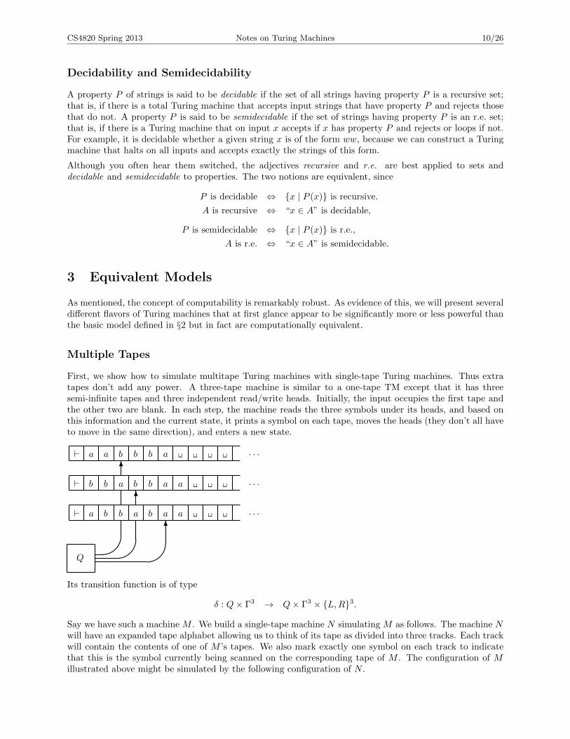
First, we show how to simulate multitape Turing machines with single-tape Turing machines. Thus extratapes don’t add any power. A three-tape machine is similar to a one-tape TM except that it has threesemi-infinite tapes and three independent read/write heads. Initially, the input occupies the first tape andthe other two are blank. In each step, the machine reads the three symbols under its heads, and based onthis information and the current state, it prints a symbol on each tape, moves the heads (they don’t all haveto move in the same direction), and enters a new state.

` a b b a b a a xy xy xy · · ·

` b b a b b a a xy xy xy · · ·

` a a b b b a xy xy xy xy · · ·

%%%

6

6

6

Q

Its transition function is of type

δ : Q× Γ3 → Q× Γ3 × {L,R}3.

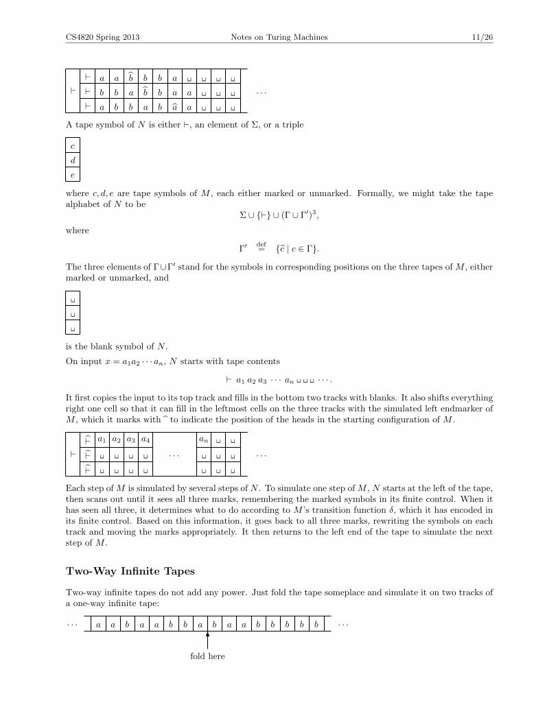
Say we have such a machine M . We build a single-tape machine N simulating M as follows. The machine Nwill have an expanded tape alphabet allowing us to think of its tape as divided into three tracks. Each trackwill contain the contents of one of M ’s tapes. We also mark exactly one symbol on each track to indicatethat this is the symbol currently being scanned on the corresponding tape of M . The configuration of Millustrated above might be simulated by the following configuration of N .


`` a b b a b a a xy xy xy

` b b a b b a a xy xy xy · · ·` a a b b b a xy xy xy xy

A tape symbol of N is either `, an element of Σ, or a triple

e

d

c

where c, d, e are tape symbols of M , each either marked or unmarked. Formally, we might take the tapealphabet of N to be

Σ ∪ {`} ∪ (Γ ∪ Γ′)3,

where

Γ′def= {c | c ∈ Γ}.

The three elements of Γ∪Γ′ stand for the symbols in corresponding positions on the three tapes of M , eithermarked or unmarked, and

xy

xy

xy

is the blank symbol of N .

On input x = a1a2 · · · an, N starts with tape contents

` a1 a2 a3 · · · an xy xy xy · · · .

It first copies the input to its top track and fills in the bottom two tracks with blanks. It also shifts everythingright one cell so that it can fill in the leftmost cells on the three tracks with the simulated left endmarker ofM , which it marks with to indicate the position of the heads in the starting configuration of M .

` a1 a2 a3 a4

· · ·

an xy xy xy xy xy xy xy xy xy · · ·

xy xy xy xy xy xy xy

Each step of M is simulated by several steps of N . To simulate one step of M , N starts at the left of the tape,then scans out until it sees all three marks, remembering the marked symbols in its finite control. When ithas seen all three, it determines what to do according to M ’s transition function δ, which it has encoded inits finite control. Based on this information, it goes back to all three marks, rewriting the symbols on eachtrack and moving the marks appropriately. It then returns to the left end of the tape to simulate the nextstep of M .

Two-Way Infinite Tapes

Two-way infinite tapes do not add any power. Just fold the tape someplace and simulate it on two tracks ofa one-way infinite tape:

· · · a a b a a b b a b a a b b b b b · · ·6

fold here


`a b b a a b a a

b a a b b b b b· · ·

The bottom track is used to simulate the original machine when its head is to the right of the fold, and thetop track is used to simulate the machine when its head is to the left of the fold, moving in the oppositedirection.

Two Stacks

A machine with a two-way, read-only input head and two stacks is as powerful as a Turing machine. Intu-itively, the computation of a one-tape TM can be simulated with two stacks by storing the tape contentsto the left of the head on one stack and the tape contents to the right of the head on the other stack. Themotion of the head is simulated by popping a symbol off one stack and pushing it onto the other. Forexample,

` a b a a b a b b b b b b b a a a b · · ·6

is simulated by

` a b a a b a b b b

6

stack 1

b b b b a a a b a6

stack 2

Counter Automata

A k-counter automaton is a machine equipped with a two-way read-only input head and k integer counters.Each counter can store an arbitrary nonnegative integer. In each step, the automaton can independentlyincrement or decrement its counters and test them for 0 and can move its input head one cell in eitherdirection. It cannot write on the tape.

A stack can be simulated with two counters as follows. We can assume without loss of generality that thestack alphabet of the stack to be simulated contains only two symbols, say 0 and 1. This is because we canencode finitely many stack symbols as binary numbers of fixed length, say m; then pushing or popping onestack symbol is simulated by pushing or popping m binary digits. Then the contents of the stack can beregarded as a binary number whose least significant bit is on top of the stack. The simulation maintainsthis number in the first of the two counters and uses the second to effect the stack operations. To simulatepushing a 0 onto the stack, we need to double the value in the first counter. This is done by entering a loopthat repeatedly subtracts one from the first counter and adds two to the second until the first counter is 0.The value in the second counter is then twice the original value in the first counter. We can then transferthat value back to the first counter, or just switch the roles of the two counters. To push 1, the operation isthe same, except the value of the second counter is incremented once at the end. To simulate popping, weneed to divide the counter value by two; this is done by decrementing one counter while incrementing theother counter every second step. Testing the parity of the original counter contents tells whether a simulated1 or 0 was popped.

Since a two-stack machine can simulate an arbitrary TM, and since two counters can simulate a stack, itfollows that a four-counter automaton can simulate an arbitrary TM.

However, we can do even better: a two-counter automaton can simulate a four-counter automaton. Whenthe four-counter automaton has the values i, j, k, ` in its counters, the two-counter automaton will have thevalue 2i3j5k7` in its first counter. It uses its second counter to effect the counter operations of the four-counter automaton. For example, if the four-counter automaton wanted to add one to k (the value of the


third counter), then the two-counter automaton would have to multiply the value in its first counter by 5.This is done in the same way as above, adding 5 to the second counter for every 1 we subtract from thefirst counter. To simulate a test for zero, the two-counter automaton has to determine whether the valuein its first counter is divisible by 2, 3, 5, or 7, respectively, depending on which counter of the four-counterautomaton is being tested.

Combining these simulations, we see that two-counter automata are as powerful as arbitrary Turing machines.However, as you can imagine, it takes an enormous number of steps of the two-counter automaton to simulateone step of the Turing machine.

One-counter automata are not as powerful as arbitrary TMs.

Enumeration Machines

We defined the recursively enumerable (r.e.) sets to be those sets accepted by Turing machines. The termrecursively enumerable comes from a different but equivalent formalism embodying the idea that the elementsof an r.e. set can be enumerated one at a time in a mechanical fashion.

Define an enumeration machine as follows. It has a finite control and two tapes, a read/write work tapeand a write-only output tape. The work tape head can move in either direction and can read and write anyelement of Γ. The output tape head moves right one cell when it writes a symbol, and it can only writesymbols in Σ. There is no input and no accept or reject state. The machine starts in its start state withboth tapes blank. It moves according to its transition function like a TM, occasionally writing symbols onthe output tape as determined by the transition function. At some point it may enter a special enumerationstate, which is just a distinguished state of its finite control. When that happens, the string currently writtenon the output tape is said to be enumerated. The output tape is then automatically erased and the outputhead moved back to the beginning of the tape (the work tape is left intact), and the machine continues fromthat point. The machine runs forever. The set L(E) is defined to be the set of all strings in Σ∗ that areever enumerated by the enumeration machine E. The machine might never enter its enumeration state, inwhich case L(E) = ∅, or it might enumerate infinitely many strings. The same string may be enumeratedmore than once.

Enumeration machines and Turing machines are equivalent in computational power:

Theorem 1. The family of sets enumerated by enumeration machines is exactly the family of r.e. sets. Inother words, a set is L(E) for some enumeration machine E if and only if it is L(M) for some Turingmachine M .

Proof. We show first that given an enumeration machine E, we can construct a Turing machine M such thatL(M) = L(E). Let M on input x copy x to one of three tracks on its tape, then simulate E, using the othertwo tracks to record the contents of E’s work tape and output tape. For every string enumerated by E, Mcompares this string to x and accepts if they match. Then M accepts its input x iff x is ever enumerated byE, so the set of strings accepted by M is exactly the set of strings enumerated by E.

Conversely, given a TM M , we can construct an enumeration machine E such that L(E) = L(M). We wouldlike E somehow to simulate M on all possible strings in Σ∗ and enumerate those that are accepted.

Here is an approach that doesn’t quite work. The enumeration machine E writes down the strings in Σ∗one by one on the bottom track of its work tape in some order. For every input string x, it simulates M oninput x, using the top track of its work tape to do the simulation. If M accepts x, E copies x to its outputtape and enters its enumeration state. It then goes on to the next string.

The problem with this procedure is that M might not halt on some input x, and then E would be stucksimulating M on x forever and would never move on to strings later in the list (and it is impossible todetermine in general whether M will ever halt on x, as we will see in §4). Thus E should not just list thestrings in Σ∗ in some order and simulate M on those inputs one at a time, waiting for each simulation tohalt before going on to the next, because the simulation might never halt.

The solution to this problem is timesharing. Instead of simulating M on the input strings one at a time,


the enumeration machine E should run several simulations at once, working a few steps on each simulationand then moving on to the next. The work tape of E can be divided into segments separated by a specialmarker # ∈ Γ, with a simulation of M on a different input string running in each segment. Between passes,E can move way out to the right, create a new segment, and start up a new simulation in that segment onthe next input string. For example, we might have E simulate M on the first input for one step, then thefirst and second inputs for one step each, then the first, second, and third inputs for one step each, and soon. If any simulation needs more space than initially allocated in its segment, the entire contents of the tapeto its right can be shifted to the right one cell. In this way M is eventually simulated on all input strings,even if some of the simulations never halt.

Historical Notes

Turing machines were invented by Alan Turing [20]. Originally they were presented in the form of enu-meration machines, since Turing was interested in enumerating the decimal expansions of computable realnumbers and values of real-valued functions. Turing also introduced the concept of nondeterminism in hisoriginal paper, although he did not develop the idea.

The basic properties of the r.e. sets were developed by Kleene [9] and Post [13, 14].

Counter automata were studied by Fischer [5], Fischer et al. [6], and Minsky [11].

4 Universal Machines and Diagonalization

A Universal Turing Machine

Now we come to a crucial observation about the power of Turing machines: there exist Turing machines thatcan simulate other Turing machines whose descriptions are presented as part of the input. There is nothingmysterious about this; it is the same as writing an OCaml interpreter in OCaml.

First we need to fix a reasonable encoding scheme for Turing machines over the alphabet {0, 1}. Thisencoding scheme should be simple enough that all the data associated with a machine M—the set of states,the transition function, the input and tape alphabets, the endmarker, the blank symbol, and the start,accept, and reject states—can be determined easily by another machine reading the encoded description ofM . For example, if the string begins with the prefix

0n10m10k10s10t10r10u10v1,

this might indicate that the machine has n states represented by the numbers 0 to n − 1; it has m tapesymbols represented by the numbers 0 to m − 1, of which the first k represent input symbols; the start,accept, and reject states are s, t, and r, respectively; and the endmarker and blank symbol are u and v,respectively. The remainder of the string can consist of a sequence of substrings specifying the transitionsin δ. For example, the substring

0p10a10q10b10

might indicate that δ contains the transition

(p, a)→ (q, b, L),

the direction to move the head encoded by the final digit. The exact details of the encoding scheme arenot important. The only requirements are that it should be easy to interpret and able to encode all Turingmachines up to isomorphism.

Once we have a suitable encoding of Turing machines, we can construct a universal Turing machine U suchthat

L(U)def= {M#x | x ∈ L(M)}.


In other words, presented with (an encoding over {0, 1} of) a Turing machine M and (an encoding over{0, 1} of) a string x over M ’s input alphabet, the machine U accepts M#x iff M accepts x.1 The symbol# is just a symbol in U ’s input alphabet other than 0 or 1 used to delimit M and x.

The machine U first checks its input M#x to make sure that M is a valid encoding of a Turing machineand x is a valid encoding of a string over M ’s input alphabet. If not, it immediately rejects.

If the encodings of M and x are valid, the machine U does a step-by-step simulation of M . This might workas follows. The tape of U is partitioned into three tracks. The description of M is copied to the top trackand the string x to the middle track. The middle track will be used to hold the simulated contents of M ’stape. The bottom track will be used to remember the current state of M and the current position of M ’sread/write head. The machine U then simulates M on input x one step at a time, shuttling back and forthbetween the description of M on its top track and the simulated contents of M ’s tape on the middle track.In each step, it updates M ’s state and simulated tape contents as dictated by M ’s transition function, whichU can read from the description of M . If ever M halts and accepts or halts and rejects, then U does thesame.

As we have observed, the string x over the input alphabet of M and its encoding over the input alphabet ofU are two different things, since the two machines may have different input alphabets. If the input alphabetof M is bigger than that of U , then each symbol of x must be encoded as a string of symbols over U ’s inputalphabet. Also, the tape alphabet of M may be bigger than that of U , in which case each symbol of M ’stape alphabet must be encoded as a string of symbols over U ’s tape alphabet. In general, each step of Mmay require many steps of U to simulate.

Diagonalization

We now show how to use a universal Turing machine in conjunction with a technique called diagonalizationto prove that the halting and membership problems for Turing machines are undecidable. In other words,the sets

HPdef= {M#x |M halts on x},

MPdef= {M#x | x ∈ L(M)}

are not recursive.

The technique of diagonalization was first used by Cantor at the end of the nineteenth century to show thatthere does not exist a one-to-one correspondence between the natural numbers N and its power set

2N = {A | A ⊆ N},

the set of all subsets of N. In fact, there does not even exist a function

f : N → 2N

that is onto. Here is how Cantor’s argument went.

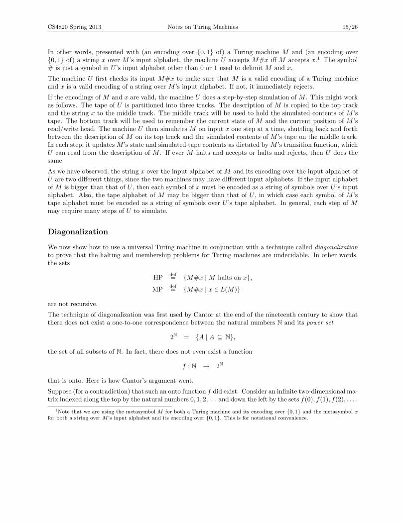
Suppose (for a contradiction) that such an onto function f did exist. Consider an infinite two-dimensional ma-trix indexed along the top by the natural numbers 0, 1, 2, . . . and down the left by the sets f(0), f(1), f(2), . . . .

1Note that we are using the metasymbol M for both a Turing machine and its encoding over {0, 1} and the metasymbol xfor both a string over M ’s input alphabet and its encoding over {0, 1}. This is for notational convenience.


Fill in the matrix by placing a 1 in position i, j if j is in the set f(i) and 0 if j 6∈ f(i).

0 1 2 3 4 5 6 7 8 9 · · ·f(0) 1 0 0 1 1 0 1 0 1 1f(1) 0 0 1 1 0 1 1 0 0 1f(2) 0 1 1 0 0 0 1 1 0 1f(3) 0 1 0 1 1 0 1 1 0 0f(4) 1 0 1 0 0 1 0 0 1 1 · · ·f(5) 1 0 1 1 0 1 1 1 0 1f(6) 0 0 1 0 1 1 0 0 1 1f(7) 1 1 1 0 1 1 1 0 1 0f(8) 0 0 1 0 0 0 0 1 1 0f(9) 1 1 0 0 1 0 0 1 0 0

......

. . .

The ith row of the matrix is a bit string describing the set f(i). For example, in the above picture,f(0) = {0, 3, 4, 6, 8, 9, . . .} and f(1) = {2, 3, 5, 6, 9, . . .}. By our (soon to be proved fallacious) assumptionthat f is onto, every subset of N appears as a row of this matrix.

But we can construct a new set that does not appear in the list by complementing the main diagonal ofthe matrix (hence the term diagonalization). Look at the infinite bit string down the main diagonal (in thisexample, 1011010010 · · · ) and take its Boolean complement (in this example, 0100101101 · · · ). This new bitstring represents a set B (in this example, B = {1, 4, 6, 7, 9, . . .}). But the set B does not appear anywherein the list down the left side of the matrix, since it differs from every f(i) on at least one element, namelyi. This is a contradiction, since every subset of N was supposed to occur as a row of the matrix, by ourassumption that f was onto.

This argument works not only for the natural numbers N, but for any set A whatsoever. Suppose (for acontradiction) there existed an onto function from A to its power set:

f : A → 2A.

Let

B = {x ∈ A | x 6∈ f(x)}

(this is the formal way of complementing the diagonal). Then B ⊆ A. Since f is onto, there must existy ∈ A such that f(y) = B. Now we ask whether y ∈ f(y) and discover a contradiction:

y ∈ f(y) ⇔ y ∈ B since B = f(y)

⇔ y 6∈ f(y) definition of B.

Thus no such f can exist.

Undecidability of the Halting Problem

We have discussed how to encode descriptions of Turing machines as strings in {0, 1}∗ so that these de-scriptions can be read and simulated by a universal Turing machine U . The machine U takes as input anencoding of a Turing machine M and a string x and simulates M on input x, and

• halts and accepts if M halts and accepts x,

• halts and rejects if M halts and rejects x, and

• loops if M loops on x.


The machine U doesn’t do any fancy analysis on the machine M to try to determine whether or not it willhalt. It just blindly simulates M step by step. If M doesn’t halt on x, then U will just go on happilysimulating M forever.

It is natural to ask whether we can do better than just a blind simulation. Might there be some way toanalyze M to determine in advance, before doing the simulation, whether M would eventually halt on x?If U could say for sure in advance that M would not halt on x, then it could skip the simulation and saveitself a lot of useless work. On the other hand, if U could ascertain that M would eventually halt on x, thenit could go ahead with the simulation to determine whether M accepts or rejects. We could then build amachine U ′ that takes as input an encoding of a Turing machine M and a string x, and

• halts and accepts if M halts and accepts x,

• halts and rejects if M halts and rejects x, and

• halts and rejects if M loops on x.

This would say that L(U ′) = L(U) = MP is a recursive set.

Unfortunately, this is not possible in general. There are certainly machines for which it is possible todetermine halting by some heuristic or other: machines for which the start state is the accept state, forexample. However, there is no general method that gives the right answer for all machines.

We can prove this using Cantor’s diagonalization technique. For x ∈ {0, 1}∗, let Mx be the Turing machinewith input alphabet {0, 1} whose encoding over {0, 1}∗ is x. (If x is not a legal description of a TM withinput alphabet {0, 1}∗ according to our encoding scheme, we take Mx to be some arbitrary but fixed TMwith input alphabet {0, 1}, say a trivial TM with one state that immediately halts.) In this way we get alist

Mε,M0,M1,M00,M01,M10,M11,M100,M101, . . . (4)

containing all possible Turing machines with input alphabet {0, 1} indexed by strings in {0, 1}∗. We makesure that the encoding scheme is simple enough that a universal machine can determine Mx from x for thepurpose of simulation.

Now consider an infinite two-dimensional matrix indexed along the top by strings in {0, 1}∗ and down theleft by TMs in the list (4).

The matrix contains an H in position x, y if Mx halts on input y and an L if Mx loops on input y.

ε 0 1 00 01 10 11 000 001 010 · · ·Mε H L L H H L H L H HM0 L L H H L H H L L HM1 L H H L L L H H L HM00 L H L H H L H H L LM01 H L H L L H L L H H · · ·M10 H L H H L H H H L HM11 L L H L H H L L H HM000 H H H L H H H L H LM001 L L H L L L L H H LM010 H H L L H L L H L L

......

. . .

The xth row of the matrix describes for each input string y whether or not Mx halts on y. For example, inthe above picture, Mε halts on inputs ε, 00, 01, 11, 001, 010, . . . and does not halt on inputs 0, 1, 10, 000, . . . .

Suppose (for a contradiction) that there existed a total machine K accepting the set HP; that is, a machinethat for any given x and y could determine the x, yth entry of the above table in finite time. Thus on inputM#x,


• K halts and accepts if M halts on x, and

• K halts and rejects if M loops on x.

Consider a machine N that on input x ∈ {0, 1}∗

(i) constructs Mx from x and writes Mx#x on its tape;

(ii) runs K on input Mx#x, accepting if K rejects and going into a trivial loop if K accepts.

Note that N is essentially complementing the diagonal of the above matrix. Then for any x ∈ {0, 1}∗,

N halts on x ⇔ K rejects Mx#x definition of N

⇔ Mx loops on x assumption about K.

This says that N ’s behavior is different from every Mx on at least one string, namely x. But the list(4) was supposed to contain all Turing machines over the input alphabet {0, 1}, including N . This is acontradiction.

The fallacious assumption that led to the contradiction was that it was possible to determine the entries ofthe matrix effectively; in other words, that there existed a Turing machine K that given M and x coulddetermine in a finite time whether or not M halts on x.

One can always simulate a given machine on a given input. If the machine ever halts, then we will know thiseventually, and we can stop the simulation and say that it halted; but if not, there is no way in general tostop after a finite time and say for certain that it will never halt.

Undecidability of the Membership Problem

The membership problem is also undecidable. We can show this by reducing the halting problem to it.In other words, we show that if there were a way to decide membership in general, we could use this as asubroutine to decide halting in general. But we just showed above that halting is undecidable, so membershipmust be undecidable too.

Here is how we would use a total TM that decides membership as a subroutine to decide halting. Given amachine M and input x, suppose we wanted to find out whether M halts on x. Build a new machine Nthat is exactly like M , except that it accepts whenever M would either accept or reject. The machine N canbe constructed from M simply by adding a new accept state and making the old accept and reject statestransfer to this new accept state. Then for all x, N accepts x iff M halts on x. The membership problemfor N and x (asking whether x ∈ L(N)) is therefore the same as the halting problem for M and x (askingwhether M halts on x). If the membership problem were decidable, then we could decide whether M haltson x by constructing N and asking whether x ∈ L(N). But we have shown above that the halting problemis undecidable, therefore the membership problem must also be undecidable.

5 Decidable and Undecidable Problems

Here are some examples of decision problems involving Turing machines. Is it decidable whether a givenTuring machine

(a) has at least 481 states?

(b) takes more than 481 steps on input ε?

(c) takes more than 481 steps on some input?

(d) takes more than 481 steps on all inputs?


(e) ever moves its head more than 481 tape cells away from the left endmarker on input ε?

(f) accepts the null string ε?

(g) accepts any string at all?

(h) accepts every string?

(i) accepts a finite set?

(j) accepts a recursive set?

(k) is equivalent to a Turing machine with a shorter description?

Problems (a) through (e) are decidable and problems (f) through (k) are undecidable (proofs below). Wewill show that problems (f) through (j) are undecidable by showing that a decision procedure for one ofthese problems could be used to construct a decision procedure for the halting problem, which we knowis impossible. Problem (k) is a little more difficult, and we will leave that as an exercise. Translated intomodern terms, problem (k) is the same as determining whether there exists a shorter Java program equivalentto a given one.

The best way to show that a problem is decidable is to give a total Turing machine that accepts exactly the“yes” instances. Because it must be total, it must also reject the “no” instances; in other words, it must notloop on any input.

Problem (a) is easily decidable, since the number of states of M can be read off from the encoding of M .We can build a Turing machine that, given the encoding of M written on its input tape, counts the numberof states of M and accepts or rejects depending on whether the number is at least 481.

Problem (b) is decidable, since we can simulate M on input ε with a universal machine for 481 steps (countingup to 481 on a separate track) and accept or reject depending on whether M has halted by that time.

Problem (c) is decidable: we can just simulate M on all inputs of length at most 481 for 481 steps. If Mtakes more than 481 steps on some input, then it will take more than 481 steps on some input of length atmost 481, since in 481 steps it can read at most the first 481 symbols of the input.

The argument for problem (d) is similar. If M takes more than 481 steps on all inputs of length at most481, then it will take more than 481 steps on all inputs.

For problem (e), if M never moves more than 481 tape cells away from the left endmarker, then it will eitherhalt or loop in such a way that we can detect the looping after a finite time. This is because if M has k statesand m tape symbols, and never moves more than 481 tape cells away from the left endmarker, then thereare only 482km481 configurations it could possibly ever be in, one for each choice of head position, state,and tape contents that fit within 481 tape cells. If it runs for any longer than that without moving morethan 481 tape cells away from the left endmarker, then it must be in a loop, because it must have repeated aconfiguration. This can be detected by a machine that simulates M , counting the number of steps M takeson a separate track and declaring M to be in a loop if the bound of 482km481 steps is ever exceeded.

Problems (f) through (j) are undecidable. To show this, we show that the ability to decide any one ofthese problems could be used to decide the halting problem. Since we know that the halting problem isundecidable, these problems must be undecidable too. This is called a reduction.

Let’s consider (f) first (although the same construction will take care of (g) through (i) as well). We willshow that it is undecidable whether a given machine accepts ε, because the ability to decide this questionwould give the ability to decide the halting problem, which we know is impossible.

Suppose we could decide whether a given machine accepts ε. We could then decide the halting problem asfollows. Say we are given a Turing machine M and string x, and we wish to determine whether M halts onx. Construct from M and x a new machine M ′ that does the following on input y:

(i) erases its input y;

(ii) writes x on its tape (M ′ has x hard-wired in its finite control);


(iii) runs M on input x (M ′ also has a description of M hard-wired in its finite control);

(iv) accepts if M halts on x.

M

?

x

7→

M

write x

?

eraseinput

?

? M ′

Note that M ′ does the same thing on all inputs y: if M halts on x, then M ′ accepts its input y; and if Mdoes not halt on x, then M ′ does not halt on y, therefore does not accept y. Moreover, this is true for everyy. Thus

L(M ′) =

{Σ∗ if M halts on x,∅ if M does not halt on x.

Now if we could decide whether a given machine accepts the null string ε, we could apply this decisionprocedure to the M ′ just constructed, and this would tell whether M halts on x. In other words, we couldobtain a decision procedure for halting as follows: given M and x, construct M ′, then ask whether M ′

accepts ε. The answer to the latter question is “yes” iff M halts on x. Since we know the halting problemis undecidable, it must also be undecidable whether a given machine accepts ε.

Similarly, if we could decide whether a given machine accepts any string at all, or whether it accepts everystring, or whether the set of strings it accepts is finite, we could apply any of these decision procedures toM ′ and this would tell whether M halts on x. Since we know that the halting problem is undecidable, all ofthese problems must be undecidable too.

To show that (j) is undecidable, pick your favorite r.e. but nonrecursive set A (HP or MP will do) and modifythe above construction as follows. Given M and x, build a new machine M ′′ that does the following oninput y:

(i) saves y on a separate track of its tape;

(ii) writes x on a different track (x is hard-wired in the finite control of M ′′);

(iii) runs M on input x (M is also hard-wired in the finite control of M ′′);

(iv) if M halts on x, then M ′′ runs a machine accepting A on its original input y, and accepts if thatmachine accepts.

Either M does not halt on x, in which case the simulation in step (iii) never halts and M ′′ never acceptsany string; or M does halt on x, in which case M ′′ accepts its input y iff y ∈ A. Thus

L(M ′′) =

{A if M halts on x,∅ if M does not halt on x.

Since A is not recursive and ∅ is, if one could decide whether a given TM accepts a recursive set, then onecould apply this decision procedure to M ′′ and this would tell whether M halts on x.


6 Reduction

There are two main techniques for showing that problems are undecidable: diagonalization and reduction.We saw examples of diagonalization in §4 and reduction in §5.

Once we have established that a problem such as HP is undecidable, we can show that another problem B isundecidable by reducing HP to B. Intuitively, this means we can manipulate instances of HP to make themlook like instances of the problem B in such a way that “yes” instances of HP become “yes” instances of Band “no” instances of HP become “no” instances of B. Although we cannot tell effectively whether a giveninstance of HP is a “yes” instance, the manipulation preserves “yes”-ness and “no”-ness. If there existed adecision procedure for B, then we could apply it to the disguised instances of HP to decide membership inHP. In other words, combining a decision procedure for B with the manipulation procedure would give adecision procedure for HP. Since we have already shown that no such decision procedure for HP can exist,we can conclude that no decision procedure for B can exist.

We can give an abstract definition of reduction and prove a general theorem that will save us a lot of workin undecidability proofs from now on.

Given sets A ⊆ Σ∗ and B ⊆ ∆∗, a (many-one) reduction of A to B is a computable function

σ : Σ∗ → ∆∗

such that for all x ∈ Σ∗,

x ∈ A ⇔ σ(x) ∈ B. (5)

In other words, strings in A must go to strings in B under σ, and strings not in A must go to strings not inB under σ.'

&

$

%

'

&

$

%

'

&

$

%

'

&

$

%s s-x σ(x)

s s-y σ(y)

σ

σ

A B

Σ∗ ∆∗

The function σ need not be one-to-one or onto. It must, however, be total and effectively computable. Thismeans σ must be computable by a total Turing machine that on any input x halts with σ(x) written onits tape. When such a reduction exists, we say that A is reducible to B via the map σ, and we writeA ≤m B. The subscript m, which stands for “many-one,” is used to distinguish this relation from othertypes of reducibility relations.

The relation ≤m of reducibility between languages is transitive: if A ≤m B and B ≤m C, then A ≤m C. Thisis because if σ reduces A to B and τ reduces B to C, then τ ◦ σ, the composition of σ and τ , is computableand reduces A to C.

Although we have not mentioned it explicitly, we have used reductions in the last few sections to show thatvarious problems are undecidable.

Example 4. In showing that it is undecidable whether a given TM accepts the null string, we constructedfrom a given TM M and string x a TM M ′ that accepted the null string iff M halts on x. In this example,

A = {M#x |M halts on x} = HP,

B = {M | ε ∈ L(M)},


and σ is the computable map M#x 7→M ′.

Example 5. In showing that it is undecidable whether a given TM accepts a regular set, we constructedfrom a given TM M and string x a TM M ′′ such that L(M ′′) is a nonregular set if M halts on x and ∅otherwise. In this example,

A = {M#x |M halts on x} = HP,

B = {M | L(M) is regular},

and σ is the computable map M#x 7→M ′′.

Here is a general theorem that will save us some work.

Theorem 2.

(i) If A ≤m B and B is r.e., then so is A. Equivalently, if A ≤m B and A is not r.e., then neither is B.

(ii) If A ≤m B and B is recursive, then so is A. Equivalently, if A ≤m B and A is not recursive, thenneither is B.

Proof. (i) Suppose A ≤m B via the map σ and B is r.e. Let M be a TM such that B = L(M). Build amachine N for A as follows: on input x, first compute σ(x), then run M on input σ(x), accepting if Maccepts. Then

N accepts x ⇔ M accepts σ(x) definition of N

⇔ σ(x) ∈ B definition of M

⇔ x ∈ A by (5).

(ii) Recall from Lecture 2 that a set is recursive iff both it and its complement are r.e. Suppose A ≤m Bvia the map σ and B is recursive. Note that ∼A ≤m ∼B via the same σ (Check the definition!). If B isrecursive, then both B and ∼B are r.e. By (i), both A and ∼A are r.e., thus A is recursive.

We can use Theorem 2(i) to show that certain sets are not r.e. and Theorem 2(ii) to show that certain setsare not recursive. To show that a set B is not r.e., we need only give a reduction from a set A we alreadyknow is not r.e. (such as ∼HP) to B. By Theorem 2(i), B cannot be r.e.

Example 6. Let’s illustrate by showing that neither the set

FIN = {M | L(M) is finite}

nor its complement is r.e. We show that neither of these sets is r.e. by reducing ∼HP to each of them, where

∼HP = {M#x |M does not halt on x} :

(a) ∼HP ≤m FIN,

(b) ∼HP ≤m ∼FIN.

Since we already know that ∼HP is not r.e., it follows from Theorem 2(i) that neither FIN nor ∼FIN is r.e.

For (a), we want to give a computable map σ such that

M#x ∈ ∼HP ⇔ σ(M#x) ∈ FIN.

In other words, from M#x we want to construct a Turing machine M ′ = σ(M#x) such that

M does not halt on x ⇔ L(M ′) is finite. (6)

Note that the description of M ′ can depend on M and x. In particular, M ′ can have a description of M andthe string x hard-wired in its finite control if desired.

We have actually already given a construction satisfying (6). Given M#x, construct M ′ such that on allinputs y, M ′ takes the following actions:


(i) erases its input y;

(ii) writes x on its tape (M ′ has x hard-wired in its finite control);

(iii) runs M on input x (M ′ also has a description of M hard-wired in its finite control);

(iv) accepts if M halts on x.

If M does not halt on input x, then the simulation in step (iii) never halts, and M ′ never reaches step (iv).In this case M ′ does not accept its input y. This happens the same way for all inputs y, therefore in thiscase, L(M) = ∅. On the other hand, if M does halt on x, then the simulation in step (iii) halts, and y isaccepted in step (iv). Moreover, this is true for all y. In this case, L(M) = Σ∗. Thus

M halts on x ⇒ L(M ′) = Σ∗ ⇒ L(M ′) is infinite,M does not halt on x ⇒ L(M ′) = ∅ ⇒ L(M ′) is finite.

Thus (6) is satisfied. Note that this is all we have to do to show that FIN is not r.e.: we have given thereduction (a), so by Theorem 2(i) we are done.

There is a common pitfall here that we should be careful to avoid. It is important to observe that thecomputable map σ that produces a description of M ′ from M and x does not need to execute the program(i) through (iv). It only produces the description of a machine M ′ that does so. The computation of σ isquite simple—it does not involve the simulation of any other machines or anything complicated at all. Itmerely takes a description of a Turing machine M and string x and plugs them into a general descriptionof a machine that executes (i) through (iv). This can be done quite easily by a total TM, so σ is total andeffectively computable.

Now (b). By definition of reduction, a map reducing ∼HP to ∼FIN also reduces HP to FIN, so it sufficesto give a computable map τ such that

M#x ∈ HP ⇔ τ(M#x) ∈ FIN.

In other words, from M and x we want to construct a Turing machine M ′′ = τ(M#x) such that

M halts on x ⇔ L(M ′′) is finite. (7)

Given M#x, construct a machine M ′′ that on input y

(i) saves y on a separate track;

(ii) writes x on the tape;

(iii) simulates M on x for |y| steps (it erases one symbol of y for each step of M on x that it simulates);

(iv) accepts if M has not halted within that time, otherwise rejects.

Now if M never halts on x, then M ′′ halts and accepts y in step (iv) after |y| steps of the simulation, andthis is true for all y. In this case L(M ′′) = Σ∗. On the other hand, if M does halt on x, then it does soafter some finite number of steps, say n. Then M ′′ accepts y in (iv) if |y| < n (since the simulation in (iii)has not finished by |y| steps) and rejects y in (iv) if |y| ≥ n (since the simulation in (iii) does have time tocomplete). In this case M ′′ accepts all strings of length less than n and rejects all strings of length n orgreater, so L(M ′′) is a finite set. Thus

M halts on x ⇒ L(M ′′) = {y | |y| < running time of M on x}⇒ L(M ′′) is finite,

M does not halt on x ⇒ L(M ′′) = Σ∗

⇒ L(M ′′) is infinite.

Then (7) is satisfied.

It is important that the functions σ and τ in these two reductions can be computed by Turing machines thatalways halt.


Historical Notes

The technique of diagonalization was first used by Cantor [1] to show that there were fewer real algebraicnumbers than real numbers.

Universal Turing machines and the application of Cantor’s diagonalization technique to prove the undecid-ability of the halting problem appear in Turing’s original paper [20].

Reducibility relations are discussed by Post [14]; see [17, 19].

7 Rice’s Theorem

Rice’s theorem says that undecidability is the rule, not the exception. It is a very powerful theorem,subsuming many undecidability results that we have seen as special cases.

Theorem 3 (Rice’s theorem). Every nontrivial property of the r.e. sets is undecidable.

Yes, you heard right: that’s every nontrivial property of the r.e. sets. So as not to misinterpret this, let usclarify a few things.

First, fix a finite alphabet Σ. A property of the r.e. sets is a map

P : {r.e. subsets of Σ∗} → {1,0},

where 1 and 0 represent truth and falsity, respectively. For example, the property of emptiness is representedby the map

P (A) =

{1 if A = ∅,0 if A 6= ∅.

To ask whether such a property P is decidable, the set has to be presented in a finite form suitable forinput to a TM. We assume that r.e. sets are presented by TMs that accept them. But keep in mind thatthe property is a property of sets, not of Turing machines; thus it must be true or false independent of theparticular TM chosen to represent the set.

Here are some other examples of properties of r.e. sets: L(M) is finite; L(M) is recursive; M accepts 101001(i.e., 101001 ∈ L(M)); L(M) = Σ∗. Each of these properties is a property of the set accepted by the Turingmachine.

Here are some examples of properties of Turing machines that are not properties of r.e. sets: M has at least481 states; M halts on all inputs; M rejects 101001; there exists a smaller machine equivalent to M . Theseare not properties of sets, because in each case one can give two TMs that accept the same set, one of whichsatisfies the property and the other of which doesn’t.

For Rice’s theorem to apply, the property also has to be nontrivial. This just means that the property isneither universally true nor universally false; that is, there must be at least one r.e. set that satisfies theproperty and at least one that does not. There are only two trivial properties, and they are both triviallydecidable.

Proof of Rice’s theorem. Let P be a nontrivial property of the r.e. sets. Assume without loss of generalitythat P (∅) = 0 (the argument is symmetric if P (∅) = 1). Since P is nontrivial, there must exist an r.e. setA such that P (A) = 1. Let K be a TM accepting A.

We reduce HP to the set {M | P (L(M)) = 1}, thereby showing that the latter is undecidable (Theorem2(ii)). Given M#x, construct a machine M ′ = σ(M#x) that on input y

(i) saves y on a separate track someplace;

(ii) writes x on its tape (x is hard-wired in the finite control of M ′);


(iii) runs M on input x (a description of M is also hard-wired in the finite control of M ′);

(iv) if M halts on x, M ′ runs K on y and accepts if K accepts.

Now either M halts on x or not. If M does not halt on x, then the simulation in (iii) will never halt, andthe input y of M ′ will not be accepted. This is true for every y, so in this case L(M ′) = ∅. On the otherhand, if M does halt on x, then M ′ always reaches step (iv), and the original input y of M ′ is accepted iffy is accepted by K; that is, if y ∈ A. Thus

M halts on x ⇒ L(M ′) = A ⇒ P (L(M ′)) = P (A) = 1,M does not halt on x ⇒ L(M ′) = ∅ ⇒ P (L(M ′)) = P (∅) = 0.

This constitutes a reduction from HP to the set {M | P (L(M)) = 1}. Since HP is not recursive, by Theorem2, neither is the latter set; that is, it is undecidable whether L(M) satisfies P .

Rice’s Theorem, Part II

A property P : {r.e. sets} → {1,0} of the r.e. sets is called monotone if for all r.e. sets A and B, if A ⊆ B,then P (A) ≤ P (B). Here ≤ means less than or equal to in the order 0 ≤ 1. In other words, P is monotoneif whenever a set has the property, then all supersets of that set have it as well. For example, the properties“L(M) is infinite” and “L(M) = Σ∗” are monotone but “L(M) is finite” and “L(M) = ∅” are not.

Theorem 4 (Rice’s theorem, part II). No nonmonotone property of the r.e. sets is semidecidable. In otherwords, if P is a nonmonotone property of the r.e. sets, then the set TP = {M | P (L(M)) = 1} is not r.e.

Proof. Since P is nonmonotone, there exist TMs M0 and M1 such that L(M0) ⊆ L(M1), P (M0) = 1, andP (M1) = 0.

We want to reduce ∼HP to TP , or equivalently, HP to ∼TP = {M | P (L(M)) = 0}. Since ∼HP is not r.e.,neither will be TP . Given M#x, we want to show how to construct a machine M ′ such that P (M ′) = 0 iffM halts on x. Let M ′ be a machine that does the following on input y:

(i) writes its input y on the top and middle tracks of its tape;

(ii) writes x on the bottom track (it has x hard-wired in its finite control);

(iii) simulates M0 on input y on the top track, M1 on input y on the middle track, and M on input x onthe bottom track in a round-robin fashion; that is, it simulates one step of each of the three machines,then another step, and so on (descriptions of M0, M1, and M are all hard-wired in the finite controlof M ′);

(iv) accepts its input y if either of the following two events occurs:

(a) M0 accepts y, or

(b) M1 accepts y and M halts on x.

Either M halts on x or not, independent of the input y to M ′. If M does not halt on x, then event (b) instep (iv) will never occur, so M ′ will accept y iff event (a) occurs, thus in this case L(M ′) = L(M0). Onthe other hand, if M does halt on x, then y will be accepted iff it is accepted by either M0 or M1; that is, ify ∈ L(M0) ∪ L(M1). Since L(M0) ⊆ L(M1), this is equivalent to saying that y ∈ L(M1), thus in this caseL(M ′) = L(M1). We have shown

M halts on x ⇒ L(M ′) = L(M1)

⇒ P (L(M ′)) = P (L(M1)) = 0,

M does not halt on x ⇒ L(M ′) = L(M0)

⇒ P (L(M ′)) = P (L(M0)) = 1.

The construction of M ′ from M and x constitutes a reduction from ∼HP to the set TP = {M | P (L(M)) =1}. By Theorem 2(i), the latter set is not r.e.


Historical Notes

Rice’s theorem was proved by H. G. Rice [15, 16].

References

[1] G. Cantor, Uber eine Eigenschaft des Inbegriffes aller reellen algebraischen Zahlen, J. fur die reine undangewandte Mathematik, 77 (1874), pp. 258–262. Reprinted in Georg Cantor Gesammelte Abhandlungen,Berlin, Springer-Verlag, 1932, pp. 115–118.

[2] A. Church, A set of postulates for the foundation of logic, Ann. Math., 33–34 (1933), pp. 346–366,839–864.

[3] , An unsolvable problem of elementary number theory, Amer. J. Math., 58 (1936), pp. 345–363.

[4] H.B. Curry, An analysis of logical substitution, Amer. J. Math., 51 (1929), pp. 363–384.

[5] P.C. Fischer, Turing machines with restricted memory access, Information and Control, 9 (1966),pp. 364–379.

[6] P.C. Fischer, A.R. Meyer, and A.L. Rosenberg, Counter machines and counter languages, Math.Systems Theory, 2 (1968), pp. 265–283.

[7] K. Godel, On undecidable propositions of formal mathematical systems, in The Undecidable, M. Davis,ed., Raven Press, Hewlitt, NY, 1965, pp. 5–38.

[8] S.C. Kleene, A theory of positive integers in formal logic, Amer. J. Math., 57 (1935), pp. 153–173,219–244.

[9] , Recursive predicates and quantifiers, Trans. Amer. Math. Soc., 53 (1943), pp. 41–74.

[10] D. Kozen, Automata and Computability, Springer-Verlag, 1997.

[11] M.L. Minsky, Recursive unsolvability of Post’s problem of ’tag’ and other topics in the theory ofTuring machines, Ann. Math., 74 (1961), pp. 437–455.

[12] E. Post, Finite combinatory processes-formulation, I, J. Symbolic Logic, 1 (1936), pp. 103–105.

[13] , Formal reductions of the general combinatorial decision problem, Amer. J. Math., 65 (1943),pp. 197–215.

[14] , Recursively enumerable sets of positive natural numbers and their decision problems, Bull. Amer.Math. Soc., 50 (1944), pp. 284–316.

[15] H.G. Rice, Classes of recursively enumerable sets and their decision problems, Trans. Amer. Math.Soc., 89 (1953), pp. 25–59.

[16] , On completely recursively enumerable classes and their key arrays, J. Symbolic Logic, 21 (1956),pp. 304–341.

[17] H. Rogers Jr., Theory of Recursive Functions and Effective Computability, MIT Press, 1967.

[18] M. Schonfinkel, Uber die Bausteine der mathematischen Logik, Math. Annalen, 92 (1924), pp. 305–316.

[19] R.I. Soare, Recursively Enumerable Sets and Degrees, Springer-Verlag, Berlin, 1987.

[20] A.M. Turing, On computable numbers with an application to the Entscheidungsproblem, Proc. LondonMath. Soc., 42 (1936), pp. 230–265. Erratum: Ibid., 43 (1937), pp. 544–546.

[21] A.N. Whitehead and B. Russell, Principia Mathematica, Cambridge University Press, Cambridge,1910–1913. Three volumes.

1 turing machines and effective computability

Documents