10.1 fourier analysis of signals using the dft 10.2 dft analysis of sinusoidal signals 10.3 the...
TRANSCRIPT
10.1 fourier analysis of signals using the DFT10.2 DFT analysis of sinusoidal signals10.3 the time-dependent fourier transform
Chapter 10 fourier analysis of signals using discrete fourier transform
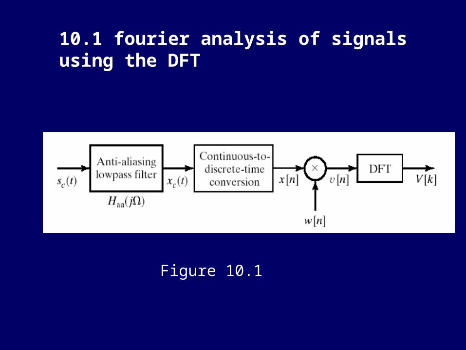
Figure 10.1
10.1 fourier analysis of signals using the DFT
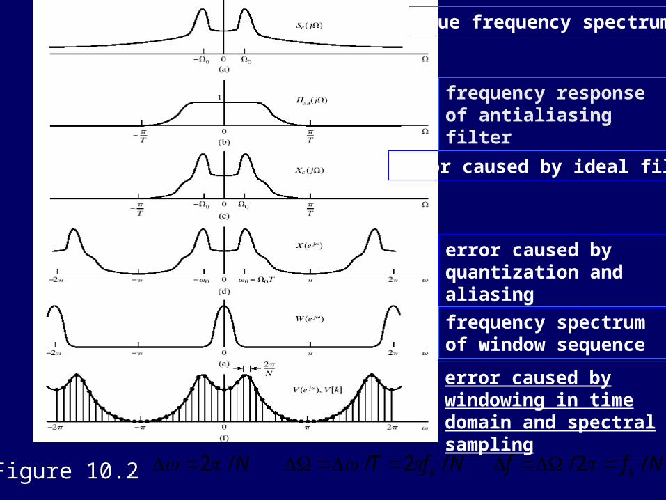
Figure 10.2
true frequency spectrum
error caused by ideal filter
error caused by quantization and aliasing
error caused by windowing in time domain and spectral sampling
frequency response of antialiasing filter
frequency spectrum of window sequence
NffNfTN ss /2/ /2/ /2
10.2 DFT analysis of sinusoidal signals
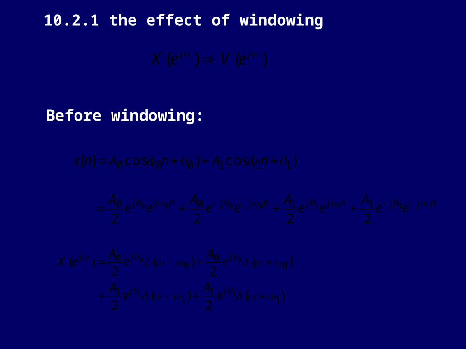
10.2.1 the effect of windowing
10.2.2 the effect of spectral sampling
)cos()cos(][ 111000 nAnAnx
10.2.1 the effect of windowing
)()( jj eVeX
)(2
)(2
)(2
)(2
)(
11
11
00
00
11
00
jj
jjj
eA
eA
eA
eA
eX
njjnjjnjjnjj eeA
eeA
eeA
eeA
11110000
22221100
Before windowing:
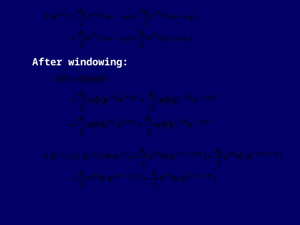
][][][ nwnxnv
)(2
)(2
)(2
)(2
)(*)()(
)(1)(1
)(0)(0
1111
0000
njjnjj
njjnjjjjj
eWeA
eWeA
eWeA
eWeA
eWeXeV
After windowing:
njjnjj
njjnjj
eenwA
eenwA
eenwA
eenwA
1111
0000
][2
][2
][2
][2
11
00
)(2
)(2
)(2
)(2
)(
11
11
00
00
11
00
jj
jjj
eA
eA
eA
eA
eX
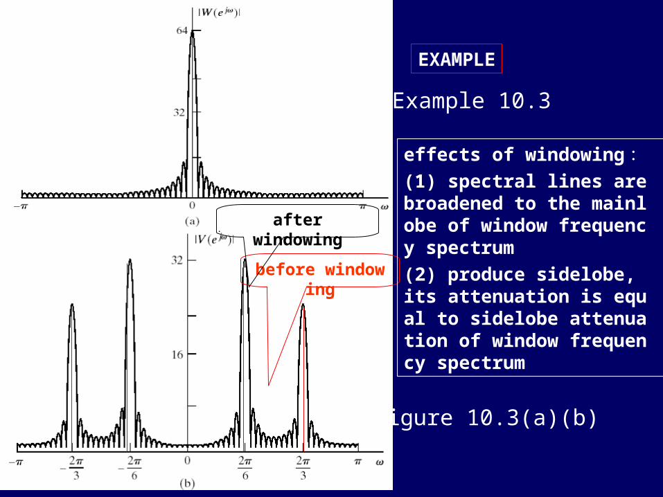
Figure 10.3(a)(b)
Example 10.3
EXAMPLE
|)(| jeX
before windowing
after windowing
effects of windowing:(1) spectral lines are broadened to the mainlobe of window frequency spectrum
(2) produce sidelobe, its attenuation is equal to sidelobe attenuation of window frequency spectrum
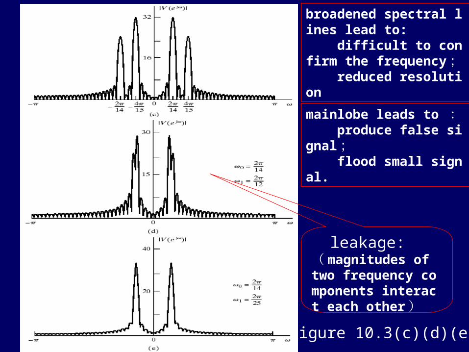
Figure 10.3(c)(d)(e)
broadened spectral lines lead to: difficult to confirm the frequency; reduced resolution
mainlobe leads to : produce false signal; flood small signal.
leakage:(magnitudes of two frequency components interact each other)
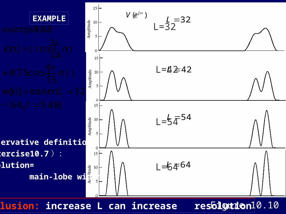
)48.5,64~
32(][
))15
4cos(75.0
)14
2(cos(][
:8.10
Lkaisernw
n
nnx
example
Conclusion: increase L can increase resolution Figure 10.10
EXAMPLE
42L
64L
32L
54L
L=32
L=42
L=54
L=64
conservative definition
( exercise10.7):resolution=
main-lobe width
)( jeV
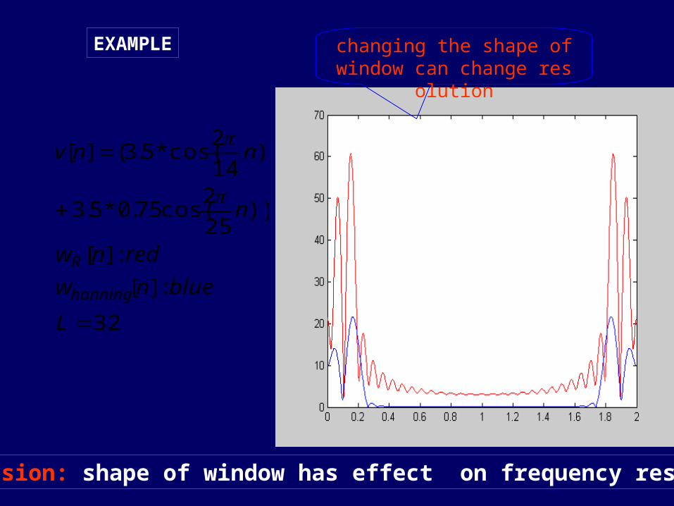
32
:][
:][
))25
2cos(75.0*5.3
)14
2cos(*5.3(][
L
bluenw
rednw
n
nnv
hanning
R
EXAMPLE changing the shape of window can change resolution
Conclusion: shape of window has effect on frequency resolution
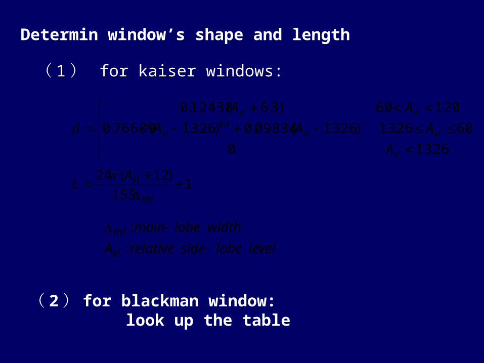
26.13
6026.13
12060
0
)26.13(09834.0)26.13(76609.0
)3.6(12438.04.0
sl
sl
sl
slsl
sl
A
A
A
AA
A
1155
)12(24
ml
slAL
Determin window’s shape and length
( 2) for blackman window: look up the table
( 1 ) for kaiser windows:
levellobesiderelativeA
widthlobemain
sl
ml
:
:
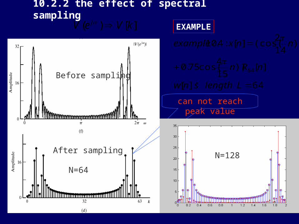
10.2.2 the effect of spectral sampling
][)( kVeV j
64]'[
][))15
4cos(75.0
)14
2(cos(][:4.10
64
Llengthsnw
nRn
nnxexample
EXAMPLE
Figure 10.5(a)(b)(f)
After sampling
Before sampling
can not reach peak value
N=64
N=128
N=64
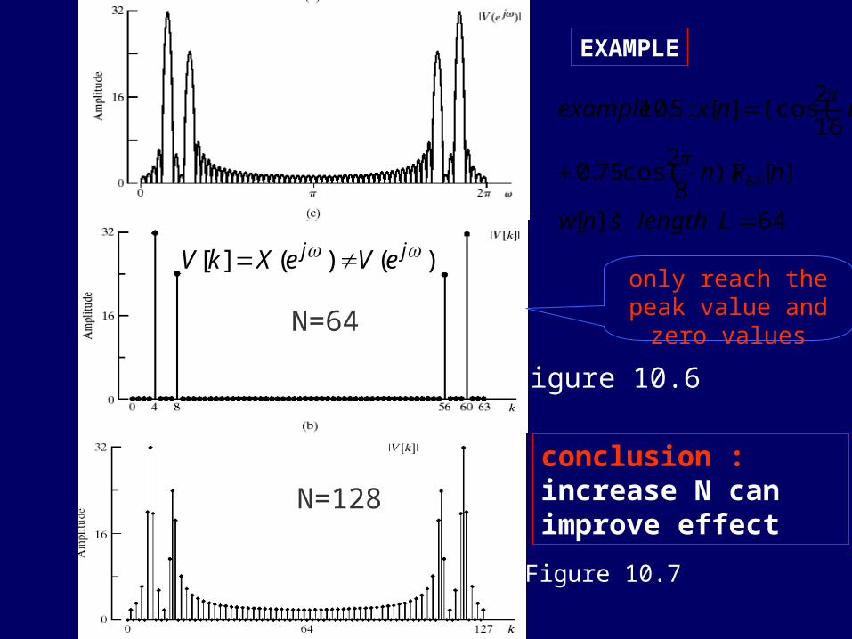
64]'[
][))8
2cos(75.0
)16
2(cos(][:5.10
64
Llengthsnw
nRn
nnxexample
Figure 10.6
EXAMPLE
)()(][ jj eVeXkV only reach the peak
value and zero values
N=128
Figure 10.7
N=64
N=128
conclusion : increase N can improve effect
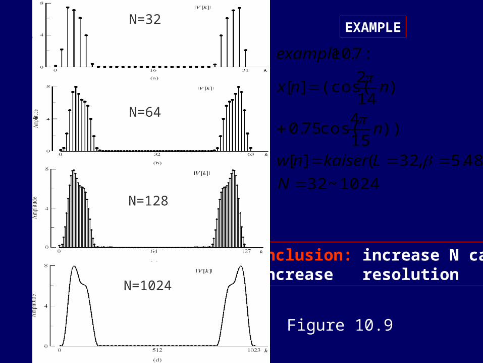
1024~32
)48.5,32(][
))15
4cos(75.0
)14
2(cos(][
:7.10
N
Lkaisernw
n
nnx
example
Figure 10.9
EXAMPLE
Conclusion: increase N can’t increase resolution
N=32
N=64
N=128
N=1024
N=32
N=64
N=128
N=1024

EXAMPLE
.difference their compare and ly,respective DFT, points 128 do
1280|)(][
/1,128640
630|)(][
,64,5.2,2),2cos()2cos()(
2
1
1121
ntfnf
fTn
ntfnf
HzfHzfHzftftftf
nTt
snTt
s
analyze effects of window length to DFT using MATLAB
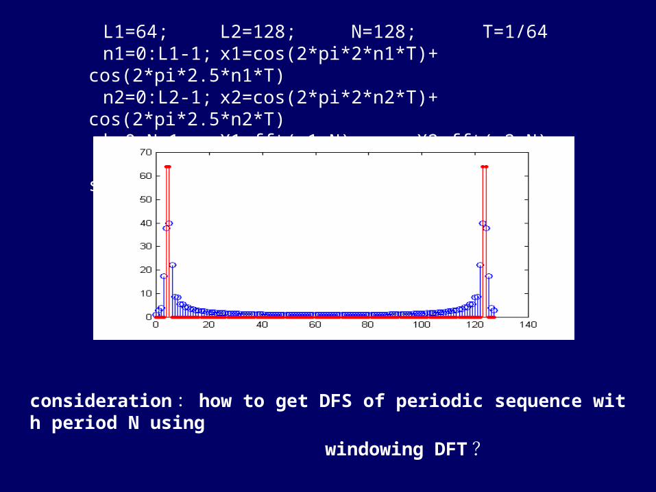
L1=64; L2=128; N=128; T=1/64n1=0:L1-1; x1=cos(2*pi*2*n1*T)+ cos(2*pi*2.5*n1*T)n2=0:L2-1; x2=cos(2*pi*2*n2*T)+ cos(2*pi*2.5*n2*T)k=0:N-1; X1=fft(x1,N); X2=fft(x2,N)stem(k,abs(X1)); hold on; stem(k,abs(X2),’r.’);
consideration: how to get DFS of periodic sequence with period N using
windowing DFT?
m
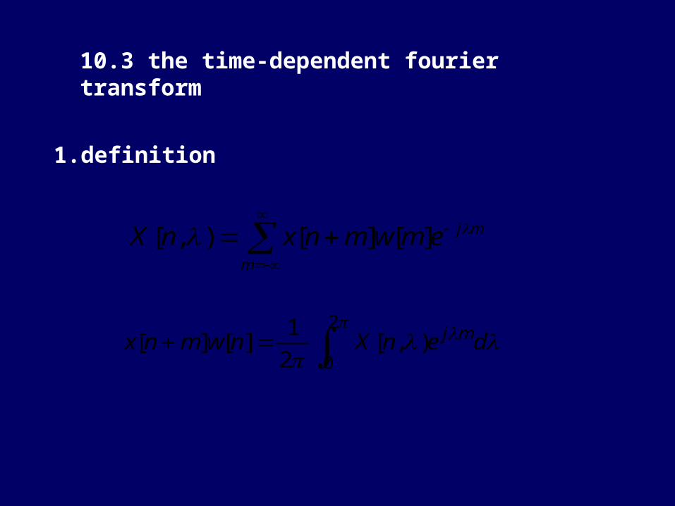
mjemwmnxnX ][][),[
10.3 the time-dependent fourier transform
1.definition
2
0),[
2
1][][ denXnwmnx mj
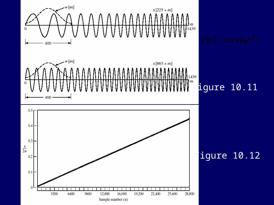
Figure 10.11
Figure 10.12
)cos(][ 20nnx
summary
10.1 fourier analysis of signals using the DFT
10.2 DFT analysis of sinusoidal signals
conclusion: effects of windowing and spectral sampling
10.3 the time-dependent fourier transform
apply the conclusion in 10.2 in analysis of general signals

requirements:effects of windowing and sampling to DFT line;
concept of frequency resolution, relationship among the shape and length of window , and the points of DFT;
DFT analysis of sinusoidal signals .
exercises and experiment
10.21 10.31(a)-(c)
experiment 31
34 and 35( draw them together)36
37( B)39( A)