10703DeepReinforcementLearningandControl

RussSalakhutdinovMachine Learning Department

rsalakhu@cs.cmu.edu

Exploration and Exploitation

Used Materials •  Disclaimer: Much of the material and slides for this lecture were borrowed from Rich Sutton’s class and David Silver’s class on Reinforcement Learning.

Exploration vs. Exploitation Dilemma

‣  Online decision-making involves a fundamental choice: -  Exploitation: Make the best decision given current information -  Exploration: Gather more information

‣  The best long-term strategy may involve short-term sacrifices

‣  Gather enough information to make the best overall decisions

Exploration vs. Exploitation Dilemma

‣  Restaurant Selection -  Exploitation: Go to your favorite restaurant -  Exploration: Try a new restaurant

‣  Oil Drilling -  Exploitation: Drill at the best known location -  Exploration: Drill at a new location

‣  Game Playing -  Exploitation: Play the move you believe is best -  Exploration: Play an experimental move

Exploration vs. Exploitation Dilemma

‣  Naive Exploration -  Add noise to greedy policy (e.g. ε-greedy)

‣  Optimistic Initialization -  Assume the best until proven otherwise

‣  Optimism in the Face of Uncertainty -  Prefer actions with uncertain values

‣  Probability Matching -  Select actions according to probability they are best

‣  Information State Search -  Look-ahead search incorporating value of information

The Multi-Armed Bandit

‣  A multi-armed bandit is a tuple ⟨A, R⟩

‣  A is a known set of k actions (or “arms”)

‣  is an unknown probability distribution over rewards

‣  At each step t the agent selects an action

‣  The environment generates a reward

‣  The goal is to maximize cumulative reward

Regret ‣  The action-value is the mean reward for action a,

‣  The optimal value V∗ is

‣  Maximize cumulative reward = minimize total regret

‣  The regret is the opportunity loss for one step

‣  The total regret is the total opportunity loss

‣  The gap ∆a is the difference in value between action a and optimal action a∗:

Counting Regret ‣  The count Nt(a): the number of times that action a has been selected

prior to time t

‣  A good algorithm ensures small counts for large gaps ‣  Problem: gaps are not known!

‣  Regret is a function of gaps and the counts

Counting Regret

‣  If an algorithm forever explores it will have linear total regret ‣  If an algorithm never explores it will have linear total regret ‣  Is it possible to achieve sub-linear total regret?

Greedy Algorithm

‣  We consider algorithms that estimate:

‣  Estimate the value of each action by Monte-Carlo evaluation:

‣  Greedy can lock onto a suboptimal action forever

‣  ⇒ Greedy has linear total regret

‣  The greedy algorithm selects action with highest value

Sample average

‣  The ε-greedy algorithm continues to explore forever

-  With probability 1 − ε select

-  With probability ε select a random action

ε-Greedy Algorithm

‣  ⇒ ε-greedy has linear total regret

‣  Constant ε ensures minimum regret

ε-Greedy Algorithm

2.3. INCREMENTAL IMPLEMENTATION 31

As you might suspect, this is not really necessary. It is easy to devise incrementalformulas for updating averages with small, constant computation required to processeach new reward. Given Qn and the nth reward, Rn, the new average of all n rewardscan be computed by

Qn+1 =1

n

nX

i=1

Ri

=1

n

Rn +

n�1X

i=1

Ri

!

=1

n

Rn + (n� 1)

1

n� 1

n�1X

i=1

Ri

!

=1

n

⇣Rn + (n� 1)Qn

⌘

=1

n

⇣Rn + nQn �Qn

⌘

= Qn +1

n

hRn �Qn

i, (2.3)

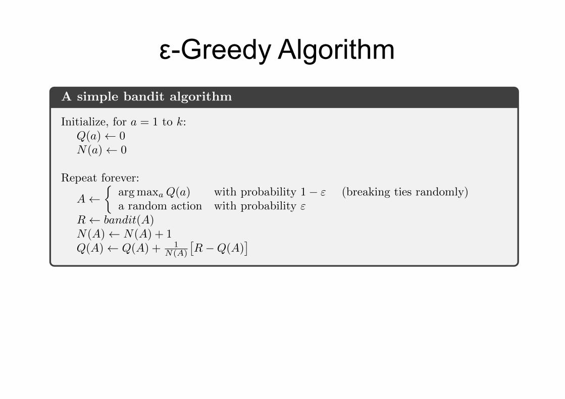
which holds even for n = 1, obtaining Q2 = R1 for arbitrary Q1. This implemen-tation requires memory only for Qn and n, and only the small computation (2.3)for each new reward. Pseudocode for a complete bandit algorithm using incremen-tally computed sample averages and "-greedy action selection is shown below. Thefunction bandit(a) is assumed to take an action and return a corresponding reward.

A simple bandit algorithm

Initialize, for a = 1 to k:Q(a) 0N(a) 0

Repeat forever:

A ⇢

arg maxa Q(a) with probability 1� " (breaking ties randomly)a random action with probability "

R bandit(A)N(A) N(A) + 1Q(A) Q(A) + 1

N(A)

⇥R�Q(A)

⇤

The update rule (2.3) is of a form that occurs frequently throughout this book.The general form is

NewEstimate OldEstimate + StepSizehTarget�OldEstimate

i. (2.4)

The expression⇥Target�OldEstimate

⇤is an error in the estimate. It is reduced by

taking a step toward the “Target.” The target is presumed to indicate a desirabledirection in which to move, though it may be noisy. In the case above, for example,the target is the nth reward.

Optimistic Initialization

‣  Encourages systematic exploration early on

‣  But can still lock onto suboptimal action

‣  Simple and practical idea: initialize Q(a) to high value

‣  Update action value by incremental Monte-Carlo evaluation

‣  Starting with N(a) > 0

Decaying εt-Greedy Algorithm

‣  Decaying εt-greedy has logarithmic asymptotic total regret

‣  Unfortunately, schedule requires advance knowledge of gaps

‣  Goal: find an algorithm with sub-linear regret for any multi-armed bandit (without knowledge of R)

‣  Pick a decay schedule for ε1, ε2, ...

‣  Consider the following schedule Smallest non-zero gap

Optimism in the Face of Uncertainty

‣  Which action should we pick? ‣  The more uncertain we are about an action-value ‣  The more important it is to explore that action ‣  It could turn out to be the best action

Optimism in the Face of Uncertainty

‣  After picking blue action ‣  We are less uncertain about the value ‣  And more likely to pick another action ‣  Until we home in on best action

Upper Confidence Bounds ‣  Estimate an upper confidence Ut(a) for each action value

‣  Such that with high probability

‣  This depends on the number of times N(a) has been selected -  Small Nt(a) ⇒ large Ut(a) (estimated value is uncertain) -  Large Nt(a) ⇒ small Ut(a) (estimated value is accurate)

Estimated mean Estimated Upper Confidence

‣  Select action maximizing Upper Confidence Bound (UCB)

Hoeffding’s Inequality

‣  We will apply Hoeffding’s Inequality to rewards of the bandit conditioned on selecting action a

Calculating Upper Confidence Bounds

‣  Pick a probability p that true value exceeds UCB

‣  Now solve for Ut(a)

‣  Reduce p as we observe more rewards, e.g. p = t−c, c=4 (note: c is a hyper-parameter that trades-off explore/exploit)

‣  Ensures we select optimal action as t → ∞

UCB1 Algorithm

‣  This leads to the UCB1 algorithm

Bayesian Bandits

‣  Bayesian bandits exploit prior knowledge of rewards,

‣  So far we have made no assumptions about the reward distribution R -  Except bounds on rewards

‣  Use posterior to guide exploration -  Upper confidence bounds (Bayesian UCB) -  Probability matching (Thompson sampling)

‣  Better performance if prior knowledge is accurate

‣  They compute posterior distribution of rewards -  where the history is:

Bayesian UCB Example

‣  Compute Gaussian posterior over µa and σa2 (by Bayes law)

‣  Assume reward distribution is Gaussian,

‣  Pick action that maximizes standard deviation of Q(a)

Probability Matching

‣  Can be difficult to compute analytically.

‣  Probability matching selects action a according to probability that a is the optimal action

‣  Probability matching is optimistic in the face of uncertainty -  Uncertain actions have higher probability of being max

Thompson Sampling

‣  Thompson sampling implements probability matching

‣  Use Bayes law to compute posterior distribution:

‣  Sample a reward distribution R from posterior

‣  Compute action-value function:

‣  Select action maximizing value on sample:

Value of Information

‣  Exploration is useful because it gains information

‣  Information gain is higher in uncertain situations

‣  Therefore it makes sense to explore uncertain situations more

‣  If we know value of information, we can trade-off exploration and exploitation optimally

‣  Can we quantify the value of information? -  How much reward a decision-maker would be prepared to pay in

order to have that information, prior to making a decision -  Long-term reward after getting information vs. immediate reward

Contextual Bandits

‣  A contextual bandit is a tuple ⟨A, S , R⟩

‣  A is a known set of k actions (or “arms”)

‣  is an unknown distribution over states (or “contexts”)

‣  is an unknown probability distribution over rewards

‣  The goal is to maximize cumulative reward

‣  At each time t -  Environment generates state -  Agent selects action -  Environment generates reward

Exploration/Exploitation for MDPs

‣  The same principles for exploration/exploitation apply to MDPs -  Naive Exploration -  Optimistic Initialization -  Optimism in the Face of Uncertainty -  Probability Matching -  Information State Search

Optimistic Initialization: Model-Free RL

‣  Initialize action-value function Q(s,a) to

‣  Run favorite model-free RL algorithm -  Monte-Carlo control -  Sarsa -  Q-learning -  …

‣  Encourages systematic exploration of states and actions

Optimistic Initialization: Model-Based RL

‣  Construct an optimistic model of the MDP

‣  Initialize transitions to go to heaven -  (i.e. transition to terminal state with rmax reward)

‣  Encourages systematic exploration of states and actions

‣  e.g. RMax algorithm (Brafman and Tennenholtz)

‣  Solve optimistic MDP by favourite planning algorithm -  policy iteration -  value iteration -  tree search -  …

Upper Confidence Bounds: Model-Free RL

‣  Maximize UCB on action-value function Qπ(s,a)

‣  Remember UCB1 Algorithm:

How do we estimate the counts in continuous spaces?

Bayesian Model-Based RL

‣  Maintain posterior distribution over MDP models

‣  Estimate both transitions and rewards, -  where the history is:

‣  Use posterior to guide exploration -  Upper confidence bounds (Bayesian UCB) -  Probability matching (Thompson sampling)

Thompson Sampling: Model-Based RL

‣  Thompson sampling implements probability matching

‣  Use Bayes law to compute posterior distribution:

‣  Sample from posterior an MDP P, R

‣  Solve MDP using favorite planning algorithm to get

‣  Select optimal action for sampled MDP,

Information State Search in MDPs

‣  MDPs can be augmented to include information state

‣  Now the augmented state is ⟨s,s~⟩ -  where s is original state within MDP -  and s~ is a statistic of the history (accumulated information)

‣  Each action a causes a transition -  to a new state s′ with probability -  to a new information state s~′

‣  Defines MDP in augmented information state space

Conclusion

‣  Have covered several principles for exploration/exploitation -  Naive methods such as ε-greedy -  Optimistic initialization -  Upper confidence bounds -  Probability matching -  Information state search

‣  These principles were developed in bandit setting

‣  But same principles also apply to MDP setting