10th international probabilistic workshop
TRANSCRIPT

10th
International Probabilistic Workshop
15 / 16 November 2012 in Stuttgart
Edited by
Christian Moormann
Maximilian Huber
Dirk Proske
Institut für Geotechnik der Universität Stuttgart
2012

Mitteilung 67
des Instituts für Geotechnik
Universität Stuttgart, Germany, 2012
Herausgeber:
Univ.-Prof. Dr.-Ing.habil. Christian Moormann
Institut für Geotechnik
Universität Stuttgart
Pfaffenwaldring 35
D - 70569 Stuttgart
Alle Rechte, insbesondere die der Übersetzung in andere Sprachen, vorbehalten.
Kein Teil dieses Buches darf ohne schriftliche Genehmigung des Herausgebers
in irgendeiner Form - durch Fotokopie, Mikrofilm oder irgendein anderes Ver-
fahren – reproduziert oder in eine von Maschinen, insbesondere von Datenver-
arbeitungsmaschinen, verwendbare Sprache übertragen oder übersetzt werde.
Druck: DCC Siegmar Kästl e.K, Stuttgart, Deutschland, 2012
ISBN 978-3-921837-67-2
Moormann, Huber & Proske: Proceedings of the 10th International Probabilistic Workshop, Stuttgart 2012
i
Preface
Safety, reliability and risk are key issues in a world with continuously increas-
ing complexity. Road and railway accidents, tunnel fires or natural hazards
like hurricanes, floods or earthquakes show the vulnerability of our technical
facilities and the natural and social environment. Therefore the consideration
of safety and risk is without doubt a very important issue during the design of
technical facilities, such as civil engineering structures and infrastructure
works. Questions about the analysis and treatment of safety and risk arise, as
well as questions about optimal safety levels or questions about acceptable
values.
In 2012 we celebrate 10 years of the symposium "International Probabilistic
Workshop". This series of probabilistic workshops on safety and risk in civil
engineering were organized starting 2003/2004 in Dresden, followed 2005 in
Vienna, 2006 in Berlin, 2007 in Ghent, 2008 in Darmstadt, 2009 in Delft,
2010 in Szczecin and 2011 in Braunschweig. During all this symposiums
more than 200 presentations were given and thousands of pages were written
for the conference proceedings. The covers of the proceedings of these former
symposiums can be seen on the next page. Besides the proceedings, special
issues of the journals "Structure and Infrastructure Engineering", "Beton- und
Stahlbetonbau" and "Georisk" based on expanded papers from symposiums
were published.
This series is continued with the 10th
Probabilistic Workshop at University of
Stuttgart, which is organised jointly by the Institute of Geotechnical Engineer-
ing of the University of Stuttgart and the Institute of Natural Hazards, Univer-
sity of Natural Resources and Applied Life Sciences-Vienna.
Four internationally renowned keynote speakers will lecture on risk, reliabil-
ity and probability methods in mechanical engineering, geotechnical engi-
neering, financial engineering and clinical economics. This year the
conference programme includes 21 contributions from prestigious authors
coming form all over the world, which have been reviewed by the scientific
committee in order to guarantee the quality of the work.
Finally, the organizers are grateful to all those who have helped and contrib-
uted to the organisations of this event. The largest part of the credit for theses

Preface
ii
proceedings goes to the authors, speakers and the reviewers, not only for this
conference, but for all conferences in this series.
We look forward to the interesting presentations, animated discussions and
gracious meetings at our conference. Furthermore the editors hope that this set
of papers can be a useful reference for many readers.
Christian Moormann, Maximilian Huber & Dirk Proske
Editors

Moormann, Huber & Proske: Proceedings of the 10th International Probabilistic Workshop, Stuttgart 2012
iii

Preface
iv
Moormann, Huber & Proske: Proceedings of the 10th International Probabilistic Workshop, Stuttgart 2012
v
Table of contents
I. Elishakoff 1
Recent developements in applied mechanics with uncertainties
W. Betz, I. Papioannou & D. Straub 3
Quasi meshless discretization of random fields based on the
Karhunen-Loeve expansion
P. Criel, R. Caspeele & L. Taerwe 19
Using Bayesian response surface updating for estimating the covari-
ance function of random fields based on measurements
H. Keitel 33
Assessing the prediction quality of coupled partial models taking into
account coupling quality
T. Poutanen 47
Dependent load combination
D. Charmpis 61
Reliability based design optimization of damage- tolerant elastoplastic
frames
T. Vallee, T. Tannert & C.Grunwald 75
Seemingly contradictory: influence of stress-reduction-methods on the
strength of bonded joints composed of brittle adherends
F. Porzsolt 91
Risk Management in Health Care - Lessons learned from Clinical
Economics
D. Casali, A. Colios & N. Antoniadis 111
Systematic uncertainty quantification of pipe flow systems
S. Kessler & C. Gehlen 127
Probability of detection of potential mapping

Table of contents
vi
C. McLeod, J. Wium & J. Retief 141
Reliability model for cracking in South African reinforced concrete
water retaining structures
R. Riebeek 157
Challenges in modelling in banking: behaviour and usability"
D. Bach & P. van Gelder 165
Resistance factor calibration of drilled shafts for bridge foundations
V. Boros & B. Novák 189
Reliability and risk analysis of concrete bridges for hazard scenarios
M. Akramin, A. Ariffin, M. Kikuchi, S. Abdullah, N. Nikabdullah &
M. Shaari
203
Probabilistic analysis based on s-FEM of surface crack growth
M. Hicks & J. Nuttdall 215
Influence of soil heterogeneity on geotechnical performance and un-
certainty
B. Jung, H. Stutz, G. Morgentha & F. Wuttke 229
Uncertainty Analysis of deep foundation models in bridge engineering
A. Nasekhian, H. F. Schweiger & T. Marcher 243
Random Set against Point Estimate Method – A case study in tunnelling
M. Sättele, M. Brünld & D. Straub 257
Warning and alarm systems for natural hazards - a classification and
generic system break-down
V. Bayer 271
Random field methods in robustness analysis
H. Motra, A. Dimmig-Osburg & J. Hildebrand 285
Probabilistic assessment of concrete creep models under repeated
loading with correlated and uncorrelated input variables

Moormann, Huber & Proske: Proceedings of the 10th International Probabilistic Workshop, Stuttgart 2012
vii
I. Skrzypczak 303
Fuzzy and statistical conformity criteria for compressive strength ac-
cording to the EN 206-1 code
R. Van Coile, R. Caspeele & L. Taerwe 313
Quantifying the structural safety of concrete slabs subjected to the
ISO 834 standard fire curve using full-probabilistic FEM
N. A. N. Mohamed, S.S. K. Singh & M. S. Md Noorani 331
Reliability of a crankshaft by using Markov Chain Model with a prob-
abilistic approach
M. Holicky & M. Sykora 345
Probabilistic assessment of existing structures
T. Zimmermann, K. Haider & A. Strauss 357
Stochastic material properties for different concrete types:
An experimental investigation
A. Krawtschuk, T. Zimmermann, K. Haider, A.Strauss & O.Zeman 367
Development of a finite element model for masonry arch bridges in-
corporating stochastic material parameters

Table of contents
viii
Moormann Huber & Proske: Proceedings of the 10th International Probabilistic Workshop, Stuttgart 2012
1
Recent Developments in Applied Mechanics
with Uncertainties
Isaac Elishakoff
Department of Ocean and Mechanical Engineering
Florida Atlantic University
Boca Raton, FL 33431-0991, U.S.A.
It has been recognized during past decades that deterministic mechanics as
such cannot answer all problems that arise in engineering. For example, the
safety factor that is being utilized in engineering design cannot possibly be
justified within deterministic mechanics. Thus, the uncertainty analysis is in-
troduced in deterministic analysis ‘via the back door.’ The realistic analysis
and design of structures demands the introduction of uncertainty analyses. To
accomplish this goal, until very recently the only methodology used was the
probabilistic analysis. It is interesting to note that the first attempt to do so,
appears to have been a dissertation by Max Mayer titled Die Sicherheit der
Bauwerke und ihre Berechnung nach Grenzkraeften astatt nach zulaessigen
Spannungen, published in 1926 by Springer. In this spirit the lecture reviews
first the safety factor idea and then the most common method that is applied
in stochastic analysis of nonlinear structures, namely the stochastic lineariza-
tion technique.
Then the lecture deals with alternatives to probability analysis: interval and
ellipsoidal analyses and shows which one should be used in which circum-
stances .In these analyses no probability or fuzzy measures are needed to be
known. These analyses depend on scarce knowledge—that is often the case-
for involved uncertain variables. Instead the bounds--as either intervals or el-
lipsoids--are incorporated into the analysis. The notion of combined optimiza-
tion and anti-optimization will be discussed. At the last part the lecture
reviews the notion of the fuzzy safety factor.
Recent Developments in Applied Mechanics with Uncertainties
2
Many researchers prefer to use one of these techniques exclusively and main-
tain that only one of these methods is useful. In fact it appears that there is, as
it were, a Babel Tower erected between different methodologies of uncertain-
ty analyses. As pragmatic creatures engineers appear to be in need to know
each of these techniques and use them in different circumstances depending
on the character and the amount of available data.
References
Elishakoff, I., Probabilistic Theory of Structures, Dover, Mineola, NY, 1999.
Elishakoff, I., Safety Factors and Reliability: Friends or Foes, Kluwer, Dor-
drecht, 2004.
Elishakoff, I. and Ohsaki M., Optimization and Anti-Optimization of Struc-
tures under Uncertainty, Imperial College Press, London,
2010.

Moormann, Huber & Proske: Proceedings of the 10th International Probabilistic Workshop, Stuttgart 2012
3
A finite cell approach for discretization of
random fields
Wolfgang Betz1, Iason Papaioannou, Daniel Straub
Engineering Risk Analysis Group, Faculty of Civil Engineering and Geodesy,
Technische Universität München, Germany
Abstract: A new method for discretization of Gaussian random fields with on-
ly a small number of random variables in the representation is introduced. The
method is based on the Karhunen-Loève (KL) expansion, which is optimal
among series expansion methods with respect to the global mean square trun-
cation error. The resulting integral eigenvalue problem in the KL-expansion is
discretized using a finite cell (FC) approach; i.e. the domain of computation is
extended beyond the physical domain up to the boundaries of an embedding
domain with a primitive geometrical shape. Higher order polynomials are used
as FC shape functions. The approach is useful for random fields defined on
domains with complex geometries since it shifts the problem from the mesh
generation to the integration of discontinuous functions defined over a ficti-
tious domain. A suitable approach for numerical integration is described. The
presented method is compared to the Expansion Optimal Linear Estimation
(EOLE) method and to the finite element discretization of the KL-expansion
with respect to the mean error variance and in terms of computational costs. On
the one hand, the proposed approach shows an exponential rate of convergence
in terms of the dimension of the matrix eigenvalue problem to solve for a fixed
number of random variables. On the other hand, obtaining a solution for the
random field approximation takes considerably longer than with the EOLE
method. However, the generation of a realization of the random field represen-
tation with the finite cell approach is computationally more efficient than with
EOLE.
1 Introduction
A stochastic analysis of structures in civil engineering often requires the mod-
eling of input parameters that vary randomly in space (e.g. load distributions
or material parameters). This type of uncertainty is modeled by means of ran-
1 With the support of the Technische Universität München - Institute for Advanced Study, funded by the
German Excellence Initiative.
Betz; Papaioannou; Straub: A finite cell approach for discretization of random fields
4
dom fields. A random field represents a random quantity at each point of a
continuous domain, and, thus, consists of an infinite number of random varia-
bles. For computational purposes, the random field has to be expressed using
a finite number of random variables. This step is referred to as random field
discretization.
The efficiency of a random field discretization method depends on its ability
to approximate the original random field accurately with a minimum number
of random variables. Accuracy is to be defined with respect to a certain error
measure such as the global mean square truncation error. It is advantageous to
keep the number of random variables in the representation of the random field
small, since it can have a considerable influence on the computational costs of
a subsequent stochastic analysis. An example is finite element reliability
analysis [2] where, for instance, a first-order reliability method (FORM) is
employed to obtain an estimate of the failure probability of the investigated
system. Another example is the spectral stochastic finite element method [4].
For this method, the size of the problem to solve is a function involving facto-
rials of the input random variables and, thus, the problem size increases dras-
tically with increasing number of random variables. An overview of random
field discretization methods is given in [9].
The Karhunen-Loève (KL) expansion of random fields is optimal in the glob-
al mean square truncation error with respect to the number of random varia-
bles in the representation [5]. However, its analytical solution is available
only for primitive geometries and for a few selected autocovariance functions.
For complex-shaped geometries, a finite element based approach can be cho-
sen to approximate the solution of the KL expansion. However, this requires a
spatial decomposition of the domain.
The requirements to a good random field mesh are not the same as the re-
quirements to a good mesh of the corresponding mechanical system (see [9]).
Consequently, two different meshes might be necessary. However, working
with different meshes is a handicap in writing efficient algorithms for post-
processing the random field (e.g. evaluating the realization of the field at eve-
ry finite element Gauss-point). A possible remedy is to use the elements in the
FE mesh as a basis for the random field mesh, and to adapt the mesh by either
refining individual elements or by coalescing different elements. This ap-
proach becomes impractical for two- or three-dimensional problems if the
physical domain is of complex geometrical shape. This includes domains with
curved boundaries, domains with holes, and porous media. Therefore, mesh-
less approaches appear to be favorable on complex shaped domains.
Moormann, Huber & Proske: Proceedings of the 10th International Probabilistic Workshop, Stuttgart 2012
5
The Expansion Optimal Linear Estimation (EOLE) method [6] does not re-
quire a mesh; the domain of the field is approximated by a number of points.
Consequently, the shape of the physical domain is of minor importance, since
the selection of points can be easily performed on a fictitious domain contain-
ing the actual physical domain, where all points outside of the physical do-
main are neglected. Another meshless approach [7] is to embed the physical
domain in a larger domain of primitive geometrical shape. The KL expansion
is then solved for the primitive domain, either analytically or numerically.
However, the optimality of the KL expansion with respect to the mean square
truncation error is lost in this approach since the expansion is solved on a do-
main that is larger than the actual physical domain.
The finite cell (FC) method [8] is a fictitious domain approach, developed as
an extension of the finite element method. Following this approach, the phys-
ical domain is embedded in elements of primitive geometrical shape. Higher
order shape functions are of crucial importance for the applicability of the
method because they yield a fast rate of convergence [8]. The finite cell
method shifts the problem of complex geometries from the mesh generation
to the integration.
In this work, a finite cell like approach is utilized to discretize the spatial do-
main of the random field and, thus, to approximate the solution of the
Karhunen-Loève expansion numerically. The proposed method inherits the
efficiency of the KL expansion if the error in the numerical integration is neg-
ligible and if the eigenmodes of the KL expansion can be approximated well
by the chosen shape functions. The presented method is compared to the
EOLE method and to the finite element discretization of the KL-expansion.
The proposed approach shows an exponential rate of convergence with re-
spect to the size of the matrix eigenvalue problem to solve. On the other hand,
obtaining a solution for the random field approximation takes considerably
longer than with the EOLE method. However, the generation of a realization
of the random field representation with the finite cell approach is more effi-
cient in terms of computational cost than with EOLE.
2 Discretization of random fields
A continuous random field ),( xH may be loosely defined as a random func-
tion that describes a random quantity at each point x of a continuous do-
main dR , 0Nd . is a coordinate in the sample space , and
),,( PF is a complete probability space. If the random quantity attached to
each point x is a random variable, the random field is said to be univariate or

Betz; Papaioannou; Straub: A finite cell approach for discretization of random fields
6
real-valued. If the random quantity is a random vector, the field is called mul-
tivariate. The dimension d of a random field is the dimension of its topologi-
cal space . One usually distinguishes between a one- and a
multidimensional random field, the former one is also referred to as random
process. The field is said to be Gaussian if the distribution of
)),(,),,(( 1 nHH xx is jointly Gaussian for any ),,( 1 nxx and any
0Nn . It is completely defined by its mean function Rx :)( and auto-
covariance function Rxx :)',(Cov . In the following, we will restrict
ourselves to continuous univariate multidimensional Gaussian random fields.
The approximation )(ˆ H of a continuous random field )(H by a finite set of
random variables Mii ,,1),( is referred to as random field discretiza-
tion.
2.1 Error measures
Different error measures are available to quantify the error resulting from the
discretization of a random field. For a given outcome , the truncation error
)(H is defined at position x as the difference between the random field and
its approximation:
).,(ˆ),(),( xxx HHH (1)
In the context of this work, we will assume that the mean function of the ap-
proximated random field can be modeled precisely, i.e. xx 0),(E H .
In general, the truncation error can only be evaluated if the exact representa-
tion of the random field is known explicitly. This is usually not the case. In
the following, an error estimator is introduced which circumvents this prob-
lem. )(x is known as the error variance and has been commonly used in the
literature; it is defined as:
,
)(
),(ˆ),(Var
),(Var
),(ˆ),(Var)(
2 x
xx
x
xxx
HH
H
HH
(2)
where )(x is the standard deviation function of the random field ),( xH .
Pointwise measures are of little use when making a quantitative assessment of
the quality of the overall random field approximation. Therefore, the follow-
ing global error norm , known as the mean error variance, is used here:
Moormann, Huber & Proske: Proceedings of the 10th International Probabilistic Workshop, Stuttgart 2012
7
xx d)(
(3)
where xd . Besides the mean error variance, other global error measures
haven been used in the literature. For example, in [6] the supremum norm of
the error variance was used to compare different random field discretization
methods. It has been noted in [10] that different global error measures might
favor different discretization methods. In this work, we will only investigate
convergence with respect to the mean error variance.
2.2 Karhunen-Loève expansion
The KL-expansion is a series expansion method for the representation of a
random field. The expansion is based on the spectral decomposition of the
covariance function of the field. It states that a random field can be represent-
ed exactly by the following expansion:
1
)()(),(i
iiiH xxx (4)
where )(x is the mean function of the field, i are independent standard
normal random variables, and i , )(xi are the eigenvalues and eigenfunc-
tions of the covariance kernel obtained from solving the integral eigenvalue
problem:
)('d)',Cov()( xxxxx iii
(5)
The eigenfunctions are by definition orthonormal, i.e. ijji xxx d )( )( ,
where ij is the Kronecker delta.
2.2.1 Truncated Karhunen-Loève expansion
The truncated KL-expansion is obtained by arranging the eigenvalues and ei-
genfunctions in a descending series with respect to the magnitude of the ei-
genvalues, and truncating the ordered expansion after M terms. The truncated
KL-expansion does no longer represent the random field )(xH exactly, but
provides an approximation )(~
xH of the field. Hence, the truncated KL-
expansion is a random field discretization method. The discretized random
field is written as:
Betz; Papaioannou; Straub: A finite cell approach for discretization of random fields
8
M
i
iiiH1
)()(),(~
xxx (6)
An important property of the truncated KL-expansion is that the global mean
square error is minimized with respect to any other complete basis of )(2 L
[5].
2.2.2 Error variance
For the truncated KL-expansion, the error variance can be expressed as [9]:
)(
)(1)(
2
1
2
x
xx
M
i ii (7)
2.3 Finite element approximation of the KL-expansion
The KL-expansion involves solving the integral eigenvalue problem given in
equation 5. Equation 5 can be solved analytically only for a few covariance
functions and geometries (see [5]). Therefore, for general problems with arbi-
trary geometries and covariance functions, a numerical approach is necessary.
This involves a spatial discretization of the integral eigenvalue problem. Ob-
viously, this introduces yet another approximation to the representation of the
random field. The obtained eigenvalues i and eigenfunctions )(ˆ xi are,
therefore, approximations to the eigenvalues i and eigenfunctions )(xi of
the analytical solution of the KL-expansion. The approximation of the random
field can be expressed as:
M
i
iiiH1
)(ˆˆ)(),(ˆ xxx (8)
In the finite element approximation of the KL-expansion (in the following
referred to as FE-KL method), the eigenfunctions are approximated as:
N
n
in
i
ni Nd1
T )()()(ˆ dxNxx (9)
where N is the number of shape functions, )()( 2 LN n x are the global shape
functions forming a basis in a chosen sub-space of the set of all Lebesgue
square-integrable functions on , and Ri
nd are the coordinates of the ith
eigenfunction in the basis formed by all shape functions. )(TxN is a vector
function of x with elements )(xnN , and id is a vector containing the coeffi-
Moormann, Huber & Proske: Proceedings of the 10th International Probabilistic Workshop, Stuttgart 2012
9
cients i
nd . It is important to note that the eigenfunctions are by definition or-
thonormal and, therefore, the vectors id have to be scaled appropriately.
The approximation of the integral eigenvalue problem defined in equation 5
by means of equation 9 introduces an error term, denoted )(xi
N . The coeffi-
cients of the vectors id are selected such that the error term )(xi
N becomes
orthogonal to the space spanned by the shape functions. A solution to this
problem is given by the matrix eigenvalue problem:
iii MdBd (10)
The coefficients knB of the matrix B are defined as:
x x
xxxxxx d 'd )',Cov()'( )('
nkkn NNB (11)
The coefficients knM of the matrix M are defined as:
x
xxx d )( )( nkkn NNM (12)
The error variance of the FE-KL approach can be expressed as [1]:
)(
' )'(ˆ)',Cov()(ˆ2)(ˆˆ
1)(2
1
2
1
2
x
xxxxxxx
M
i ii
M
i ii d (13)
In case of a constant standard deviation within the domain of the field, the
mean error variance reduces to (compare [1]):
M
i
i
12
ˆ11
(14)
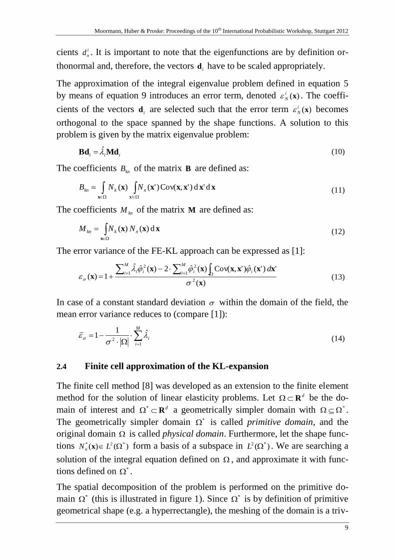
2.4 Finite cell approximation of the KL-expansion
The finite cell method [8] was developed as an extension to the finite element
method for the solution of linear elasticity problems. Let dR be the do-
main of interest and dR* a geometrically simpler domain with * .
The geometrically simpler domain * is called primitive domain, and the
original domain is called physical domain. Furthermore, let the shape func-
tions )()( *2* LNn x form a basis of a subspace in )( *2 L . We are searching a
solution of the integral equation defined on , and approximate it with func-
tions defined on * .
The spatial decomposition of the problem is performed on the primitive do-
main * (this is illustrated in figure 1). Since * is by definition of primitive
geometrical shape (e.g. a hyperrectangle), the meshing of the domain is a triv-
Betz; Papaioannou; Straub: A finite cell approach for discretization of random fields
10
ial task. However, the region * is not part of the physical domain. In
order to solve the original, i.e. physical, problem, the non-physical part of the
extended domain * must not influence the solution. For this reason, we in-
troduce the mapping 1,0: * as:
otherwise0
1)(
xx (15)
In order to solve the problem defined in equation 10 we have to assemble the
matrices M and B . The integral in equation 12 can be transformed to an inte-
gral over * as:
*
d )( )( )(x
xxxx nkkn NNM (16)
In a similar way, the integral in equation 11 can be written as:
* *
d 'd )',Cov()'( )'( )( )(
'x x
xxxxxxxx nkkn NNB (17)
In the finite cell approach, the shape functions are defined locally on the cells
e , see Figure 1. Higher order hierarchical shape functions based on the inte-
grated Legendre polynomials [11] are used, compare [8]. Note that the inte-
grals in equations 16 and 17 are smooth over the domain but not even
continuous over the domain * . Therefore, it is important to use appropriate
numerical integration schemes in order to keep the integration error small.
Figure 1. Notation for the finite cell approach.
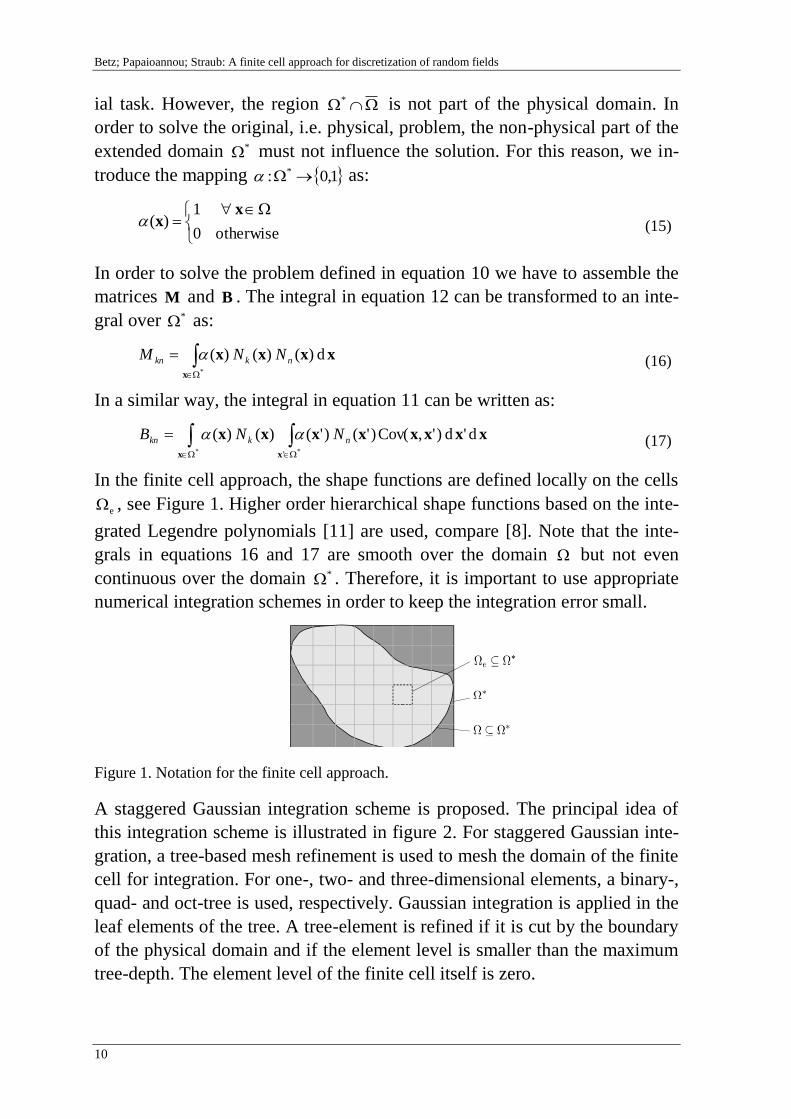
A staggered Gaussian integration scheme is proposed. The principal idea of
this integration scheme is illustrated in figure 2. For staggered Gaussian inte-
gration, a tree-based mesh refinement is used to mesh the domain of the finite
cell for integration. For one-, two- and three-dimensional elements, a binary-,
quad- and oct-tree is used, respectively. Gaussian integration is applied in the
leaf elements of the tree. A tree-element is refined if it is cut by the boundary
of the physical domain and if the element level is smaller than the maximum
tree-depth. The element level of the finite cell itself is zero.
Moormann, Huber & Proske: Proceedings of the 10th International Probabilistic Workshop, Stuttgart 2012
11
In the context of this work, the number of Gauss-points used on the respective
levels of the tree is decreased with an increasing level. This is contrary to the
approach presented in [8] and [3], where all sub-cells were integrated with a
full number of Gauss-points. However, in the cut-cells the function to inte-
grate is discontinuous and, therefore, cannot be approximated well using
polynomials. Moreover, the influence area of the individual Gauss-points is
not directly observable and not necessarily accumulated around the corre-
sponding point.
Figure 2. Staggered Gaussian integration: mesh for integration on a cut finite cell.
Assuming the integration error is small enough, )(x and can be comput-
ed according to equation 13 and 14, respectively.
2.5 EOLE method
The EOLE method [6] is a series expansion method that is based on an opti-
mal linear estimation using discrete points of the field and carries out a spec-
tral decomposition of the covariance matrix χχΣ corresponding to these
points. The coefficients of the covariance matrix are defined as
jiij ,CovχχΣ with },2,1{, Nji , where each i is a random variable
associated with a point ix .
The points ix are used to discretize the domain of the random field
pointwise. Consequently, the domain is represented approximately by a finite
number of points and no finite element mesh is required. The distribution of
the points ix has an influence on the random field approximation, especially
if the field is approximated by a minimal number of points.
The random field representation in case of the EOLE method writes:
M
i
i
i
T
iH
1
)()(),(ˆ
xΣΦxx
χX (18)
Betz; Papaioannou; Straub: A finite cell approach for discretization of random fields
12
where i and T
iΦ are the M largest eigenvalues and their corresponding ei-
genvectors of the covariance matrix χχΣ , the i are independent standard
normal random variables; )(xΣχX is a vector function whose coefficients are
defined as xxxΣχX ,Cov)( jj with Nj ,,2,1 . The EOLE method mini-
mizes the mean square error pointwise given values of the random field at the
set of points Nxxx ,,, 21 . For the EOLE method, the error variance can be
expressed as [6]:
M
i i
T
i
1
2
2
)(
)(
11)(
xΣΦ
xx
χX (19)
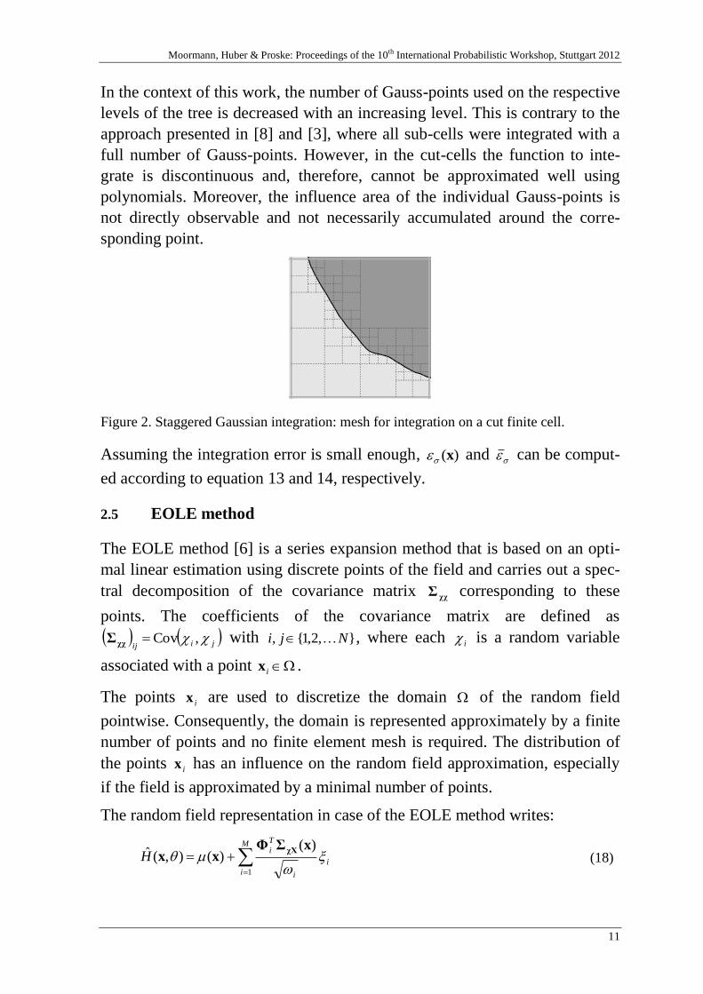
3 Numerical convergence study
The convergence behavior of the proposed finite cell approach with respect to
the mean error variance is investigated by means of a numerical example. The
random field is modeled for a squared domain with a circular hole in its cen-
ter. The length of a side of the square is four and the diameter of the circular
hole is two, as shown in figure 3. The Gaussian random field has a constant
mean value and standard deviation of 31030 and 3106 , respectively.
2
2
2
4
4
Figure 3. Domain used for the numerical convergence study.
Three different types of correlation coefficient functions are considered:
2
'exp', :A Type
A
xxxx (20)
B
'exp', :B Type
xxxx
(21)
Moormann, Huber & Proske: Proceedings of the 10th International Probabilistic Workshop, Stuttgart 2012
13
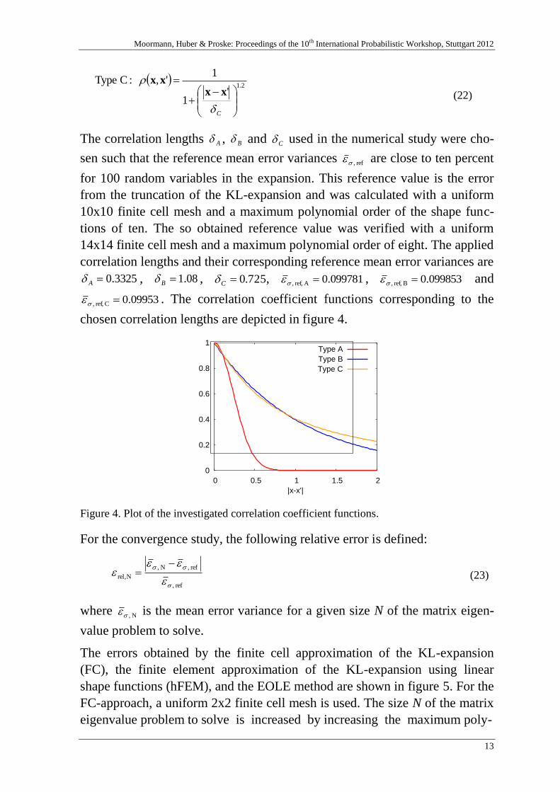
The correlation lengths A , B and C used in the numerical study were cho-
sen such that the reference mean error variances ref , are close to ten percent
for 100 random variables in the expansion. This reference value is the error
from the truncation of the KL-expansion and was calculated with a uniform
10x10 finite cell mesh and a maximum polynomial order of the shape func-
tions of ten. The so obtained reference value was verified with a uniform
14x14 finite cell mesh and a maximum polynomial order of eight. The applied
correlation lengths and their corresponding reference mean error variances are 3325.0A , 08.1B , 725.0C , 099781.0Aref, , , 099853.0Bref, , and
09953.0Cref, , . The correlation coefficient functions corresponding to the
chosen correlation lengths are depicted in figure 4.
0
0.2
0.4
0.6
0.8
1
0 0.5 1 1.5 2
co
rre
latio
n c
oe
ff.
fun
ctio
n
|x-x'|
Type A
Type B
Type C
Figure 4. Plot of the investigated correlation coefficient functions.
For the convergence study, the following relative error is defined:
ref ,
ref ,N ,
Nrel,
(23)
where N , is the mean error variance for a given size N of the matrix eigen-
value problem to solve.
The errors obtained by the finite cell approximation of the KL-expansion
(FC), the finite element approximation of the KL-expansion using linear
shape functions (hFEM), and the EOLE method are shown in figure 5. For the
FC-approach, a uniform 2x2 finite cell mesh is used. The size N of the matrix
eigenvalue problem to solve is increased by increasing the maximum poly-
2.1
'1
1', :C Type
C
xx
xx
(22)
Betz; Papaioannou; Straub: A finite cell approach for discretization of random fields
14
0.0001
0.001
0.01
0.1
1
100 1000 10000
rela
tive
err
or
N
FC
hFEM
EOLE
(a) convergence (Type A)
0.0001
0.001
0.01
0.1
1
100 1000 10000re
lative
err
or
N
FC
hFEM
EOLE
(b) convergence (Type B)
0.0001
0.001
0.01
0.1
1
100 1000 10000
rela
tive
err
or
N
FC
hFEM
EOLE
(c) convergence (Type C)
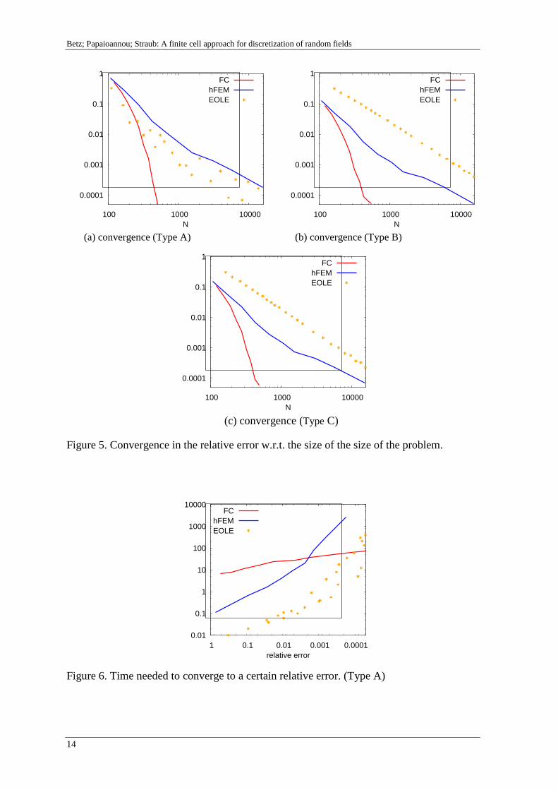
Figure 5. Convergence in the relative error w.r.t. the size of the size of the problem.
0.01
0.1
1
10
100
1000
10000
0.0001 0.001 0.01 0.1 1
tim
e [
s]
relative error
FC
hFEM
EOLE
Figure 6. Time needed to converge to a certain relative error. (Type A)
Moormann, Huber & Proske: Proceedings of the 10th International Probabilistic Workshop, Stuttgart 2012
15
nomial order of the shape functions. The maximum polynomial order in each
coordinate direction is the same. For the hFEM-approach, the actual physical
domain is meshed using four node quadrilateral elements. The problem size N
is increased by refining the mesh. In case of the EOLE-method, the problem
size N is equivalent to the total number of points used to discretize the field.
The points were distributed uniformly over the domain.
The plots (a), (b) and (c) in figure 5 show the relative error defined in equa-
tion 23 for an increasing size N of the matrix eigenvalue problem to solve.
The FC-approach shows an exponential rate of convergence for all three types
of correlation coefficient functions. The convergence rate of the hFEM-
method and the EOLE method is approximately linear in the log-log plots.
The EOLE-method converges faster than the hFEM-method for the correla-
tion coefficient function of type A. For the correlation coefficient functions of
type B and C, the hFEM-method converges faster than the EOLE-method.
Figure 6 shows the time needed for the methods to converge to a certain rela-
tive error for the correlation coefficient function of type A. To obtain a rea-
sonably well converged solution, the FC-approach needs considerably more
time than the hFEM-method and the EOLE-method. For this particular corre-
lation coefficient function, the EOLE-method solves the problem around one
order of magnitude faster than the hFEM-method.
In a next study, the time required to evaluate a realization of the random field
at a given position x is analyzed. This is of importance when the random field
is used as input to finite element reliability analysis, because a realization of
the field has to be evaluated at every finite element Gauss-point. In case of the
hFEM-approach, the time needed to evaluate a realization of the random field
at one position x does not depend on the mesh, because the number of shape
functions per element remains constant. Consequently, it remains constant
with increasing N. This time is denoted hFEMt in the following. On the other
hand, the time needed to obtain a realization depends in case of the FC-
approach on the maximum polynomial degree of the shape functions, and for
the EOLE-method on the number of points used to discretize the domain.
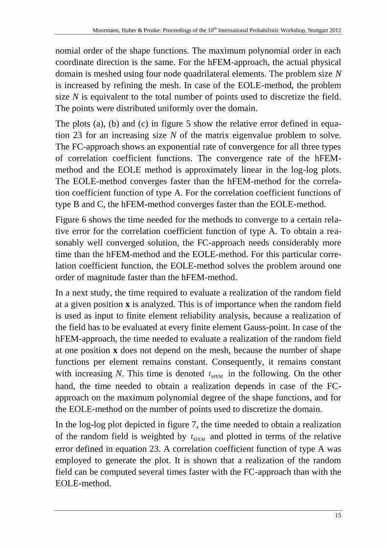
In the log-log plot depicted in figure 7, the time needed to obtain a realization
of the random field is weighted by hFEMt and plotted in terms of the relative
error defined in equation 23. A correlation coefficient function of type A was
employed to generate the plot. It is shown that a realization of the random
field can be computed several times faster with the FC-approach than with the
EOLE-method.
Betz; Papaioannou; Straub: A finite cell approach for discretization of random fields
16
1
10
100
1000
0.0001 0.001 0.01 0.1 1
tim
e/t
_h
FE
M
relative error
FC
EOLE
Figure 7. Time needed to compute a realization of the random field. Comparison between
FC-approach and EOLE-method. Time is given relative to the time needed with the hFEM-
method.
4 Summary and Conclusion
The proposed FC-approach exhibits an exponential rate of convergence with
respect to the mean error variance. However, it is relatively expensive to
compute a random field approximation. This effect will be even more severe
for three-dimensional problems. On the other hand, compared to the EOLE-
method, the proposed approach is computationally very efficient in obtaining
a random field realization. This is advantageous, if many realizations of the
random field have to be generated.
Compared to the hFEM method, the proposed approach is computationally
more expensive in obtaining a random field realization. Therefore, for do-
mains which are meshed with a linear finite element mesh that is fine enough
to represent the correlation structure of the random field reasonably well, the
hFEM-method is to be preferred. However, the FC-approach is useful for
problems that do not require a mesh on the physical domain, e.g. meshless
approaches or FC methods.
References
[1] Betz, W.: Quasi meshless discretization of random fields based on the Karhunen-
Loève expansion. TU München, 2012 – Master’s thesis
[2] Ditlevsen, O.; Madsen, H.O.: Structural Reliability Methods. Chichester: John Wiley
& Sons Ltd, 1996
[3] Düster, A.; Parvizian, J.; Yang, Z.; Rank, E.: The finite cell method for three-
dimensional problems of solid mechanics. Comp. Methods Appl. Mech. Engrg. 197
(2008), p. 3768-3782

Moormann, Huber & Proske: Proceedings of the 10th International Probabilistic Workshop, Stuttgart 2012
17
[4] Ghanem, R.-G.; Spanos, P.-D.: Polynomial chaos in stochastic finite elements.
Applied Mechanics 57 (1990), p. 197-202.
[5] Ghanem, R.-G.; Spanos, P.-D.: Stochastic Finite Elements - A Spectral Approach.
New York: Springer, 1991
[6] Li, C.-C.; Der Kiureghian, A.: Optimal discretization of random fields. Journal of
Engineering Mechanics 119 (1993), p. 1136-1154
[7] Papaioannou, I.: Non-intrusive Finite Element Reliability Analysis Methods. TU
München, 2012 – Dissertation
[8] Parvizian, J.; Düster, A.; Rank, E.: Finite cell method. Computational Mechanics
41 (2007), p. 121-133
[9] Sudret, B.; Der Kiureghian, A.: Stochastic finite element methods and reliability
– a state-of-the-art report. Technical Report UCP/SEMM-2000/08, Department of
Civil & Environmental Engineering, Univ. of California, Berkeley, November 2000
[10] Sudret, B.: Uncertainity propagation and sensitivity analysis in mechanical models -
Contributions to strucutral reliability and stochastic spectral methods. Université
BLAISE PASCAL - Clermont II, 2007 – Habilitation.
[11] Szabó, B. A.; Düster, A.; Rank, E.: The p-version of the finite element method. In:
Stein E, de Borst R, Hughes TJR (eds) Encyclopedia of computational mechanics,
Vol. 1, Chapter 5. Wiley, New York (2004), pp. 119–139

Betz; Papaioannou; Straub: A finite cell approach for discretization of random fields
18

Moormann, Huber & Proske: Proceedings of the 10th International Probabilistic Workshop, Stuttgart 2012
19
Bayesian estimation of the covariance function
of random fields based on a limited number of
measurements
Pieterjan Criel, Robby Caspeele, Luc Taerwe
Magnel Laboratory for Concrete Research, Ghent University, Ghent
Abstract: A Bayesian response surface updating procedure is applied in order
to update covariance functions for random fields based on a limited number of
measurements. Formulas as well as a numerical algorithm are presented in or-
der to update the parameters of complex response surfaces using Markov Chain
Monte Carlo simulations. In case of random fields, the parameters of the covar-
iance function are often based on some kind of expert judgment. However, a
Bayesian updating technique enables to estimate the parameters of the covari-
ance function more rigorously and with less ambiguity. Prior information can
be incorporated in the form of vague or informative priors, and the latter can be
based on e.g. expert judgment. The proposed estimation procedure is evaluated
through numerical simulations and the influence of the position of measure-
ment points is investigated.
1 Introduction
The parameters of the covariance function of random fields are often based on some kind
of expert judgment, certainly in cases where only a few measurements are available. How-
ever, Bayesian updating techniques enable to estimate the parameters of the covariance
function more rigorously and with less ambiguity as these can be used to update previously
obtained information regarding parameters of similar random fields. Markov chain Monte
Carlo (MCMC) simulations can be used to incorporate Bayesian updating based on limited
samples in the response surface estimation. Prior information (vague or informative) can
then be used to update the covariance function based on available monitoring data or
measurement results. Of course, the sample pattern according to which the measurements
are obtained plays an important role for optimizing the Bayesian estimation method in case
only a few measurements can be obtained.
Criel, Caspeele & Taerwe: Bayesian estimation of the covariance function of random fields based on a limited number of
measurements
20
2 Random fields and their covariance function
A random field xH is a function whose values are random variables for any
position x . In general, their characteristics can differ for each position x in
the random field. Some of the phenomena that can be represented by random
fields are: the bathymetry of the sea, the earth’s surface temperature, concrete
properties in structural elements, etc. resulting from a distributed disordered
system that displays complex patterns of variation in space and/or time [15].
For numerical applications random fields are most often defined on a discrete
domain, e.g. on a lattice grid (lattice process). A continuous random field can
be obtained by interpolation methods, e.g. Kriging [3]. In many cases the ran-
dom field is defined on a surface and can be decomposed into a mean value or
trend surface and a residual variation with mean 0. This residual variation
usually exhibits some spatial structure, described by a covariance function ),( ji xxC . The covariance function is a measure of the correlation between
two positions in the field. When a random field is considered to be homoge-
neous, isotropic and ergodic the covariance function is only dependent on the
distance between two positions in the field, hence:
)(),( CxxC ji (1)
Random fields are called Gaussian if the random variables which describe the
field follow a Gaussian distribution. An advantage of such fields is that they
can be transformed into a field described by standard normal distributed vari-
ables. As such, further in this paper only standard normal distributed random
fields need to be considered.
A standard normal field is characterized by its mean 0 and its covariance
function and can be presented by a multivariate standard normal distribution:
HHf TN
H12/12/
2
1exp2 (2)
where N is the amount of positions x in the field, the mean value of the
field and the covariance matrix, whose elements ji, are equal to the co-
variance between position ix and jx :
Moormann, Huber & Proske: Proceedings of the 10th International Probabilistic Workshop, Stuttgart 2012
21
),( jiij xxC (3)
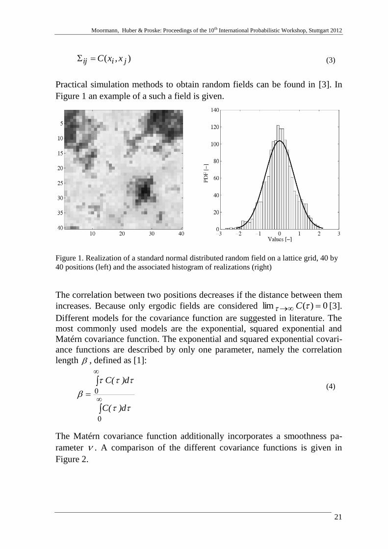
Practical simulation methods to obtain random fields can be found in [3]. In
Figure 1 an example of a such a field is given.
Figure 1. Realization of a standard normal distributed random field on a lattice grid, 40 by
40 positions (left) and the associated histogram of realizations (right)
The correlation between two positions decreases if the distance between them
increases. Because only ergodic fields are considered 0)(lim C [3].
Different models for the covariance function are suggested in literature. The
most commonly used models are the exponential, squared exponential and
Matérn covariance function. The exponential and squared exponential covari-
ance functions are described by only one parameter, namely the correlation
length , defined as [1]:
0
0
d)(C
d)(C
(4)
The Matérn covariance function additionally incorporates a smoothness pa-
rameter . A comparison of the different covariance functions is given in
Figure 2.
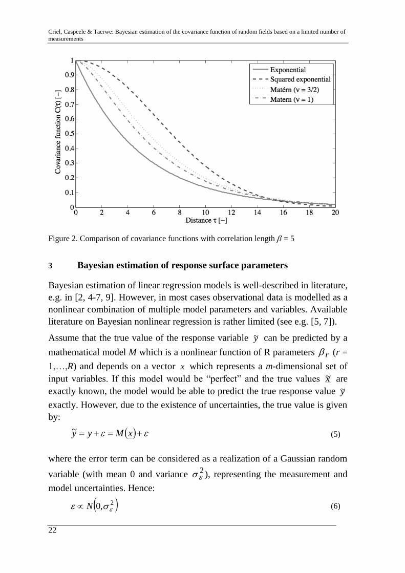
Criel, Caspeele & Taerwe: Bayesian estimation of the covariance function of random fields based on a limited number of
measurements
22
Figure 2. Comparison of covariance functions with correlation length = 5
3 Bayesian estimation of response surface parameters
Bayesian estimation of linear regression models is well-described in literature,
e.g. in [2, 4-7, 9]. However, in most cases observational data is modelled as a
nonlinear combination of multiple model parameters and variables. Available
literature on Bayesian nonlinear regression is rather limited (see e.g. [5, 7]).
Assume that the true value of the response variable y~ can be predicted by a
mathematical model M which is a nonlinear function of R parameters r (r =
1,…,R) and depends on a vector x which represents a m-dimensional set of
input variables. If this model would be “perfect” and the true values x~ are
exactly known, the model would be able to predict the true response value y~
exactly. However, due to the existence of uncertainties, the true value is given
by:
xMyy~ (5)
where the error term can be considered as a realization of a Gaussian random
variable (with mean 0 and variance 2 ), representing the measurement and
model uncertainties. Hence:
2,0 N (6)
Moormann, Huber & Proske: Proceedings of the 10th International Probabilistic Workshop, Stuttgart 2012
23
where the variance of the error term is assumed to be constant in the domain
of the input variables.
If N independent test results iy are available for the response variable of N
sets of corresponding input variables ix , the likelihood of the experimental
data can in general be written as:
Nii
RNi
xMy,...,,y,...,yL
1
111
(7)
where . is the probability density function (PDF) of the standard normal
distribution.
Based on the Bayesian principle, the prior information (either vague or in-
formative) is given as the joint prior distribution RB ,...,,f 1 of the
standard deviation of the error term and the model parameters R,...,1 .
This prior distribution can be updated towards a posterior distribution
RB ,...,,f 1 by using the likelihood function as follows:
RNRB
BRRNRB
RNRB
RB
,...,,y,...,yL,...,,fc
d...dd,...,,y,...,yL,...,,f
,...,,y,...,yL,...,,f
,...,,f
111
1111
111
1
(8)
with c a normalizing constant and B the domain of the parameters
R,...,, 1 that have to be updated. Equation (8) can be difficult or im-
possible to solve analytically. Therefore MCMC simulations are applied (i.e.
using the Metropolis-Hastings algorithm) to estimate values for the model
parameters and the standard deviation of the error term.
4 MCMC Bayesian updating of response surface parameters using a
‘cascade’ Metropolis-Hastings algorithm
Markov chain Monte Carlo methods (MCMC) form a class of numerical algo-
rithms that allow to obtain samples from probability distributions based on the
construction of a Markov chain. A Markov chain is defined in probability
theory as a sequence of random variables xi for which the distribution of xi,
Criel, Caspeele & Taerwe: Bayesian estimation of the covariance function of random fields based on a limited number of
measurements
24
conditioned on past realizations xi-1, xi-2, …, depends only on the previous
sample xi-1, i.e. not on xi-2, xi-3, etc. [5]. Thus, these methods allow to draw a
discrete-time homogeneous chain of samples from the posterior distribution
[13]. The idea is to generate iteratively samples of a Markov chain, which
asymptotically behaves as the probability density function (PDF) which has to
be sampled. More specifically, the Metropolis-Hastings algorithm [8, 12] is
commonly used for generating such Markov chains. The practical adaptation
of this algorithm for the Bayesian estimation of response surface parameters
is explained hereafter. More profound information on MCMC simulations can
be found in e.g. [4-6, 10, 14].
Considering a certain PDF xf X which is a function of an input vector x ,
MCMC realizations sx are generated sequentially and independently, starting
from an arbitrary chosen starting vector 0x . In each step, the transition be-
tween the states sx and 1sx is given according to (see e.g. [5]):
else
y probabilit with 1
s
sss
x
x~,xxx~qx~x
(9)
where x~ is a candidate vector, sxx~q is called the transition or proposal dis-
tribution and the acceptance probability x~,xs given by (see e.g. [5]):
s
s
sX
Xs
xx~q
x~xq
xf
x~f,minx~,x 1 (10)
Practically, in order to select a candidate x~ – calculated according to Equa-
tion (5) – a random number rs is generated (i.e. from a uniform distribution
U[0;1]) and x~ is accepted as the next draw from xf X with a probability
x~,xs in case x~,xr ss or rejected in the other case. This way, a se-
quence of random draws sx from xf X is generated, even when no analyti-
cal solution is available for xf X .
By using the random walk algorithm to propose values for the parameters the
transition distribution is symmetrical and Equation (10) can be simplified to:
sX
Xs
xf
xfxx
~,1min~, (11)
Moormann, Huber & Proske: Proceedings of the 10th International Probabilistic Workshop, Stuttgart 2012
25
In case of the Bayesian estimation of response surface parameters, the transi-
tion between 2 estimates s,Rs,s, ,...,, 1 and 1111 s,Rs,s, ,...,,
for the posterior set of response surface parameters can be rewritten as:
else
,...,,
y probabilit with
,...,,~
,...,~
,~~,...,
~,~
,...,,
,,1,
,,1,11
1,1,11,
sRss
sRssRR
sRss
q
(12)
where s,Rs,s,R ,...,,~
,...,~
,~q 11 is the transition distribution. A com-
mon choice for the transition distribution is a random walk, more specifically
by adding a random increment to the previous estimate according to:
TRT
s,Rs,s,T
R ,...,,,...,,~
,...,~
,~ 1011 (13)
with R,...,, 10 a random vector that does not depend on the previous
chain. In practice, it is common to choose the values i according to a normal
or uniform distribution with mean 0 and variance 2 . The latter value deter-
mines how fast the MCMC algorithm will converge to yield the posterior
response surface parameters.
Further, the probability is the joint acceptance probability based on the
prior probability and the likelihood function or in other words the probability
that a random sample 10;UuP from a uniform distribution (defined for
values between 0 and 1) is accepted according to the prior distribution and
that a random sample 10;UuL is accepted according to the likelihood
function. Based on the “cascade” principle as described in [2,7], this probabil-
ity is generalized for Bayesian estimation of response surface parameters ac-
cording the following equations:
LLPP uu Prob (14)
s,Rs,s,B
RB
Rs,Rs,s,PP
,...,,f
~,...,
~,~f
,min
~,...,
~,~,,...,,
1
1
11
1 (15)
Criel, Caspeele & Taerwe: Bayesian estimation of the covariance function of random fields based on a limited number of
measurements
26
sRssN
RN
RsRssLL
yyL
yyL
,,1,1
11
1,,1,
,...,,,...,
~,...,
~,~,...,
,1min
~,...,
~,~,,...,,
(16)
with the likelihood ...y,...,yL N1 according to Equation (7) in case of se-
quentially independent response measurements.
5 Bayesian estimation of the covariance function based on limited
measurements
Consider a random field with an exponential or a squared exponential covari-
ance function. In this case there is only one parameter which has to be esti-
mated, namely the correlation length . Instead of fitting a covariance
function to an empirical covariance function, it is fitted to a semi-variogram.
A semi-variogram ji xx , or variogram ji xx ,2 is – like the covariance
function – a function describing the degree of spatial dependence in a random
field. It is defined as the variance of the difference between two values of the
field. For homogeneous and isotropic fields the semi-variogram is only de-
pending on the distance between those two positions, hence:
22,2 jiji xxxx (17)
For second order stationary random fields the following relation between the
semi-variogram en the covariance function holds [3]:
CC 022 (18)
with the semi-variogram and C a covariance function.
The semi-variogram has the advantage that the mean value of the field - as-
sumed constant (if necessary after a trend correction) - does not have to be
known to compose the empirical semi-variogram.
This strategy is also applied in other methods for estimating the correlation
length based on measurement data, e.g. the maximum likelihood estimation
(MLE) and the least squares method (LSQ) [3]. However, these methods do
not consider prior information on the covariance function, i.e. prior infor-
mation on the correlation length . As such, the bias and uncertainty of the
Moormann, Huber & Proske: Proceedings of the 10th International Probabilistic Workshop, Stuttgart 2012
27
estimation can be very large in case of limited data. When considering prior
knowledge this can however be ameliorated. The method presented in section
4 can be applied to update the model parameters of the covariance function
based on a limited amount of measurements considering the empirical semi-
variogram derived from the measurements. Prior informative is given as the
joint distribution (either vague or informative) of the error term and the pa-
rameters that define the covariance function. In case a uniform distribution is
assumed for the error term and lognormal distributions for the correlation
length, the prior distribution becomes:
with and the parameters of the lognormal distribution.
Rewriting Equation (5) in terms of the semi-variogram yields:
| (20)
where is the empirical semi-variogram, | the semi-variogram
model and the error term as defined in Equation (6).
There are different methods commonly available to compose an empirical
semi-variogram based on measurement data [3]. In this paper the method-of-
moments estimator defined by Matheron [11] is adopted:
)(2
2
1
T ji hhT
(21)
NjihhhhT jiji ,,1,;:, (22)
where T is a set defined by Equation (22), T is the number of elements
in the set T (i.e. the number of available measurements for a certain dis-
tance ) and ji hh , are the values of the measurements. Other methods can be
found in [3].
else 0
b a if 2
1
2
112
lnexp
ab
,'f
(19)
Criel, Caspeele & Taerwe: Bayesian estimation of the covariance function of random fields based on a limited number of
measurements
28
is not continuous as there are only a finite number of distances between
the measurement points. In order to obtain sufficient samples per set T for
constructing a semi-variogram in practice, similar distances are grouped in
distance classes by adding a tolerance on the distance . Hence, the set of el-
ements corresponding to a distance class are described as follows:
The tolerance e should be carefully chosen so that the empirical semi-
variogram is not biased and there are enough combinations available in each
distance class.
In the case of an exponential covariance function (i.e. with two unknown pa-
rameters, namely the correlation length and the standard deviation of
the error term), the likelihood function defined in Equation (7) in terms of the
semi-variogram can be rewritten as:
Nii
Ni
L1
|
2
1exp
2
1,,...,
21
(24)
By using a symmetrical transition distribution the simplified acceptance prob-
ability can be used in the MCMC simulation. The acceptance probabilities
P and L as given in Equation (14) and (15) respectively can then be re-
written as:
s,
P,'f
~,~
'f,min
s
1 (25)
N
2s,
sii
s,
N
2ii
L
i
|exp
i ~
~|
exp~
,min
1 2
1
2
1
1 2
1
2
1
1
(26)
As an example the traditional LSQ method and the currently developed
MCMC method are compared. Both methods (MCMC method based on 25
measurement points on a domain of 32 x 32 positions and LSQ method based
on 25 or 1024 measurement points on the same domain size) are applied to
NjiehhehhT jiji ,,1,;:, (23)
Moormann, Huber & Proske: Proceedings of the 10th International Probabilistic Workshop, Stuttgart 2012
29
find the correlation length of a random field on a lattice grid (40 by 40 po-
sitions). For each method 100 standard normal distributed random fields with
a correlation length = 10 are generated. In case of the MCMC method a
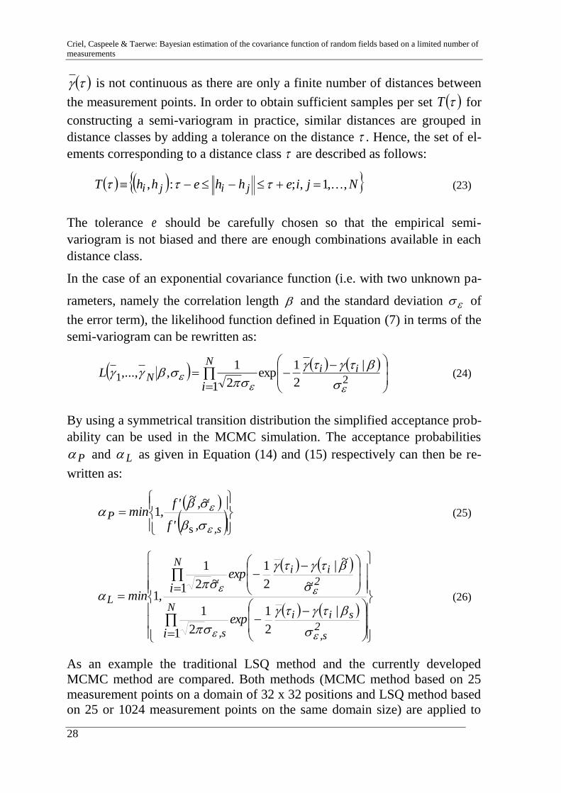
lognormal prior distribution for is considered with 8 and 2 . The results are shown in Figure 3. Hence, the prior distribution used for the
correlation length was biased. Figure 3(C) shows the prior and posterior PDF
of the correlation length in case of the MCMC method.
Compared to the LSQ method, the MCMC method provides a less uncertain
estimation (due to the incorporation of prior information). The LSQ estima-
tion improves when more measurement points are available, however a large
number of measurement points are necessary for achieving a similar accuracy
as provided by the MCMC method. 1024 or more measurement points are of
course impossible to achieve in common structural engineering applications,
hence indicating the importance of the proposed MCMC method.
Figure 3. (A) Probability density function (PDF) of in case of the LSQ method consider-
ing 1024 measurement points. (B) PDF of in case of the LSQ method considering 25
measurement points. (C) PDF of in case of the MCMC method considering 25 meas-
urement points and prior information. (D) 90% confidence intervals for the LSQ and
MCMC method when considering 25 points. (E) 90% confidence interval for the LSQ
method when considering 1024 points compared to the MCMC method when considering
25 points.
Criel, Caspeele & Taerwe: Bayesian estimation of the covariance function of random fields based on a limited number of
measurements
30
6 Study of the influence of the sample pattern
In order to optimize the information which can be obtained from a limited
number of measurement points, the sample pattern according to which the
measurements are obtained plays an important role for the efficiency of the
Bayesian estimation method. Two patterns are considered in the following,
namely patterns with a constant distance between the measurement points
(linear regular pattern) and a pattern where de distance between the measure-
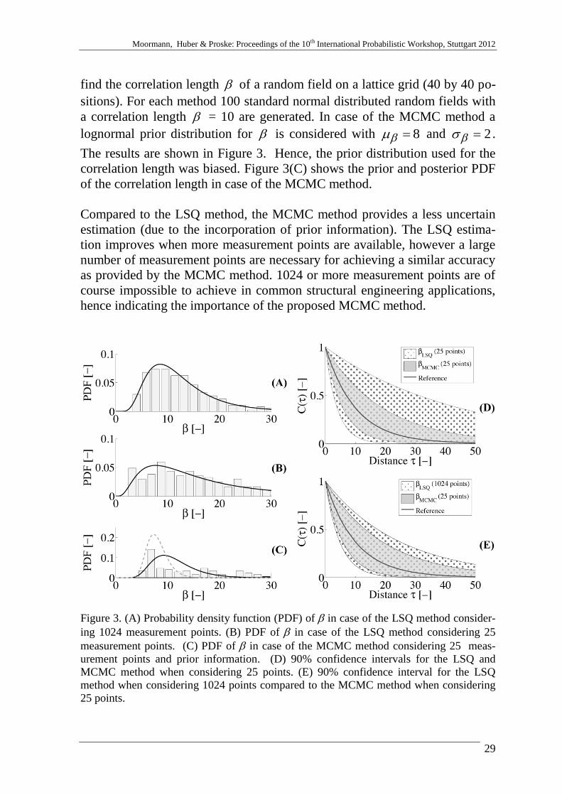
ment points grows exponentially (logarithmic regular pattern), see Figure 4.
Figure 4. Linear regular pattern (left) and logarithmic regular pattern (right)
For the linear regular pattern a larger amount of measurement couples per dis-
tance class are available, while in case of the logarithmic regular pattern a
larger amount of different distance classes is represented, although less meas-
urements per distance class are available. A linear regular pattern will have
the advantage that there are more measurements available for each distance
class, while the logarithmic pattern samples according to a larger number of
distance classes. However, in the latter case less measurement points are
available per distance class, which leads to a less informative likelihood func-
tion.
In order to compare the influence of both sample patterns, the performance of
the MCMC method for estimating the correlation length of a standard
normal random field defined on a lattice grid (40 by 40 positions) is quanti-
fied for a specific example. For both suggested sample patterns 100 standard
normal distributed random fields with a correlation length 10 are generat-
ed. A lognormal prior distribution for is considered with 10 and
2 . In case 25 measurement points are considered according to both
Moormann, Huber & Proske: Proceedings of the 10th International Probabilistic Workshop, Stuttgart 2012
31
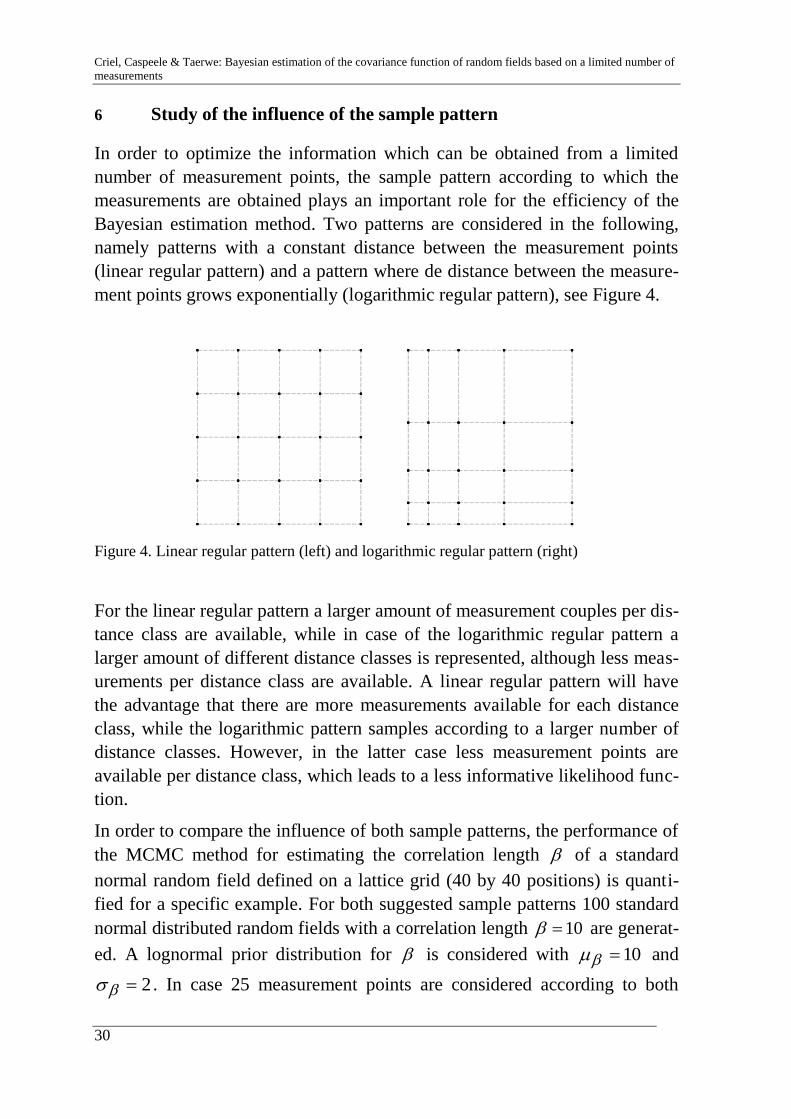
sample patterns over the same domain (15 by 15 positions), the results are
shown in Figure 5.
Figure 5. PDF of for the logarithmic and linear pattern (left) and 90% confidence interval
for the logarithmic and linear pattern (right)
From Figure 5 it can be concluded that in case the prior information is con-
sistent with the simulation reference and the sample patterns have the same
span, a more informative likelihood function is obtained according to a linear
sample pattern (as discussed above), which consequently results in a smaller
confidence interval of the estimated correlation length.
7 Conclusions
By assuming homogeneous, isotropic and ergodic properties for ran-
dom fields, the spatial characteristics are determined by the covariance
function.
A methodology based on Markov chain Monte Carlo (MCMC) simula-
tions is developed in order to estimate the covariance function of ran-
dom fields from empirical semi-variograms and considering Bayesian
updating of prior information.
When only a limited amount of measurement data is available, the
MCMC method enables to obtain a more accurate estimation of the cor-
relation length of random fields compared to the commonly used LSQ
method.
With respect to constructing a semi-variogram, the use of a linear sam-
ple pattern results in a smaller confidence interval for the estimated cor-
Criel, Caspeele & Taerwe: Bayesian estimation of the covariance function of random fields based on a limited number of
measurements
32
relation length in case the prior information is consistent with the simu-
lation reference and the sample patterns have the same span.
8 References
[1] Baecher, G.B. and J.T. Christian, Reliability and Statistics in
Geotechnical Engineering. 2003: John Wiley & Sons.
[2] Box, G.E.P. and G.C. Tiao, Bayesian inference in statistical analysis.
1992: Wiley.
[3] Cressie, N.A.C., Statistics for spatial data. 1993: J. Wiley.
[4] Gamerman, D. and H.F. Lopes, Markov Chain Monte Carlo: Stochastic
Simulation for Bayesian Inference, Second Edition. 2006: Taylor &
Francis.
[5] Gelman, A., et al., Bayesian Data Analysis. 2003: Chapman &
Hall/CRC.
[6] Ghosh, J.K., M. Delampady, and T. Samanta, An Introduction to
Bayesian Analysis: Theory and Methods. 2010: Springer.
[7] Gregory, P., Bayesian Logical Data Analysis for the Physical Sciences:
A Comparative Approach with Mathematica® Support. 2005:
Cambridge University Press.
[8] Hastings, W.K., Monte Carlo sampling methods using Markov chains
and their applications. Biometrika, 1970. 57(1): p. 97-109.
[9] Lee, P.M., Bayesian Statistics: An Introduction. 2012: Wiley.
[10] Liu, J.S., Monte Carlo Strategies in Scientific Computing. 2008:
Springer.
[11] Matheron, G., Traité de géostatistique appliquée. Technip ed. Vol. 14.
1962, Paris.
[12] Nicholas, M., et al., Equation of State Calculations by Fast Computing
Machines. The Journal of Chemical Physics, 1953. 21(6): p. 1087-
1092.
[13] Perrin, F., et al. Comparison of Markov chain Monte Carlo simulation
and a FORM-based approach for Bayesian updating of mechanical
models. in 10th int. Conf. on Applications of Statistics and Probability
in Civil Engineering. 2007. Tokyo: Taylor & Francis Group.
[14] Robert, C. and G. Casella, Monte Carlo Statistical Methods. 2010:
Springer.
[15] VanMarcke, E., Random Fields: Analysis and Synthesis. 2010: World
Scientific.
Moormann, Huber & Proske: Proceedings of the 10th International Probabilistic Workshop, Stuttgart 2012
33
Assessing the prediction quality of coupled partial models considering coupling quality
Holger Keitel Research Training Group 1462, Bauhaus-Universität Weimar,
Berkaer Str. 9, 99423 Weimar, Germany
Abstract: The process of analysis and design in structural engineering requires the consideration of different partial models of loading, structural material, structural elements, and analysis type, among others. The various partial mod-els are combined by coupling of their several components. Due to a large num-ber of available partial models describing similar phenomena many different model combinations are possible to simulate the same quantities of a structure. The challenging task of an engineer is to select a model combination that en-sures a sufficient reliable prognosis. In order to achieve this reliable prognosis of the overall structural behaviour, on the one hand a high individual quality of the partial models and on the other hand an adequate coupling of the partial models is needed. Several methodologies have been proposed so far to evaluate the quality of partial models for their intended application, but a detailed study of the coupling quality is still lacking. This paper proposes a new approach to assess the quality of coupled partial models in a quantitative manner taking into account directly the coupling quality. In order to achieve a global measure for the quality of the coupled partial models existing methods based on graph theo-ry and variance based sensitivity analysis are extended to include the quality of coupling. The functionality of the algorithm is demonstrated using an example of structural engineering.
1 Introduction
The models used in structural engineering to design for serviceability and the ultimate limit state are composed of several partial models (PM) and their couplings (C). A partial model describes a component of the global model, e.g. loading, material, or the level of abstraction. For each class of PMs, e.g. the material behavior of steel, several possibilities of modeling are available. If the material model is relevant for the structural behavior, the structural en-gineer needs to decide, whether a linear or a non-linear material model should
Keitel: Assessing the prediction quality of coupled partial models considering coupling quality
34
be used and whether further effects, e.g. long-term behavior, have to be con-sidered. Apart from the selection of appropriate partial models the coupling of the individual PMs is a key issue. Some partial models might interact with each other, thus a coupling is substantial and the quality of this coupling in-fluences the quality of the global model.
In recent years, strategies to estimate the quality of partial models, [4], [5], and to quantify the influence of the partial models on the global model prog-nosis [3] have been developed. Furthermore, the quantification of the progno-sis quality of a global model, neglecting the influence of coupling quality, is described in [3]. The assessment of software coupling has been shown in [1], but does not apply to partial models directly. Altogether, the evaluation of partial model coupling and its influence on the prognosis of a global model has not been addressed so far.
In the scope of this paper a method to quantify the quality of data coupled partial models is presented. The basis of the procedure is the consistency of data belonging to the coupled partial models. Besides the pure data integrity the influence of the coupling on the partial models’ output is taken into ac-count within the framework of the evaluation algorithm. Further, a quantita-tive measure for the prediction quality of the global model taking into account the individual qualities of the partial models, their influence on the output quantity, and coupling quality is derived.
2 Basic Methods and Principles
2.1 Graphical Representation of Coupled Partial Models
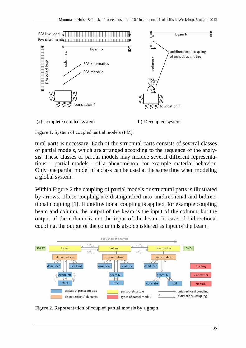
Global models used in engineering consist of several partial models. Figure 1 depicts a structure of a simply supported beam, connected to a clamped col-umn with a footing. Exemplarily several partial models are shown. On the left side the overall structure is presented all in one, on the right side the structural parts are decoupled.
Stein, Lahmer, and Bock [8] show that a global model can be represented schematically by a graph, consisting of vertices – symbolizing the partial models – and edges – symbolizing the coupling. This idea is extended within the scope of this paper. The global model in Figure 1, represented by the graph in Figure 2, is separated into its structural components; beam, column, and foundation. Due to the numerical calculation, a discretization of the struc
Moormann, Huber & Proske: Proceedings of the 10th International Probabilistic Workshop, Stuttgart 2012
35
(a) Complete coupled system (b) Decoupled system
Figure 1. System of coupled partial models (PM).
tural parts is necessary. Each of the structural parts consists of several classes of partial models, which are arranged according to the sequence of the analy-sis. These classes of partial models may include several different representa-tions – partial models - of a phenomenon, for example material behavior. Only one partial model of a class can be used at the same time when modeling a global system.
Within Figure 2 the coupling of partial models or structural parts is illustrated by arrows. These coupling are distinguished into unidirectional and bidirec-tional coupling [1]. If unidirectional coupling is applied, for example coupling beam and column, the output of the beam is the input of the column, but the output of the column is not the input of the beam. In case of bidirectional coupling, the output of the column is also considered as input of the beam.
Figure 2. Representation of coupled partial models by a graph.
Keitel: Assessing the prediction quality of coupled partial models considering coupling quality
36
2.2 Sensitivity Analysis applied to Partial Models
Sensitivity analyses quantify the influence of input parameters on the output of a model. As proposed in [3], variance-based global sensitivity analysis can also be used to study the influence of partial models on the output of the glob-al model. This procedure detects the most influential classes of partial models. Consequently, when evaluating the quality of the global model, the individual quality of the partial models with high influences on the system’s behavior is crucial for the overall prognosis quality. This algorithm to quantify the influ-ence of classes of partial models is the basis of this investigation of coupling quality as well as total prediction quality and is described in the following.
Each of the classes of partial models i, j is represented by a uniformly distrib-uted, discrete random parameter
{ } { },...0,1,0,1 ∈∈ ji XX (1)
A value of Xi=0 denotes the deactivated partial model class i, for example ge-ometric non-linearity is not included, and Xi=1 denotes the activated partial model class i. The global model Y is calculated for all possible combinations of the number of Np partial model classes. Using these model results all re-quired sensitivity indices can be calculated.
The exclusive influence of the parameter Xi is quantified by the first-order sensitivity index Si, defined in detail in [7].
In order to take into account coupling effects, the total-effects sensitivity in-dex STi was introduced by Homma and Saltelli [2]. Besides the exclusive in-fluence of the parameter Xi on the variance of the response, the STi index considers the interaction of Xi with all other parameters X~i. These interactions are quantified by the difference of Si and STi. Further, when using high-order indices Sij, these interactions can be directly apportioned to specific parame-ters/classes i and j of partial model. For details see [6].
In the present case of discrete input parameters all first-order, total-effects, and high-order indices can be calculated directly from the results of model Y for the N combinations of input parameters without the usual need of specific sensitivity estimators, which require high computational effort.
Moormann, Huber & Proske: Proceedings of the 10th International Probabilistic Workshop, Stuttgart 2012
37
3 Coupling Quality
3.1 Quality of Data Coupling
Within the scope of this paper, coupling is defined as data coupling and the quality of coupling is related to the quality of data transfer. Let α and β be quantities appearing in both partial models k and l at the same point on the structure, for example forces or displacements. A perfect data coupling en-sures consistent data in both models, e.g. αk=α l, which refers to data coupling quality of cqf
α,k-l=1. The index f denotes the forward coupling according to the sequence of partial models within the graph, whereas b denotes the backward-coupling, for example cqb
β,l-k. As the differences in transferred data increases, the quality of the coupling decreases down to a quality of zero when no data is transferred. This leads to the following definition of data coupling quality:
{ } and ,max
1f, lk
lk
lkcqαα
ααα
−−=− { }.,max
1, lk
lkb
klcqββ
βββ
−−=− (2)
The data coupling quality depends on the quantity being compared. As a coupling might consist of numerous data, the mean quality of Nf forward and Nb backward transferred data is derived with
and 11
f,∑
=−− =
fN
lkf
f
lk cqN
cqα
α .11
,∑=
−− =bN
bkl
b
b
kl cqN
cqβ
β (3)
An example of coupling is the data transfer of the support forces of the column to the foundation in Figure 1, when both structural parts are analyzed seperately. The forward quantities normal force, shear force, and bending moment are transferred to the foundation, and the backward quantities deformation in vertical direction uz and horizontal direction ux as well as the rotation ϕy, that occur due to the flexibility of the soil, are transferred back to the column support and are considered pre-deformations of the column at the support.
Keitel: Assessing the prediction quality of coupled partial models considering coupling quality
38
3.2 Influence of Coupling on Data
Independent from the quality of data coupling, the question of the influence of coupling on the data needs to be answered. For this reason, variance-based sensitivity analysis according to Section 2 is applied. In the current section the sensitivity of the forward coupled data quantities with respect to the partial models is explored, which is in contrast to the usual algorithms used when the sensitivity of certain structural quantities of the global system is determined.
For this analysis the partial models need to be distinguished based on their position in the sequence of the analysis: partial models arranged before the investigated coupling, denoted as PM≤k, and models arranged after the inves-tigated coupling, denoted as PM≥l. If the coupling quality of column-foundation needs to be determined for the graph in Figure 2, PM≤k refers to all models directly linked to the beam and the column, and PM≥l refers to all models directly linked to the foundation.
Using high-order indices, the influence of partial models on the transferred data can be apportioned to each model and to several groups of models. In the present case we are interested in the sensitivity of the transferred data with respect to all PM≤k and all PM≥l. The sum of high-order indices for the groups of models becomes
. and 1
,,.
∑∑∑∑∑∑≤=≥≤ ≤≤
−==kPM
N
iTi
lPMki kjij
kPM
SSSSSp
ααααα (4)
In ∑≤kPM
Sα no first-order or higher-order indices referring to any PM≥l are in-
cluded. This value is a measure of the importance of forward coupling for quantity α. In contrast to this, ∑
≥lPMSα indicates the importance of backward
coupling and includes all first-order for PM≥l and all high-order terms refer-ring to any PM≥l. The need for bidirectional coupling increases with an in-creasing influence of backward coupling. Hence, the coupling quality is more and more dependent on the quality of the backward coupling.
3.3 Quality of Partial Model Coupling
In order to derive the quality of PM coupling, the data coupling quality and the influence of coupling are combined. The final application of the derived
Moormann, Huber & Proske: Proceedings of the 10th International Probabilistic Workshop, Stuttgart 2012
39
coupling quality is the consideration within the framework of model evalua-tion, thus the quality of coupling is defined with this motive. In order to do so, the coupling quality depends on the position of the output quantity in the graph, for which the influence of coupling is investigated for.
When the coupling quality is evaluated for coupled PMs that are after the in-vestigated output quantity in the sequence of the analysis, a backward cou-pling is essential; otherwise no information of the partial models arranged after the coupling can be transferred back to the PMs that are before in the sequence of the analysis. In this case, quality of coupling becomes
.b
kl
f
lklk cqcqCQ −−− ×= (5)
If one of the forward or backward data coupling quality is zero, the total qual-ity is zero as well.
When coupling quality is evaluated for coupled PMs that are arranged before the investigated output quantity, the backward coupling might influence the coupled quantities to some extent, but it is not obligatory. In this case the quality is defined as
.1
11
1
11,
∑∑
∑ ∑∑ ∑
=
= ≥−
= ≤−
−
⎟⎠
⎞⎜⎝
⎛+⎟
⎠
⎞⎜⎝
⎛
=
PM
N
f
N
lPMf
b
kl
N
kPM
flk
flk
SN
SN
cqScqN
CQf
ff
f
αα
αα
ααα
(6)
The forward data coupling quality cqfα is directly linked to the sensitivity in-
dices of α. For backward data coupling quality this is not possible, because it cannot be determined which of the backward coupling quantities β has an in-fluence on α. Furthermore, the number of forward and backward coupling quantities might differ. Hence, the mean value of sensitivity indices of α is multiplied with the mean of backward data coupling quality .
b
klcq −
3.4 Global Model Quality
The prediction quality of the global model for an output quantity γ depends on the quality of partial models, their influence on the quantity of interest, and
Keitel: Assessing the prediction quality of coupled partial models considering coupling quality
40
the coupling quality. The quality of partial model i, MQi, is weighted by the influence of partial model i on quantity γ, quantified by SγTi, with respect to the sum of all SγTi of the NPM partial models involved. In addition, the quality contribution of each partial model is multiplied by coupling quality, CQc, of each of the Nc,i,γ couplings that are necessary to transfer data from PMi to the quantity of interest γ. For example, to transfer data from the beam to the foundation, Figure 1 and 2, two couplings, beam-to-column and column-to-foundation, are necessary. This means, Nc,i,γ is equal to two. The resulting model quality of the global model GM for quantity γ becomes
.1 1
1
,,
∑ ∏∑= =
=⎥⎥
⎦
⎤
⎢⎢
⎣
⎡=
PM ic
PMGM
N
i
N
cciN
j Tj
Ti CQMQS
SMQγ
λ
γγ (7)
The coupling quality CQc of the partial models a and b being coupled is once more distinguighed into two cases, depending on the position of the output quantity γ within the sequence of the graph:
⎩⎨⎧
=−
−
).with(couplingcouplingbeforeisif)with(couplingcouplingafterisifbacCQ
bacCQCQ b
ba
aba
c γγ
(8)
4 Example
4.1 Partial Models and First Results
In the following, an example depicted in Figure 3 is analyzed with respect to coupling quality and the total prediction quality. The considered partial mod-els are: live load beam (PM1), non-linear material behavior of the steel col-umns (PM2), geometric non-linear behavior of the steel column (PM3), and elastic behavior of soil (PM4). Coupling positions of the structural parts are between beam and column, denoted as 1, and between column and founda-tion, denoted as 2. Further parameters are depicted in the figure.
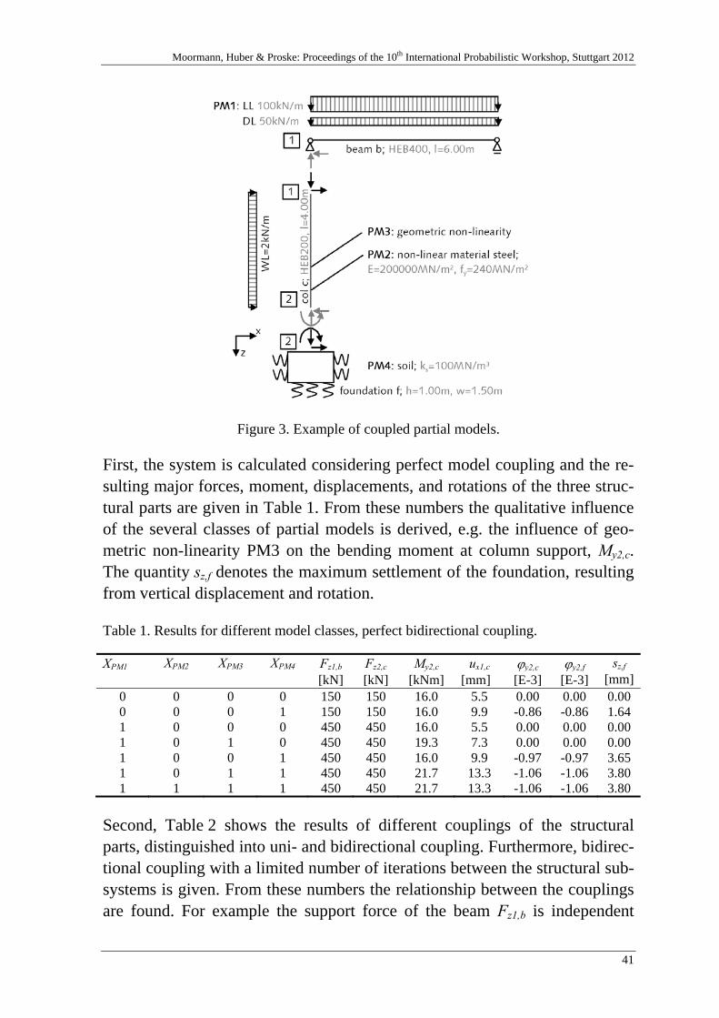
Moormann, Huber & Proske: Proceedings of the 10th International Probabilistic Workshop, Stuttgart 2012
41
Figure 3. Example of coupled partial models.
First, the system is calculated considering perfect model coupling and the re-sulting major forces, moment, displacements, and rotations of the three struc-tural parts are given in Table 1. From these numbers the qualitative influence of the several classes of partial models is derived, e.g. the influence of geo-metric non-linearity PM3 on the bending moment at column support, My2,c. The quantity sz,f denotes the maximum settlement of the foundation, resulting from vertical displacement and rotation.
Table 1. Results for different model classes, perfect bidirectional coupling.
XPM1 XPM2 XPM3 XPM4 Fz1,b Fz2,c My2,c ux1,c ϕy2,c ϕy2,f sz,f
[kN] [kN] [kNm] [mm] [E-3] [E-3] [mm]0 0 0 0 150 150 16.0 5.5 0.00 0.00 0.000 0 0 1 150 150 16.0 9.9 -0.86 -0.86 1.641 0 0 0 450 450 16.0 5.5 0.00 0.00 0.001 0 1 0 450 450 19.3 7.3 0.00 0.00 0.001 0 0 1 450 450 16.0 9.9 -0.97 -0.97 3.651 0 1 1 450 450 21.7 13.3 -1.06 -1.06 3.801 1 1 1 450 450 21.7 13.3 -1.06 -1.06 3.80
Second, Table 2 shows the results of different couplings of the structural parts, distinguished into uni- and bidirectional coupling. Furthermore, bidirec-tional coupling with a limited number of iterations between the structural sub-systems is given. From these numbers the relationship between the couplings are found. For example the support force of the beam Fz1,b is independent
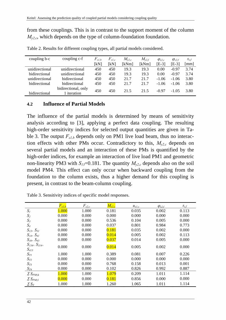
Keitel: Assessing the prediction quality of coupled partial models considering coupling quality
42
from these couplings. This is in contrast to the support moment of the column My2,c, which depends on the type of column-foundation foundation.
Table 2. Results for different coupling types, all partial models considered.
coupling b-c coupling c-f Fz1,b Fz1,c My2,c My2,f ϕy2,c ϕy2,f sz,f
[kN] [kN] [kNm] [kNm] [E-3] [E-3] [mm]unidirectional unidirectional 450 450 19.3 19.3 0.00 -0.97 3.74bidirectional unidirectional 450 450 19.3 19.3 0.00 -0.97 3.74
unidirectional bidirectional 450 450 21.7 21.7 -1.06 -1.06 3.80bidirectional bidirectional 450 450 21.7 21.7 -1.06 -1.06 3.80
bidirectional bidirectional, only
1 iteration 450 450 21.5 21.5 -0.97 -1.05 3.80
4.2 Influence of Partial Models
The influence of the partial models is determined by means of sensitivity analysis according to [3], applying a perfect data coupling. The resulting high-order sensitivity indices for selected output quantities are given in Ta-ble 3. The output Fz1,b depends only on PM1 live load beam, thus no interac-tion effects with other PMs occur. Contradictory to this, My2,c depends on several partial models and an interaction of these PMs is quantified by the high-order indices, for example an interaction of live load PM1 and geometric non-linearity PM3 with S13=0.181. The quantity My2,c depends also on the soil model PM4. This effect can only occur when backward coupling from the foundation to the column exists, thus a higher demand for this coupling is present, in contrast to the beam-column coupling.
Table 3. Sensitivity indices of specific model responses.
Fz1,b Fz2,c My2,c ux1,c ϕy2,f sz,f S1 1.000 1.000 0.181 0.035 0.002 0.113S2 0.000 0.000 0.000 0.000 0.000 0.000S3 0.000 0.000 0.536 0.104 0.005 0.000S4 0.000 0.000 0.037 0.801 0.984 0.773S13= S31 0.000 0.000 0.181 0.035 0.002 0.000S14= S41 0.000 0.000 0.014 0.005 0.002 0.113S34= S43 0.000 0.000 0.037 0.014 0.005 0.000S134= S314= S413 0.000 0.000 0.014 0.005 0.002 0.000 ST1 1.000 1.000 0.389 0.081 0.007 0.226ST2 0.000 0.000 0.000 0.000 0.000 0.000ST3 0.000 0.000 0.768 0.158 0.013 0.001ST4 0.000 0.000 0.102 0.826 0.992 0.887Σ SPM≤k 1.000 1.000 1.079 0.209 1.011 1.114Σ SPM≥l 0.000 0.000 0.181 0.856 0.000 0.000Σ ST 1.000 1.000 1.260 1.065 1.011 1.114
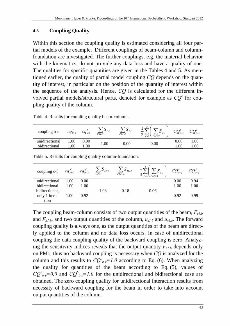
Moormann, Huber & Proske: Proceedings of the 10th International Probabilistic Workshop, Stuttgart 2012
43
4.3 Coupling Quality
Within this section the coupling quality is estimated considering all four par-tial models of the example. Different couplings of beam-column and column-foundation are investigated. The further couplings, e.g. the material behavior with the kinematics, do not provide any data loss and have a quality of one. The qualities for specific quantities are given in the Tables 4 and 5. As men-tioned earlier, the quality of partial model coupling CQ depends on the quan-tity of interest, in particular on the position of the quantity of interest within the sequence of the analysis. Hence, CQ is calculated for the different in-volved partial models/structural parts, denoted for example as CQc for cou-pling quality of the column.
Table 4. Results for coupling quality beam-column.
coupling b-c fFzcq 1 b
uzcq 1 ∑≤ 1.
1PM
FzS ∑≥2
1PM
FzS ∑ ∑= ≥
⎟⎠
⎞⎜⎝
⎛2
1 221
f PMf
Sα bcbCQ − c
cbCQ −
unidirectional 1.00 0.00 1.00 0.00 0.00 0.00 1.00bidirectional 1.00 1.00 1.00 1.00
Table 5. Results for coupling quality column-foundation.
coupling c-f fMycq 2 f
ycq 2ϕ ∑≤ 3.
2PM
MyS ∑≥4
2PM
MyS ∑ ∑= ≥
⎟⎠
⎞⎜⎝
⎛3
1 431
f PMf
Sα cfcCQ − f
fcCQ −
unidirectional 1.00 0.00
1.08 0.18 0.06
0.00 0.94bidirectional 1.00 1.00 1.00 1.00bidirectional, only 1 itera-
tion 1.00 0.92 0.92 0.99
The coupling beam-column consists of two output quantities of the beam, Fz1,b and Fx1,b, and two output quantities of the column, uz1,b and ux1,c. The forward coupling quality is always one, as the output quantities of the beam are direct-ly applied to the column and no data loss occurs. In case of unidirectional coupling the data coupling quality of the backward coupling is zero. Analyz-ing the sensitivity indices reveals that the output quantity Fz1,b depends only on PM1, thus no backward coupling is necessary when CQ is analyzed for the column and this results to CQc
b-c=1.0 according to Eq. (6). When analyzing the quality for quantities of the beam according to Eq. (5), values of CQb
b-c=0.0 and CQbb-c=1.0 for the unidirectional and bidirectional case are
obtained. The zero coupling quality for unidirectional interaction results from necessity of backward coupling for the beam in order to take into account output quantities of the column.
Keitel: Assessing the prediction quality of coupled partial models considering coupling quality
44
The coupling column-foundation consists of three output quantities of the column, Fz2,c, Fx2,c and My2,c, as well as three output quantities of the founda-tion, uz2,f, ux2,f and ϕy2,f. The forward coupling quality is still always one and the backward coupling quality is always zero in case of unidirectional cou-pling. As already mentioned, My2,c depends to some extent on PM4. This is pointed out when comparing the sum of the sensitivity indices of all PM≤3 before and all PM≥4 after the coupling, 1.08 and 0.18. Hence, the coupling quality of the partial models depends on the quality of the forward and back-ward coupling even for response quantities that are after the coupling. The data coupling quality of the support moment is given in Table 5. The resulting coupling qualities are also shown in this Table 5 for two response quantities: first belonging to the column CQc
c-f, which is before coupling and calculated according to Eq. (5), and second for the foundation CQf
c-f, which is after the coupling analyzed according to Eq. (6). The value of CQc
c-f is zero in the uni-directional case, as no information of PM4 can be transferred back to the col-umn. When analyzing CQf
c-f it is observed that a unidirectional coupling still leads to a quality of CQf
c-f=0.94, as the output quantities of the column are mainly defined by the forward coupling and only relatively small parts of the output quantities are influenced by the backward coupling. In case of bidirec-tional coupling with only one iteration between the structure of the column and foundation, a high value of CQf
c-f=0.99 is determined, thus one iteration already gives satisfying results.
4.4 Global Model Quality of the Prediction
Exemplarily, the prediction quality is calculated for the output quantity sup-port moment of the column My2,c and the maximum settlement of the founda-tion sz,f. This example focuses on the effect of coupling type and the consequences from the choice of coupling type. Thus, the quality of the PM1, PM2, and PM3 are chosen not to influence the results and are considered as perfect, MQ=1.0. For PM4 (soil) two different models are considered: a sim-ple approach PM4s with MQPM4s=0.7 and an advanced formulation with MQPM4a=1.0. Apart from the coupling beam-column and column-foundation all other couplings are perfect, CQ=1.0.
The example shall demonstrate the trade-off for choosing a simple soil model, which allows for an iterative bidirectional coupling due to a time-efficient calculation, and an advanced soil formulation only allowing for unidirectional coupling.
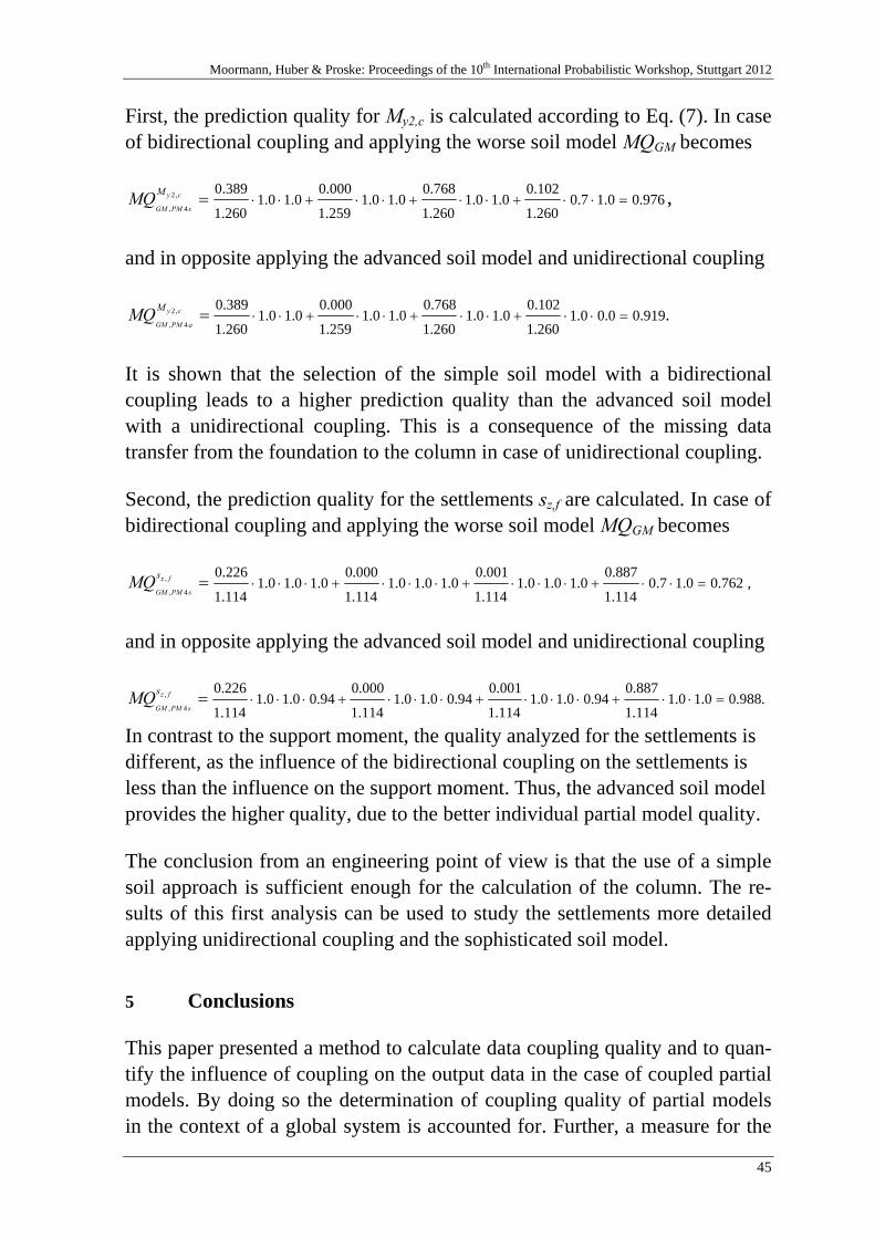
Moormann, Huber & Proske: Proceedings of the 10th International Probabilistic Workshop, Stuttgart 2012
45
First, the prediction quality for My2,c is calculated according to Eq. (7). In case of bidirectional coupling and applying the worse soil model MQGM becomes
976.00.17.0260.1
102.00.10.1
260.1
768.00.10.1
259.1
000.00.10.1
260.1
389.0,2
4,=⋅⋅+⋅⋅+⋅⋅+⋅⋅=cy
sPMGM
MMQ ,
and in opposite applying the advanced soil model and unidirectional coupling
.919.00.00.1260.1
102.00.10.1
260.1
768.00.10.1
259.1
000.00.10.1
260.1
389.0,2
4,=⋅⋅+⋅⋅+⋅⋅+⋅⋅=cy
aPMGM
MMQ
It is shown that the selection of the simple soil model with a bidirectional coupling leads to a higher prediction quality than the advanced soil model with a unidirectional coupling. This is a consequence of the missing data transfer from the foundation to the column in case of unidirectional coupling.
Second, the prediction quality for the settlements sz,f are calculated. In case of bidirectional coupling and applying the worse soil model MQGM becomes
,762.00.17.0114.1
887.00.10.10.1
114.1
001.00.10.10.1
114.1
000.00.10.10.1
114.1
226.0,
4,=⋅⋅+⋅⋅⋅+⋅⋅⋅+⋅⋅⋅=fz
sPMGM
sMQ
and in opposite applying the advanced soil model and unidirectional coupling
.988.00.10.1114.1
887.094.00.10.1
114.1
001.094.00.10.1
114.1
000.094.00.10.1
114.1
226.0,
4,=⋅⋅+⋅⋅⋅+⋅⋅⋅+⋅⋅⋅=fz
sPMGM
sMQ
In contrast to the support moment, the quality analyzed for the settlements is different, as the influence of the bidirectional coupling on the settlements is less than the influence on the support moment. Thus, the advanced soil model provides the higher quality, due to the better individual partial model quality.
The conclusion from an engineering point of view is that the use of a simple soil approach is sufficient enough for the calculation of the column. The re-sults of this first analysis can be used to study the settlements more detailed applying unidirectional coupling and the sophisticated soil model.
5 Conclusions
This paper presented a method to calculate data coupling quality and to quan-tify the influence of coupling on the output data in the case of coupled partial models. By doing so the determination of coupling quality of partial models in the context of a global system is accounted for. Further, a measure for the

Keitel: Assessing the prediction quality of coupled partial models considering coupling quality
46
prediction quality of a global system taking into account coupling quality, in-dividual quality of the partial models, and their influence on the output are taken into account.
The method provides a useful tool to determine the necessity to couple partial models in a uni- or bidirectional manner. Doing so, the algorithm allows for a reduction of complexity of global systems when bidirectional coupling is less important.
Acknowledgements
This research is supported by the German Research Institute (DFG) via Re-search Training Group "Evaluation of Coupled Numerical Partial Models in Structural Engineering (GRK 1462)", which is gratefully acknowledged by the author.
References
[1] Fröbel, T.: Data coupled civil engineering applications: modeling and quality as-sessment methods. Bauhaus-Universität Weimar, Verlag der Bauhaus-Universität Weimar, 2012 - Dissertation
[2] Homma, T.; Saltelli, A.: Importance measures in global sensitivity analysis of non-linear models. Reliability Engineering and System Safety 52 (1996), p. 1-17
[3] Keitel, H.; Karaki, G.; Nikulla, S.; Lahmer, T.; Zabel, V.: Evaluation of coupled par-tial models in structural engineering using graph theory and sensitivity analyses. En-gineering Structures 33 (2011), p. 3726-3736
[4] Lahmer, Z.; Knabe, T.; Nikulla, S.; Reuter, M.: Bewertungsmethoden für Modelle des konstruktiven Ingenieurbaus. Bautechnik Sonderheft 88 (2011), p. 60-64
[5] Most, T.: Assessment of structural simulation models by estimating uncertainties due to model selection and model simplification. Computers and Structures 89 (2011), p. 1664-1672
[6] Saltelli, A.; Ratto, M.; Andres, T.; Campolongo, F.; Cariboni, J.; Gatelli, D.; Saisana, M.; Tarantola, S.: Global sensitivity analysis. The primer. John Wiley and Sons, 2008
[7] Sobol, I.: Sensitivity estimates for nonlinear mathematical models. Mathematical Modeling & Computational Experiment 1 (1993), p. 407-414.
[8] Stein, P.; Lahmer, T.; Bock, S.: Synthese und Analyse von gekoppelten Modellen im konstruktiven Ingenieurbau. Bautechnik Sonderheft 88 (2011), p. 8-11
Moormann, Huber & Proske: Proceedings of the 10th International Probabilistic Workshop, Stuttgart 2012
47
Dependent load combination
T. Poutanen
Department of Civil Engineering, Tampere University of Technology
Tampere, Finland
Abstract: A universal theory on combining loads in structural design is
lacking. Current codes include three methods: dependent, semi-dependent and
independent. These methods are mutually contradicting and inconsistently
applied. The dominant assumption is that loads are combined independently if
the loads are independent, dependently if the loads are dependent and other
loads are combined semi-dependently. However, the permanent loads are
independent but combined always dependently in the current codes contrary to
the basic assumptions. The permanent load and the variable load are combined
sometimes independently and sometimes dependently in the failure state but
always dependently in the serviceability state. Variable loads are combined
usually semi-dependently but sometimes dependently.
This paper explains that the structural loads must always be combined
dependently i.e. the fractile load of the combination load distribution is
obtained by adding up the related fractile loads of the partial load distributions.
The basic reason is that the distributions in the structural design must be the
extreme distributions. Many other arguments are presented, too.
In order to combine variable loads the distributions must be first converted
simultaneous i.e. the loads must be active at the same time. This distribution
alteration induces a combination factor 0.
1 Introduction
The load combination is the key issue in the safety factor and the combination
factor G, Q, M, 0 calculation. The dominant theory is that the loads are
combined independently if the loads are independent, dependently if the loads
are dependent and other loads are combined semi-dependently. However, the
permanent loads are independent but combined always dependently. The
Poutanen: Dependent load combination
48
permanent load and the variable load are combined sometimes independently
and sometimes dependently in the failure state but always dependently in the
serviceability state. Variable loads are combined usually semi-dependently
but sometimes dependently.
An explanation is missing why different combination methods are used. A
uniform theory on the load combination was lacking.
Arguments are presented in this paper that loads must always be combined
dependently. The primary argument is that the combination distribution must
be the extreme distribution. The dependent load combination is universal and
consistent in all cases.
1.1 Current theory
The current load combination theory and its code implementations are
disclosed in references [1, 2, 3, 4, 5, 6, 10, 11].
The basic load combination theory is revealed by MADSEN ET AL [6], MADSEN
[5] and TURKSTRA [11]. Much theoretical research is paid to find out how
variable loads are combined and how the load configuration affects on the
load combination. The current variable load combination is based on
Turkstra’s method TURKSTRA [11]: The combination load is the higher load
which is obtained when one load is constant and the other load has a random
value. In this load combination, the load configuration has no effect.
The theoretical references [5, 6, 11] and references [1, 2, 3, 4, 10, 11]
explaining the actual load combination in the code, describe that the loads are
stochastic and combined independently. However, this concept is not
consistently applied. No reference explains why permanent loads are
combined dependently although these loads are independent?
If there are many loads, e.g. imposed loads of a multi storey house1 or many
permanent loads, the independent load combination results in an unrealistic
outcome as the reliability vanishes. The current load combination theory does
not address this contradiction either.
The references [1, 2, 3, 4, 5, 6, 10, 11] do not address several other significant
issues of the load combination:
1 The unrealistic outcome of the independent load combination is recognized in an Eurocode background
document: Imposed loads on floors and roofs (1990) “The storey-dependent reduction formulas of the code-
draft are not scientifically derived…”.
Moormann, Huber & Proske: Proceedings of the 10th International Probabilistic Workshop, Stuttgart 2012
49
The extreme function, i.e. the rule of the maximum load combination.
The correlation of the loads due to the equality design equation.
The correlation of the loads when the loads are proportions of another load.
The load losing and the uneven failure probability of the independent combination.
The independent combination contradicts the linearity and Hook’s law.
1.2 Dependent, semi-dependent and independent load combination
Two loads are combined dependently by adding up the distributions by
fractiles i.e. a load X with an item xi in fractile i and a load Y with an item yi in
the same fractile i are combined dependently to obtain the combination load
XY with an item xyi in fractile i by adding up xi and yi, i.e. xyi = xi + yi,
POUTANEN [7, 8]. If the Monte Carlo simulation is used to combine the loads,
in the dependent combination one seed number is used. The same
combination load is obtained when several random load pairs xi , yi are
generated and the combination load distribution is constructed from these load
pairs considering the extreme function i.e. the maximum load rule. If the
convolution equation is used to combine the loads, the deviation of the
combination load is fixed in a way the combination distribution crosses the
crossing point of the partial distributions POUTANEN [7, 8]. In the dependent
combination, the action of a new load in the combination is independent of
other loads in the load combination. When the loads are combined
dependently in the actual structural design, the design values of the partial
loads are added up as such without any reductions, combination factors etc.
and without any load losing.
The semi-dependent combination is an imprecise abstraction. Several semi-
dependent combination methods exist, e.g. Turkstra’s method, TURKSTRA
[11], where one load has a constant value and the other load has a random
value. The semi-dependent combination should lie between the dependent and
independent combination. This is normally true at least at high fractiles1. In
the current codes the semi-dependent combination is carried out by Turkstra’s
load combination model TURKSTRA [11] to combine variable loads. In the
actual code two loads are added up with a combination factor 0 in the lesser
load. Turkstra’s load combination model is approximate. This combination is
1 Turkstra’s combination load depends on how the constant value is defined. It is normally the mean value
(or approximately the mean value) when Tukstra’s combination is less than the independent combination
load and also less that the dependent combination load (as the dependent combination load is the highest
one).
Poutanen: Dependent load combination
50
a discontinuous1 function of partial loads and it does not include two relevant
concepts in the load combination: the load duration and the simultaneity.
Turkstra’s load combination includes a load losing.
In the independent combination, the loads are combined randomly e.g. by
using the convolution equation or by using Ferry Borges – Castanheta’s
method, ISO 2394 [4], or by using the Monte Carlo simulation and two seed
numbers without the extreme function i.e. the maximum load combination
rule. In the independent combination, the action of the new combination load
depends on the earlier loads in the combination2. The independent
combination is often applied in the combination of the permanent and the
variable load and to define the material safety factor M. A part of the load, ca
0...10 %, vanishes in this combination and therefore the safety factor M
includes a reduction factor of ca 0.9...1.
In the semi-dependent and in the independent combinations, each new load in
the combination decreases the total safety factor. If the number of loads is
infinite, there is no safety and the total load is the sum of the mean partial
loads.
The current terms dependent and independent combination are misleading as
in the independent combination the partial loads may be independent or
dependent but the combination load is dependent of the partial loads and in
the dependent combination vice versa. Therefore it would be clearer to use
other terms. The independent combination may be called “indefinite” or
“random” summation. Correspondingly, the dependent combination may be
called “definite” or “accumulation” summation.
1.3 Load combination in current codes
Loads are combined in the current codes in three ways:
Permanent loads are always combined dependently.
A permanent and a variable load are combined in the failure state
sometimes dependently and sometimes independently but in the
serviceability state always dependently.
1 The actual load is the function of the load ratio F( ), it is continuous but its derivative dF( )/d is
discontinuous.
2 This is a clear argument that the independent load combination is wrong. It is impossible, for instance, that
the effect of the snow load on a roof would depend on the permanent load of the roof and the effect was
different on a light and a heavy roof.
Moormann, Huber & Proske: Proceedings of the 10th International Probabilistic Workshop, Stuttgart 2012
51
Two variable loads are always combined semi-dependently if these
loads are the first and the second variable load in the load combination,
but always dependently if the loads are third, fourth etc. load in the load
combination.
EUROCODE [1] includes three options to combine the permanent and the
variable load, 6.10, 6.10a,b and 6.10a,mod. The first one is dependent and the
others are independent. Finnish Eurocode is based on 6.10a,mod.
1.4 Contradictions in current codes
The basis of the current load combination theory is questionable as three
contradicting combination methods exist and these methods are applied
inconsistently:
The permanent G and the variable Q load are usually considered
independent but they are independent only during one year and
virtually fully correlated and dependent during the service time of a
structure, 50 years1.
Permanent loads are independent and according to the current load
combination hypotheses, these loads should be combined
independently but they are always combined dependently. Permanent
loads cannot be combined independently as the outcome was
unrealistic.
Eurocode includes three load combination rules 6.10, 6.10a,b and
6.10a,mod. The first one is dependent, and the others independent. The
code writer cannot give a clear directive about the load combination.
In the current codes, permanent and variable loads are combined in the
failure state sometimes dependently and sometimes independently but
in the serviceability state always dependently. It is evident that the
loads must be combined consistently in the same way in all cases.
Variable loads are combined semi-dependently if the loads are the first
and the second load in the load combination but thereafter the loads are
combined always dependently.
1 All Q-load values below fractile 0.98 occur during 50 years. Whichever the G-load is below the fractile
0.98 there is a Q-load at the same fractile.
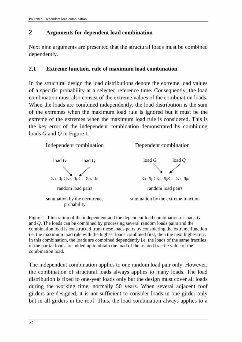
Poutanen: Dependent load combination
52
2 Arguments for dependent load combination
Next nine arguments are presented that the structural loads must be combined
dependently.
2.1 Extreme function, rule of maximum load combination
In the structural design the load distributions denote the extreme load values
of a specific probability at a selected reference time. Consequently, the load
combination must also consist of the extreme values of the combination loads.
When the loads are combined independently, the load distribution is the sum
of the extremes when the maximum load rule is ignored but it must be the
extreme of the extremes when the maximum load rule is considered. This is
the key error of the independent combination demonstrated by combining
loads G and Q in Figure 1.
Figure 1. Illustration of the independent and the dependent load combination of loads G
and Q. The loads can be combined by processing several random loads pairs and the
combination load is constructed from these loads pairs by considering the extreme function
i.e. the maximum load rule with the highest loads combined first, then the next highest etc.
In this combination, the loads are combined dependently i.e. the loads of the same fractiles
of the partial loads are added up to obtain the load of the related fractile value of the
combination load.
The independent combination applies to one random load pair only. However,
the combination of structural loads always applies to many loads. The load
distribution is fixed to one-year loads only but the design must cover all loads
during the working time, normally 50 years. When several adjacent roof
girders are designed, it is not sufficient to consider loads in one girder only
but in all girders in the roof. Thus, the load combination always applies to a
load G load Q load G load Q
Dependent combination
gi1, qj1; gi2, qj2;… gin, qjn
random load pairs
summation by the extreme function
Independent combination
gi1, qj1; gi2, qj2;… gin, qjn
random load pairs
summation by the occurrence
probability
Moormann, Huber & Proske: Proceedings of the 10th International Probabilistic Workshop, Stuttgart 2012
53
group of loads, thus the maximum load combination and the dependent
combination must be employed.
2.2 Common sense reasoning
The dependent combination can be deduced by common sense reasoning:
Assume a material (or a structure) has the survival probability S and the
resistance 1 for the permanent load G alone and the variable load Q load
alone. Now, if the material is loaded by 0.5G and 0.5Q and the loads are
combined independently, the material has the resistance of ca 1.11 and if
combined dependently, it is 1. The independent combination is unrealistic. It
is impossible that the effect of one load decreases if the other load is present.
The reason for the high resistance, if the loads are combined independently, is
the load losing.
2.3 Equality equation
The basic design equation of the structural design with the permanent load G,
the variable load Q and the material property M is
(1)
If we apply an equality equation, a definite dependence and correlation exists
between the distributions G, Q as the material property M is constant
regarding the loads. G and Q have a full negative correlation. When one load
is increased the other decreases correspondingly. Due to this correlation the
loads G and Q must be combined dependently regardless of whether they are
independent or dependent otherwise.
2.4 Linearity, Hook’s law
Hook’s law directs one basic rule in the structural design, linearity: when a
load has a certain effect at one load level, the same effect occurs by the same
load at any other load level. The independent load combination is in contrast
with the Hook’s law and the linearity:
One realization of the independent load combination is the combination rule
6.10a,mod of Eurocode. In this load combination with low permanent load
when the variable load increases no effect occurs.
1 In Eurocode more precisely 1.0646, VG,normal = 0.09147, VQ,gumbel = 0.4, = 3.826, combination rule 6.10.
G G Q QM
M
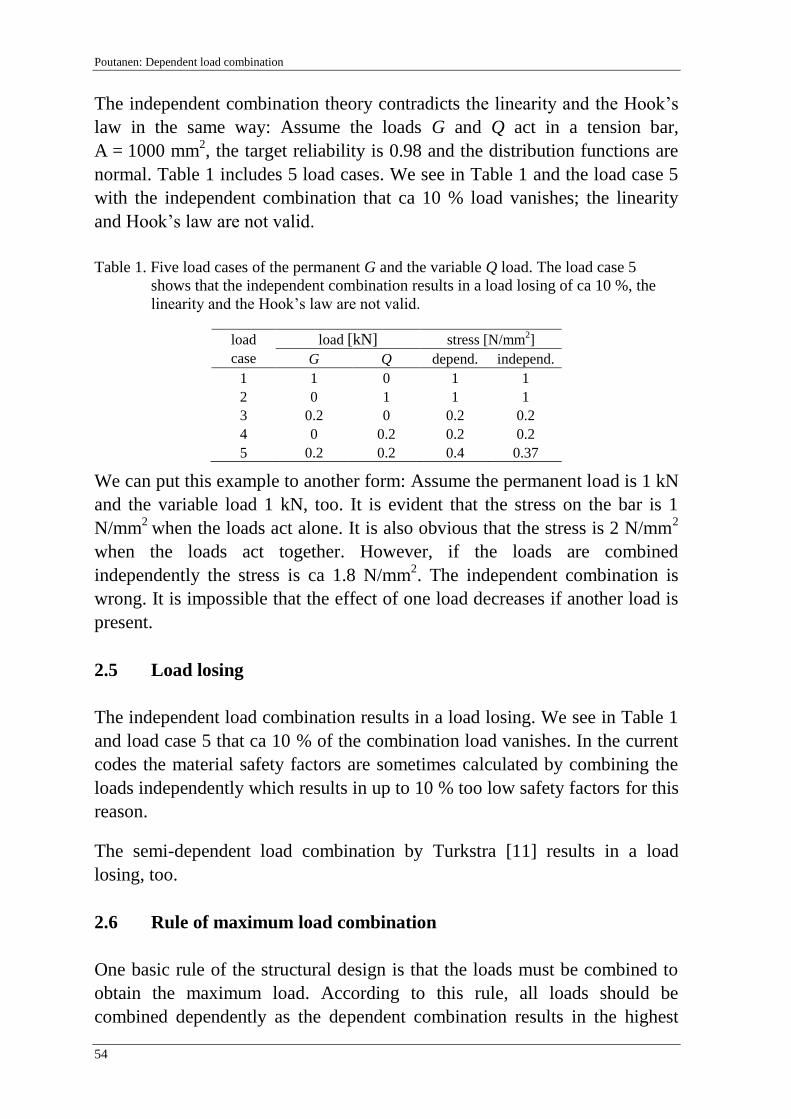
Poutanen: Dependent load combination
54
The independent combination theory contradicts the linearity and the Hook’s
law in the same way: Assume the loads G and Q act in a tension bar,
A = 1000 mm2, the target reliability is 0.98 and the distribution functions are
normal. Table 1 includes 5 load cases. We see in Table 1 and the load case 5
with the independent combination that ca 10 % load vanishes; the linearity
and Hook’s law are not valid.
Table 1. Five load cases of the permanent G and the variable Q load. The load case 5
shows that the independent combination results in a load losing of ca 10 %, the
linearity and the Hook’s law are not valid.
load
case
load [kN] stress [N/mm2]
G Q depend. independ.
1 1 0 1 1
2 0 1 1 1
3 0.2 0 0.2 0.2
4 0 0.2 0.2 0.2
5 0.2 0.2 0.4 0.37
We can put this example to another form: Assume the permanent load is 1 kN
and the variable load 1 kN, too. It is evident that the stress on the bar is 1
N/mm2
when the loads act alone. It is also obvious that the stress is 2 N/mm2
when the loads act together. However, if the loads are combined
independently the stress is ca 1.8 N/mm2. The independent combination is
wrong. It is impossible that the effect of one load decreases if another load is
present.
2.5 Load losing
The independent load combination results in a load losing. We see in Table 1
and load case 5 that ca 10 % of the combination load vanishes. In the current
codes the material safety factors are sometimes calculated by combining the
loads independently which results in up to 10 % too low safety factors for this
reason.
The semi-dependent load combination by Turkstra [11] results in a load
losing, too.
2.6 Rule of maximum load combination
One basic rule of the structural design is that the loads must be combined to
obtain the maximum load. According to this rule, all loads should be
combined dependently as the dependent combination results in the highest

Moormann, Huber & Proske: Proceedings of the 10th International Probabilistic Workshop, Stuttgart 2012
55
load. This rule is valid and must always be obeyed. In the current theory, this
rule is sometimes ignored as the independent loads are wrongly considered
demanding the independent load combination.
2.7 Imposed loads
Imposed loads on the floors of a multi storey house are different from other
loads as they are proportions of another load, the total imposed load in the
house. Therefore the imposed loads on the floors are correlated and must be
combined dependently.
2.8 Permanent loads
Permanent loads are independent but combined in all codes always
dependently i.e. correctly contrary to the current load combination theory.
Permanent loads cannot be combined independently as the result was
unrealistic. The safety would vanish in case of many loads.
2.9 Many loads
If loads are combined independently or semi-dependently, each new load in
the combination decreases the total safety. In case of many loads, e.g.
permanent or imposed loads of a multi storey house, the safety vanishes,
which is unrealistic.
3 Combination of variable loads
The combination of variable loads A and B is like the combination of the
permanent and the variable loads G and Q, POUTANEN [9]. The distribution of
one load is converted to the active time of this load when it becomes
analogous to the permanent load. The distribution conversion induces a
combination factor 0. This load and the other variable load are combined
dependently without any further combination factors or reductions which
would induce a load losing. The loads A and B may have different active
times; therefore each load must be converted in turn to its active time and the
greater load combination is selected.
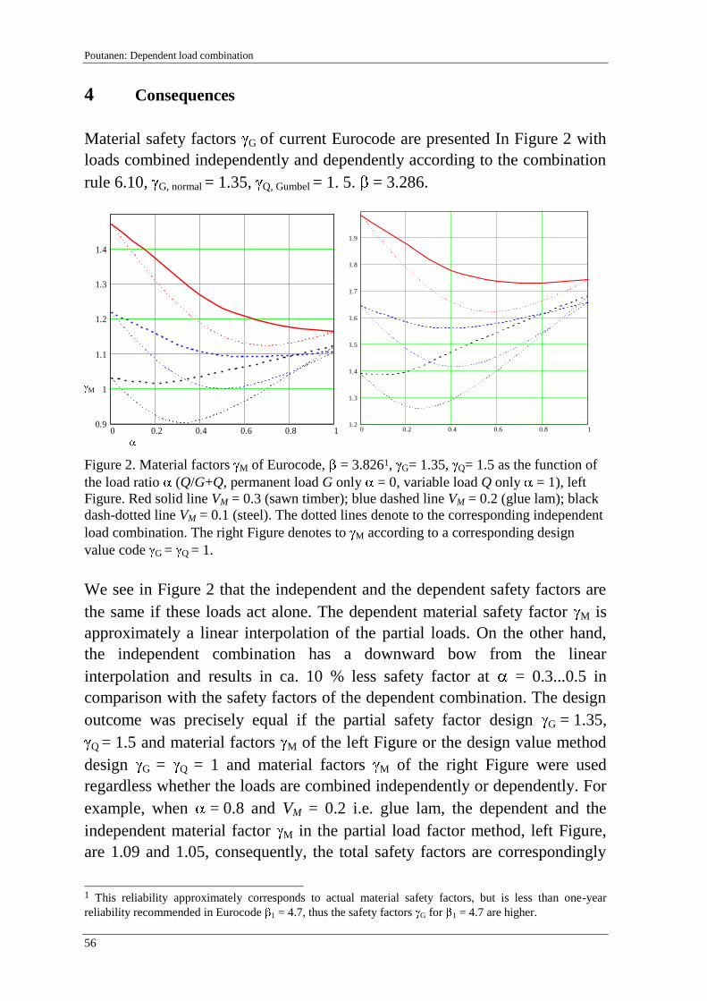
Poutanen: Dependent load combination
56
4 Consequences
Material safety factors G of current Eurocode are presented In Figure 2 with
loads combined independently and dependently according to the combination
rule 6.10, G, normal = 1.35, Q, Gumbel = 1. 5. = 3.286.
Figure 2. Material factors M of Eurocode, = 3.8261, G= 1.35, Q= 1.5 as the function of
the load ratio (Q/G+Q, permanent load G only = 0, variable load Q only = 1), left
Figure. Red solid line VM = 0.3 (sawn timber); blue dashed line VM = 0.2 (glue lam); black
dash-dotted line VM = 0.1 (steel). The dotted lines denote to the corresponding independent
load combination. The right Figure denotes to M according to a corresponding design
value code G = Q = 1.
We see in Figure 2 that the independent and the dependent safety factors are
the same if these loads act alone. The dependent material safety factor M is
approximately a linear interpolation of the partial loads. On the other hand,
the independent combination has a downward bow from the linear
interpolation and results in ca. 10 % less safety factor at = 0.3...0.5 in
comparison with the safety factors of the dependent combination. The design
outcome was precisely equal if the partial safety factor design G = 1.35,
Q = 1.5 and material factors M of the left Figure or the design value method
design G = Q = 1 and material factors M of the right Figure were used
regardless whether the loads are combined independently or dependently. For
example, when = 0.8 and VM = 0.2 i.e. glue lam, the dependent and the
independent material factor M in the partial load factor method, left Figure,
are 1.09 and 1.05, consequently, the total safety factors are correspondingly
1 This reliability approximately corresponds to actual material safety factors, but is less than one-year
reliability recommended in Eurocode 1 = 4.7, thus the safety factors G for 1 = 4.7 are higher.
0 0.2 0.4 0.6 0.8 10.9
1
1.1
1.2
1.3
1.4
1.5
.9
eueo0430
eueoNI0430
eueo0420
eueoNI0420
eueo0410
eueoNI0410
10
100
0 0.2 0.4 0.6 0.8 11.2
1.3
1.4
1.5
1.6
1.7
1.8
1.9
2
1.2
US0430a
US0430NIa
US0420a
US0420NIa
US0410a
US0410NIa
10
100
M

Moormann, Huber & Proske: Proceedings of the 10th International Probabilistic Workshop, Stuttgart 2012
57
GQ1.
M, 1.62 and 1.54 which are equal to the total safety factors of the design
value method, right Figure. However, in the actual design minor variations
occur as the current codes do not include the concrete material safety factors
M but these factors are approximated but constants i.e. the curved and
inclined lines are horizontal lines.
The dependent load combination in the actual design are summarized as
follows:
The combination rules including two permanent load factors e.g. the rules 6.10a,b
and 6.10a,mod of Eurocode are induced from the independent load combination
and these combination rules should be deleted.
The total safety factor calculated from G and Q loads t = ( G, Q, M) is up to
10 % too low, if the permanent and the variable load is combined independently.
The safety factors of the current codes are normally higher than the target safety
factors and the actual error is less. However, in some cases this error has its full
effect.
Two variable loads are currently combined semi-dependently, which results in up to
ca 30 % too low combination factors 0 POUTANEN [9].
The combination factor 0 for the snow load is currently 0.5...0.7 but should be
adjusted according to the duration of the snow load: one week 0 ≈ 0.75; one moth
0 ≈ 0.85 and two moths, 0 ≈ 0.90. As this factor is close to unity a feasible
approximation is to set it at unity, 0 = 1.
The combination factor 0 of a short duration load e.g. imposed load and wind load
combined with each other or with snow (except imposed load – imposed load)
depends on the duration of the load: one minute, 0 ≈ 0.55; 10 minutes, 0 ≈ 0.6;
ten hours, 0 ≈ 0.65; one day, 0 ≈ 0.7 and one week, 0 ≈ 0.75, POUTANEN [9].
The current imposed load factor is 0 = 0.7 but it should be 1. The reason is that the
imposed loads on floors are dependent and proportions of the whole imposed load
of the house2.
The unsafe error of the reliability model due to the independent and the semi-
dependent load combination is up to ca 15 % in two loads and up to ca 20 % in
three loads. The unsafe error of the actual code is less, up to ca 15 %, as the safety
factors are often selected higher than obtained from the independent and semi-
dependant calculation.
The dependent combination affects on the safety and the combination factors
only, not the design equations and the design processes.
1 GQ = 0.2.1.35 + 0.8
.1.5 = 1.470
2 The characteristic imposed loads in current codes are high enough to compensate the 0 error.
Poutanen: Dependent load combination
58
The dependent load combination results in a partial safety factor code with
one permanent load factor e.g. combination rule 6.10 of Eurocode or a unity
load factor code G = Q = 1. A partial safety factor code including one
permanent load factor can always be converted in a unity load factor code
G = Q = 1 with an equal reliability and equal design outcome. This change
does not affect the current limit state design concept. Thus the option
G = Q = 1 is attractive as it simplifies the code and decreases the calculation
work. If we set G = Q = 1 with M semi-variable in variable G-Q-loads
(constant in normal load cases), such code has far better reliability accuracy
with less calculation work than any current code, G ≠ Q ≠ 1, constant M.
5 Conclusions
Structural loads must be combined dependently. It is the consistent and the
universal load combination in all cases:
The permanent loads with each other G – G and the permanent load and the
variable load G – Q are combined dependently as such i.e. without combination or
reduction factors which would induce a load losing.
The variable loads Q – Q are combined dependently, too after the distributions are
altered in a way the loads are simultaneous i.e. they are active with each other at the
same time. The distribution alteration induces a combination factor 0.
If variable loads are proportions of another load (e.g. imposed loads of a multi
storey house), they are combined dependently i.e. without a combination factor,
0 = 1.
The maximum load combination rule, the equality equation, Hook’s law, the
linearity and the load losing demand the dependent load combination.
A good option is to set G = Q = 1 and semi-variable M. This setting results in
much better reliability accuracy than in current codes with less calculation work
and simpler code.
The current terms dependent and independent combination are misleading. It would
be clearer to use terms “accumulation” or “definite” summation and “random” or
“indefinite” summation.
The accumulation summation of loads is reliable, it is simple and the required
design work is little.

Moormann, Huber & Proske: Proceedings of the 10th International Probabilistic Workshop, Stuttgart 2012
59
Acknowledgement
When writing this paper I have got valuable comments from Professor Keijo Ruohonen, Tampere University of Technology.
References
[1] CodeCal, A soft ware for reliability calculation, 2002, http://www.jcss.ethz.ch
[2] EN 1990:2002 Eurocode – Basis of structural design, European Committee for
standardization, Bruxelles
[3] Gulvanessian H., Calgaro J-A., Holicky M., Designer’s Guide to EN 1990,
EUROCODE: Basis of structural design, Thomas Telford Publishing, London, 2002
[4] ISO 2394, General principles on reliability for structures, International Organization
for Standardization, Geneva, Switzerland, 1996
[5] Madsen H., O., Load Models and Load Combination, Technical University of
Denmark, Rapport nr R 113, 1979
[6] Madsen H., O., Krenk S., Lind N., C., Methods of Structural Safety, Prentice-Hall
Inc. NJ, USA, 1986
[7] Poutanen T., Safety factors and design codes, Joint IABSE – fib Conference,
Dubrovnik, May 3-5, 2010
[8] Poutanen T., Calculation of partial safety factors, Applications of Statistics and
Probability in Civil Engineering – Faber, Köhler & Nishijima (eds), Taylor &
Francis Group, London, 2011
[9] Poutanen T., Combination factors 0 in structural design, A journal article submitted
for review, 2011
[10] Probabilistic Model Code, Part 1, Basis of Design, http://www.jcss.ethz.ch
[11] Turkstra C., J., Theory of Structural Safety, SM Study No. 2, Solid Mechanics
Division, University of Waterloo, Waterloo, Ontario, 1970

Poutanen: Dependent load combination
60
Moormann, Huber & Proske: Proceedings of the 10th International Probabilistic Workshop, Stuttgart 2012
61
Reliability-based design optimization
of damage-tolerant elastoplastic frames
Dimos C. Charmpis
Department of Civil and Environmental Engineering, University of Cyprus,
75 Kallipoleos Str., P.O. Box 20537, 1678 Nicosia, Cyprus
Abstract: This work is concerned with the explicit treatment of progressive
collapse resistance within the process of structural design optimization under
uncertainty. Progressive collapse resistance is associated with the damage tol-
erance of a structural system and controls the ability of the system to sustain
local damage (e.g. loss of a structural component) by minimizing the potential
of triggering system failure (progressive partial/full collapse). The present
work focuses on the reliability-based optimum design of damage-tolerant elas-
toplastic steel frames with correlated random member properties. For this pur-
pose, additional reliability constraints concerning the structure with artificial
local damage are incorporated into the Reliability-Based Design Optimization
(RBDO) formulation, which –in its classical form– takes only one reliability
constraint associated with the intact (non-damaged) structure into account and
aims in minimizing structural cost (or material volume/weight). The direct
Monte Carlo simulation procedure is employed to perform structural reliability
analyses, while a specialized heuristic random number generator is used to
sample from multivariate probability distributions with their marginals being
the distributions of the arbitrarily distributed and intercorrelated random mem-
ber properties. The resulting RBDO approach, which is implemented using a
discrete Simulated Annealing optimizer, is capable of producing cost-effective
designs for elastoplastic frames with acceptable system damage tolerance.
1 Introduction
Reliability-Based Design Optimization (RBDO) is the most common ap-
proach applied to structural design optimization problems taking into account
uncertainties in material properties, geometric parameters, loads etc. The op-
timization process aims in detecting the optimum design by minimizing the
weight or cost of a structure subject to constraints ensuring adequate perfor-
mance for the structural members and/or the overall system. In RBDO, typi-
cally one structural reliability constraint is incorporated by pre-specifying the
D.C. Charmpis: Reliability-based design optimization of damage-tolerant elastoplastic frames
62
maximum allowable failure probability of the structure for the finally
achieved design.
The present work is concerned with the reliability-based optimum design of
elastoplastic steel frames, which consist of members with correlated random
structural properties. In the framework of the implemented RBDO process,
the reliability constraint is imposed by adopting a maximum allowable col-
lapse probability of the elastoplastic frame designed.
In addition to the above reliability constraint focusing on the system re-
sistance of an intact (non-damaged) frame, additional probabilistic design re-
quirements on the system resistance of the frame suffering artificial local
damage are considered. The term ‘artificial local damage’ is used to refer to a
scenario of local structural failure, which may trigger progressive collapse of
the structure. Insensitivity to such local failures is an important property of
the structure, which can be considered during the design process. In this work,
additional constraints are included in the RBDO procedure, in order to control
the reliability (i.e. the non-collapse probability) of the structure under any as-
sumed damage scenario(s). A method based on the notional removal of key-
members of a frame is used to define local damage scenarios in an effort to
direct the optimizer towards identifying a structural design, which provides
adequate alternate load paths (and therefore sufficient structural reliability)
when local failure occurs in the structure.
Structural reliability analyses are conducted in this paper with the direct Mon-
te Carlo (MC) simulation procedure combined with the Response Surface
method. A specialized random number generation procedure is utilized to
handle the task of sampling from a multivariate probability distribution with
arbitrarily distributed and intercorrelated marginals, in order to obtain the
random realizations required to perform MC simulations. A discrete Simulat-
ed Annealing (SA) optimizer is employed to handle the RBDO problem for
the steel frames considered. The numerical results obtained for a test example
demonstrate the effectiveness and significance of the proposed optimization
approach.
2 Structural reliability analysis
This section describes the approach employed in the present work to conduct
structural reliability analysis, i.e. to estimate the probability of partial/full col-
lapse (failure probability) of an elastoplastic steel frame.
Moormann, Huber & Proske: Proceedings of the 10th International Probabilistic Workshop, Stuttgart 2012
63
2.1 Direct Monte Carlo (MC) simulation
The direct MC simulation method, which is utilized in this paper, is the most
well-known approach for handling structural reliability problems [6]. Based
on samples simulated following the joint probability density function of the
random variables of the problem at hand, the failure probability is simply es-
timated as the expectation of an indicator function denoting structural failure
or non-failure. Direct MC simulation is a general method that is applicable to
any structural problem, for which a deterministic solver can be invoked, in
order to determine output samples for the response quantities of interest by
performing a deterministic structural analysis for each MC simulation.
The convergence rate of the MC simulation procedure is independent of the
number of random variables considered, their distribution functions and their
intercorrelations. Therefore, this procedure seems to be suitable for reliability
calculations with several arbitrarily distributed and intercorrelated random
variables, as is the case in the present work. On the other hand, the conver-
gence rate depends on the value of the failure probability to be calculated and
the number of simulations to be performed. As a consequence, low failure
probabilities can be estimated with acceptable accuracy only by conducting
rather large numbers of simulations, which is a computationally very demand-
ing task, especially when it has to be repeatedly executed in the framework of
the RBDO process.
In order to alleviate the aforementioned high computational workload, deter-
ministic structural analysis results are approximated by employing the Re-
sponse Surface (RS) method. The deterministic solver utilized in this paper
calculates the collapse load factor of the structure under consideration by exe-
cuting a limit elastoplastic frame analysis [15]. Hence, using this solver, a
small number of deterministic limit elastoplastic analyses are conducted for
the structure, in order to produce data points for the regression calculations
required to determine unknown coefficients involved in the RS function.
Then, the collapse load factor of the structure is conveniently and inexpen-
sively estimated at each MC simulation by evaluating a simple RS expression
instead of performing a time consuming limit elastoplastic frame analysis.
2.2 Multivariate Random Number Generation (RNG)
For the elastoplastic steel frames considered in the present work, correlations
are assumed among random yield strengths at different structural components.
These statistical dependences among material properties of different steel
members depend on the way these members are constructed at site or manu-
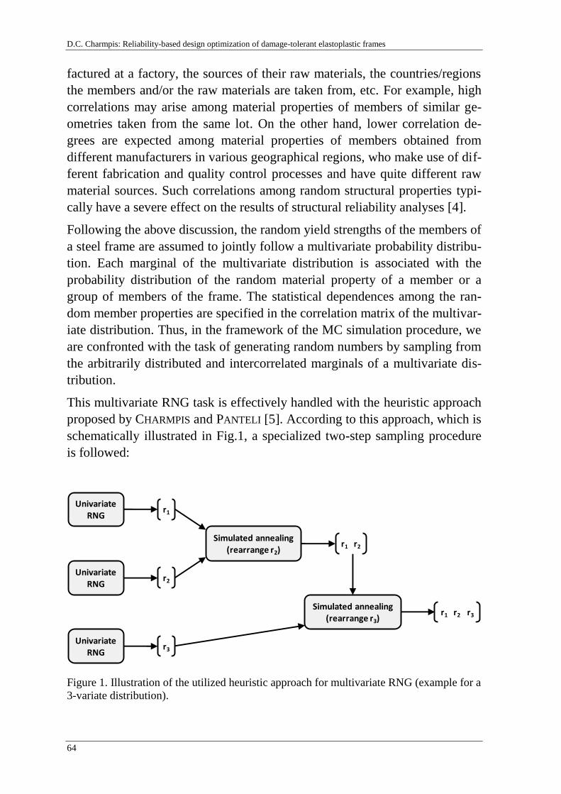
D.C. Charmpis: Reliability-based design optimization of damage-tolerant elastoplastic frames
64
factured at a factory, the sources of their raw materials, the countries/regions
the members and/or the raw materials are taken from, etc. For example, high
correlations may arise among material properties of members of similar ge-
ometries taken from the same lot. On the other hand, lower correlation de-
grees are expected among material properties of members obtained from
different manufacturers in various geographical regions, who make use of dif-
ferent fabrication and quality control processes and have quite different raw
material sources. Such correlations among random structural properties typi-
cally have a severe effect on the results of structural reliability analyses [4].
Following the above discussion, the random yield strengths of the members of
a steel frame are assumed to jointly follow a multivariate probability distribu-
tion. Each marginal of the multivariate distribution is associated with the
probability distribution of the random material property of a member or a
group of members of the frame. The statistical dependences among the ran-
dom member properties are specified in the correlation matrix of the multivar-
iate distribution. Thus, in the framework of the MC simulation procedure, we
are confronted with the task of generating random numbers by sampling from
the arbitrarily distributed and intercorrelated marginals of a multivariate dis-
tribution.
This multivariate RNG task is effectively handled with the heuristic approach
proposed by CHARMPIS and PANTELI [5]. According to this approach, which is
schematically illustrated in Fig.1, a specialized two-step sampling procedure
is followed:
UnivariateRNG
UnivariateRNG
UnivariateRNG
Simulated annealing(rearrange r2)
Simulated annealing(rearrange r3)
r1
r2
r3
r1 r2
r1 r2 r3
Figure 1. Illustration of the utilized heuristic approach for multivariate RNG (example for a
3-variate distribution).
Moormann, Huber & Proske: Proceedings of the 10th International Probabilistic Workshop, Stuttgart 2012
65
1. First a univariate random sample is independently generated from each
specified member property’s distribution (i.e. from each marginal prob-
ability distribution) – e.g. see the generated univariate random samples
r1,r2,r3 in Fig. 1. Any specified statistical dependences are not taken in-
to account yet, therefore zero-correlations are typically obtained among
the marginals of the multivariate random sample produced in this first
step.
2. The univariate random samples of the first step are appropriately rear-
ranged by a discrete Simulated Annealing (SA) optimization algorithm,
in order to induce the desired correlations among the marginals of the
generated multivariate sample – e.g. see the finally obtained correlated
multivariate random sample [r1 r2 r3] in Fig. 1. The SA optimizer is
invoked to rearrange the generated univariate samples one after the
other (only the first univariate sample r1 is left unchanged): the margin-
al sample ri is rearranged to become appropriately correlated with
r1,r2,...,ri-1 before processing the next sample (ri+1). The random num-
bers generated for the univariate samples in the first step are not altered
by the SA procedure, only the positions of these numbers within each
univariate sample vector are changed until reaching the required corre-
lation structure. The correlation accuracy attained is monitored through
the objective function minimized by the SA algorithm, which is an er-
ror index measuring the difference between the target and achieved cor-
relations.
The above multivariate RNG procedure is distribution-free, as it allows us to
handle actually any type of marginal distribution, for which a corresponding
univariate random number generator is available. Moreover, the SA optimizer
can induce any values and patterns of target correlations. The details of this
generally applicable heuristic multivariate RNG approach can be found in [5].
3 Gaining progressive collapse resistance through alternate load
paths
Treating the progressive collapse resistance of a structure during the design
phase is generally not a straightforward task. Although the importance of this
task is recognized by many design engineers and there are already design
guidelines (e.g. [8,7]) and even codes (e.g. [12]) that include provi-
sions/requirements associated with progressive collapse resistance, it is not
clear how to enhance the quality of structural designs, in order to achieve im-
proved tolerance against local damage.
D.C. Charmpis: Reliability-based design optimization of damage-tolerant elastoplastic frames
66
The requirement for progressive collapse resistance is handled in the present
work by applying the alternate path method. According to this method, the
designer aims in specifying a structural design that, in the event of local fail-
ure (e.g. loss of certain columns and/or beams of a building), allows the redis-
tribution of the loads acting on the damaged structure, in order to be safely
transferred to the ground through alternate load paths employing the remain-
ing undamaged members. In order to achieve such structural designs, the de-
signer can consider an artificial local failure caused by the notional removal
of certain column(s) [8,7]. The response of the artificially damaged structure
may then be assessed, in order to determine the remaining structural re-
sistance capabilities of the structure, which is required to be able to withstand
certain actions that may arise after the occurrence of local damage.
In order to enhance the collapse resistance of the artificially damaged struc-
ture, its structural members need to be adequately strengthened, because they
will have to carry additional loads in the event of column(s) loss. A straight-
forward implementation of the alternate path method is to create a ‘bridge’
over the damaged region by strengthening respective beams (over the dam-
aged region) and columns (beside and below the damaged region). Then, an
obvious disadvantage of this approach is that it results in a local type of
strengthening, since it is directly linked to a particular failure scenario. Clear-
ly, in the event of a column loss at a storey-level that is higher than that of the
‘bridge’ formed, the bridge will practically have no effect on the collapse re-
sistance of the structure given the particular local failure.
The aim of the present work is to investigate the application of the alternate
path method in a way that progressive collapse requirements are satisfied with
minimum additional cost. Through the proposed RBDO implementation it is
possible to ‘discover’ how to meet such requirements in an optimal way by
learning from optimization results.
4 Reliability-Based Design Optimization (RBDO)
Structural design optimization is typically formulated as a single-objective
optimization task aiming at the minimization of the cost (or material vol-
ume/weight) of the structure considered. In RBDO, structural reliability (i.e.
failure probability) is explicitly taken into account through a related con-
straint. The RBDO formulation considered in the present work is as follows:
minimize C(d)
subject to Pf (d) ≤ Pf,max
Moormann, Huber & Proske: Proceedings of the 10th International Probabilistic Workshop, Stuttgart 2012
67
di D, i=1,…,nd (1)
In the above formulation, d is the vector of design variables di (i=1,2,…,nd),
which may take values only from a given set D representing the available de-
sign options (D is often referred to as the ‘design space’), while C(d) denotes
the objective function to be minimized (i.e. the structural cost or material vol-
ume/weight). Pf (d) is the structural failure probability expressed as a function
of the design variables and Pf,max is the maximum allowable failure probabil-
ity. Thus, RBDO aims in gaining control over output tail probabilities, which
are directly associated with structural failure states and their probability to
happen. RBDO remains an active research topic and various related ap-
proaches can be found in the literature (e.g. [11,10,1,2,14,16]).
Most efforts addressing progressive collapse resistance at the design stage of
a structural system have not been implemented in the framework of a struc-
tural optimization procedure [13,12,3]. Recently, an approach has been pro-
posed to incorporate a deterministic requirement on progressive collapse
resistance in the design optimization process [9]. In the present work, the pro-
gressive collapse resistance requirement is probabilistic and is simply added
to the RBDO formulation (1) as one more reliability constraint:
minimize C(d)
subject to Pf (d) ≤ Pf,max
Pfd (d) ≤ Pfd,max
di D, i=1,…,nd (2)
In this new formulation, Pfd (d) is the structural failure probability given a par-
ticular damage scenario (i.e. the failure probability of the structure with cer-
tain column(s) removed) and Pfd,max is the maximum allowable failure
probability for the damaged structure. The two constraints of formulation (2)
ensure that the design yielded by the optimizer has acceptable collapse re-
sistance both when the structure is intact and when it is (artificially) damaged.
Additional reliability constraints corresponding to other damage scenarios can
be optionally appended to formulation (2).
The failure probability of an elastoplastic frame is calculated as the probabil-
ity that the carrying capacity (collapse resistance) of the structure is lower
than a pre-selected threshold. For an intact frame in particular, we evaluate
the probability that the collapse load factor αc of the structure is lower than
some critical value αc,cr, i.e. failure (collapse) of the structure is assumed when
αc<αc,cr: Pf =P(αc<αc,cr). Similarly, for a damaged frame, we evaluate the prob-
ability that the collapse load factor αcd of the damaged structure is lower than
D.C. Charmpis: Reliability-based design optimization of damage-tolerant elastoplastic frames
68
some other critical value αcd,cr, i.e. failure (collapse) of the damaged structure
is assumed when αcd<αcd,cr: Pfd =P(αcd<αcd,cr). The failure probabilities Pf and
Pfd are computed by applying the direct MC simulation procedure (once for
each of the two probabilities) for any design d. The designer’s demands for
collapse resistance (Pf) and progressive collapse resistance (Pfd) of a structural
system are imposed and controlled through the user-specified parameters αc,cr
and αcd,cr, respectively.
Problems of the form (1) or (2) can be handled with the use of optimization
algorithms, which are invoked to automatically explore the design space, in
order to detect the minimum-cost design that satisfies the imposed constraints.
The objective and constraints of this optimization problem are generally non-
linear functions of the design variables and need to be evaluated for any can-
didate optimum design considered by the optimizer. Each design variable
corresponds to the cross-sectional shape and dimensions of a structural com-
ponent or group of structural components. This sizing optimization problem is
effectively handled in the present work with a discrete Simulated Annealing
optimization algorithm.
5 Numerical example
The test example used to examine the presented RBDO approach is the 3-
storey multi-bay elastoplastic steel frame of Fig. 2. The frame consists of 27
members and is subjected to three deterministic concentrated loads, which are
variable for the purpose of limit load elastoplastic analysis (parameter α in
Fig. 2 is the load factor).
All members of the frame have random yield strengths σy following a lognor-
mal distribution with mean value 250MPa and standard deviation 25MPa. A
Random Variables (RVs) configuration is defined by dividing the members of
the frame into 12 groups, as shown in Fig. 2: 9 groups for columns (groups
1,2,...,9) and 3 groups for beams (groups 10,11,12). One RV is associated
with each of these groups, thus totally 12 RVs are assigned. Hence, the mem-
bers of each group have their own common σy-value at each MC simulation.
A 12×12 target correlation matrix c* is specified to model the statistical de-
pendences among RVs. The j-th row/column of c* is associated with the RV
of the j-th members-group of Fig. 2. The terms (k,l=1,2,…,12) of the target
correlation matrix are given as:
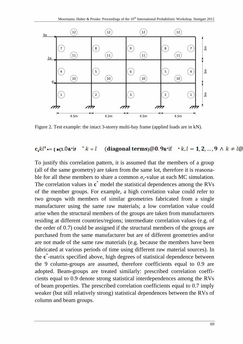
Moormann, Huber & Proske: Proceedings of the 10th International Probabilistic Workshop, Stuttgart 2012
69
3α
4.5m
3m
2α
α
4.5m4.5m
3m
3m
4.5m
12 12 12 12
11 11 11 11
10 10 10 10
1
4
7
2
5
8
3
6
9
1
4
7
2
5
8
Figure 2. Test example: the intact 3-storey multi-bay frame (applied loads are in kN).
To justify this correlation pattern, it is assumed that the members of a group
(all of the same geometry) are taken from the same lot, therefore it is reasona-
ble for all these members to share a common σy-value at each MC simulation.
The correlation values in c* model the statistical dependences among the RVs
of the member groups. For example, a high correlation value could refer to
two groups with members of similar geometries fabricated from a single
manufacturer using the same raw materials; a low correlation value could
arise when the structural members of the groups are taken from manufacturers
residing at different countries/regions; intermediate correlation values (e.g. of
the order of 0.7) could be assigned if the structural members of the groups are
purchased from the same manufacturer but are of different geometries and/or
are not made of the same raw materials (e.g. because the members have been
fabricated at various periods of time using different raw material sources). In
the c*-matrix specified above, high degrees of statistical dependence between
the 9 column-groups are assumed, therefore coefficients equal to 0.9 are
adopted. Beam-groups are treated similarly: prescribed correlation coeffi-
cients equal to 0.9 denote strong statistical interdependences among the RVs
of beam properties. The prescribed correlation coefficients equal to 0.7 imply
weaker (but still relatively strong) statistical dependences between the RVs of
column and beam groups.
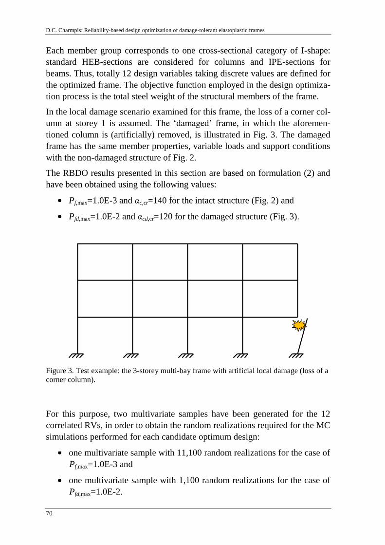
D.C. Charmpis: Reliability-based design optimization of damage-tolerant elastoplastic frames
70
Each member group corresponds to one cross-sectional category of I-shape:
standard HEB-sections are considered for columns and IPE-sections for
beams. Thus, totally 12 design variables taking discrete values are defined for
the optimized frame. The objective function employed in the design optimiza-
tion process is the total steel weight of the structural members of the frame.
In the local damage scenario examined for this frame, the loss of a corner col-
umn at storey 1 is assumed. The ‘damaged’ frame, in which the aforemen-
tioned column is (artificially) removed, is illustrated in Fig. 3. The damaged
frame has the same member properties, variable loads and support conditions
with the non-damaged structure of Fig. 2.
The RBDO results presented in this section are based on formulation (2) and
have been obtained using the following values:
Pf,max=1.0E-3 and αc,cr=140 for the intact structure (Fig. 2) and
Pfd,max=1.0E-2 and αcd,cr=120 for the damaged structure (Fig. 3).
Figure 3. Test example: the 3-storey multi-bay frame with artificial local damage (loss of a
corner column).
For this purpose, two multivariate samples have been generated for the 12
correlated RVs, in order to obtain the random realizations required for the MC
simulations performed for each candidate optimum design:
one multivariate sample with 11,100 random realizations for the case of
Pf,max=1.0E-3 and
one multivariate sample with 1,100 random realizations for the case of
Pfd,max=1.0E-2.
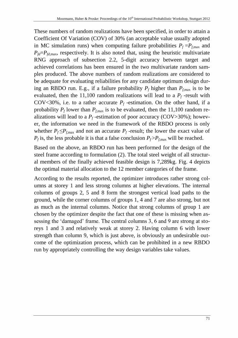
Moormann, Huber & Proske: Proceedings of the 10th International Probabilistic Workshop, Stuttgart 2012
71
These numbers of random realizations have been specified, in order to attain a
Coefficient Of Variation (COV) of 30% (an acceptable value usually adopted
in MC simulation runs) when computing failure probabilities Pf =Pf,max and
Pfd=Pfd,max, respectively. It is also noted that, using the heuristic multivariate
RNG approach of subsection 2.2, 5-digit accuracy between target and
achieved correlations has been ensured in the two multivariate random sam-
ples produced. The above numbers of random realizations are considered to
be adequate for evaluating reliabilities for any candidate optimum design dur-
ing an RBDO run. E.g., if a failure probability Pf higher than Pf,max is to be
evaluated, then the 11,100 random realizations will lead to a Pf -result with
COV<30%, i.e. to a rather accurate Pf -estimation. On the other hand, if a
probability Pf lower than Pf,max is to be evaluated, then the 11,100 random re-
alizations will lead to a Pf -estimation of poor accuracy (COV>30%); howev-
er, the information we need in the framework of the RBDO process is only
whether Pf ≤Pf,max and not an accurate Pf -result; the lower the exact value of
Pf is, the less probable it is that a false conclusion Pf >Pf,max will be reached.
Based on the above, an RBDO run has been performed for the design of the
steel frame according to formulation (2). The total steel weight of all structur-
al members of the finally achieved feasible design is 7,289kg. Fig. 4 depicts
the optimal material allocation to the 12 member categories of the frame.
According to the results reported, the optimizer introduces rather strong col-
umns at storey 1 and less strong columns at higher elevations. The internal
columns of groups 2, 5 and 8 form the strongest vertical load paths to the
ground, while the corner columns of groups 1, 4 and 7 are also strong, but not
as much as the internal columns. Notice that strong columns of group 1 are
chosen by the optimizer despite the fact that one of these is missing when as-
sessing the ‘damaged’ frame. The central columns 3, 6 and 9 are strong at sto-
reys 1 and 3 and relatively weak at storey 2. Having column 6 with lower
strength than column 9, which is just above, is obviously an undesirable out-
come of the optimization process, which can be prohibited in a new RBDO
run by appropriately controlling the way design variables take values.
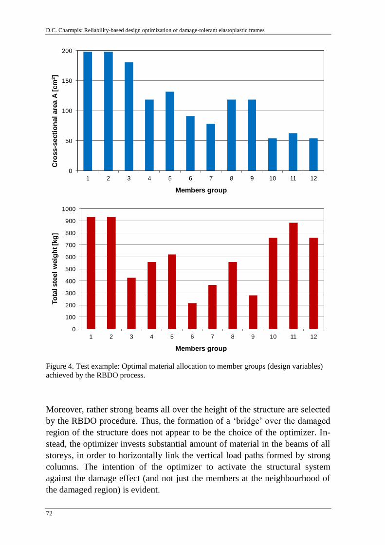
D.C. Charmpis: Reliability-based design optimization of damage-tolerant elastoplastic frames
72
0
50
100
150
200
1 2 3 4 5 6 7 8 9 10 11 12
Cro
ss-s
ecti
on
al
are
a A
[cm
2]
Members group
0
100
200
300
400
500
600
700
800
900
1000
1 2 3 4 5 6 7 8 9 10 11 12
To
tal ste
el
weig
ht [k
g]
Members group
Figure 4. Test example: Optimal material allocation to member groups (design variables)
achieved by the RBDO process.
Moreover, rather strong beams all over the height of the structure are selected
by the RBDO procedure. Thus, the formation of a ‘bridge’ over the damaged
region of the structure does not appear to be the choice of the optimizer. In-
stead, the optimizer invests substantial amount of material in the beams of all
storeys, in order to horizontally link the vertical load paths formed by strong
columns. The intention of the optimizer to activate the structural system
against the damage effect (and not just the members at the neighbourhood of
the damaged region) is evident.

Moormann, Huber & Proske: Proceedings of the 10th International Probabilistic Workshop, Stuttgart 2012
73
6 Concluding remarks
The aim of this work is to study the effect from the incorporation of collapse
resistance requirements into the reliability-based design optimization process
of elastoplastic steel frames. The resulting optimization approach is capable
of producing cost-effective designs with acceptable structural system perfor-
mance under uncertainty.
Inevitably, additional design requirements on system reliability against local
failure will lead to increased structural cost due to the need for extra material
volume/weight. This increase can be quantitatively explored with the present-
ed RBDO approach and the structural elements can be detected, which need
extra material, in order to produce a damage-tolerant structural system.
The results obtained for the test example considered indicate that require-
ments on reliability against local failure are satisfied in the most cost-effective
way by globally activating the structure as a system instead of merely
strengthening members at the neighbourhood of the damaged region. It is
practically impossible to know a-priori the amount and allocation of addition-
al material, in order to optimally satisfy such requirements. Thus, it appears
that an optimization procedure will have to be invoked to cost-effectively
handle any new design problem, as its optimal solution depends on the struc-
tural system considered and its material/geometric properties, the loads acting
on the structure, the demand on collapse resistance and damage tolerance, etc.
References
[1] Agarwal, H.; Renaud, J.E.: Reliability based design optimization using response sur-
faces in application to multidisciplinary systems. Engineering Optimization 36
(2004), pp. 291–311
[2] Allen, M.; Maute, K.: Reliability-based design optimization of aeroelastic structures.
Structural and Multidisciplinary Optimization 27 (2004), pp. 228–242
[3] American Society of Civil Engineers (ASCE): Recommendations for designing col-
lapse-resistant structures. Structural Engineering Institute, Draft Terminology and
Procedures Sub-Committee, 2010
[4] Charmpis, D.C.: Probabilistic structural analysis using random samples with correla-
tions induced by simulated annealing. In: Proceedings of The 2nd International Con-
ference on Soft Computing Technology in Civil, Structural and Environmental
Engineering (CSC 2011), Chania, Crete, Greece, 2011

D.C. Charmpis: Reliability-based design optimization of damage-tolerant elastoplastic frames
74
[5] Charmpis, D.C.; Panteli, P.L.: A heuristic approach for the generation of multivariate
random samples with specified marginal distributions and correlation matrix. Com-
putational Statistics 19 (2004), pp. 283-300
[6] Charmpis, D.C.; Schuëller, G.I.: Coping with physical uncertainties in structural me-
chanics: uncertainties modeling, methods of analysis and applications. In: Marti, K.;
Ermoliev, Y.; Makowski, M.; Pflug, G. (editors): Coping with Uncertainty – Model-
ing and Policy Issues. Vol. 581 of Lecture Notes in Economics and Mathematical
Systems, Springer, 2006, pp. 67-83
[7] Department of Defence (DoD): Unified facilities criteria (UFC), design of buildings
to resist progressive collapse. UFC 4-023-03, Washington D.C., 2005
[8] General Services Administration (GSA): Progressive collapse analysis and design
guidelines for new federal office buildings and major modernization projects. Wash-
ington D.C., 2003
[9] Kontogiannis, A.; Charmpis, D.C.: Sizing optimization of collapse-resistant frames.
In: Proceedings of 7th GRACM International Congress on Computational Mechanics
(GRACM 2011), Athens, Greece, 2011
[10] Papadrakakis, M.; Lagaros, N.D.: Reliability-based structural optimization using
neural networks and Monte Carlo simulation. Computer Methods in Applied Me-
chanics and Engineering 191 (2002), pp. 3491-3507
[11] Royset, J.O.; Der Kiureghian, A.; Polak, E.: Reliability-based optimal design of se-
ries structural systems. ASCE Journal of Engineering Mechanics 127 (2001), pp.
607-614
[12] Sørensen, J.D.; Christensen, H.H.: Danish requirements for robustness of structures:
background and implementation. Structural Engineering International 16 (2006), pp.
172-177
[13] Starossek, U.; Wolf, M.: Design of collapse-resistant structures. In: Proceedings of
JCSS and IABSE Workshop on Robustness of Structures, Building Research Estab-
lishment, Garston, Watford, UK, 2005
[14] Tsompanakis, Y.; Papadrakakis, M.: Large-scale reliability-based structural optimi-
zation. Structural and Multidisciplinary Optimization 26 (2004), pp. 429–440
[15] Wong, M.B.: Plastic analysis and design of steel structures. Butterworth-
Heinemann, Elsevier, 2009
[16] Yi, P.; Cheng, G.; Jiang, L.: A sequential approximate programming strategy for
performance-measure-based probabilistic structural design optimization. Structural
Safety 30 (2008), pp. 91-109

Moormann, Huber & Proske: Proceedings of the 10th International Probabilistic Workshop, Stuttgart 2012
75
Seemingly contradictory: influence of stress-
reduction-methods on the strength of bonded
joints composed of brittle adherends
Till Vallée1, Thomas Tannert
2 & Cordula Grunwald
1
1Fraunhofer-Institut für Fertigungstechnik und Angewandte Material-
forschung, IFAM, Wiener Straße 12, 28359 Bremen/Germany 2 The University of British Columbia, 2424 Main Mall,
Vancouver, BC, V6T1Z4, Canada
Abstract: Adhesively bonded joints are increasingly considered for structural
applications in engineering. Because of the associated mechanical singularity,
their dimensioning remains a challenge, especially if considering brittle ad-
herends. The influence of stress-reduction-methods on their strength was inves-
tigated herein: experimental and numerical investigations were carried out on
two types of brittle adherends considering three different stress-reduction
methods. Although numerical analyses showed that the stress peaks are re-
duced, the experimental evidence lacked the corresponding strength increase,
despite intuition and common sense. A probabilistic strength prediction method
subsequently applied explains most of the seemingly contradictory findings.
The presented work allows for a better insight into the relation between stress-
reduction and strength increase of adhesively bonded joints, which is greatly
affected by the brittleness of the adherends.
1 Introduction
Adhesively bonding represents a joining technique that is increasingly com-
peting with mechanical fasteners (bolts, rivets) and welding. Initially pushed
by the aeronautical and automotive industries, adhesively bonding is gradual-
ly considered in civil engineering applications, especially in combination with
fibrous and anisotropic materials as composites and timber. Since load trans-
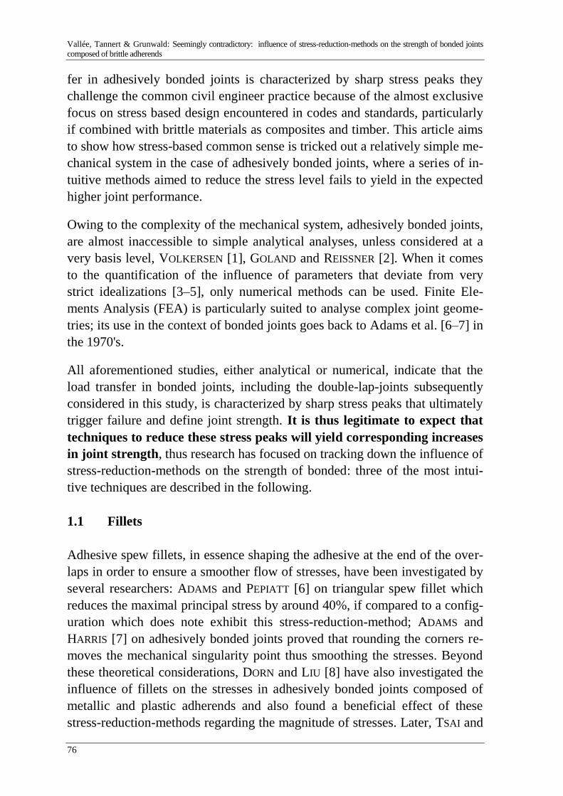
Vallée, Tannert & Grunwald: Seemingly contradictory: influence of stress-reduction-methods on the strength of bonded joints
composed of brittle adherends
76
fer in adhesively bonded joints is characterized by sharp stress peaks they
challenge the common civil engineer practice because of the almost exclusive
focus on stress based design encountered in codes and standards, particularly
if combined with brittle materials as composites and timber. This article aims
to show how stress-based common sense is tricked out a relatively simple me-
chanical system in the case of adhesively bonded joints, where a series of in-
tuitive methods aimed to reduce the stress level fails to yield in the expected
higher joint performance.
Owing to the complexity of the mechanical system, adhesively bonded joints,
are almost inaccessible to simple analytical analyses, unless considered at a
very basis level, VOLKERSEN [1], GOLAND and REISSNER [2]. When it comes
to the quantification of the influence of parameters that deviate from very
strict idealizations [3–5], only numerical methods can be used. Finite Ele-
ments Analysis (FEA) is particularly suited to analyse complex joint geome-
tries; its use in the context of bonded joints goes back to Adams et al. [6–7] in
the 1970's.
All aforementioned studies, either analytical or numerical, indicate that the
load transfer in bonded joints, including the double-lap-joints subsequently
considered in this study, is characterized by sharp stress peaks that ultimately
trigger failure and define joint strength. It is thus legitimate to expect that
techniques to reduce these stress peaks will yield corresponding increases
in joint strength, thus research has focused on tracking down the influence of
stress-reduction-methods on the strength of bonded: three of the most intui-
tive techniques are described in the following.
1.1 Fillets
Adhesive spew fillets, in essence shaping the adhesive at the end of the over-
laps in order to ensure a smoother flow of stresses, have been investigated by
several researchers: ADAMS and PEPIATT [6] on triangular spew fillet which
reduces the maximal principal stress by around 40%, if compared to a config-
uration which does note exhibit this stress-reduction-method; ADAMS and
HARRIS [7] on adhesively bonded joints proved that rounding the corners re-
moves the mechanical singularity point thus smoothing the stresses. Beyond
these theoretical considerations, DORN and LIU [8] have also investigated the
influence of fillets on the stresses in adhesively bonded joints composed of
metallic and plastic adherends and also found a beneficial effect of these
stress-reduction-methods regarding the magnitude of stresses. Later, TSAI and
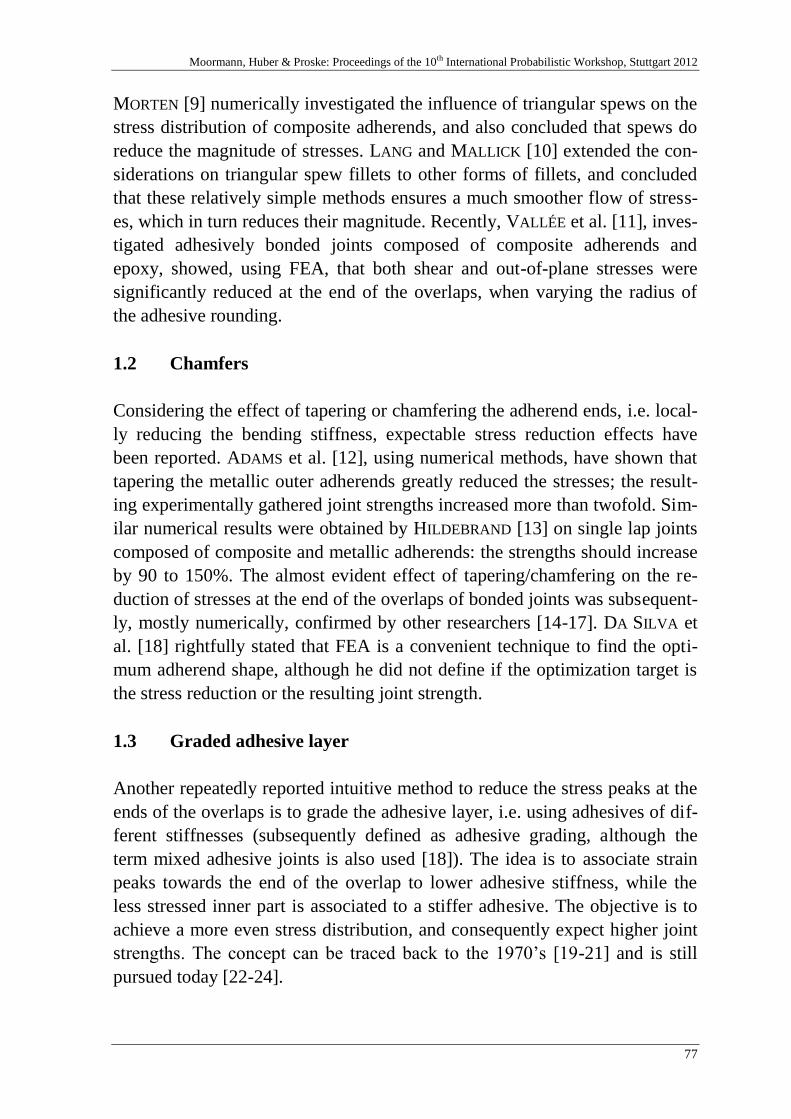
Moormann, Huber & Proske: Proceedings of the 10th International Probabilistic Workshop, Stuttgart 2012
77
MORTEN [9] numerically investigated the influence of triangular spews on the
stress distribution of composite adherends, and also concluded that spews do
reduce the magnitude of stresses. LANG and MALLICK [10] extended the con-
siderations on triangular spew fillets to other forms of fillets, and concluded
that these relatively simple methods ensures a much smoother flow of stress-
es, which in turn reduces their magnitude. Recently, VALLÉE et al. [11], inves-
tigated adhesively bonded joints composed of composite adherends and
epoxy, showed, using FEA, that both shear and out-of-plane stresses were
significantly reduced at the end of the overlaps, when varying the radius of
the adhesive rounding.
1.2 Chamfers
Considering the effect of tapering or chamfering the adherend ends, i.e. local-
ly reducing the bending stiffness, expectable stress reduction effects have
been reported. ADAMS et al. [12], using numerical methods, have shown that
tapering the metallic outer adherends greatly reduced the stresses; the result-
ing experimentally gathered joint strengths increased more than twofold. Sim-
ilar numerical results were obtained by HILDEBRAND [13] on single lap joints
composed of composite and metallic adherends: the strengths should increase
by 90 to 150%. The almost evident effect of tapering/chamfering on the re-
duction of stresses at the end of the overlaps of bonded joints was subsequent-
ly, mostly numerically, confirmed by other researchers [14-17]. DA SILVA et
al. [18] rightfully stated that FEA is a convenient technique to find the opti-
mum adherend shape, although he did not define if the optimization target is
the stress reduction or the resulting joint strength.
1.3 Graded adhesive layer
Another repeatedly reported intuitive method to reduce the stress peaks at the
ends of the overlaps is to grade the adhesive layer, i.e. using adhesives of dif-
ferent stiffnesses (subsequently defined as adhesive grading, although the
term mixed adhesive joints is also used [18]). The idea is to associate strain
peaks towards the end of the overlap to lower adhesive stiffness, while the
less stressed inner part is associated to a stiffer adhesive. The objective is to
achieve a more even stress distribution, and consequently expect higher joint
strengths. The concept can be traced back to the 1970’s [19-21] and is still
pursued today [22-24].
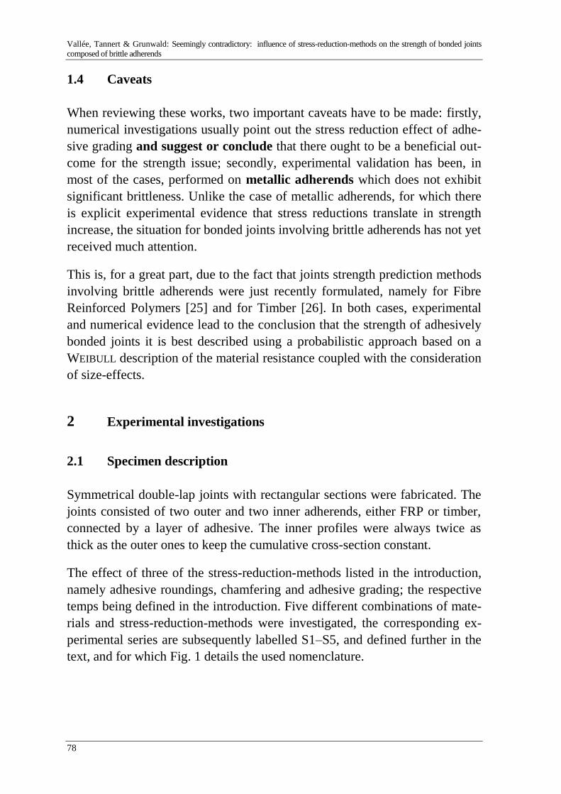
Vallée, Tannert & Grunwald: Seemingly contradictory: influence of stress-reduction-methods on the strength of bonded joints
composed of brittle adherends
78
1.4 Caveats
When reviewing these works, two important caveats have to be made: firstly,
numerical investigations usually point out the stress reduction effect of adhe-
sive grading and suggest or conclude that there ought to be a beneficial out-
come for the strength issue; secondly, experimental validation has been, in
most of the cases, performed on metallic adherends which does not exhibit
significant brittleness. Unlike the case of metallic adherends, for which there
is explicit experimental evidence that stress reductions translate in strength
increase, the situation for bonded joints involving brittle adherends has not yet
received much attention.
This is, for a great part, due to the fact that joints strength prediction methods
involving brittle adherends were just recently formulated, namely for Fibre
Reinforced Polymers [25] and for Timber [26]. In both cases, experimental
and numerical evidence lead to the conclusion that the strength of adhesively
bonded joints it is best described using a probabilistic approach based on a
WEIBULL description of the material resistance coupled with the consideration
of size-effects.
2 Experimental investigations
2.1 Specimen description
Symmetrical double-lap joints with rectangular sections were fabricated. The
joints consisted of two outer and two inner adherends, either FRP or timber,
connected by a layer of adhesive. The inner profiles were always twice as
thick as the outer ones to keep the cumulative cross-section constant.
The effect of three of the stress-reduction-methods listed in the introduction,
namely adhesive roundings, chamfering and adhesive grading; the respective
temps being defined in the introduction. Five different combinations of mate-
rials and stress-reduction-methods were investigated, the corresponding ex-
perimental series are subsequently labelled S1–S5, and defined further in the
text, and for which Fig. 1 details the used nomenclature.
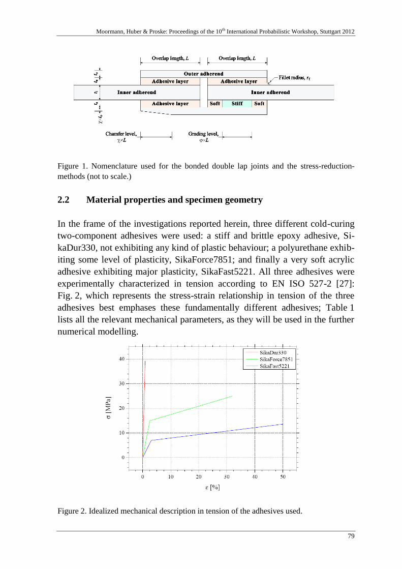
Moormann, Huber & Proske: Proceedings of the 10th International Probabilistic Workshop, Stuttgart 2012
79
Figure 1. Nomenclature used for the bonded double lap joints and the stress-reduction-
methods (not to scale.)
2.2 Material properties and specimen geometry
In the frame of the investigations reported herein, three different cold-curing
two-component adhesives were used: a stiff and brittle epoxy adhesive, Si-
kaDur330, not exhibiting any kind of plastic behaviour; a polyurethane exhib-
iting some level of plasticity, SikaForce7851; and finally a very soft acrylic
adhesive exhibiting major plasticity, SikaFast5221. All three adhesives were
experimentally characterized in tension according to EN ISO 527-2 [27]:
Fig. 2, which represents the stress-strain relationship in tension of the three
adhesives best emphases these fundamentally different adhesives; Table 1
lists all the relevant mechanical parameters, as they will be used in the further
numerical modelling.
Figure 2. Idealized mechanical description in tension of the adhesives used.
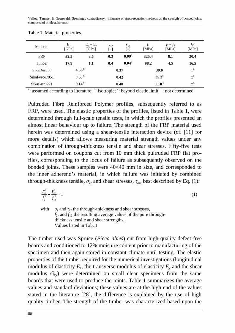
Vallée, Tannert & Grunwald: Seemingly contradictory: influence of stress-reduction-methods on the strength of bonded joints
composed of brittle adherends
80
Table 1. Material properties.
Material Ex
[GPa]
Ey = Ez
[GPa] xz
[–] yz
[–]
f1
[MPa]
f2 = f3
[MPa]
f12
[MPa]
FRP 32.5 3.5 0.3 0.09a 325.4 8.1 20.4
Timber 17.9 1.1 0.4 0.04a 98.2 4.5 16.5
SikaDur330 4.56 b 0.37 39.0 □
d
SikaForce7851 0.58 b
0.42 25.3c □
d
SikaFast5221 0.14 b 0.40 11.8
c □
d
a: assumed according to literature;
b: isotropic;
c: beyond elastic limit;
d: not determined
Pultruded Fibre Reinforced Polymer profiles, subsequently referred to as
FRP, were used. The elastic properties of the profiles, listed in Table 1, were
determined through full-scale tensile tests, in which the profiles presented an
almost linear behaviour up to failure. The strength of the FRP material used
herein was determined using a shear-tensile interaction device (cf. [11] for
more details) which allows measuring material strength values under any
combination of through-thickness tensile and shear stresses. Fifty-five tests
were performed on coupons cut from 10 mm thick pultruded FRP flat pro-
files, corresponding to the locus of failure as subsequently observed on the
bonded joints. These samples were 40×40 mm in size, and corresponded to
the inner adherend’s material, in which failure was initiated by combined
through-thickness tensile, σz, and shear stresses, τxz, best described by Eq. (1):
22
2 2
2 12
1xzz
f f (1)
with σz and τxz the through-thickness and shear stresses,
f2, and f12 the resulting average values of the pure through-
thickness tensile and shear strengths,
Values listed in Tab. 1
The timber used was Spruce (Picea abies) cut from high quality defect-free
boards and conditioned to 12% moisture content prior to manufacturing of the
specimen and then again stored in constant climate until testing. The elastic
properties of the timber required for the numerical investigations (longitudinal
modulus of elasticity Ex, the transverse modulus of elasticity Ey and the shear
modulus Gxy) were determined on small clear specimens from the same
boards that were used to produce the joints. Table 1 summarizes the average
values and standard deviations; these values are at the high end of the values
stated in the literature [28], the difference is explained by the use of high
quality timber. The strength of the timber was characterized based upon the
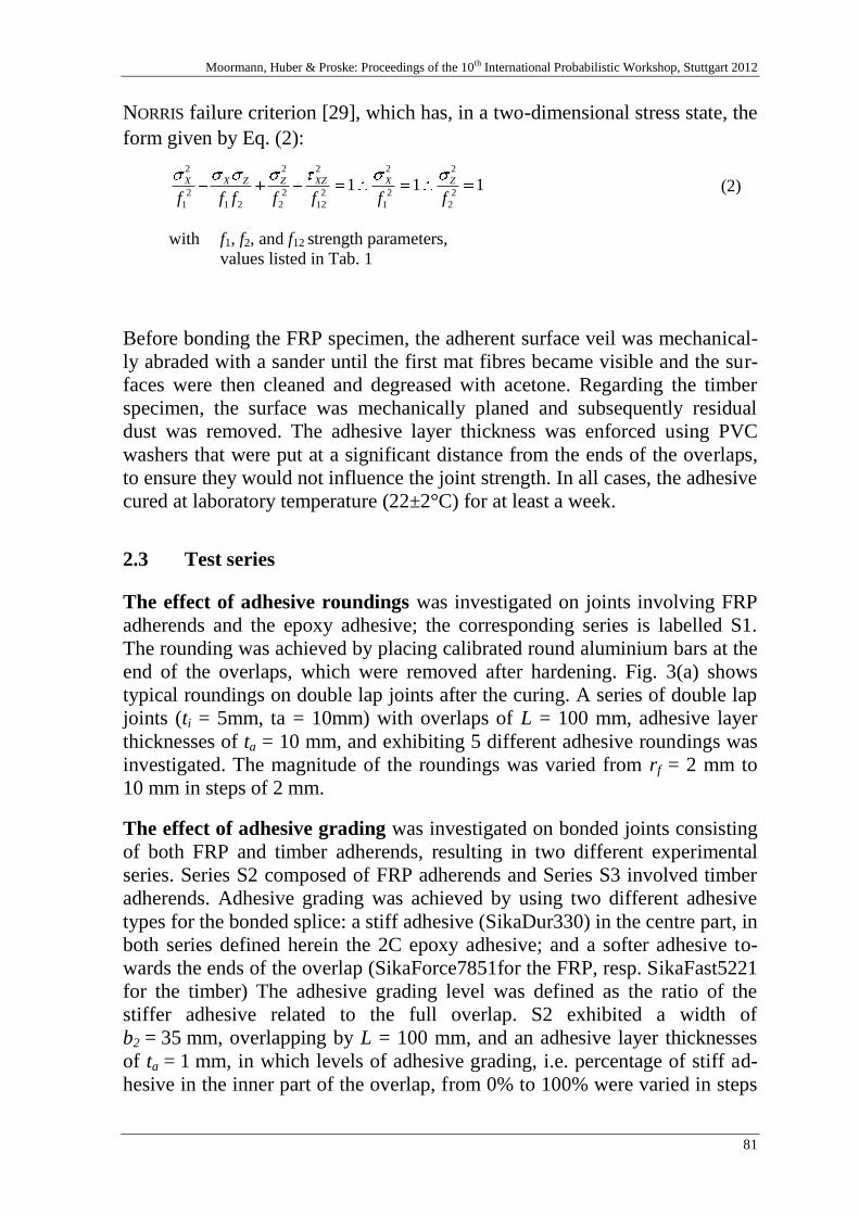
Moormann, Huber & Proske: Proceedings of the 10th International Probabilistic Workshop, Stuttgart 2012
81
NORRIS failure criterion [29], which has, in a two-dimensional stress state, the
form given by Eq. (2):
1112
2
2
2
1
2
2
12
2
2
2
2
21
2
1
2
fffffff
ZXXZZZXX (2)
with f1, f2, and f12 strength parameters,
values listed in Tab. 1
Before bonding the FRP specimen, the adherent surface veil was mechanical-
ly abraded with a sander until the first mat fibres became visible and the sur-
faces were then cleaned and degreased with acetone. Regarding the timber
specimen, the surface was mechanically planed and subsequently residual
dust was removed. The adhesive layer thickness was enforced using PVC
washers that were put at a significant distance from the ends of the overlaps,
to ensure they would not influence the joint strength. In all cases, the adhesive
cured at laboratory temperature (22±2°C) for at least a week.
2.3 Test series
The effect of adhesive roundings was investigated on joints involving FRP
adherends and the epoxy adhesive; the corresponding series is labelled S1.
The rounding was achieved by placing calibrated round aluminium bars at the
end of the overlaps, which were removed after hardening. Fig. 3(a) shows
typical roundings on double lap joints after the curing. A series of double lap
joints (ti = 5mm, ta = 10mm) with overlaps of L = 100 mm, adhesive layer
thicknesses of ta = 10 mm, and exhibiting 5 different adhesive roundings was
investigated. The magnitude of the roundings was varied from rf = 2 mm to
10 mm in steps of 2 mm.
The effect of adhesive grading was investigated on bonded joints consisting
of both FRP and timber adherends, resulting in two different experimental
series. Series S2 composed of FRP adherends and Series S3 involved timber
adherends. Adhesive grading was achieved by using two different adhesive
types for the bonded splice: a stiff adhesive (SikaDur330) in the centre part, in
both series defined herein the 2C epoxy adhesive; and a softer adhesive to-
wards the ends of the overlap (SikaForce7851for the FRP, resp. SikaFast5221
for the timber) The adhesive grading level was defined as the ratio of the
stiffer adhesive related to the full overlap. S2 exhibited a width of
b2 = 35 mm, overlapping by L = 100 mm, and an adhesive layer thicknesses
of ta = 1 mm, in which levels of adhesive grading, i.e. percentage of stiff ad-
hesive in the inner part of the overlap, from 0% to 100% were varied in steps
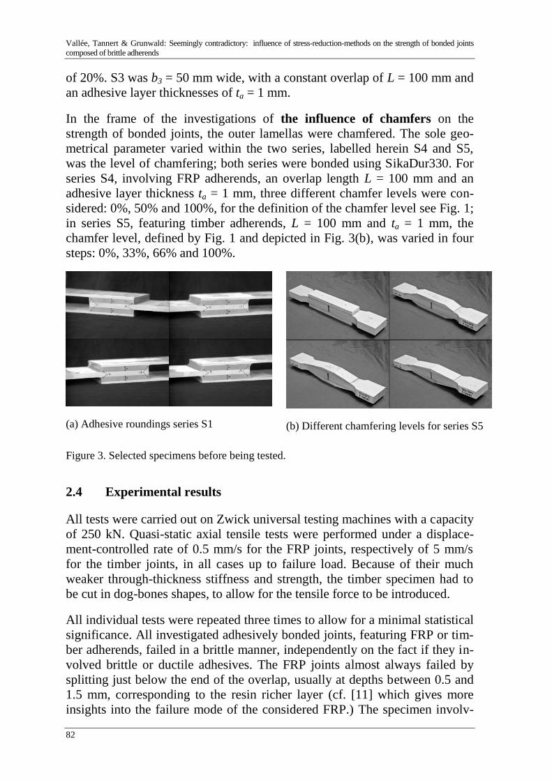
Vallée, Tannert & Grunwald: Seemingly contradictory: influence of stress-reduction-methods on the strength of bonded joints
composed of brittle adherends
82
of 20%. S3 was b3 = 50 mm wide, with a constant overlap of L = 100 mm and
an adhesive layer thicknesses of ta = 1 mm.
In the frame of the investigations of the influence of chamfers on the
strength of bonded joints, the outer lamellas were chamfered. The sole geo-
metrical parameter varied within the two series, labelled herein S4 and S5,
was the level of chamfering; both series were bonded using SikaDur330. For
series S4, involving FRP adherends, an overlap length L = 100 mm and an
adhesive layer thickness ta = 1 mm, three different chamfer levels were con-
sidered: 0%, 50% and 100%, for the definition of the chamfer level see Fig. 1;
in series S5, featuring timber adherends, L = 100 mm and ta = 1 mm, the
chamfer level, defined by Fig. 1 and depicted in Fig. 3(b), was varied in four
steps: 0%, 33%, 66% and 100%.
(a) Adhesive roundings series S1
(b) Different chamfering levels for series S5
Figure 3. Selected specimens before being tested.
2.4 Experimental results
All tests were carried out on Zwick universal testing machines with a capacity
of 250 kN. Quasi-static axial tensile tests were performed under a displace-
ment-controlled rate of 0.5 mm/s for the FRP joints, respectively of 5 mm/s
for the timber joints, in all cases up to failure load. Because of their much
weaker through-thickness stiffness and strength, the timber specimen had to
be cut in dog-bones shapes, to allow for the tensile force to be introduced.
All individual tests were repeated three times to allow for a minimal statistical
significance. All investigated adhesively bonded joints, featuring FRP or tim-
ber adherends, failed in a brittle manner, independently on the fact if they in-
volved brittle or ductile adhesives. The FRP joints almost always failed by
splitting just below the end of the overlap, usually at depths between 0.5 and
1.5 mm, corresponding to the resin richer layer (cf. [11] which gives more
insights into the failure mode of the considered FRP.) The specimen involv-
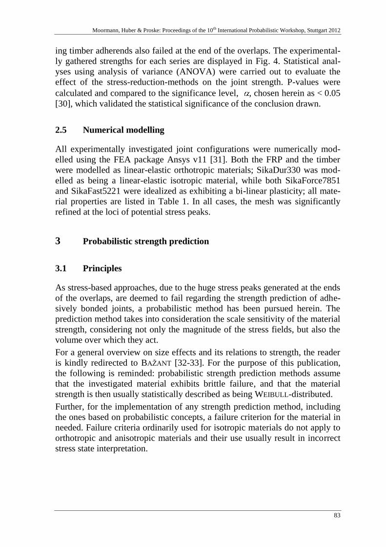
Moormann, Huber & Proske: Proceedings of the 10th International Probabilistic Workshop, Stuttgart 2012
83
ing timber adherends also failed at the end of the overlaps. The experimental-
ly gathered strengths for each series are displayed in Fig. 4. Statistical anal-
yses using analysis of variance (ANOVA) were carried out to evaluate the
effect of the stress-reduction-methods on the joint strength. P-values were
calculated and compared to the significance level, , chosen herein as < 0.05
[30], which validated the statistical significance of the conclusion drawn.
2.5 Numerical modelling
All experimentally investigated joint configurations were numerically mod-
elled using the FEA package Ansys v11 [31]. Both the FRP and the timber
were modelled as linear-elastic orthotropic materials; SikaDur330 was mod-
elled as being a linear-elastic isotropic material, while both SikaForce7851
and SikaFast5221 were idealized as exhibiting a bi-linear plasticity; all mate-
rial properties are listed in Table 1. In all cases, the mesh was significantly
refined at the loci of potential stress peaks.
3 Probabilistic strength prediction
3.1 Principles
As stress-based approaches, due to the huge stress peaks generated at the ends
of the overlaps, are deemed to fail regarding the strength prediction of adhe-
sively bonded joints, a probabilistic method has been pursued herein. The
prediction method takes into consideration the scale sensitivity of the material
strength, considering not only the magnitude of the stress fields, but also the
volume over which they act.
For a general overview on size effects and its relations to strength, the reader
is kindly redirected to BAŽANT [32-33]. For the purpose of this publication,
the following is reminded: probabilistic strength prediction methods assume
that the investigated material exhibits brittle failure, and that the material
strength is then usually statistically described as being WEIBULL-distributed.
Further, for the implementation of any strength prediction method, including
the ones based on probabilistic concepts, a failure criterion for the material in
needed. Failure criteria ordinarily used for isotropic materials do not apply to
orthotropic and anisotropic materials and their use usually result in incorrect
stress state interpretation.
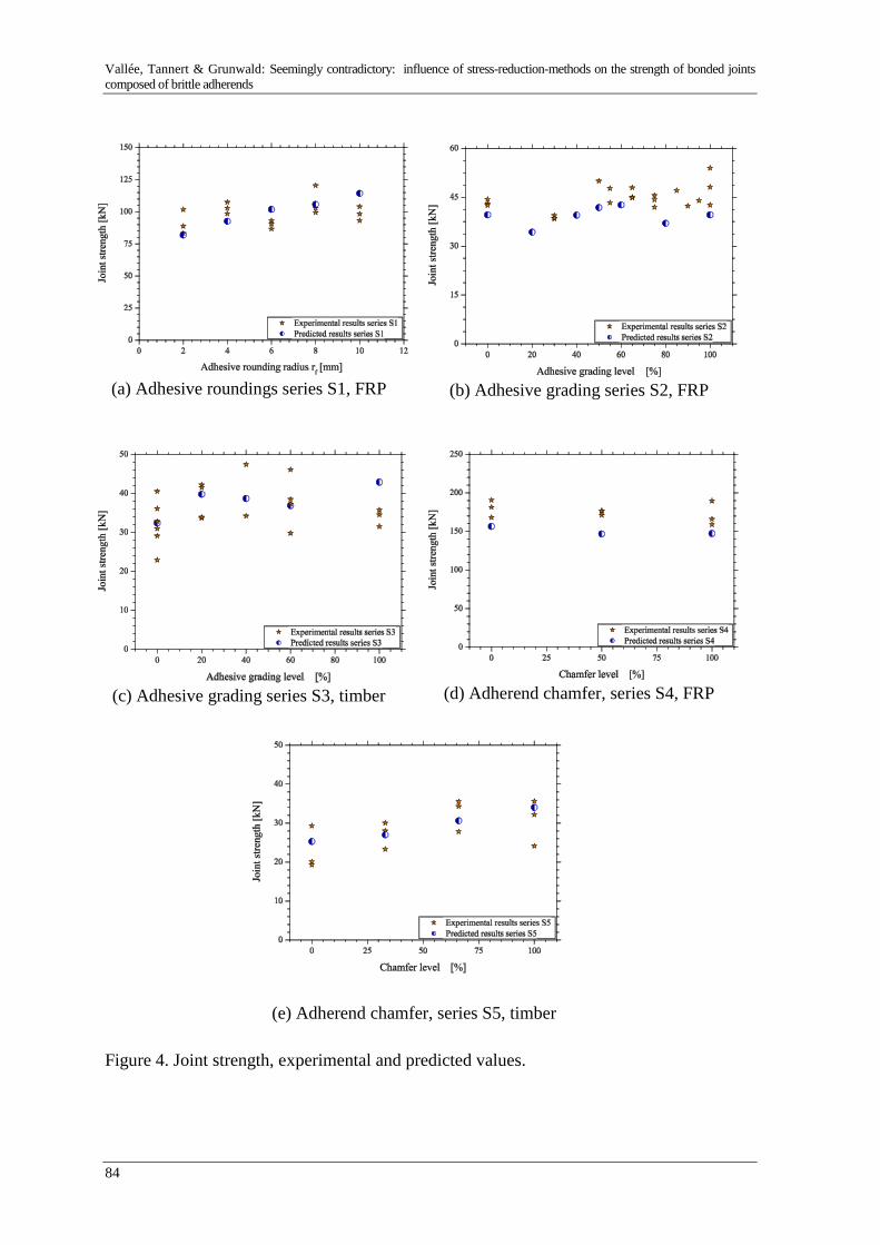
Vallée, Tannert & Grunwald: Seemingly contradictory: influence of stress-reduction-methods on the strength of bonded joints
composed of brittle adherends
84
(a) Adhesive roundings series S1, FRP (b) Adhesive grading series S2, FRP
(c) Adhesive grading series S3, timber (d) Adherend chamfer, series S4, FRP
(e) Adherend chamfer, series S5, timber
Figure 4. Joint strength, experimental and predicted values.
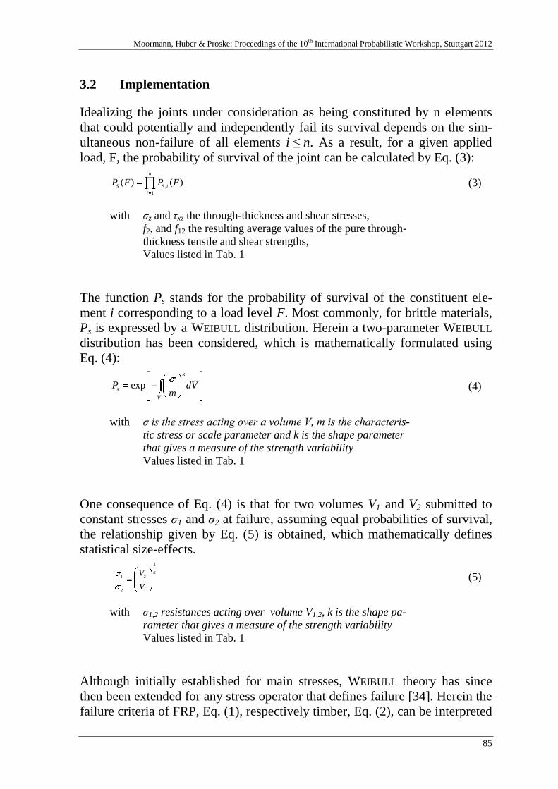
Moormann, Huber & Proske: Proceedings of the 10th International Probabilistic Workshop, Stuttgart 2012
85
3.2 Implementation
Idealizing the joints under consideration as being constituted by n elements
that could potentially and independently fail its survival depends on the sim-
ultaneous non-failure of all elements i ≤ n. As a result, for a given applied
load, F, the probability of survival of the joint can be calculated by Eq. (3):
,
1
( ) ( )n
S S i
i
P F P F
(3)
with σz and τxz the through-thickness and shear stresses,
f2, and f12 the resulting average values of the pure through-
thickness tensile and shear strengths,
Values listed in Tab. 1
The function Ps stands for the probability of survival of the constituent ele-
ment i corresponding to a load level F. Most commonly, for brittle materials,
Ps is expressed by a WEIBULL distribution. Herein a two-parameter WEIBULL
distribution has been considered, which is mathematically formulated using
Eq. (4):
exp
k
s
V
P dVm
(4)
with σ is the stress acting over a volume V, m is the characteris-
tic stress or scale parameter and k is the shape parameter
that gives a measure of the strength variability
Values listed in Tab. 1
One consequence of Eq. (4) is that for two volumes V1 and V2 submitted to
constant stresses σ1 and σ2 at failure, assuming equal probabilities of survival,
the relationship given by Eq. (5) is obtained, which mathematically defines
statistical size-effects.
1 2
2 1
1
kV
V
(5)
with σ1,2 resistances acting over volume V1,2, k is the shape pa-
rameter that gives a measure of the strength variability
Values listed in Tab. 1
Although initially established for main stresses, WEIBULL theory has since
then been extended for any stress operator that defines failure [34]. Herein the
failure criteria of FRP, Eq. (1), respectively timber, Eq. (2), can be interpreted
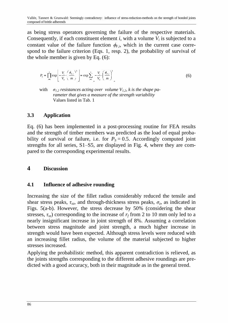
Vallée, Tannert & Grunwald: Seemingly contradictory: influence of stress-reduction-methods on the strength of bonded joints
composed of brittle adherends
86
as being stress operators governing the failure of the respective materials.
Consequently, if each constituent element i, with a volume Vi is subjected to a
constant value of the failure function F,i, which in the current case corre-
spond to the failure criterion (Eqs. 1, resp. 2), the probability of survival of
the whole member is given by Eq. (6):
, ,
11 0 0
exp exp
k kn n
F i F ii i
S
ii
V VP
V m V m
(6)
with σ1,2 resistances acting over volume V1,2, k is the shape pa-
rameter that gives a measure of the strength variability
Values listed in Tab. 1
3.3 Application
Eq. (6) has been implemented in a post-processing routine for FEA results
and the strength of timber members was predicted as the load of equal proba-
bility of survival or failure, i.e. for PS = 0.5. Accordingly computed joint
strengths for all series, S1–S5, are displayed in Fig. 4, where they are com-
pared to the corresponding experimental results.
4 Discussion
4.1 Influence of adhesive rounding
Increasing the size of the fillet radius considerably reduced the tensile and
shear stress peaks, τxz, and through-thickness stress peaks, σz, as indicated in
Figs. 5(a-b). However, the stress decrease by 50% (considering the shear
stresses, τxz) corresponding to the increase of rf from 2 to 10 mm only led to a
nearly insignificant increase in joint strength of 8%. Assuming a correlation
between stress magnitude and joint strength, a much higher increase in
strength would have been expected. Although stress levels were reduced with
an increasing fillet radius, the volume of the material subjected to higher
stresses increased.
Applying the probabilistic method, this apparent contradiction is relieved, as
the joints strengths corresponding to the different adhesive roundings are pre-
dicted with a good accuracy, both in their magnitude as in the general trend.
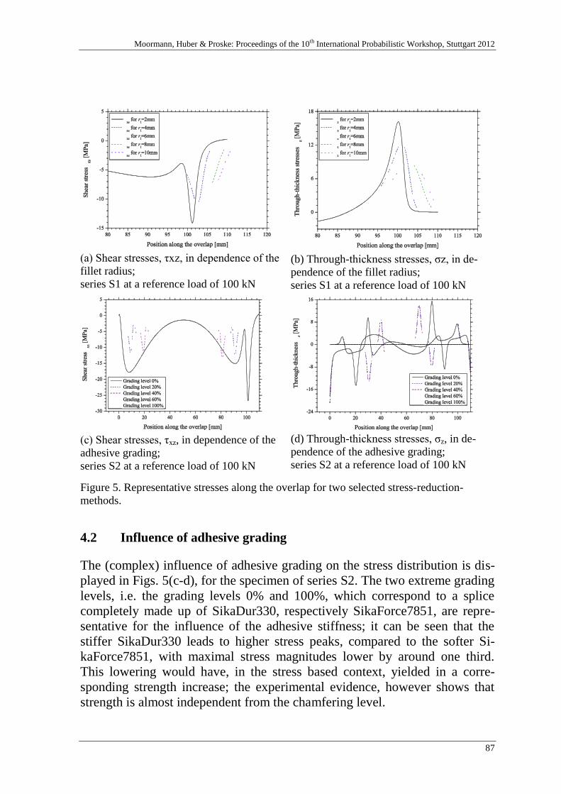
Moormann, Huber & Proske: Proceedings of the 10th International Probabilistic Workshop, Stuttgart 2012
87
(a) Shear stresses, τxz, in dependence of the
fillet radius;
series S1 at a reference load of 100 kN
(b) Through-thickness stresses, σz, in de-
pendence of the fillet radius;
series S1 at a reference load of 100 kN
(c) Shear stresses, τxz, in dependence of the
adhesive grading;
series S2 at a reference load of 100 kN
(d) Through-thickness stresses, σz, in de-
pendence of the adhesive grading;
series S2 at a reference load of 100 kN
Figure 5. Representative stresses along the overlap for two selected stress-reduction-
methods.
4.2 Influence of adhesive grading
The (complex) influence of adhesive grading on the stress distribution is dis-
played in Figs. 5(c-d), for the specimen of series S2. The two extreme grading
levels, i.e. the grading levels 0% and 100%, which correspond to a splice
completely made up of SikaDur330, respectively SikaForce7851, are repre-
sentative for the influence of the adhesive stiffness; it can be seen that the
stiffer SikaDur330 leads to higher stress peaks, compared to the softer Si-
kaForce7851, with maximal stress magnitudes lower by around one third.
This lowering would have, in the stress based context, yielded in a corre-
sponding strength increase; the experimental evidence, however shows that
strength is almost independent from the chamfering level.
Vallée, Tannert & Grunwald: Seemingly contradictory: influence of stress-reduction-methods on the strength of bonded joints
composed of brittle adherends
88
The probabilistic method on the other hand delivers predictions that are rea-
sonably consistent with the experimental data.
4.3 Influence of chamfering
Similarly to the adhesive rounding, chamfering does significantly reduce the
magnitude of the shear stress peaks, τxz, and through-thickness stress peaks, σz,
(not shown for constraints of space in this paper.) For the case of FRP: by ap-
prox. 40% if comparing the shear stresses, τxz, of the joints exhibiting no
chamfering relatively to a chamfering level of 100%. However, the corre-
sponding experimentally determined joint strengths were not affected by this
particular stress reduction, as clearly indicated by Figs. 4(d-e).
Here again, taking into account the fact that the joint strength is not only driv-
en by the magnitude of stresses, but also by their distribution, i.e. applying a
probabilistic approach, sheds light onto this apparent inconsistency by pre-
dicting joint strengths that are in good agreement with the experimental val-
ues.
5 Conclusion
Adhesively bonded joints are characterized by sharp stress peaks towards the
ends of the overlaps, which trigger failure, thus defining strength. A repeated-
ly reported and at first sight intuitive method to increase the strength of these
elements is to reduce the stress peaks by either acting on the geometry, e.g.
chamfering the adherends or implementing fillets in the adhesive layer, or on
the adhesive, e.g. using ductile adhesives or grading them.
Regarding brittle adherends, i.e. FRP and timber, three commonly reported
methods to reduce stress magnitudes, i.e. chamfering, ductile adhesives, and
adhesive grading, were experimentally and numerically investigated. These
investigations, pursued on a wide range of parameters resulting in five differ-
ent experimental series, allowed for the following observations:
1. All of the investigated stress-reduction-methods do, according to FEA,
lead to significant stress reductions, yet the so reduced stresses act on
larger volumes of the adherends;
2. All experimentally investigated adhesively bonded joints failed in a
brittle manner, so the materials they were constituted of;
3. None of the investigated stress-reduction-method, neither for FRP nor
for timber, did significantly increase the experimentally determined
joint strength.

Moormann, Huber & Proske: Proceedings of the 10th International Probabilistic Workshop, Stuttgart 2012
89
The latter listed observations did allow drawing the following conclusions:
4. There is no direct correlation between stress magnitude and failure,
even considering a verified failure criterion, when dealing with brittle
materials;
5. Thus, direct stress based approaches to predict the strength of adhesive-
ly bonded joints composed of brittle adherends are not suited for di-
mensioning purposes.
Considering the aforementioned, the authors computationally developed a
probabilistic strength prediction method, which implemented a statistical
based formulation of size-effects. The probabilistic method not only offers a
comprehensive a mechanically coherent for the seemingly contradictory rela-
tion between stress reduction and lack of corresponding joint strength in-
crease, it also delivers consistently accurate joint strength estimates for all
considered experimental series which makes it useful for their dimensioning.
6 Literature
[1] O. VOLKERSEN, Recherches sur la théorie des assemblages collés, Constr. Metall.
(1965) 4:3-13.
[2] M. GOLAND, E. REISSNER, The stresses in cemented joints, J. Appl. Mech. (1944)
A17-27.
[3] C. RAPHAEL, Variable-adhesive bonded joints, Appl. Polym. Symp. 3 (1966) 99-108.
[4] L.J. HART-SMITH, Analysis and design of advanced composite bonded joints. NASA
CR-2218, 1974.
[5] W.J. RENTON, J.R. VINSON, The efficient design of adhesive bonded joints, J. Adhes.
7 (1975) 175-193.
[6] R.D. ADAMS, N.A. PEPIATT, Stress analysis of adhesive bonded lab joints, J. Strain
Anal. 9 (1974) 185-196.
[7] R.D. ADAMS, J.A. HARRIS, The influence of local geometry on the strength of adhe-
sive joints. Int. J. Adhes. Adhes. 7 (1987) 69-80.
[8] L. DORN, W. LIU, The stress state and failure properties of adhesive bonded plas-
tic/metal joints, Int. J. Adhes. Adhes. 13 (1993) 21-31.
[9] M.Y. TSAI, J. MORTON, The effect of a spew fillet on adhesive stress distributions in
laminated composite single-lap joints, Compos. Struct. 32 (1995) 123-31.
[10] T.P. LANG, P.K. MALLICK, Effect of spew geometry on stresses in single lap adhesive
joints. Int. J. Adhes. Adhes. 18 (1998) 167-77.
[11] T. VALLÉE, J.R. CORREIA, T. KELLER, Probabilistic strength prediction for double lap
joints composed of GFRP profiles, Part I: experimental and numerical Investigations.
Compos. Sc. Tech. 66 (2006) 1903-1914.
[12] R.D. ADAMS, R.W. ATKINS, J.A. HARRIS, A.J. KINLOCH, Stress-analysis and failure
properties of carbon-fiber-reinforced-plastic steel double-lap joints, J. Adhes. 20
(1986) 29-53.
Vallée, Tannert & Grunwald: Seemingly contradictory: influence of stress-reduction-methods on the strength of bonded joints
composed of brittle adherends
90
[13] M. HILDEBRAND, Non-linear analysis and optimization of adhesively bonded single
lap joints between fibre-reinforced plastics and metals, Int. J. Adhes. Adhes. 14
(1994) 261-267.
[14] S. AMIJIMA, T. FUJII, A simple stress analysis method for adhesive bonded tapered
joints, Int. J. Adhes. Adhes. 9 (1989) 155-160.
[15] E. SANCAKTAR, P. NIRANTAR, Increasing strength of single lap joints of metal ad-
herends by taper minimization, J. Adhes. Sc. Tech. 17 (2003) 655-675.
[16] R. KAYE, M. HELLER, Through-thickness shape optimisation of typical double lap-
joints including effects of differential thermal contraction during curing, Int. J.
Adhes. Adhes. 25 (2005) 227-238.
[17] T. KELLER, T. VALLÉE, Adhesively bonded lap joints from pultruded GFRP profiles,
Part I: stress-strain analysis and failure modes. Compos. Part B: Eng. 36 (2005) 331-
340.
[18] L.F.M. DA SILVA, A. ÖCHNSER, Modeling of adhesively bonded joints, Springer, Ber-
lin, 2008.
[19] S. SEMERDJIEV, Metal to metal adhesive bonding, Business Books Limited, London,
1970.
[20] S. SRINIVAS, Analysis of bonded joints, NASA TN D-7855, 1975.
[21] R.L. PATRICK, Treatise on adhesion and adhesives, Vol. 4, Marcel Dekker, New
York, 1976.
[22] I. PIRES, L. QUINTINO, J.F. DURODOLA, A. BEEVERS, Performance of bi-adhesive
bonded aluminium lap-joints. Int. J. Adhes. Adhes. 23 (2003) 215-23.
[23] M.D. FITTON, J.G. BROUGHTON, Variable modulus adhesives: an approach to opti-
mized joint performance, Int. J. Adhes. Adhes. 25 (2005) 329-336.
[24] E. SANCAKTAR, S. KUMAR, Selective use of rubber toughening to optimize lap-joint
strength, J. Adhes. Sc. Tech. 14 (2000) 1265-1296.
[25] T. VALLÉE, J.R. CORREIA, T. KELLER, Probabilistic strength prediction for double lap
joints composed of GFRP profiles, Part II: strength prediction. Compos. Sc. Tech. 66
(2006) 1915-1930.
[26] S. HEHL, T. VALLÉE, T. TANNERT, Y. BAI, A probabilistic strength prediction method
for adhesively bonded joints composed of wooden adherents. Key Eng. Mat. 417-418
(2010) 533-536.
[27] EN ISO 527-2 Plastics - Determination of tensile properties - Part 2: Test conditions
for moulding and extrusion plastics, 1993.
[28] D.W. GREEN, J.E. WINANDY, D.E. KRETSCHMANN, Mechanical properties of wood,
in: Wood handbook - wood as an engineering material, Chapter 4, Forest Products
Laboratory, Madison, 1999.
[29] G.B. NORRIS, Strength of orthotropic materials subjected to combined stress, Report
No. 1816. US Department of Agriculture, Forest Research Laboratory. Madison,
1950.
[30] D.C. MONTGOMERY, G.C. RUNGER, Applied statistics and probability for engineers,
third ed. John Wiley & Sons, 2003.
[31] ANSYS, Release 11.0, Documentation for ANSYS: http://www.ansys.com, 2007.
[32] Z.P. BAŽANT, Size effect on structural strength: a review, Arch. App. Mech. 69
(1999) 703-725.
[33] Z.P. BAŽANT, Scaling of structural strength, second ed., Elsevier, London, 2005.
[34] A. TOWSE, K.D. POTTER, M.R. WISNOM, R.D. ADAMS, The sensitivity of a WEIBULL
failure criterion to singularity strength and local geometry variations, Int. J. Adhes.
Adhes. 19 (1999) 71-82

Moormann, Huber & Proske: Proceedings of the 10th International Probabilistic Workshop, Stuttgart 2012
91
Risk Management in Health Care
Lessons learned from Clinical Economics
Franz Porzsolt
Health Services Research at the Department of General and Visceral Surgery,
University Hospital Ulm and
Clinical Economics at the Institute of History, Philosophy and Ethics in Med-
icine, University of Ulm, 89075 Ulm, Germany
Abstract: Increasing safety is the general goal of risk management. The les-
sons learned from health care are presented here and include the important dif-
ferences between being safe and feeling safe, a description of risk-management
failures and mapping of the effectiveness of risk management in health care,
the management of real and of virtual risks, as well as special aspects of man-
aging health-care risks. The second section describes two risks when managing
health care, confusing economization with commercialization and two strate-
gies for failure management in health care. The third section describes the dif-
ference between Health Economy (HE) and Clinical Economics (CE). Both are
essential to understand the difference between economization and commercial-
ization and the need to include both disciplines in the curriculum of medical
education. The fourth section describes the road map of risks in health care
and, finally, presents seven examples of risks emerging from conflicts of inter-
est in health care. As health is a public as well as a private good, the emerging
conflicts in risk management may apply to many other areas in which proper-
ties of public and private goods are intertwined.
1 Lessons learned from risk management
1.1 Being safe and feeling safe
The primary goal of risk management in road and railway accidents, tunnel
fires or accidents caused by natural hazards is to guarantee a maximum of
safety. In these situations, all players, the provider of safety (insurer), the pay-
er, and the users of safety (beneficiary), strive for the same two goals: to be
safe and to feel safe [1]. Somebody who feels safe will not necessarily be in a
safe condition, and somebody who is in a safe condition may, in fact, not nec-
essarily feel safe. Examples of the first constellation (feeling safe in an unsafe

F. Porzsolt: Risk Management in Health Care-Lessons learned from Clinical Economics
92
condition) are people who lose money on the share market or cause car acci-
dents by high-risk manoeuvers. Examples of the second constellation (feeling
unsafe in a safe condition) include actions undertaken to prevent bovine
spongiform encephalopathy (BSE) in 1990, influenza virus H5N1 infection in
2006, infection with Entero-Hemorrhagic Escherichia Coli (EHEC) in 2011 or
the actions to prevent a disaster like the 2011 Fukushima catastrophe in Ger-
many. These examples confirm that, in addition to the existing risks, the per-
ception of safety is an important aspect of risk management.
1.2 Risk-management problems and mapping the effectiveness of
prevention
Risk management can fail in two ways. It fails if people are in unsafe condi-
tions or feel un-safe. Lack of being safe, i.e. lack of safety, correlates with too
little prevention, indicated by an increased risk of accidents. Lack of feeling
safe may correlate with too much or too little prevention, where too much
prevention corresponds to harm caused by overprotection.
Too little prevention is easy to detect when accidents happen. It is more diffi-
cult to detect too much prevention, as accidents may not happen due to a very
low risk of accidents or due to effective prevention. The likelihood of over-
protection will be the higher, the lower the risk of accidents is.
Mapping the effectiveness of prevention on a cardinal scale is possible when
the event rate with and without prevention is known. If the event rate without
prevention is unknown, like in many situations, it is possible to rank the effec-
tiveness of prevention on an ordinal scale. One may assume that mapping on a
cardinal scale and ranking on an ordinal scale will be meaningless if the inci-
dence is too low for statistical analyses even if the damage caused by an acci-
dent is significant. In these situations, the psychological perception of safety
will be much more important because decisions depend on perceived safety
signals.
1.3 Management of experience-based and virtual risks
Accidents will happen if a system fails to recognize risks, to develop strate-
gies and to implement them to reduce risks. Consequently, we spend time and
resources identifying and reducing the risks that may cause accidents. Ac-
cording to the above four scenarios, it is important to differentiate experience-
based from suspicion-based (virtual) risks. In the case of past accidents, the
identification of potential causes of the accident is essential for the construc-
tion of appropriate barriers to prevent the progression of hazards to accidents
[2]. The suspected or virtual accidents and the corresponding lack of per-
ceived safety depend on the information provided. In these situations, the risk

Moormann, Huber & Proske: Proceedings of the 10th International Probabilistic Workshop, Stuttgart 2012
93
management has to analyze and decide about costs and consequences of coun-
teracting the provided information that causes the unsafe feeling.
The first step in risk management is to identify risks and to recognize the pos-
sibilities of risk reduction. In a second step, we associate values to risks and
possible risk reduction. As a third step, we make decisions based on these
values [3]. In many situations, we cannot define risks and possible risk reduc-
tion, but can express whether we feel safe or not. In these situations, we use
the value of perceived safety to make decisions [4]. If we base our decisions
on perceptions instead of on facts, we may replace adequate risk management
by overprotection. We address this problem by analyzing the consequences
that were derived from the four above-mentioned health-care challenges
(BSE, H5N1, EHEC, and the Fukushima disaster). None of the above scenar-
ios – except H5N1 –confirm whether the prevention was necessary and effec-
tive or was not necessary and possibly ineffective. Only the example of H5N1
demonstrates that the preventive intervention (offering the drug) was obvious-
ly neither necessary nor effective, as no noteworthy infections occurred alt-
hough the ordered drug was not used. This example suggests that risk
management should differentiate between experience-based risks, i.e. risks
based on past accidents, and suspicion-based risks, i.e. risks based on poten-
tial accidents, which have never happened.
1.4 Special aspects of risk management in health care and the focus of
this paper
Two aspects are different in health-care accidents and road or rail accidents or
natural disasters: road or rail accidents usually affect several people and will
be noticed by the public. In contrast, health-care accidents usually affect only
single individuals, and the public will notice these accidents only in excep-
tional situations. Low public awareness explains the high risk that a health-
care accident will be ‘brushed under the carpet’ and the reasons for the acci-
dent will never be analyzed. Without rigorous systematic analyses of acci-
dents and failures, it will be impossible to develop effective strategies for risk
management.
As a complete reduction of risks will never be possible, the risk management
has to balance the costs and consequences of risk reduction. In other words,
economic analyses will be helpful for risk management. It may be important
to discuss the significance of economic analyses of decisions on the manage-
ment of virtual risks. Different actions will be necessary to optimize risk
management. The providers, payers, and beneficiaries of safety should try to
differentiate between virtual (suspicion-based) and actually-existing (experi-
ence-based) risks. If the expected risk actually exists, some accidents will
happen despite the best possible risk management. This means that the sus-
tainability of risk management will not only depend on the effectiveness of

F. Porzsolt: Risk Management in Health Care-Lessons learned from Clinical Economics
94
risk reduction, but also on the analysis of failures associated with the risk
management.
This paper discusses the differences in risk-management strategies from the
perspectives of health care. It provides the necessary information to under-
stand the emerging conflicts and considers changes that may solve the exist-
ing problems.
2 The risk of managing health care
2.1 Commercialization or economization of health care
Conflicts emerging from health care and commercialization are frequently
correlated. In addition, commercialization is often confounded with economi-
zation, and economization is frequently associated with virtual risks. Com-
mercial principles are important to bring products to the market and to make
profit, while economic principles are generally essential to make decisions.
Economization will benefit health care, while commercialization will harm it.
An economic analysis includes three components, the description of the input
or costs (including any costs/burdens that have to be accepted, not only mone-
tary costs), the description of the output or outcome1 or of consequences and,
finally, the comparison of both cost and consequences.
Although most costs are monetary costs, two types of costs are important in
health care, tangible and intangible costs. The intangible costs, such as a re-
duction in quality of life (e.g. anxiety or loss of physical abilities or loss of
participation in social life), are hard to express in monetary units. Most of us
will agree that life-threatening risks must be reduced as far as possible. How-
ever, there will be a considerable discussion about the limitation of these ex-
penditures. The lower the residual risk is, the higher the costs (or the lower
the value) of further risk reduction. For a thirsty person, the first glass of wa-
ter has a higher value than the second glass, and the value of the second glass
will be higher than that of the third glass. The value of each additional unit of
a good -here a glass of water- will be lower than the value of the previously
provided unit of the good. This principle of marginal costs and consequences
is described as Gossen’s law [5] and predicts that the costs for the same risk
reduction will be higher, the smaller the residual risk. When commercial prin-
ciples instead of economic principles prevail, the society will manage virtual
risks or will provide low-value and overpaid services. In other words, the
health system becomes inefficient
1 Following an intervention, output is a directly measurable result (usually a surrogate parameter), such as
the reduction of elevated blood pressure in hypertensive patients, while the outcome is the intended goal, such as prevention of renal failure, blindness, stroke or heart attack in patients with hypertension.

Moormann, Huber & Proske: Proceedings of the 10th International Probabilistic Workshop, Stuttgart 2012
95
2.2 Strategies of failure management in health care.
Inefficient health care will also emerge when we manage accidents by solving
the actual case without reducing the risk of repeating exactly the same mis-
take or accident. From the perspective of risk management, it makes more
sense to interpret an accident as an indicator of a system failure than as an in-
dicator of an individual person’s mistake [2]. If the failure management is fo-
cused on identifying of the guilty individual – unfortunately a favored
strategy in most societies – it will be possible to punish somebody, but the
risk of the same failure or accident will remain unchanged. Using the system
approach, any possible hazard in a complex system that may lead to an acci-
dent is identified. Complex systems contain many hazards. Identification of
these hazards is necessary to construct efficient barriers to prevent accidents.
This is a core task of Clinical Economics (CE).
3 Differences of Health Economy (HE) and Clinical Economics (CE)
HE and CE are complementary disciplines – both apply economic principles
to achieve the same goals in health care, i.e. to guarantee efficiency. As HE
emerged from economics and CE from health care, these two disciplines ap-
proach the same goal from different origins (Table 1). The science of HE de-
scribed in several textbooks, which differ in volume and content [6-10], is
older than CE, which is a very young discipline, and has been described in
only a few books so far [11, 12, 13].
‘CE’ was established by American colleagues in the 80th and discussed tradi-
tional models for the monetary assessment of health services without consid-
ering differences in values [14, 15]. As values change during the phases of
our lives and are the basis of our decisions [3], societal values should be mile-
stones when constructing a health system. There are at least ten criteria that
illustrate the differences between HE and CE.
The general goals are different, as HE is based on economic analyses,
while CE is more concerned with describing the added value of health
services.
The specific goals are the demonstration of cost containment and cost-
effectiveness in the case of HE while CE provides solutions to health
problems and provides safety as a basic human need and a moral value.
In HE, decisions are based on costs and societal values. In CE, deci-
sions are based on individual values and the four principals of medical
ethics, i.e. autonomy, non-maleficience, beneficience, and justice [16].

F. Porzsolt: Risk Management in Health Care-Lessons learned from Clinical Economics
96
The primary outcome in HE is monetary costs, while it is the quantity
and quality of life in CE.
The necessary basic education and knowledge in HE is macro- and mi-
cro-economics, but is medicine or nursing and clinical epidemiology in
CE
HE usually applies models and sensitivity analyses that can only rarely
be falsified. CE uses studies that can be falsified.
The specific tools of HE are various forms of cost-effectiveness anal-
yses in which the costs are expressed in monetary units and the effects
or consequences in variable dimensions. When comparing two possible
actions, the ratio of difference in costs and difference in consequences
is called ‘Incremental Cost Effectiveness Ratio (ICER)’. The specific
tools in CE are explanatory and pragmatic trials as well as quality of
life studies.
Budget limitations are self-evident in HE, but are a problem in CE be-
cause of two aspects. The decisions in CE depend on the problems of
individual patients and are practice-oriented, while decisions in HE are
theory-based. Second, in HE, usually well-defined tasks have to be
completed, while in CE poorly-defined problems have to be solved.
Fixed budgets are acceptable for completion and management of well-
defined tasks, but can hardly be applied for solving problems where too
many unpredictable variables influence the outcome [17].
The relation between cost and benefit can be clearly defined in theoreti-
cal models used in HE. This does not apply to the real-world situation
of CE because the explicitly presented perspective, e.g. the benefit to
the patient from the provider’s point of view, is not necessarily identi-
cal with the implicit perspective, e.g. the patient’s point of view.
Finally, the asymmetric distribution of information is a basic compo-
nent and well accepted in a commercial environment. When negotiating
health services, asymmetric information is only acceptable when com-
patible with ethical principles. As examples, fatal diagnoses have to be
communicated by experienced health-care professionals, as more harm
than good can be caused by inexperienced doctors. Professionals will
never exactly predict fatal outcomes, such as ‘your husband will have
no longer than two more weeks to live’, because biologic variation in
most cases far exceeds the imagination of experts.

Moormann, Huber & Proske: Proceedings of the 10th International Probabilistic Workshop, Stuttgart 2012
97
These ten differences indicate that health-care professionals with different
educational backgrounds, like economists and medical doctors, strive for dif-
ferent values, focus on different aspects of the health-care system, use differ-
ent methods and come to different conclusions. Optimal solutions require the
inclusion of different perspectives and different values. The idea of a twin
faculty in health care, i.e. a faculty that is chaired by two professionals, one
from economics and another from health care, might provide more mature
solutions than a faculty chaired by a hybrid expert who is perceived as medi-
cal by his economist colleagues and as an economist by his medical col-
leagues. The first step would be the inclusion of CE in the curriculum of
medical education.
4 Road map of risks in health care
Health care is an example for such a complex system. The complexity of the
system is usually under-estimated, as the number of existing risks exceeds the
awareness of it. These risks can be identified along the “blue highways” that
connect the major academic science laboratories to the physicians and patients
in primary-care offices across the United States. We used the picture of a
roadmap from Westfall and colleagues [18] to categorize the existing risks
according to four groups of stakeholders and four types of actions (Table 2).
The three existing groups of stakeholders (input-researchers, practitioners,
patients) are supplemented by a fourth group, the outcome-researchers. Corre-
spondingly, the three existing types of actions (publication, recommendation,
and application) are supplemented by a fourth group, evaluation.
For efficient risk management in health care, knowing the characteristics and
actions of the stakeholders is essential. ‘Input-researchers’ are colleagues
(university- or industry-based) who publish and recommend new solutions
(Table 2). Practitioners would implement these solutions, in contrast to `out-
come-researchers‘, who evaluate the cost-effectiveness of the implemented
solutions. `Input-researchers‘ in health care are usually educated in natural
science, medicine, psychology or sociology, while outcome researchers are
usually educated in economics, but rarely in any other of the above scientific
fields. This difference in education and socialization between those who theo-
retically discuss the recommendation, provision and assessment of health care
and those who in fact apply the recommendations and assess the outcomes of
these recommendations often results in conflicting perspectives [19, 20].
The four types of actions taken by the four groups of stakeholders are associ-
ated with specific risks. The ‘input-researchers’ generate health-care innova-
tions under experimental conditions, publish these innovations, and the
publications induce the demand for these innovations. These innovations can
be either a new diagnostic tool, or a new preventive measure, or a new thera-
F. Porzsolt: Risk Management in Health Care-Lessons learned from Clinical Economics
98
py, or to alter a new application of an already known tool or method. The
common and unpleasant feature of these innovations is their resource-binding
nature. In other words, innovations in health care will always be associated
with an increase in health-care expenditures, although not all of these innova-
tions generate additional value. The true challenge associated with innova-
tions is actually the demonstration of effectiveness. Demonstrating
effectiveness means that an innovation which was efficacious under ideal
study conditions – and consequently promises that this effect will also be de-
tectable under real-world conditions – can in fact demonstrate this effect un-
der real-world conditions. This leaves two unsolved problems: the ideal
methods to conduct confirmatory trials under real-world conditions (also
called pragmatic trials) are not yet established. Second, the assessment of va-
lidity in efficacy studies is time consuming, costly, requires special skills and
knowledge and is not too attractive. These two unsolved problems may ex-
plain why the validity of publications and recommendations for practice are
challenged only superficially, resulting in low-validity recommendations to
general practitioners, who have to establish outcome research urgently.
The first type of risk addressed in our roadmap (Table 2) emerges at the inter-
face of input-researchers and practitioners. These researchers sometimes pub-
lish reports that do not meet the criteria of high validity reports. Practitioners
do not have the time, the knowledge or the interest to complete critical ap-
praisals of the published literature. They have to trust these reports and base
their treatment decisions on them. There is sufficient evidence that critical
reading of medical scientific literature is absolutely necessary [19] because
the validity of many scientific communications is rather low [21, 22, 23]. The
Medical Advisory Service of the German Health Insurance (MDS) summa-
rized data indicating that estimates on the proportion of evidence-based health
services range from 4% -20%, while the results of studies suggest that 11% -
80% of services are evidence based [24]. This uncertainty between promise
and confirmation represents the risk practitioners take when they just read and
apply the published results without first making a critical appraisal.
The second type of risk emerges when medical guidelines and recommenda-
tions are based on poorly checked scientific literature. This risk includes the
‘empowerment of flaws’. Empowerment of flaws describes a sequence of so-
cially-desired steps which help to establish flawed standards. First, it is easier
to publish a positive than a negative result (publication bias); second, it is eas-
ier to confirm than to criticize a published result; and third, authors of guide-
lines and recommendations avoid including skeptical comments so as not to
jeopardize the credibility of their own recommendations.
The third type of risk is related to the application of services recommended by
‘input-researchers’ or requested by the public. Based on our impressions from

Moormann, Huber & Proske: Proceedings of the 10th International Probabilistic Workshop, Stuttgart 2012
99
traditional risk management in health care, one would predict that the majori-
ty of accidents relate to the application of services. This impression may be
wrong because accidents in this risk category happen to individual patients
and should be easy to detect. As many accidents and errors in health care are
either not detected or are not reported and the culture of reporting is only
slowly improving 25, 26, 27, 28], we cannot yet decide if the application or
the selection of services entails higher risks. In selected prevention programs,
systematic mistakes are difficult to detect because the results of prevention
will be available only some 15 years after initiating the program. Examples
are prevention programs in metabolic syndromes (central obesity, elevated
blood pressure, dyslipidemia), as well as programs for prevention of colorec-
tal and prostate cancer.
The fourth type of risk is related to the quality assurance of outcomes. Quality
assurance of outcomes is part of the business in any service company or pro-
duction plant. The companies have a considerable interest in guaranteeing the
quality criteria of their products or services. This concept can only partially be
transposed into health care due to the expected success rate, which is 100% in
service companies or production plants, but not in health care. In health care,
we do not have enough data to describe the expected success rates even for
the most frequent treatments of the most frequent subgroups of diseases. The
unsolved problem is finding the optimal method for data retrieval. These data
should describe, but not influence, day-to-day conditions. Ideal but artificial
study conditions, like randomized controlled trials, introduce too many arti-
facts to describe real-world data. A summary of these artifacts and a possible
solution of the problem has been submitted for publication.
5 Seven examples for risks of health care emerging from conflicts of
interest
Although we identified only four types of risks along a roadmap (Table 2),
there actually exist many more risks that may affect the safety of health care.
In Table 3 we present seven scenarios, each representing a conflict of interest
(COI 1-7) from the perspectives of the provider, payer, or user of health care.
These COIs reduce the safety of health care and should, therefore, be identi-
fied and be a matter of concern.
The first COI is caused by the low validity of many scientific publications, as
shown in several experiments investigating validity criteria [21, 22]. Other
groups tried to identify the proportion of evidence-based scientific publica-
tions and observed a very high variation in the results [22]. The only conclu-
sion that can be drawn from these data is the existing uncertainty. The
providers of health care don’t know the exact validity of their reports, as clin-
ical scientists have neither the necessary time nor the interest to spend hours

F. Porzsolt: Risk Management in Health Care-Lessons learned from Clinical Economics
100
assessing the validity of publications. For payers of health services, it is very
hard if not impossible to assess the validity of scientific publications. Real-
world data which can solve this problem are usually not available. The users
of health care - the patients - are primarily interested in getting help, but not in
validity checks. Poor validity entails a considerable risk of providing ineffec-
tive and inefficient health care.
The problem can be solved by mandatory and independent registers that
meet quality criteria of pragmatic controlled trials [13, 29].
The second COI is caused by claims. Health-care providers create the impres-
sion that ‘personalized medicine (PM)’ is more effective than ‘conventional
medicine’. PM means the identification of the subpopulation of patients that
will respond to a very specific treatment or a very specific treatment that can
successfully be used in a very small group of patients. Especially patients
with serious health problems who clamor for help are sensitive to such prom-
ising statements. The scientific problem may be illustrated by a virtual exam-
ple. Even if a very rare disease can be identified in a few patients by using
modern bio-molecular technology, nobody can tell if these few patients will
benefit from a proposed highly-specific treatment because nobody has had the
chance to compare conventional and new therapies in these few patients. A
helpful effect may be expected due to the ‘perceived safety’ [30-36] and the
positive perspective that is offered to these patients. These psychological ef-
fects may be extremely valuable, but are not adequate to support the concept
of ‘PM’ [37-39]. Payers of health services are very much interested in the
concept of PM, as the efficiency of health care can be increased by reducing
the proportion of unsuccessful treatments.
The problem can be solved if PM is evidence-based, i.e. if conventional
treatments and the ‘personalized treatment’ can be compared in a spe-
cific group of patients who have been identified by molecular markers
i.e. ‘Evidence-Based Personalized Medicine (EBPM)’
The third COI describes the general problem in health care that the provider
and evaluator of health care are often the same institution. This lack of control
should be considered a high risk. Health-care providers often claim they have
to see the outcomes to detect potential losses in quality. This is correct, but
not sufficient, as the provider tends to confirm the quality of its own work ra-
ther than to criticize it. Constructive criticism is an absolutely necessary part
of the production process, whose value is frequently underestimated. The user
of health care is not the right person to evaluate it, as there exist mutual de-
pendencies between health-care professionals and patients which handicap the
function of the evaluator.

Moormann, Huber & Proske: Proceedings of the 10th International Probabilistic Workshop, Stuttgart 2012
101
External evaluation will probably not solve the problem, as professional
teams will never accept rigorous control of their decisions, actions and
outcomes. We consider a feasible solution when the team carefully se-
lects and hires an independent member of the team who has to ask ‘Y-
questions’, i.e. “Why are we doing it this way?” The ideal member
would be a highly-qualified and especially-trained nurse, as recently
published [40]. The details of the Y-nurse concept still must be defined
and its effectiveness tested in a scientific project.
The fourth COI is related to the information provided about risks and chances
of health care. As higher chances are usually associated with higher risks, the
right balance between these two has to be found. This balance will depend
very much on the goals of the decision-maker. As the goals depend on values,
the balance of chances and risks will finally depend on the values of the deci-
sion-maker.
In health care – like in any other area of life – everybody defends his/her terri-
tory and will avoid information that could jeopardize this territory. An exam-
ple is the publication bias, i.e. authors whose data confirm the expected
results will be published more often than authors with contradictory results.
Correspondingly, reviewers will more often accept manuscripts that confirm
than contradict the expected results. This form may be called ‘passive publi-
cation bias’ in contrast to the above mentioned ‘active publication bias’. Ex-
amples of passive publication bias are manuscripts that were rejected several
times before being accepted for publication and subsequently confirmed by
additional evidence, such as the spontaneous regression of cancer [41] con-
firmed by a second trial [42], the low value of mammography [43, 44], or the
ineffectiveness of adjuvant therapy of gastric cancer [45]. Unless better op-
tions are offered, neither the users nor the providers of health care will be in-
terested in critical publications because users expect a solution to their health
problems and providers want to help and sell their services. The payers for
health care are the only group which is interested in critical reports because
these reports help increase the efficiency of their services.
Ideal solutions to the information problem on chances and risks have to
provide positive perspectives to all stakeholders in the system - the
providers, payers, and users. As the values of these stakeholders are
different, each stakeholder will expect specific information. Patients
want to feel safe, doctors want to solve health problems, and managers
want to make cost-effective decisions. Unfortunately, the specification
induces a new risk, the risk of asymmetric distribution of information,
which may be acceptable from the perspective of economy, but may

F. Porzsolt: Risk Management in Health Care-Lessons learned from Clinical Economics
102
present a serious problem from the perspectives of medicine and ethics.
These different facets of distributing information illustrate the com-
plexity of the problem and the high risk of COI.
The fifth COI is related to the acceptance of ‘perceived safety’ as an added
value. Payers of health care consider safety a reduction in risks, but refuse to
accept perceived safety as an added value. In contrast, health-care providers
and users consider perceptions more important than probabilities, as our deci-
sions in daily life depend more on perceptions (perceived safety) than on
probabilities (risk reduction). The perceived risks of H5N1, BSE, EHEC or of
a nuclear-power accident were estimated higher than the probabilities of these
risks. Consequently, it was the perceived risks that influenced the political
decisions in Germany to meet the demand of ‘perceived safety’. There are no
data to confirm that these political decisions reduced the health risks in Ger-
many, but there are many data indicating that the political decisions had un-
pleasant economic consequences.
These examples demonstrate the need to discuss the societal signifi-
cance, as well as the societal hazards, associated with ‘perceived safe-
ty’. It is necessary to discuss the power of information as a modulator
of perceived safety and the ethical aspects associated with the distribu-
tion of information.
The sixth COI is related to two types of prevention, the prevention of acci-
dents which have already happened (i.e. experienced accidents) and accidents
which have never happened, but are expected to happen ( i.e. anticipated ac-
cidents). Providers want to offer prevention of both types, experienced and
anticipated accidents, payers often offer the prevention of both types of acci-
dents as a marketing instrument, and users warmly accept these offers as long
as no additional contributions, such as continuing exercise or diet or co-
payments, will be requested.
The example demonstrates that each player in the system makes deci-
sions based on perceived utility and values. The consumers’ behavior
confirms their willingness to pay and is a reliable indicator of perceived
values. The consumer’s behavior should be analyzed more intensively
by health-services research to generate the knowledge needed for polit-
ical decisions in health care and the design of appropriative incentives.
The seventh COI is related to differences in the perceptions of stakeholders
related to the strong influence of study designs and study outcomes by prefer-
ences. Strong and weak preferences of patients influence the generation of
knowledge in health care differently. Doctors and patients with strong prefer-

Moormann, Huber & Proske: Proceedings of the 10th International Probabilistic Workshop, Stuttgart 2012
103
ences refuse participation in randomized trials. These decisions cause an ef-
fect described in the literature as ‘sampling bias’ [46]. Patients with weak
preferences may agree to be included in a randomized trial, but will influence
the result of this trial under two conditions. The result will be influenced by
the patients’ preference if they know whether they will get the preferred
treatment or not and if the preferences for the different treatments are not
equally distributed (i.e. 50:50 in case of two treatments or correspondingly
33:33:33 in case of three treatments). Patients in any arm of a trial will have
the same preferences (this is guaranteed by the randomization), but will not
get the same treatment. Patients who get the preferred treatment are more
likely to demonstrate a positive study outcome than patients who do not. The-
se psychological effects lead to overestimation of the preferred effects de-
scribed in the literature as ‘performance bias’ 47].
The COI emerges because providers of health care will respect patient prefer-
ences when selecting the provided care, payers will be concerned about the
effects of preferences, and users will rarely accept a non-preferred treatment.
This means that the effectiveness of health care, i.e. investigating health
care under real-world conditions cannot be adequately described by
studying efficacy, i.e. investigating health care under ideal study condi-
tions. It will be necessary to use different methods to study efficacy and
effectiveness and to accept that efficacy and effectiveness provide dif-
ferent information, which leads to different conclusions.
6 Discussion
Risk management in the health system seems to be different from other sys-
tems because health is a meritorious good – like roads, education, and culture
- that have properties of private, as well as public, goods. In theory, public
goods are not excludable and non-competitive, which means individuals can-
not be excluded from use, and use by one individual does not reduce the
availability to other individuals [48]. As many goods appear to have proper-
ties of both public and private goods, the experience in risk management de-
rived from the health system is valuable to other systems.
The primary goal of risk management is providing safety in two dimensions –
being safe and feeling safe. The more safety we request, the higher the con-
sumed resources for safety. The reduction of risks, i.e. providing ‘real safety’
and the verification of feeling safe, i.e. providing ‘virtual safety’ will consume
resources. Economic analyses are helpful to balance the costs and conse-
quences of the different types of safety.

F. Porzsolt: Risk Management in Health Care-Lessons learned from Clinical Economics
104
The examples and scenarios presented in this paper clearly demonstrate the
important difference between the economization and the commercialization of
health care. Economization is necessary and will improve the quality of health
care, while commercialization is harmful for the current form of health care.
Health care will benefit from commercialization if the society agrees on a
clear separation between private and public health services. Commercializa-
tion will not benefit public services associated with the principle of solidarity.
In a private health-care system, access and costs are clearly regulated by the
market. Commercialization, i.e. making profit by selling health care, fits this
concept. A public health system based on the concept of solidarity will be de-
stroyed by commercialization. Management in health care can be ambiguous.
It may express both economization and commercialization.
To avoid the confusion between economization and commercialization, we
established ‘CE’, which focuses on the outcomes of health care from the us-
ers’ perspective. Its sister discipline, HE, focuses on the costs of health care
from the payers’ perspective. Prevention is a good example to illustrate the
confusion between economization and commercialization. Economization re-
quires the selection of cost-effective measures (see 6th COI) from the users’
perspective, while commercialization strives for profit by selling cost-
effective health care from the providers’ perspective.
Only recently a few reports confirmed the successful implementation of a
measure, such as the Critical Incidence Reporting System (CIRS) [49], which
can improve the quality of health care [50. 51]. The slow progress in the risk
management of health care suggests that a new safety culture has to be estab-
lished. This new culture has to recognize two types of health-care researchers,
the ‘input-‘ and ‘outcome-researchers’ described in the roadmap of risks in
health care. These two families of researchers should, but cannot yet, com-
municate due to differences in their education and socialization. The lack of
communication promotes the emerging COIs.
Alternatively, health care can learn from other systems. There is almost no
other system, besides health care, in which a COI exists because the provider
also evaluates the quality of the provided service. Accordingly, there is no
other system which does not systematically assess the outcomes of the pro-
vided services. Health care lacks efficient outcomes research. Consequently, it
will remain rather difficult to detect and improve poor outcomes unless the
necessary data for evaluation of day-to-day services is recorded systematical-
ly [52].
According to a recent study, the distinction between evidence-based and non-
evidence-based services is a pipe dream [24]. The most appropriate interpreta-
tion of these data is probably that ‘evidence-based’ is an academic certificate
with a rather wide variation. The conduct of this research is excellent. The

Moormann, Huber & Proske: Proceedings of the 10th International Probabilistic Workshop, Stuttgart 2012
105
problem is the definition of ‘evidence’. We consider a treatments evidence
based if data confirm a (partial) solution of a defined clinical problem. An
extensive analysis of adherence of intensive-care services to the international
guidelines of the surviving sepsis campaign indicated that adherence is pri-
marily a function of disease severity, but neither an indicator of service quali-
ty nor of scientific foundation. Adherence is no appropriate indicator to
confirm the quality of a treatment [53]. These data also support the urgent
need of outcomes assessments.
The report cannot provide solutions to the huge variety of management prob-
lems that require a solution in health care, but may add some suggestions to
trigger the ongoing discussion. A first efficient step on this path could be the
integration of CE in the curriculum of medical students to specify the differ-
ence between the economization and the commercialization of health care.
6.1 Tables
Table 1: Differences between Health Economy (HE) and Clinical Economics (CE). Specif-
ic tools in HE are the cost minimization analysis (CMA), cost effectiveness analy-
sis (CEA), cost utility analysis (CUA), cost benefit analysis (CBA), and
incremental cost effectiveness ratio (ICER). Specific tools in CE are the random-
ized controlled trial (RCT), pragmatic controlled trial (PCT), quality-of-life in-
struments (QoL), number needed to treat (NNT), and likelihood ratio (LR). *The
four principals of medical ethics are autonomy, non-maleficience, beneficience,
and justice (Beauchamp)
Health Economy (HE) Clinical Economics (CE)
Goal (general) Comparing costs and conse-
quences of alternative actions Demonstrating the added value for
individuals and society related to the
accepted costs
Goal (specific) Cost containment, cost-
effectiveness Solution of health problems, safety as a
basic human need and moral value
Decisions are based on Costs and societal values Individual values and principals of
medical ethics*
Primary outcomes Monetary costs Quantity and quality of life
Basic education and
knowledge
Macro- and micro-economics Medicine or nursing and clinical epi-
demiology
Tools (general) Models (cannot be falsified) Trials (can be falsified)
Tools (specific) CMA, CEA, CUA, CBA, ICER RCT, PCT, QoL, NNT, LR
Budget limitations Cannot be avoided Accepted for completion of tasks, but
not for solving problems

F. Porzsolt: Risk Management in Health Care-Lessons learned from Clinical Economics
106
Cost-benefitrelation Higher costs are related to more
benefit and vice versa More benefit is related to higher costs,
but not necessarily vice versa
Asymmetric distribu-
tion of information
Acceptable for commercial rea-
sons Acceptable for ethical reasons
Table 2: Roadmap of risks in health care according to the systems’ stakeholders and their
actions. Input-researchers are usually educated in natural science, medicine, psy-
chology or sociology. Practitioners are doctors, nurses, psychologists, physiother-
apists, social workers and others providing health-care services. Outcome
researchers are usually educated in economics, but rarely in any other scientific
field. The examples marked 1 – 7 are related to the described types of risks. The
examples 1, 3, 5, and 6 are each related to the first, second, third and fourth type
of risk. Example 2 is related to the first and second type of risk, example 4 to the
second and third type of risk, and example 7 (not shown in this table) is related to
all four types of risks.
Actions of stakeholders
Publication
(experiment)
Recommendation
(Institutional
review/guideline)
Application
(intervention)
Evaluation
(appraisal)
Sta
keh
old
ers
Input-
researcher
Publishing the
results of exper-
iments under
ideal conditions
Recommending
(researcher and
practitioner) and
requesting (pa-
tient)
the application of
published results
Practitioner
Reading/applying
the published
results
Applying pub-
lished and re-
quested
recommendations
in daily practice
Patient
Evaluating
the out-
comes in
daily prac-
tice
Outcome-
researcher
Examples 1 2 3 4 5 6

Moormann, Huber & Proske: Proceedings of the 10th International Probabilistic Workshop, Stuttgart 2012
107
Table 3: Seven examples of conflicts of interest (COI) that increase the risk of safety in
health care shown from the perspectives of health-care providers, payers and us-
ers. IC: informed consent.
Risk inducing conflicts
of interest (A – G)
Perspectives of providers, payers, and users of health care
Providers Payers Users
(1) Conflict of interest
COI caused by low
validity of many scien-
tific publications
No time, experience,
or interest in check-
ing validity
It is hard to identify
and even harder to
replace by valid data
Interested in getting
the service, but not in
checking validity
(2) COI induced by
‘personalized medicine’
Personalized service
is an important as-
pect in marketing
Increasing efficiency
by limiting therapies
to responders
Request the optimal
treatment for any
individual patient
(3) COI if the same
person provides and
evaluates health care
Provider has to be in
charge of quality of
the provided care
Same person should
not provide and eval-
uate health care
Perception of a COI
depends on provider-
user confidence
(4) COI associated with
publication bias and
acceptance bias
Reluctant in provid-
ing information on
risks and chances
Interested in existing
risks and chances
Balance of accepted
risks and chances
depends on goals
(5) COI on the ac-
ceptance of perceived
safety as an indicator of
added value
Want to provide both
risk reduction and
perceived
safety
Safety is not accepted
as added value unless
risk reduction is
shown
Perceived safety is an
important value in
health care
(6) COI in the preven-
tion of experienced or
suspected accidents
Want to provide both
types of prevention
Use prevention as a
marketing tool
Accept any preven-
tion if no own contri-
bution is necessary
(7) COI induced by
preferences affects
study designs and out-
comes
Respect patient pref-
erences when select-
ing the provided care
Preferences cause bias
in sampling, randomi-
zation & effectiveness
Preferred treatments
are superior to non-
preferred therapies
7. Literature
[1] Porzsolt, F.; Leonhardt-Huober, H.; Kaplan, RM.: Aims and Value of Screening: Is
Perceived safety a Value for Which to Pay? In: Porzsolt, F.; Kaplan, RM (eds.) Op-
timizing Health – Improving the Value of Healthcare Delivery. Springer, New York,
2006, pp 199-204
[2] Reason, J.: Human error: models and management. BMJ. 2000; 320:768-770.

F. Porzsolt: Risk Management in Health Care-Lessons learned from Clinical Economics
108
[3] Gray, JAM.: Evidence-based policy making is about taking decisions based on evi-
dence and the needs and values of the population. BMJ 2004; 329:988–989
[4] Porzsolt, F.; Polianski, I.; Görgen, A.; Eisemann, M.: Safety and security: the va-
lences of values. Journal of Applied Security Research 2011,6:4,483-490.
http://dx.doi.org/10.1080/19361610.2011.604069
[5] Gossen, HH.: Entwickelung der Gesetze des menschlichen Verkehrs, und der daraus
fließenden Regeln für menschliches Handeln, Vieweg, 1854, Braunschweig.
[6] Kielhorn, A.; Graf von der Schulenburg, J-M.: The health economics handbook. Adis
International Ltd. Chester / UK. 2000
[7] Donaldson, C; Mugford, M.; Vale, L.: Evidence-based Health Economics. London.
BMJ.books.2002
[8] Breyer, F.; Zweifel, P.; Kifmann, M.: Gesundheitsökonomik. 5. Überarbeitete Aufla-
ge, Berlin, Heidelberg New York. Springer. 2005
[9] Drummond, MF.; Sculpher, MJ.; Torrance, GW.; O’Brien, BJ.; Stoddart, GL.: Meth-
ods for the Economic Evaluation of Health Care Programmes. 3rd
ed. Oxford Univer-
sity Press. 2006
[10] Graf von der Schulenburg, JM; Greiner W.: Gesundheitsökonomik. 2. Auflage, Mohr
Siebeck, Tübingen. 2007
[11] Porzsolt, F; Williams, AR.; Kaplan, RM. (eds): Klinische Ökonomik. Effektivität
und Effizienz von Gesundheitsleistungen. Ecomed Verlagsgesellschaft 2003.
[12] Porzsolt, F; Kaplan, RM. (eds.): Optimizing Health – Improving the Value of
Healthcare Delivery. Springer, New York, 2006
[13] Porzsolt, F. (Hrsg): Grundlagen der Klinischen Ökonomik. Schriftenreihe PVS Ver-
band Band 11, 1.Auflage. Berlin 2011
[14] Eisenberg, JM. New drugs and clinical economics: analysis of cost effectiveness in
the assessment of pharmaceutical innovations. Rev Infect Dis. 1984;6 Suppl 4:S905-
908.
[15] Schulman, KA.; Ohishi, A.; Park, J. et al.: Clinical economics in clinical trials: the
measurement of cost and outcomes in the assessment of clinical services through
clinical trials. Keio J Med. 1999;48:1-11.
[16] Beauchamp, TL.; Childress, JF. Principles of Biomedical Ethics. OUP, Oxford,
2001.
[17] Dörner, D., Kreuzig, H.W., Reither, F. & Stäudel, T. (Hrsg). Lohhausen. Vom Um-
gang mit Unbestimmtheit und Komplexität. Bern, Hans Huber, 1983.
[18] Westfall, JM.; Mold, J.; Fagnan, L.: Practice-based research-"Blue Highways" on the
NIH roadmap. JAMA. 2007;24:403-406
[19] Du Prel, JB.; Röhrig, B.; Blettner, M.: Critical appraisal of scientific articles: part 1
of a series on evaluation of scientific publications. Dtsch Arztebl Int. 2009 106:100-
105.
[20] Belli, G.: Bridging the research-practitioner gap: views from different fields. In:
Reading C (Ed.), Data and context in statistics education: Towards an evidence-
based society. Proceedings of the Eighth International Conference on Teaching Sta-

Moormann, Huber & Proske: Proceedings of the 10th International Probabilistic Workshop, Stuttgart 2012
109
tistics, 2010, Ljubljana, Slovenia. Voorburg, The Netherlands: International Statisti-
cal Institute.
[21] Porzsolt, F.; Kajnar, H.; Awa, A.; Fässler, M. ; Herzberger, B.: Validity of Original
Studies in Health-Technology Assessment (HTA) Reports: Significance of Standard-
ized Assessment and Reporting. Int. J. Technol. Assess. Health Care 2005;21/3:1-4
[22] Porzsolt F, Bonotto de O.Costa, IC.; Thomaz, TG. for the SHUFFLE group.: Ad-
vantages and Limitations of Twin Assessement of Clinical Trials (TACT). J Publ
Health 2009;17:425-435.DOI 10.1007/s10389-009-0283-4
[23] Bjordal, JM.; Lopes-Martins, RA.; Klovning, A.: Is quality control of Cochrane re-
views in controversial areas sufficient? J Altern Complement Med. 2006;12:181-183.
[24] Neises, G.; Windeler, J.: How much is "evidence-based"? An overview of the state of
the art in research. [Article in German] Z Arztl Fortbild Qualitatssich 2001;95:95-
104.
[25] Elder, NC.; Von der Meulen MB. ; Cassedy, A.: The Identification of Medical Errors
by Family Physicians During Outpatient Visits. Ann Fam Med 2004; 2:125-129
[26] Henriksen, K.; Battles, JB.; Marks, ES.; Lewin, DI. (Eds).: Advances in Patient Safe-
ty: From Research to Implementation (Volume 1: Research Findings). Agency for
Healthcare Research and Quality (US), Rockville/MD, 2005, Publication No.: 05-
0021-1
[27] http://www.ahrq.gov/qual/patientsafetyix.htm. Last access
[28] Meyer-Massetti, C.; Conen, D.: Assessment, frequency, causes, and prevention of
medication errors - a critical analysis [Article in German]. Ther Umsch.
2012;69:347-352.
[29] Porzsolt, F.; Geier, J.: Bedeutung der Terminologie in der Versorgungsforschung. 11.
Deutscher Kongress für Versorgungsforschung, Dresden 2012.
[30] Porzsolt, F.; Kilian, R.; Eisemann, M.: Gefühlte Sicherheit – Ein neuer gesellschaft-
licher Wert. Gesundh ökon Qual manag 2007;12:7-10
[31] Porzsolt, F.: Gefühlte Sicherheit – Ein Entscheidungskriterium für Patienten. Z Allg
Med 2007; 83: 501– 506
[32] Porzsolt, F.: Gefühlte Sicherheit – ein neuer gesellschaftlicher Wert. Implicon plus –
Gesundheitspolitische Analysen 2007;7:1-8
[33] Porzsolt, F.: Prävention aus Sicht der Klinischen Ökonomik – Eine lebensnotwendi-
ge Konsequenz der Zivilisation oder „gefühlte Sicherheit“? In: Kirch, W.; Middeke
M.; Rychlik, R. (Hrsg): Aspekte der Prävention. Thieme, Stuttgart, 2010, pp 46-55
[34] Porzsolt, F.; Polianski, I.; Görgen, A.; Eisemann, M.: Safety and security: the va-
lences of values. Journal of Applied Security Research 2011,6:4,483-490.
http://dx.doi.org/10.1080/19361610.2011.604069
[35] Porzsolt, F.: Sicherheit und „Gefühlte Sicherheit“. In: Porzsolt, F. (Hrsg).: Grundla-
gen der Klinischen Ökonomik. Schriftenreihe PVS Verband Band 11, 1.Auflage.
Berlin 2011, pp 170-174.
[36] Porzsolt, F.: Das Laborprofil zwischen Ärztlicher Professionalität und Kommerziel-
ler Medizin - Gefühlte Sicherheit. Editorial. Ärzteblatt Baden-Württemberg
2012;01:4

F. Porzsolt: Risk Management in Health Care-Lessons learned from Clinical Economics
110
[37] Sutton, AJ.; Cooper, NJ.; Abrams, KR.; Lambert, PC.; Jones, DR.: A Bayesian ap-
proach to evaluating net clinical benefit allowed for parameter uncertainty. J Clin Ep-
idemiol. 2005;58:26-40.
[38] Porzsolt, F.: Personalisierte Medizin zwischen wissenschaftlicher Evidenz und Inno-
vation im Gesundheitssystem. Berliner Seminare Biomet 2011;2: 15-16
[39] Windeler, J.: Individualized medicine - our (lack of) understanding.[Article in Ger-
man]. Z Evid Fortbild Qual Gesundhwes. 2012;106:5-10. Epub 2011 Sep 22.
[40] Porzsolt, F.: The Y-nurse –pain in the neck or blessing for the team. BMJ blog by
BMJ group, December 29, 2010
[41] Zahl, PH.; Mæhlen, J.; Welch HG (2008): The natural history of invasive breast can-
cers detected by screening mammography. Arch Intern Med 168:2311-2316
[42] Zahl, PH.; Gøtzsche, PC.; Mæhlen, J. (2011): Natural history of breast cancers de-
tected in the Swedish mammography screening programme: a cohort study. Lancet
Oncol 12:1118-1124
[43] Goetzsche, P. et al.: Why mammography screening has not lived up to expectations
from the randomised trials. Cancer Causes Control 2012;23:15-21
[44] Goetzsche, P. et al.: The breast screening programme and misinforming the public.
JR Soc Med 2011;104:361-369
[45] Cunningham, D.; Allum, WH.; Stenning, SP. et al.: Perioperative chemotherapy ver-
sus surgery alone for resectable gastroesophageal cancer. N Engl J Med
2006;335:11-20
[46] Metge, CJ.: What comes after producing the evidence? The importance of external
validity to translating science to practice. Clin Ther. 2011;33(5):578-580.
[47] Jüni, P.; Altman, DG.; Egger, M.: Systematic reviews in health care: Assessing the
quality of controlled clinical trials. BMJ. 2001;323:42-46.
[48] Varian, HR.: Microeconomic analysis. WW Norton, New York, 1992
[49] CIRS Critical incident reporting system in Germany http://www.kh-cirs.de/
[50] Tudini, M.; Palluzzi, E.; Cannita, K.; Mancini, M.; Santomaggio, A.; Bruera, G.;
Baldi, PL.; Pelliccione, M.; Ricevuto, E.; Ficorella, C.: Modulation of GemOx
chemotherapy according to CIRS in elderly patients with advanced pancreatic can-
cer. Oncol Rep 2012;27:423-432
[51] Wingenfeld, C.; Abbara-Czardybon, M.; Arbab, D.; Frank, D.: Patient safety in or-
thopaedics: implementation and first experience with CIRS and team time-out [Arti-
cle in German]. Z Orthop Unfall. 2010;148:525-531
[52] Porzsolt, F.: Notwendige Analyse-Schritte. Dtsch Arztebl 2012;109:A1559
[53] Weiss, M.; Lautenschlager, F; Porzsolt, F.: Surviving Sepsis Campaign Bundles Ad-
herence and Their Limits in Surgical Patients with Septic Shock in an ICU. BJMMR
2012

Moormann, Huber & Proske: Proceedings of the 10th International Probabilistic Workshop, Stuttgart 2012
111
Uncertainty quantification of pipe flow sys-
tems using advanced approximation methods
Daniele Casali, Athanasios Kolios1, Nikos Asproulis
1Offshore, Process and Energy Engineering, Cranfield University, UK
Abstract: Methods for deterministic assessment for pipe flow systems are cur-
rently well established and adequately documented in design standard and en-
gineering practices. Optimization of the design and operation of such systems,
constitute a probabilistic approach necessary for the evaluation of the probabil-
ity that the performance of a system remains within acceptable limits. Towards
this, efficient incorporation of uncertainties seems essential. This paper will
employ non-intrusive formulations for reliability assessment and will document
the development of a novel method, called ‘Dynamically Kriged Response Sur-
face Method’, that allows handling of complicated, non-linear limit states with
a large number of variables treated stochastically. The bespoke and newly pro-
posed methods will be applied for the case of a single-phase flow pipe system,
benchmarking accuracy and computational requirements.
1 Introduction
Pipe flow systems are used in a vast variety of applications, ranging from
large scale oil and gas and refineries pipelines to ultra-small scale applications
such as those used for medical applications. Design of such systems is cur-
rently governed by standards and practices derived through experience that
although provide systems of adequate safety, they do not allow a systematic
assessment of their real-time performance due to presence of various sources
of uncertainty. A more detailed analysis aiming to incorporate and quantify
the impact of these uncertainties can lead to a more efficient design of com-
ponents and systems with reduced maintenance requirements [18]. Surface
roughness, pressure drop coefficients, flow properties, corrosion deterioration
etc, are only few of the variables governed by a high degree of randomness.
Single and two phase flow systems are indicative applications where such
practices can allow optimization of design and operation.

Casali, Kolios & Asproulis: Uncertainty quantification of pipe flow systems using advanced approximation methods
112
Among available methods for calculation of reliability, intrusive and non-
intrusive methods can be identified [6], based on whether or not they interfere
into the numerical simulation procedure of the corresponding deterministic
simulation. Present work will focus mainly on the latter category, extending
work that has been done earlier in cases of structural reliability problems [19;
21].
This paper will present different numerical methods for quantification of in-
herent uncertainty allowing a better understanding of system performance to-
wards well-informed decision making on the operation and maintenance of
individual system components. Further a new method will be documented,
developed by the authors and referred to as ‘dynamically kriged response sur-
face method-DynKRSM’ that combines Surrogate Modelling with Stochastic
Response Surface and First Order Reliability Methods. The methodology de-
rived, non-intrusive in nature, allows use of established specialised tools for
detailed initial numerical simulations and can be applied in problems when
very low probabilities of failure need to be calculated accurately. The meth-
ods presented will be applied on a one-phase pipe flow system benchmarking
their performance in accuracy and computational requirements. The novel
methodology that is developed herein can be extended for different relevant
problems encountered in engineering and scientific applications.
2 Probabilistic assessment in pipe flow systems
Among literature and common practice effort has been put in qualitative ap-
proaches of probabilistic assessment in pipe flow systems developing case-
dependent methodologies based on historical data (WOAD, Oreda etc) and
personal experience. Some of these techniques such as RAM (Reliability
Availability and Maintainability analysis), RCM (Reliability-Centered
Maintenance), FMEA/FMECA (Failure Modes, Criticality and Effect Analy-
sis) and FTA (Fault Tree Analysis) are examples of widely established tech-
nics in practice. Together with innovative techniques such as R6 and GO-
FLOW they can derive a qualitative estimate of the reliability of a system.
Even though these are rigorous procedures, their output is highly subjective
and hence biased. Overall these procedures are suitable for already known
systems for which past data are available and the qualitative evaluation is time
consuming and does not provide reliable estimates.
Some quantitative analysis has been done using cumbersome simulation
methods such as Monte Carlo Simulation technique, which is easy-to-
Moormann, Huber & Proske: Proceedings of the 10th International Probabilistic Workshop, Stuttgart 2012
113
implement and uses a simple algorithm but has the drawback of a long simu-
lation time. Other relevant quantitative studies have been carried out with the
support of high fidelity software tools in [7], mainly to solve the joint proba-
bility integral of the probability of failure. A Markov model has been devel-
oped in [9] for the analysis of in-service inspection strategies for nuclear
power plant piping systems which has been focusing on the transition proba-
bility between states of the system (success, flow, leak and rupture).
Corrosion is another main issue in the operability of piping systems, highly
stochastic in modelling, especially in cases of offshore pipeline applications
where both the harsh environment and the fluid flowing in the pipe, with sev-
eral and different mechanisms contribute to pipe deterioration. In literature
extensive material is found to estimate pipe wall corrosion and a lot of work is
carried out to assess the reliability and safe operability of worn out pipe walls
in ASME B31G-2009 and in [2-5]. Most of the times the assessment is based
on inspection and no stochasticity of variables is considered. In some cases
quantitative assessment is performed but only direct simulation techniques are
employed. Further published data can be found on corrosion rates estimation,
for example for CO2 corrosion (e.g. corrosion due to CO2 content in natural
gas flowing in the pipe).
Summarizing, the following can be concluded for pipe flow systems:
no systematic analytical quantitative methods are extensively applied;
qualitative methods are widely applied, based on use of historical data,
which is a limiting factor for the development of innovative systems;
some quantitative techniques are available but they imply unacceptable
simulation times and are not effective with low probabilities of failure
(e.g. 10-3
, 10-4
).
3 Reliability Analysis
3.1 Fundamentals
Reliability is defined as “the ability of a system to fulfil its design functions
under designated operating and environmental conditions for a specified peri-
od of time”. Theoretically is defined as the complementary to 1 of the proba-
bility of failure. The probability of failure can be seen as the probability for
which a limit state for a system is exceeded. This can be expressed for a mul-
ti-variable system using a Limit State Function as:
Casali, Kolios & Asproulis: Uncertainty quantification of pipe flow systems using advanced approximation methods
114
(1)
where L is the limit and V the actual value of the limited variable.
According to the definition of the Limit State Function given above, the prob-
ability of failure can be mathematically defined as the probability for the limit
state condition to be unsatisfied: . Hence the probability of
failure can be rewritten as:
(2)
The reliability index can be defined as a geometric measure of the distance
of the limit state surface from the axis intersection of a multi-dimensional
normalized space. The mathematic connection between the two quantities is:
(3)
The joint Probability Density Function of the limit state g(X) in the case of
multiple variables should be expressed as follows.
(4)
The solution of this integral is in most cases very difficult or even impossible
to be analytically derived hence approximation methods are often employed
characterised by different computational requirements and accuracy. Such
methods approximate the stochastic variables through equivalent geometrical
representation of the same. Originally two main methods were adopted: First
Order Second Moment (FOSM) and Second Order Second Moment (SOSM);
which employ Taylor expansion (up to first or second order) around the mean
value under the failure condition . Such methods are suitable for low
levels of accuracy and relatively simple limit states therefore second order
approximation and a different formulation of the methods need to be em-
ployed [13] This last formulation is widely known as First Order Reliability
Method (FORM) and an analytical derivation of the methodology is given in
the next section.
3.2 Monte Carlo Simulations
Monte Carlo simulation is widely used in several engineering and non-
engineering applications due to the fact that it does not require much
knowledge and statistical understanding of the problem. The algorithm is easy
to implement and consists of launching several times the deterministic model
Moormann, Huber & Proske: Proceedings of the 10th International Probabilistic Workshop, Stuttgart 2012
115
with different inputs and checking each time if one or more thresholds are ex-
ceeded or not. The resultant failure probability is calculated as:
(5)
where is the frequency of failures and N the total number of runs. Typical-
ly an accurate result should be derived after two orders of magnitude more
iterations than the reciprocal of the probability of failure to be estimated [6].
Therefore, disadvantage of the method is that it is not suitable for low proba-
bilities of failure as it becomes computationally demanding. Even if this can
be limited applying variance reduction techniques it can face restrictions in
cases of multiple variables.
3.3 First Order Reliability Methods
The First Order Reliability Methods, transform the problem of estimation of
probability of failure to that of the identification of the minimum distance of
the transformed limit state surface in the intersection of the normalized do-
main axis following the following transformation:
(6)
Identifying the most prone to fail point and measuring its distance to the
origin will give value for reliability expressed in standard deviation units de-
fined with the reliability coefficient β, which gives a measure of how safe the
design and operation of the system is. Approximating the initial curve with a
First Order Taylor expansion in and expressing it explicitly:
(7)
According to the definition of β the minimum distance from the origin to the
surface can be given as:
(8)
Defining the coordinates of the MPP in the normalised design space
(9)
Casali, Kolios & Asproulis: Uncertainty quantification of pipe flow systems using advanced approximation methods
116
where the cosine is the direction cosine. This trigonometric variable expresses
the influence of the j-th variable on the total variation or in other words how
the curve changes moving along the j-th axis. Direction cosine, can be ex-
pressed as:
(10)
The resultant value of β will be derived once this iterative procedure converg-
es.
FORM approximation provides adequate results when the limit-state surface
has only one minimal distance point and the function is nearly linear close to
the design point. For cases where the failure surface has large or irregular
curvatures (high nonlinearity), the failure probability estimated by traditional
FORM, using the safety-index β, may give unreliable and inaccurate results.
Introducing second-order Taylor series expansions (or other polynomials)
may overcome this problem.
4 Stochastic Response Surface Method and Surrogate Modelling
4.1 General
The complexity of problems in engineering design applications is often re-
duced by system approximations, creating models/expressions that represent
the relationship between inputs and outputs. Among several techniques sug-
gested two large and potentially overlapping categories can be distinguished:
Response Surface (RSM) and Surrogate Modelling methods (SM). Even if in
literature a uniform definition to distinguish them does not exist, RSM are
used mostly to simplify a known model while SM attempt to find some rela-
tion between inputs and outputs. Often approximation methods start from
some given scarce data because the object variable is hard to measure and da-
ta hard to collect. In the RSM, polynomial regression techniques (MPR) and
generalised linear models (GLM) can be identified while in SM techniques
such as kriging and radial basis functions (RBF) [16].
Approximating the system under analysis using such expressions facilitates
analysis allowing both optimization and reliability analysis since objective
and Limit State functions can be approximated with such techniques. Re-
sponse surface methods, in particular SRSM, have already been employed
Moormann, Huber & Proske: Proceedings of the 10th International Probabilistic Workshop, Stuttgart 2012
117
successfully both in optimization and reliability analysis [17; 20] as well as
kriging [10; 14].
4.2 Introduction to kriging
Among the interpolating techniques several approximate the original function
by means of combination of simple functions. Such functions are called basis
function and have various forms [15; 16]. An evolution of simple Gaussian
radial basis functions is represented by kriging, which was first developed by
mining engineer Danie Krige to predict the concentration of minerals. The
basis function is expressed as:
(11)
Which represents the correlation between two sample points. Mainly two pa-
rameters differentiate this basis function from the Gaussian radial basis one.
One is the smoothness coefficient that represents how fast the function is
and how quickly tends to infinite and zero. The other one is the ‘activity or
width parameter’ and gives information about how much the output is affect-
ed by the corresponding input. The prediction at a new point is assumed to
follow the same correlation. Finding the parameters values is a procedure
done maximizing the likelihood of the sample set which is partially achieved
through analytical differentiation and partially by direct search (e.g. genetic
algorithms, simulated annealing etc). The predictor is expressed as:
(12)
Where is the correlation vector between the samples and the prediction
point, is the correlation matrix, the MLE estimate of the mean of the
sample responses and the sample responses.
Kriging also incorporates a procedure to eliminate noise in the sample set
[11]. Sampling and tuning are also of key importance for kriging. Sampling
can be done properly through LSH and tuning strategies can be found in liter-
ature.
4.3 Reliability assessment through direct simulations
The direct simulation method can be applied to explicitly modelled systems.
The way to proceed with this in order to obtain reliable results is to start from
few runs (e.g. 103) and increase the number of runs by one order of magnitude
until the result converges. Rules of thumb on how high to go with the number
of iterations is already been given in this work. As previously stated it is diffi-
Casali, Kolios & Asproulis: Uncertainty quantification of pipe flow systems using advanced approximation methods
118
cult to calculate low probabilities of failure without any variance reduction
technique but this remains the most reliable approach because the results are
not affected by any kind of approximation (neither on the system nor on the
probabilistic side).
4.4 Stochastic Response Surface based Methods
In order to speed up the reliability analysis procedure, approximation tech-
niques can be applied to the system initially retaining MCS as reliability anal-
ysis tool. The weakness of this approximation procedure is that some failure
points are not detected. Further this technique remains inaccurate for low
probabilities of failure. This method is applicable when a unified numerical
simulation procedure is employed to model the system and it is not necessary
to use FORM.
Introducing further approximation on the reliability method and employing
FORM, the simulation time drastically drops to few seconds per each limit
state evaluation. This is the fastest procedure among the ones analysed but
also the one involving the most approximations. This method is suitable for
highly continuous systems with a limited number of variables.
4.5 Surrogate Modelling based Methods
For a more accurate approximation of the system (still faster than the direct
simulation) kriging can be applied instead of SRSM. Then for every MCS run
a random prediction point can be created and the function predicted and eval-
uated. The kriging function has to be built before running MCS according to
evenly spread sample points.
In actual applications the limit state is, mostly represented by a second order
polynomial in k variables. Kriging parameters obtained though kriging ap-
proximations performed on the reference system can be used to directly work
out the limit state expressing through the kriging predictor. What can be ob-
tained from second term of the predictor is a single value that represents the
deviation from the mean value. In the expression of this matrix multiplication
one part of the formula dependent on the new prediction point, which is
and a second part independent from this, can be distinguished.
is a nx1 matrix where each line can be expressed as:
(13)
The multiplication can also be expressed as
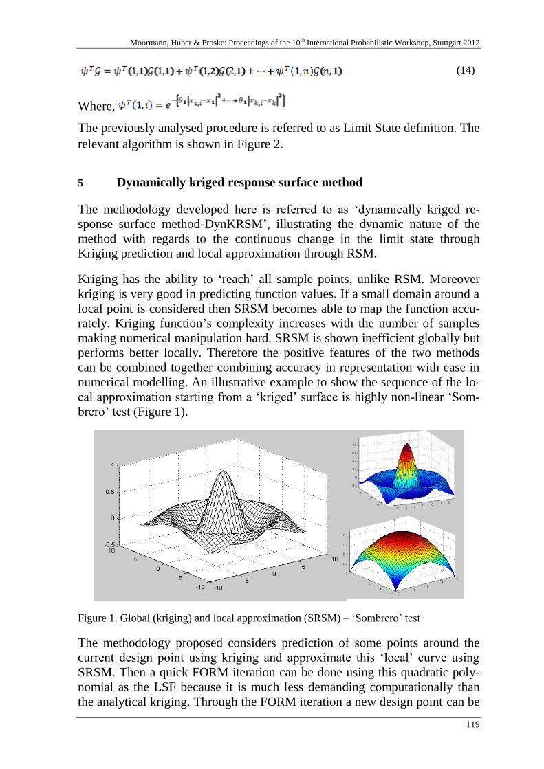
Moormann, Huber & Proske: Proceedings of the 10th International Probabilistic Workshop, Stuttgart 2012
119
(14)
Where,
The previously analysed procedure is referred to as Limit State definition. The
relevant algorithm is shown in Figure 2.
5 Dynamically kriged response surface method
The methodology developed here is referred to as ‘dynamically kriged re-
sponse surface method-DynKRSM’, illustrating the dynamic nature of the
method with regards to the continuous change in the limit state through
Kriging prediction and local approximation through RSM.
Kriging has the ability to ‘reach’ all sample points, unlike RSM. Moreover
kriging is very good in predicting function values. If a small domain around a
local point is considered then SRSM becomes able to map the function accu-
rately. Kriging function’s complexity increases with the number of samples
making numerical manipulation hard. SRSM is shown inefficient globally but
performs better locally. Therefore the positive features of the two methods
can be combined together combining accuracy in representation with ease in
numerical modelling. An illustrative example to show the sequence of the lo-
cal approximation starting from a ‘kriged’ surface is highly non-linear ‘Som-
brero’ test (Figure 1).
Figure 1. Global (kriging) and local approximation (SRSM) – ‘Sombrero’ test
The methodology proposed considers prediction of some points around the
current design point using kriging and approximate this ‘local’ curve using
SRSM. Then a quick FORM iteration can be done using this quadratic poly-
nomial as the LSF because it is much less demanding computationally than
the analytical kriging. Through the FORM iteration a new design point can be
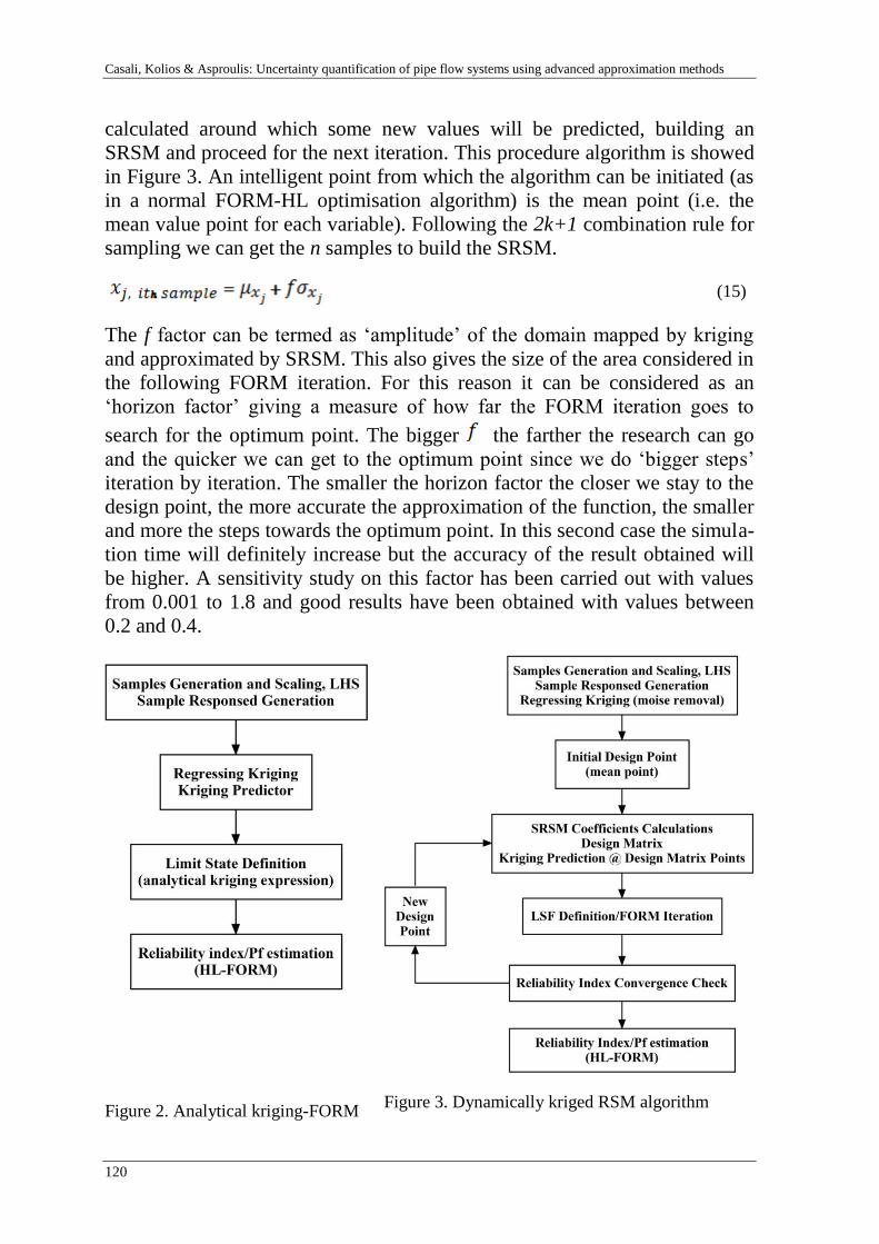
Casali, Kolios & Asproulis: Uncertainty quantification of pipe flow systems using advanced approximation methods
120
calculated around which some new values will be predicted, building an
SRSM and proceed for the next iteration. This procedure algorithm is showed
in Figure 3. An intelligent point from which the algorithm can be initiated (as
in a normal FORM-HL optimisation algorithm) is the mean point (i.e. the
mean value point for each variable). Following the 2k+1 combination rule for
sampling we can get the n samples to build the SRSM.
(15)
The f factor can be termed as ‘amplitude’ of the domain mapped by kriging
and approximated by SRSM. This also gives the size of the area considered in
the following FORM iteration. For this reason it can be considered as an
‘horizon factor’ giving a measure of how far the FORM iteration goes to
search for the optimum point. The bigger the farther the research can go
and the quicker we can get to the optimum point since we do ‘bigger steps’
iteration by iteration. The smaller the horizon factor the closer we stay to the
design point, the more accurate the approximation of the function, the smaller
and more the steps towards the optimum point. In this second case the simula-
tion time will definitely increase but the accuracy of the result obtained will
be higher. A sensitivity study on this factor has been carried out with values
from 0.001 to 1.8 and good results have been obtained with values between
0.2 and 0.4.
Figure 2. Analytical kriging-FORM Figure 3. Dynamically kriged RSM algorithm
Moormann, Huber & Proske: Proceedings of the 10th International Probabilistic Workshop, Stuttgart 2012
121
algorithm
6 Uncertainty of pipe flow systems
6.1 Description of the reference system
For the scope of this study, a system has been modelled initially deterministi-
cally using different tools for validation purposes: Matlab and Pipe Flow Ex-
pert 2010. Since both a global solution of the system (from differential
pressure to flow rate) and a partial solution (from flow rate and one pressure
to the missing one) are needed, two generic analytical models were devel-
oped. The models built in Matlab are based on well-known fluid mechanics
basic equations. Having a system, or a sub-system, delivering a flow from an
inlet node to an outlet node its geometry can be defined specifying the basic
quantities: length L, elevation h, diameter D, roughness ε, number and type of
bends and valves, component losses , pump characteristic, pressure,
flow rate and temperature. The elevation is considered positive if increasing
moving from the inlet node to the outlet node. The pipe roughness is depend-
ent from the material and can change during the system life introducing a
source of uncertainty. Bends and valves in a piping system have a significant
variability and building a code taking into account even half of them is first of
all useless and second of all too cumbersome. A free variable is introduced
where a total sum of all other component losses can be considered. A pump
characteristic can be defined with half a parabolic curve symmetrical to the y-
axis and concave downwards, hence only two coefficients are needed to de-
fine its behaviour (pump head vs. flow rate). No heat loss is considered from
the pipe (temperature constant). Table 1 presents the statistical properties of
the stochastic variables while Figure 4 illustrates the PID of the reference
flow system.
Table 1. Typical Coefficients of Variation
CoV Reference
Pressure 0.50% [8]
Temperature 0.20% [8]
Flow rate 0.50% [8]
Roughness 10.9% [23]
Level 0.5% [12]
Pump characteristic 10.1% [1]
Valve pressure drop 1.54% [22]

Casali, Kolios & Asproulis: Uncertainty quantification of pipe flow systems using advanced approximation methods
122
Figure 4. One phase-flow system
6.2 Limit states considered
For the safe and efficient operability of a pipe flow system all failure modes
need to be investigated. In this work 4 different scenarios exploring 3 failure
modes can be identified: maximum allowable pressure (in a pipe and in a
flange-gasket-flange, point A and B respectively), minimum efficiency allow-
able for the pump, minimum pressure difference for pressure-driven flow.
Limits for scenario 1A and 1B are taken from pipe characteristic catalogues
and set to 280,000 Pa and 200,000 Pa respectively, limit for pump efficiency
is set to 61% and the one for scenario 3 is set to the condition of having more
than atmospheric pressure at outlet point.
6.3 Simulation Results and Discussion
Figure 5 and 6 show the results from the techniques employed and developed.
As it can be shown, simple SRSM-FORM can estimate well the reliability
index in some of the scenarios but not for 1B where the probability of failure
is largely under-estimated. Focusing on this and trying to understand if the
low accuracy is introduced by SRSM or by FORM further analyses have been
carried out excluding those two techniques once at a time. Using SRSM-MCS
results are still insufficient but better than previously, implying that inaccura-
cy is due to SRSM. Performing analysis using kriging and MCS this trend can
be confirmed. Removing both SRSM and MCS from the analyses combining
kriging and FORM using the innovative and previously illustrated techniques
the results match the ones obtained through direct MCS.
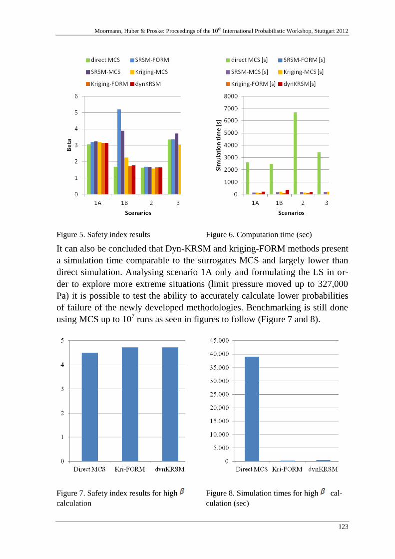
Moormann, Huber & Proske: Proceedings of the 10th International Probabilistic Workshop, Stuttgart 2012
123
Figure 5. Safety index results Figure 6. Computation time (sec)
It can also be concluded that Dyn-KRSM and kriging-FORM methods present
a simulation time comparable to the surrogates MCS and largely lower than
direct simulation. Analysing scenario 1A only and formulating the LS in or-
der to explore more extreme situations (limit pressure moved up to 327,000
Pa) it is possible to test the ability to accurately calculate lower probabilities
of failure of the newly developed methodologies. Benchmarking is still done
using MCS up to 107 runs as seen in figures to follow (Figure 7 and 8).
Figure 7. Safety index results for high
calculation
Figure 8. Simulation times for high cal-
culation (sec)
Casali, Kolios & Asproulis: Uncertainty quantification of pipe flow systems using advanced approximation methods
124
7 Conclusions
This paper has documented probabilistic assessment methods combining sto-
chastic response surface and surrogate modelling methods to MCS and
FORM methods for assessment of uncertainties. The methods developed ex-
tent current practice coupling kriging with FORM and suggesting a combina-
tion between kriging and SRSM in order to allow estimation of very low
probabilities of failure in relatively simple to model non-intrusive methods.
Application of the method in a typical single flow pipe system has shown that
the newly proposed methods perform very well both in aspects of accuracy
and in computation requirements. The same method has already been applied
by the authors for the case of a two phase flow system and highly non-linear
limit states with similarly good performance.
8 References
[1] ISO 9906:2012. Rotodynamic pumps - Hydraulic performance acceptance tests-
Grades 1( 2012), .
[2] Alfon, P., Soedarsono, J.W., Priadi, D. and Sulistijono, ( 2012), Pipeline material
reliability analysis regarding to probability of failure using corrosion degradation
model.
[3] Bai, Y., Moe, E. T. and Mork, K. (1994), "Probabilistic assessment of dented and
corroded pipeline", Proceedings of the International Offshore and Polar Engineering
Conference, Vol. 2, pp. 93.
[4] Bai, Y. and Referex (2001), Pipelines and risers, Elsevier, Amsterdam.
[5] Belov, D.A., Coupe, P., Fukuhara, M. and Myalo, E.V., ( 2011), Material-loss esti-
mation for pipes.
[6] Choi, S., Grandhi, R.V., Canfield, R.A. and SpringerLink, ( 2007), Reliability-based
structural design, Springer, London.
[7] Edwards, John, Mork, K., Norske, D. and Sydberger, T. (1996), "Reliability Based
Design of CO2 Corrosion Control", 24-29 March 1996, NACE International, .
[8] Elster Metering , available at: http://www.elster.com/en/index.
[9] Fleming, K. N. (2004), "Markov models for evaluating risk-informed in-service in-
spection strategies for nuclear power plant piping systems", Reliability Engineering &
System Safety, vol. 83, no. 1, pp. 27-45.

Moormann, Huber & Proske: Proceedings of the 10th International Probabilistic Workshop, Stuttgart 2012
125
[10] Forrester, A. I. J., Sóbester, A. and Keane, A. J. (2006), "Optimization with missing
data", Proceedings of the Royal Society A: Mathematical, Physical and Engineering
Sciences, vol. 462, no. 2067, pp. 935-945.
[11] Forrester, A.I.J., Sóbester, A. and Keane, A.J., ( 2008), Engineering design via sur-
rogate modelling, Wiley, Chichester, UK.
[12] Fulford, J. M., et al. (2006), Accuracy of radar water level measurements, available
at www.waterlog.com/media/pdfs/USGS-Study.pdf, accessed August 2012.
[13] Hasofer, A. M. and Lind, N. C. (1973), An exact and invariant First-Order Relia-
bility format, Solid Mechanic Division, University of Waterloo, Waterloo, Ontario,
Canada.
[14] Jeong, S., Yamamoto, K. and Obayashi, S. (2004), "Kriged-Based Probabilistic
Method for Constrained Multi-Objective Optimization Problem", AIAA Journal, , no.
6437.
[15] Jones, D. R. (2001), "A Taxonomy of Global Optimization Methods Based on Re-
sponse Surfaces", Journal of Global Optimization, vol. 21, no. 4, pp. 345-383.
[16] Khuri, A.I., ( 2001), An overview of the use of generalized linear models in re-
sponse surface methodology.
[17] Melchers, R. E. (1999), Structural reliability analysis and prediction, 2nd ed, John
Wiley, Chichester.
[18] Onoufriou, T. and Frangopol, D. M. (2002), "Reliability-based inspection optimiza-
tion of complex structures: a brief retrospective", Computers & Structures, vol. 80, no.
12, pp. 1133-1144.
[19] Proia, S. and Kolios, A. (2012), "Reliability assessment of complex structures in
composite materials under stochastic loading", World Journal of Mechanics, vol. 2,
pp. 162-170.
[20] Queipo, N. V., Haftka, R. T., Shyy, W., Goel, T., Vaidyanathan, R. and Kevin
Tucker, P. (2005), "Surrogate-based analysis and optimization", Progress in Aero-
space Sciences, vol. 41, no. 1, pp. 1-28.
[21] Quinio, A. and Kolios, A. (2010), "A stochastic finite element based approach to
the design optimization of a truss structure.", International Probabilistic Workshop,
The Netherlands, .
[22] Sandalci, M., Mançuhan, E., Alpman, E. and Küçükada, K. (2010), "Effect of the
flow conditions and valve size on butterfly valve performance", Isi Bilimi Ve Teknigi
Dergisi/ Journal of Thermal Science and Technology, vol. 30, no. 2, pp. 103-112.
[23] Wyant, J. C. and Creath, K. (1990), "Absolute measurement of surface roughness",
Proceedings of SPIE - The International Society for Optical Engineering, Vol. 1319,
pp. 568.

Casali, Kolios & Asproulis: Uncertainty quantification of pipe flow systems using advanced approximation methods
126
Moormann, Huber & Proske: Proceedings of the 10th International Probabilistic Workshop, Stuttgart 2012
127
Probability of corrosion detection with small
anodes
Sylvia Kessler, Christoph Gehlen
Centre for Building Materials, TU München, Germany
Abstract: For realistic and accurate description of the corrosion progress in re-
inforced concrete structures, the inspection results from detection of on-going
corrosion are of vital importance, in particular for the probabilistic service life
prediction. The crucial factor of the combination of inspection data and proba-
bilistic service life prediction is the knowledge about the accuracy of the meas-
urement method itself. The Probability of Detection (PoD) is a main descriptor
of the accuracy of qualitative inspection methods. Commonly, a PoD curve de-
scribes the rate of detecting a defect with given defect size s, PoD(s). In the
case of potential mapping, the defect size is the anode area. In this research, an
approach based on numerical models is pursued to obtain a PoD of potential
mapping for small anode areas. It is expected that through the integration of the
potential mapping data the condition of the structure and correspondingly the
service life time can be predicted more accurately.
1 Background
The corrosion of the reinforcement is often the major cause for the end of ser-
vice life of reinforced concrete structures. When cracks due to corrosion are
visible, the deterioration process is already advanced and cost intensive repair
is necessary. The only measurement method, which is able to distinguish non-
destructively between active or passive reinforcement before cracks occur, is
the potential mapping method. Figure 1 shows a modified Tuutti diagram
with the degree of deterioration due to corrosion in dependence of time.
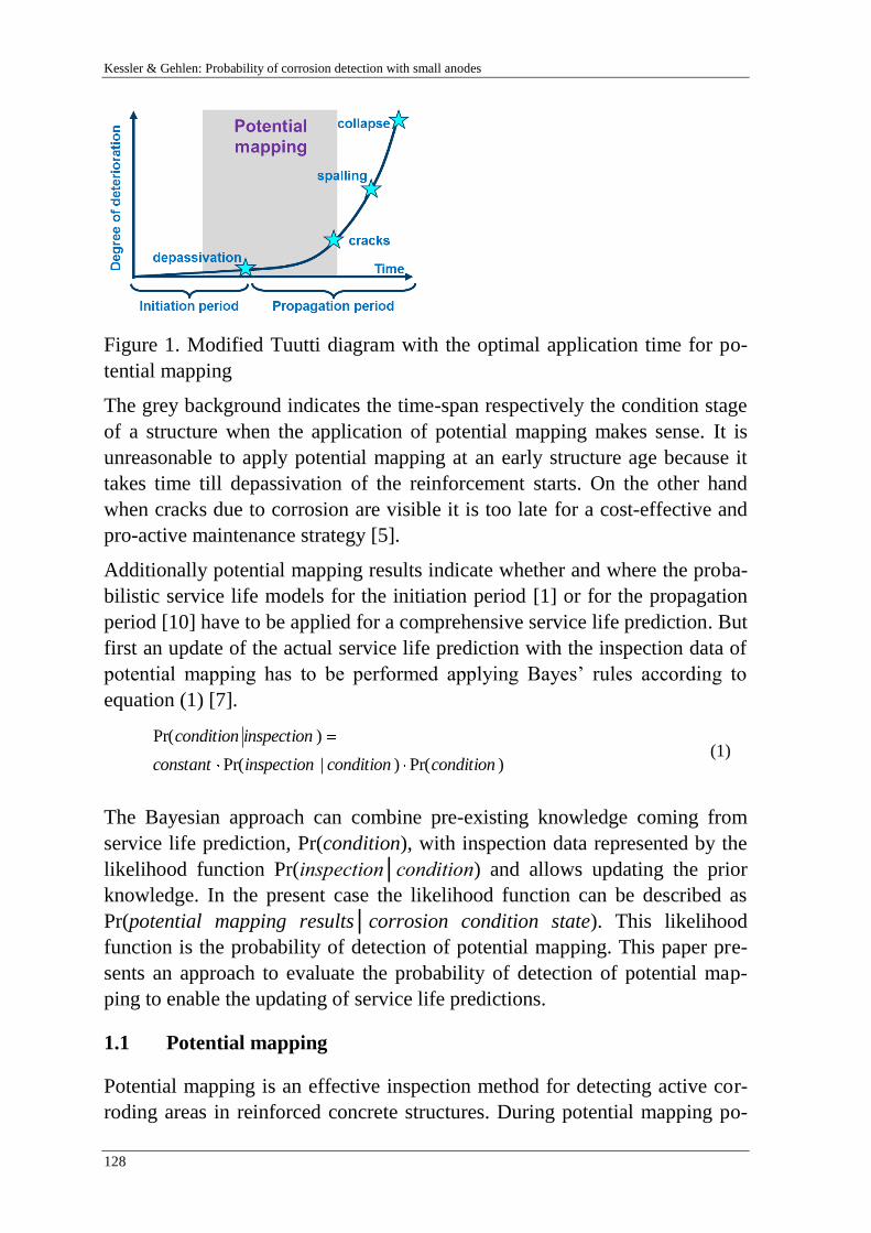
Kessler & Gehlen: Probability of corrosion detection with small anodes
128
Figure 1. Modified Tuutti diagram with the optimal application time for po-
tential mapping
The grey background indicates the time-span respectively the condition stage
of a structure when the application of potential mapping makes sense. It is
unreasonable to apply potential mapping at an early structure age because it
takes time till depassivation of the reinforcement starts. On the other hand
when cracks due to corrosion are visible it is too late for a cost-effective and
pro-active maintenance strategy [5].
Additionally potential mapping results indicate whether and where the proba-
bilistic service life models for the initiation period [1] or for the propagation
period [10] have to be applied for a comprehensive service life prediction. But
first an update of the actual service life prediction with the inspection data of
potential mapping has to be performed applying Bayes’ rules according to
equation (1) [7].
)Pr()|Pr(
)Pr(
conditionconditioninspectionconstant
inspectioncondition (1)
The Bayesian approach can combine pre-existing knowledge coming from
service life prediction, Pr(condition), with inspection data represented by the
likelihood function Pr(inspection│condition) and allows updating the prior
knowledge. In the present case the likelihood function can be described as
Pr(potential mapping results│corrosion condition state). This likelihood
function is the probability of detection of potential mapping. This paper pre-
sents an approach to evaluate the probability of detection of potential map-
ping to enable the updating of service life predictions.
1.1 Potential mapping
Potential mapping is an effective inspection method for detecting active cor-
roding areas in reinforced concrete structures. During potential mapping po-
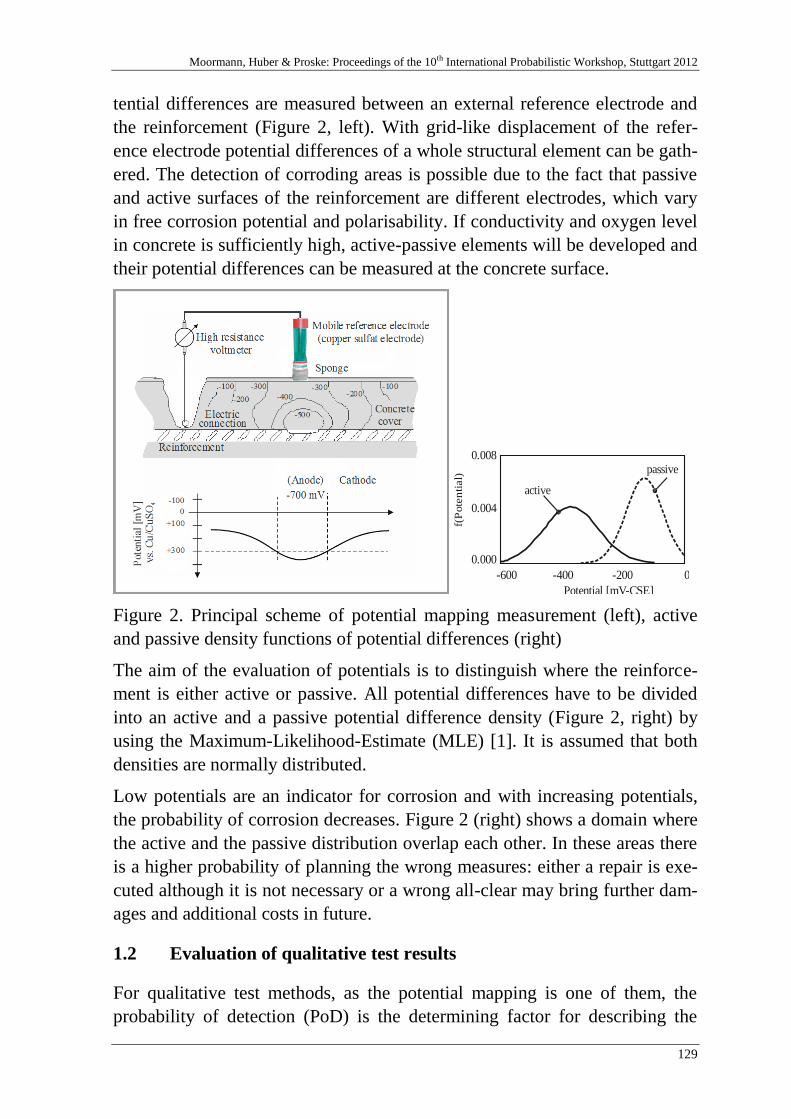
Moormann, Huber & Proske: Proceedings of the 10th International Probabilistic Workshop, Stuttgart 2012
129
tential differences are measured between an external reference electrode and
the reinforcement (Figure 2, left). With grid-like displacement of the refer-
ence electrode potential differences of a whole structural element can be gath-
ered. The detection of corroding areas is possible due to the fact that passive
and active surfaces of the reinforcement are different electrodes, which vary
in free corrosion potential and polarisability. If conductivity and oxygen level
in concrete is sufficiently high, active-passive elements will be developed and
their potential differences can be measured at the concrete surface.
active
passive
-600 -400 -200 0
0.000
0.004
0.008f(
Pote
nti
al)
Potential [mV-CSE]
Figure 2. Principal scheme of potential mapping measurement (left), active
and passive density functions of potential differences (right)
The aim of the evaluation of potentials is to distinguish where the reinforce-
ment is either active or passive. All potential differences have to be divided
into an active and a passive potential difference density (Figure 2, right) by
using the Maximum-Likelihood-Estimate (MLE) [1]. It is assumed that both
densities are normally distributed.
Low potentials are an indicator for corrosion and with increasing potentials,
the probability of corrosion decreases. Figure 2 (right) shows a domain where
the active and the passive distribution overlap each other. In these areas there
is a higher probability of planning the wrong measures: either a repair is exe-
cuted although it is not necessary or a wrong all-clear may bring further dam-
ages and additional costs in future.
1.2 Evaluation of qualitative test results
For qualitative test methods, as the potential mapping is one of them, the
probability of detection (PoD) is the determining factor for describing the
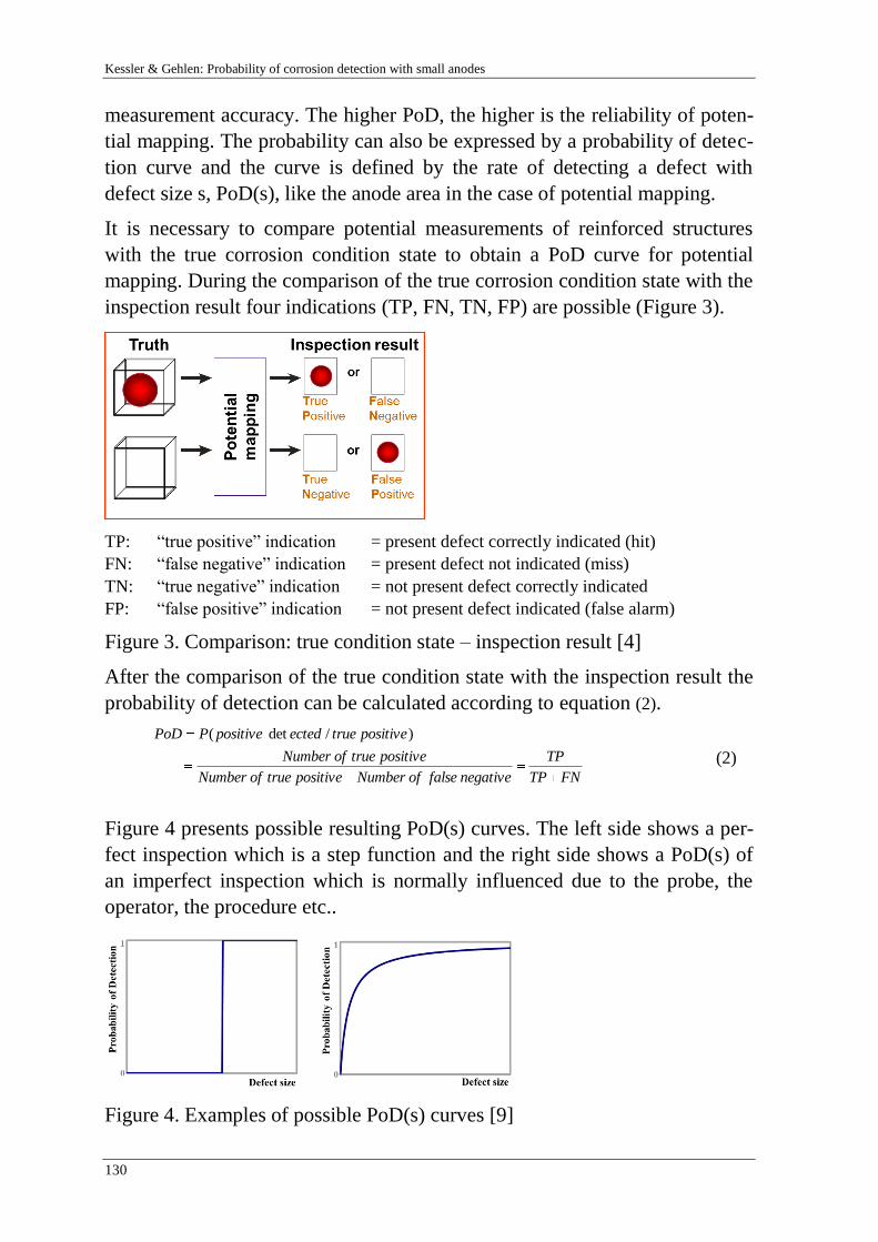
Kessler & Gehlen: Probability of corrosion detection with small anodes
130
measurement accuracy. The higher PoD, the higher is the reliability of poten-
tial mapping. The probability can also be expressed by a probability of detec-
tion curve and the curve is defined by the rate of detecting a defect with
defect size s, PoD(s), like the anode area in the case of potential mapping.
It is necessary to compare potential measurements of reinforced structures
with the true corrosion condition state to obtain a PoD curve for potential
mapping. During the comparison of the true corrosion condition state with the
inspection result four indications (TP, FN, TN, FP) are possible (Figure 3).
TP: “true positive” indication = present defect correctly indicated (hit)
FN: “false negative” indication = present defect not indicated (miss)
TN: “true negative” indication = not present defect correctly indicated
FP: “false positive” indication = not present defect indicated (false alarm)
Figure 3. Comparison: true condition state – inspection result [4]
After the comparison of the true condition state with the inspection result the
probability of detection can be calculated according to equation (2).
FNTP
TP
negativefalseofNumberpositivetrueofNumber
positivetrueofNumber
positivetrueectedpositivePPoD )/det( (2)
Figure 4 presents possible resulting PoD(s) curves. The left side shows a per-
fect inspection which is a step function and the right side shows a PoD(s) of
an imperfect inspection which is normally influenced due to the probe, the
operator, the procedure etc..
Figure 4. Examples of possible PoD(s) curves [9]

Moormann, Huber & Proske: Proceedings of the 10th International Probabilistic Workshop, Stuttgart 2012
131
The true corrosion condition state is only identifiable by replacement of con-
crete cover and visual inspection of the reinforcement. In general, owners will
not agree to open a whole structure for evaluating the accuracy of an inspec-
tion method. As a solution to this problem a numerical approach is used for
evaluating the PoD of potential mapping.
1.3 Numerical modelling of potential fields
Basically the corrosion processes inside an electrolyte and so the resulting
potential distributions are controlled by two different physical laws. The first
law is known as Ohms law (equation (3)). This law describes the flow of an
electrical charge in a medium as a result of a potential field. The current den-
sity is proportional to the gradient of the potential and inversely proportional
to the resistivity. The Laplace-equation (equation (4)) is the second law. This
equation calculates the propagation of the potentials field under steady-state
conditions.
Ohms law: 1
i
(3)
Laplace-equation for the electrolyte:
0 (4)
with Φ potential [V]
i
current density [A/m²]
ρ resistivity [Ωm] Anfang Namen.
The Laplace equation is a partial differential equation of second order. An
analytical solution for this equation can only be derived in case of certain ge-
ometries and boundary conditions. This is not possible for arbitrary geome-
tries; one has to use numerical means to calculate an appropriate
approximation [15].
The kinetics of the chemical reactions at the interface between concrete and
steel can be quantified by current density-polarization-curves (equation (5)).
)(fiN (5)
with iN current density [A/m²] Anfang Namen.
These curves describe how much current is produced or consumed at the steel
surface as a function of potential. These functions are usually non-linear and
represent the boundary conditions for the solution of the Laplace-equation.

Kessler & Gehlen: Probability of corrosion detection with small anodes
132
They can be obtained by experimental testing. Usually the polarization curves
are different for active and passive areas of the reinforcement.
The advantage of numerical simulation is that the corrosion condition of nu-
merical models can be varied. The presented numerical calculations are real-
ized with the Boundary Element Method software BEASY [17]. This
simulation software is validated in [6], [8] and [13].
2 Probability of detection of potential mapping
2.1 Numerical model
One of the most important chloride exposed construction component is a rein-
forced concrete plate like a bridge deck or a garage ceiling. Therefore it was
decided to model the probability of detection of a plate first. That’s why the
numerical model is comparable to a section of a reinforced concrete plate.
The dimension of the numerical model has to be bigger than the expansion of
the macro cell element of the corrosion process. This condition is fulfilled
when no corrosion current takes place at the model boundary. Otherwise the
modelled corrosion process would be limited by a lack of cathodic areas and
this case isn’t realistic for plates.
The expansion of the macro cell element is approximately 1.0 m according to
Warkus [13]. The anode area is located at the centre of the model. So taking
into account the expansion of the macro cell element the quadratic numerical
model has a side length of 2 m. The model contains four reinforcement layers
with a diameter of 10 mm and a rod distance of 20 cm. Figure 5 shows the
numerical model.
Figure 5. Numerical model of the section of a reinforced concrete plate (left),
with elements (right)
It is modelled only a quarter of the plate to take the advantage of the model
symmetry. Figure 6 presents a typical result of a numerically simulated poten-
tial field.
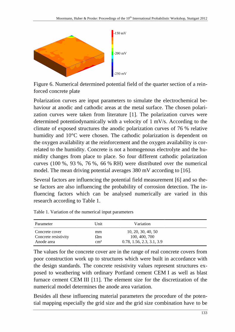
Moormann, Huber & Proske: Proceedings of the 10th International Probabilistic Workshop, Stuttgart 2012
133
Figure 6. Numerical determined potential field of the quarter section of a rein-
forced concrete plate
Polarization curves are input parameters to simulate the electrochemical be-
haviour at anodic and cathodic areas at the metal surface. The chosen polari-
zation curves were taken from literature [1]. The polarization curves were
determined potentiodynamically with a velocity of 1 mV/s. According to the
climate of exposed structures the anodic polarization curves of 76 % relative
humidity and 10°C were chosen. The cathodic polarization is dependent on
the oxygen availability at the reinforcement and the oxygen availability is cor-
related to the humidity. Concrete is not a homogenous electrolyte and the hu-
midity changes from place to place. So four different cathodic polarization
curves (100 %, 93 %, 76 %, 66 % RH) were distributed over the numerical
model. The mean driving potential averages 380 mV according to [16].
Several factors are influencing the potential field measurement [6] and so the-
se factors are also influencing the probability of corrosion detection. The in-
fluencing factors which can be analysed numerically are varied in this
research according to Table 1.
Table 1. Variation of the numerical input parameters
Parameter Unit Variation
Concrete cover
Concrete resistivity
Anode area
mm
Ωm
cm²
10, 20, 30, 40, 50
100, 400, 700
0.78, 1.56, 2.3, 3.1, 3.9
The values for the concrete cover are in the range of real concrete covers from
poor construction work up to structures which were built in accordance with
the design standards. The concrete resistivity values represent structures ex-
posed to weathering with ordinary Portland cement CEM I as well as blast
furnace cement CEM III [11]. The element size for the discretization of the
numerical model determines the anode area variation.
Besides all these influencing material parameters the procedure of the poten-
tial mapping especially the grid size and the grid size combination have to be
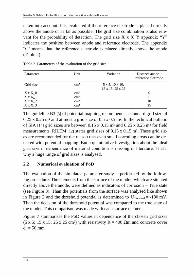
Kessler & Gehlen: Probability of corrosion detection with small anodes
134
taken into account. It is evaluated if the reference electrode is placed directly
above the anode or as far as possible. The grid size combination is also rele-
vant for the probability of detection. The grid size X x X_Y appendix “Y”
indicates the position between anode and reference electrode. The appendix
“0” means that the reference electrode is placed directly above the anode
(Table 2).
Table 2. Parameters of the evaluation of the grid size
Parameter Unit Variation Distance anode –
reference electrode
Grid size
X x X_0
X x X_1
X x X_2
X x X_3
cm²
cm²
cm²
cm²
cm²
5 x 5; 10 x 10;
15 x 15; 25 x 25
0
5
10
15
The guideline B3 [3] of potential mapping recommends a standard grid size of
0.25 x 0.25 m² and at most a grid size of 0.5 x 0.5 m². In the technical bulletin
of SIA [14] grid sizes are between 0.15 x 0.15 m² and 0.25 x 0.25 m² for field
measurements. RILEM [12] states grid sizes of 0.15 x 0.15 m². These grid siz-
es are recommended for the reason that even small corroding areas can be de-
tected with potential mapping. But a quantitative investigation about the ideal
grid size in dependence of material condition is missing in literature. That’s
why a huge range of grid sizes is analysed.
2.2 Numerical evaluation of PoD
The evaluation of the simulated parameter study is performed by the follow-
ing procedure. The elements from the surface of the model, which are situated
directly above the anode, were defined as indicators of corrosion – True state
(see Figure 3). Than the potentials from the surface was analysed like shown
in Figure 2 and the threshold potential is determined to Uthreshold = -180 mV.
Than the decision of the threshold potential was compared to the true state of
the model. This comparison was made with each surface element.
Figure 7 summarises the PoD values in dependence of the chosen grid sizes
(5 x 5; 15 x 15; 25 x 25 cm²) with resistivity R = 400 Ωm and concrete cover
dc = 50 mm.
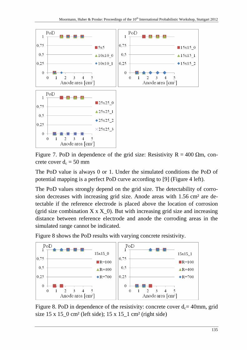
Moormann, Huber & Proske: Proceedings of the 10th International Probabilistic Workshop, Stuttgart 2012
135
Figure 7. PoD in dependence of the grid size: Resistivity R = 400 Ωm, con-
crete cover dc = 50 mm
The PoD value is always 0 or 1. Under the simulated conditions the PoD of
potential mapping is a perfect PoD curve according to [9] (Figure 4 left).
The PoD values strongly depend on the grid size. The detectability of corro-
sion decreases with increasing grid size. Anode areas with 1.56 cm² are de-
tectable if the reference electrode is placed above the location of corrosion
(grid size combination X x X_0). But with increasing grid size and increasing
distance between reference electrode and anode the corroding areas in the
simulated range cannot be indicated.
Figure 8 shows the PoD results with varying concrete resistivity.
Figure 8. PoD in dependence of the resistivity: concrete cover dc= 40mm, grid
size 15 x 15_0 cm² (left side); 15 x 15_1 cm² (right side)
15x15_0 15x15_1
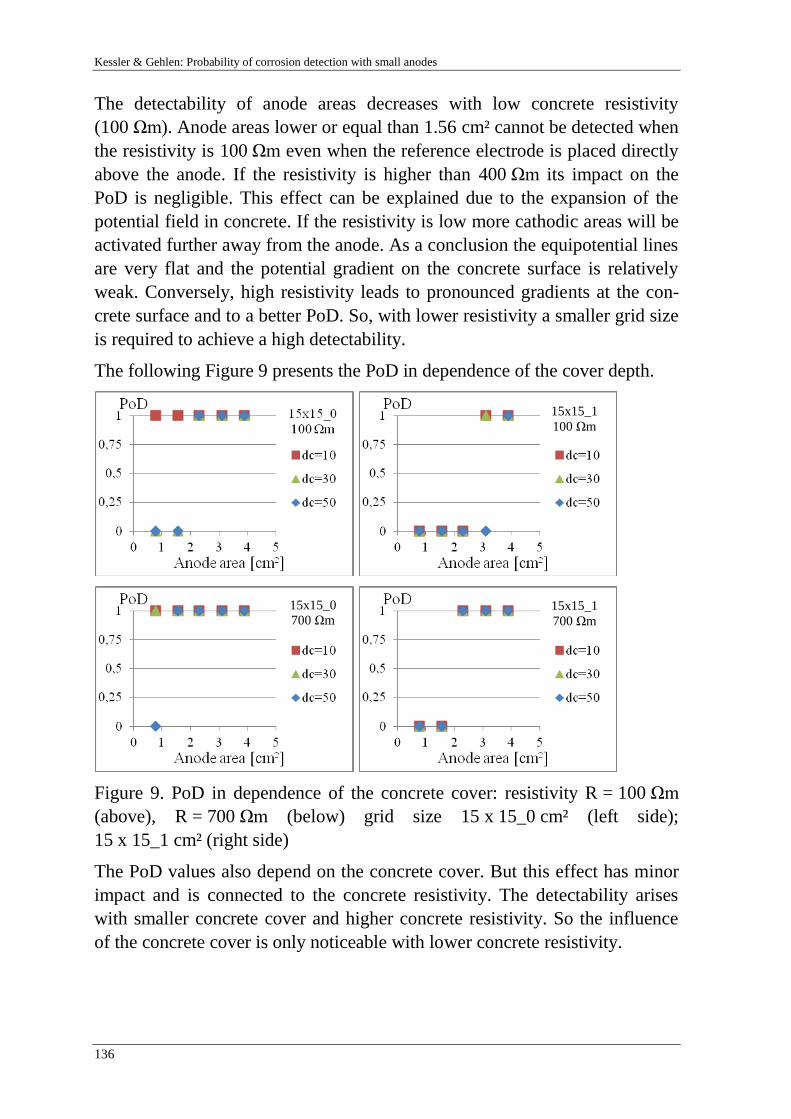
Kessler & Gehlen: Probability of corrosion detection with small anodes
136
The detectability of anode areas decreases with low concrete resistivity
(100 Ωm). Anode areas lower or equal than 1.56 cm² cannot be detected when
the resistivity is 100 Ωm even when the reference electrode is placed directly
above the anode. If the resistivity is higher than 400 Ωm its impact on the
PoD is negligible. This effect can be explained due to the expansion of the
potential field in concrete. If the resistivity is low more cathodic areas will be
activated further away from the anode. As a conclusion the equipotential lines
are very flat and the potential gradient on the concrete surface is relatively
weak. Conversely, high resistivity leads to pronounced gradients at the con-
crete surface and to a better PoD. So, with lower resistivity a smaller grid size
is required to achieve a high detectability.
The following Figure 9 presents the PoD in dependence of the cover depth.
Figure 9. PoD in dependence of the concrete cover: resistivity R = 100 Ωm
(above), R = 700 Ωm (below) grid size 15 x 15_0 cm² (left side);
15 x 15_1 cm² (right side)
The PoD values also depend on the concrete cover. But this effect has minor
impact and is connected to the concrete resistivity. The detectability arises
with smaller concrete cover and higher concrete resistivity. So the influence
of the concrete cover is only noticeable with lower concrete resistivity.
15x15_1 100 Ωm
15x15_0 700 Ωm
15x15_1 700 Ωm
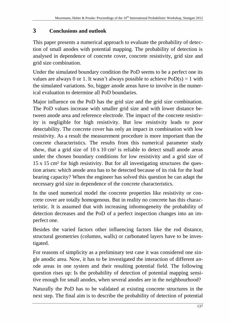
Moormann, Huber & Proske: Proceedings of the 10th International Probabilistic Workshop, Stuttgart 2012
137
3 Conclusions and outlook
This paper presents a numerical approach to evaluate the probability of detec-
tion of small anodes with potential mapping. The probability of detection is
analysed in dependence of concrete cover, concrete resistivity, grid size and
grid size combination.
Under the simulated boundary condition the PoD seems to be a perfect one its
values are always 0 or 1. It wasn’t always possible to achieve PoD(s) = 1 with
the simulated variations. So, bigger anode areas have to involve in the numer-
ical evaluation to determine all PoD boundaries.
Major influence on the PoD has the grid size and the grid size combination.
The PoD values increase with smaller grid size and with lower distance be-
tween anode area and reference electrode. The impact of the concrete resistiv-
ity is negligible for high resistivity. But low resistivity leads to poor
detectability. The concrete cover has only an impact in combination with low
resistivity. As a result the measurement procedure is more important than the
concrete characteristics. The results from this numerical parameter study
show, that a grid size of 10 x 10 cm² is reliable to detect small anode areas
under the chosen boundary conditions for low resistivity and a grid size of
15 x 15 cm² for high resistivity. But for all investigating structures the ques-
tion arises: which anode area has to be detected because of its risk for the load
bearing capacity? When the engineer has solved this question he can adapt the
necessary grid size in dependence of the concrete characteristics.
In the used numerical model the concrete properties like resistivity or con-
crete cover are totally homogenous. But in reality no concrete has this charac-
teristic. It is assumed that with increasing inhomogeneity the probability of
detection decreases and the PoD of a perfect inspection changes into an im-
perfect one.
Besides the varied factors other influencing factors like the rod distance,
structural geometries (columns, walls) or carbonated layers have to be inves-
tigated.
For reasons of simplicity as a preliminary test case it was considered one sin-
gle anodic area. Now, it has to be investigated the interaction of different an-
ode areas in one system and their resulting potential field. The following
question rises up: Is the probability of detection of potential mapping sensi-
tive enough for small anodes, when several anodes are in the neighbourhood?
Naturally the PoD has to be validated at existing concrete structures in the
next step. The final aim is to describe the probability of detection of potential
Kessler & Gehlen: Probability of corrosion detection with small anodes
138
mapping mathematically in dependence of their most influencing parameters.
When this aim is achieved it simplifies the updating of service life prediction
with potential mapping data.
4 References
[1] Brem, M. (2004) Numerische Simulation der Korrosion in Stahlbetonbauteilen, Diss.
ETH Nr. 15567, Zürich
[2] Ditlevsen, O.: Uncertainty modeling: With applications to multidimensional civil
engineering systems. New York: McGraw-Hill, 1981. – ISBN 0-07-017046-0
[3] DGZfP Merkblatt B3 2008 Elektrochemische Potentialmessungen zur Detektion von
Bewehrungsstahlkorrosion (in German)
[4] Gehlen, C.: Probabilistische Lebensdauerbemessung von Stahlbetonbauwerken –
Zuverlässigkeitsbetrachtungen zur wirksamen Vermeidung von Bewehrungskorrosi-
on Dissertation, RWTH Aachen (in German), 2001
[5] Gehlen, C. et al.: Condition Control and Assessment of Reinforced Concrete Struc-
tures Exposed to Corrosive Environments (Carbonation / Chlorides), fib bulletin 59,
2011
[6] Keßler, S.; Ebell, G.; Gehlen, C.; Burkert, A.: Die Aussagegenauigkeit der Potential-
feldmessung, In, Beton- und Stahlbetonbau Volume 106, Issue 7, p. 481–489, 2011
(German)
[7] Keßler, S; Fischer, J.; Straub, D.; Gehlen, C.: Updating of service life prediction of
reinforced concrete structures with potential mapping, ICDC, International confer-
ence on durability of concrete, Trondheim Norway June 18-21, 2012
[8] Kessler, S.; Gehlen, C. (2010) Potential mapping – Possibilities and limits 8th fib
PhD Symposium in Kgs. Lyngby, Denmark
[9] MIL-HDBK-1823A, Department of Defense Handbook, Nondestructive Evaluation
System Reliability Assessment, 7. April 2009
[10] Osterminski, K.; Schießl, P.: Design model for reinforcement corrosion. Structural
Concrete, Vol. 13, No. 3, 2012.
[11] Osterminski, K., Tian, W., Schießl, P., Gehlen, C.: Elektrolytwiderstand von Beton
und Korrosion in gerissenem Beton. In: „Dauerhaftigkeitsbemessung von Stahlbe-
tonbauteilen auf Bewehrungskorrosion – Teil 1: Systemparameter der Bewehrungs-
korrosion“ Schriftenreihe des Deutschen Ausschusses für Stahlbeton e. V., Heft 601,
Beuth Verlag, Berlin, 2012 (German).
[12] RILEM Technical Committees Elsener, B. Andrade, C. Gulikers, J. Polder R. and
Raupach, M. 2003 Half-cell potential measurements – potential mapping on rein-
forced concrete structures. Materials and Structures, 36: 461–471

Moormann, Huber & Proske: Proceedings of the 10th International Probabilistic Workshop, Stuttgart 2012
139
[13] Schießl, P., Osterminski, K., Isecke, B., Beck, M., Burkert, A., Raupach, M.,
Harnisch, J., Warkus, J., Tian, W.: Deterioration model and input parameters for re-
inforcement corrosion. Structural Concrete, Vol. 13, No. 3, 2012.
[14] SIA 2006 Durchführung und Interpretation der Potentialfeldmessung an Stahlbeton-
bauteilen Zürich (in German)
[15] Warkus, J.; Raupach, M.; Gulikers, J. (2006), Numerical modeling of corrosion –
Theoretical backgrounds - Materials and Corrosion, 57, No. 8
[16] Warkus, J. Raupach, M. (2009) Modelling of reinforcement corrosion – geometrical
effects on macrocell corrosion, Materials and Corrosion, 61, Issue 6, p. 494–504
[17] www.beasy.com

Kessler & Gehlen: Probability of corrosion detection with small anodes
140

Moormann, Huber & Proske: Proceedings of the 10th International Probabilistic Workshop, Stuttgart 2012
141
Investigation of Reliability Model for Cracking in
South African Reinforced Concrete Water
Retaining Structures
C.H. McLeod, J.A. Wium, J.V. Retief
University of KwaZulu-Natal, Durban & University of Stellenbosch, Cape Town,
South Africa
Abstract: The development of a design code of practice for concrete water retaining
structures (WRS) in South African is presently underway, along with the revision of
the code of practice for reinforced concrete structures (SANS 10100). This paper
discusses part of the research undertaken in the development of the new design code
for WRS, namely, the serviceability limit state of cracking due to loads and/or
restrained deformations. The basic crack model considered here is that utilized by
Eurocode EN1992-1-1 (2004) and EN1992-3 (2006) which predicts the maximum
crack width using a basic compatibility relationship between strain and cracking.
This crack width is then compared to a limiting crack width value. A reliability
model for load-induced cracking is presented in this paper using the EN1992 crack
model applied to South African conditions. The influence of the variables, including
model uncertainty on the reliability of the crack model is investigated.
1. Introduction
This paper presents a portion of the research carried out in the development of a
South African design standard for water retaining structures (WRS). South African
designers currently use the British codes in the design of reinforced concrete
water-retaining structures (WRS) as a South African design code for WRS does
not exist at present.
As the serviceability limit state (SLS) of cracking tends to be dominant in the
design of WRS, with failure to meet this limit state resulting in a loss of function of
the structure, a reliability model was developed to assess the EN1992 crack model
[5] for cracking due to loading effects applied to South African conditions, using

McLeod, Wium & Retief: Investigation of reliability model for cracking in South African reinforced concrete water retaining
structures
142
the First Order Reliability Method (FORM). This paper presents the investigation
of the parameters of the reliability model for cracking in reinforced concrete. Two
cases of load-induced cracking were considered, namely, those due to pure tension
and pure bending. SANS10160-2011[12] was referred to in determining the loads
and serviceability reliability levels for the crack model, with SANS10100-
2000[10] used as the basis for the material properties used in the model. The
reliability crack models were set up and analysed using Microsoft EXCEL.
2. Development of reliability models for tension and flexural cracking
Limiting crack width
The current practice in designing WRS for SLS cracking in South Africa using
BS8007 [3] is to specify a limiting crack width of 0,2 mm. A limit of 0,1 mm may
also be used, for aesthetic concerns. EN1992-3[6] specifies limits from 0,2 mm to
0,05mm depending on the hydrostatic ratio of depth of water to wall thickness
(hD/h) for cracks passing through the section and where the existence of a
compression zone cannot be guaranteed. Therefore the results of reliability
analyses with crack widths of 0,2 mm, 0,1 mm and 0,05mm are presented here.
Structural configuration of models for tension and flexural cracking
Representative structural models were used for both serviceability pure tension and
flexural cracking in a WRS. The load case considered was for a permanent load
due to hydrostatic pressure to SANS10160-2011 [12].
2.2.1 Example of pure flexure in a WRS
For the flexural case, consider a 1 m section of wall of a rectangular reinforced
concrete water-retaining structure, designed as a vertical cantilever. The wall is
subject to flexure about a vertical axis due to water pressure. The maximum liquid
load is Lk = H. γw where γw is 9,81 kN/m3. The wall height (H) was taken as 5m
and 7m, resulting in water pressures of 49,1 and 68,7 kN/m2 per m of wall and
corresponding maximum bending moments of 204,6 and 401,0 kNm.
2.2.2 Example of pure tension in a WRS
For the tension case, a 1 m section of wall in a circular reservoir is considered. The

Moormann, Huber & Proske: Proceedings of the 10th International Probabilistic Workshop, Stuttgart 2012
143
wall is subject to hoop tension due to water pressure (Lk) in the horizontal plane. A
reservoir diameter of 28 m is selected. The maximum nominal tensile forces of
686,7kN and 961,4 kN for wall heights of 5 m and 7 m, respectively, is obtained.
Development of limit state equation for reliability crack model
The first step in setting up the reliability model for cracking using FORM was to
define the limit state (LS) equation. The SLS criterion for cracking will be met if
the calculated crack width is less than the specified crack width limit. Thus the LS
equation is:
g = wlim – θ.wm (1)
where wlim is the limiting crack width, θ is model uncertainty and wm is the crack
width. The crack width, wm, is determined from the basic compatibility equation,
wm = Srm . εm (2)
where Srm is crack spacing and εm is average strain.
The crack spacing Srm is determined from the equation developed for EN1992, as
described by BEEBY et al [1]:
Srm = 2c + 0,25k1k2φ /ρp,eff (3)
where c is concrete cover, k1is a coefficient for high tensile reinforcement bond, k2
is a coefficient for stress distribution, φ is bar diameter and ρp,eff is the effective
reinforcement ratio.
The average strain for reinforced concrete as given by EN1992 [5] is:
where εsm is steel strain, εcm is concrete strain, σs is steel stress, Es is the steel
modulus of elasticity, kt is a coefficient for duration of loading, fct,eff is effective
concrete tensile strength and αe is the modular ratio, Es/Ec,eff. The modular ratio,
αe, is the ratio Es/Ec where Ec is the effective concrete modulus. The effective
reinforcement ratio is defined as:
ρp, eff = As/ Act,eff = As/( b.hc,eff) (5)
where As tension reinforcement area, Act,eff is the effective area of concrete in
tension, b is the cross sectional width and hc,eff is the effective depth of concrete in
tension.
McLeod, Wium & Retief: Investigation of reliability model for cracking in South African reinforced concrete water retaining
structures
144
The effective depth of concrete in tension, hc, eff, as defined by EN1992 [5], is the
lesser of either (h – x)/3, h/2 or 2,5(h - d). In the flexural cracking case, (h – x)/3
was found to be limiting, while in the tension cracking case, the limiting equation
was dependent on the combination of section thickness (h), concrete cover (c) and
bar diameter (φ), being either h/2 or 2,5 (c + φ/2). Thus, as the former equation is
in terms of the basic variable section thickness only and the latter in terms of the
basic variable cover (and independent of section thickness), two reliability models
were set up for tension cracking.
The equations (1) to (5) are expressed in terms of the basic random variables of
section thickness (h), concrete cover (c), liquid load (Lk) and concrete tensile
strength (fct,eff ).
2.4 Parameters of the reliability crack model
Typical values used for the parameters of the reliability model were obtained from
current industry practices in South Africa [13]. Statistical data was obtained from
sources such as the JOINT COMMITTEE FOR STRUCTURAL SAFETY [8] and
HOLICKY [7]. Table 1 summarises the statistical data used for all parameters in the
reliability models for tension and flexural cracking. The reinforcement area (as a
deterministic value) was used as the basis for comparison.
The database for model uncertainty with regard to concrete cracking is very small,
so some assumptions were made based on the available information. A general
value used for the model uncertainty coefficient of variation (CoV) is 0,1 in
structural reliability models, as used by HOLICKY [7], and was taken to be the
lower limit and the reference level. A maximum value of 0,3 has been suggested in
research as being appropriate to cracking in reinforced concrete beams by QUAN et
al [9] and was therefore considered here to be the maximum limit. To investigate
the effect of model uncertainty variation on the cracking models, reliability
analyses were performed for a range of values for the CoV from 0,1 to 0,3.
Level of Reliability, β
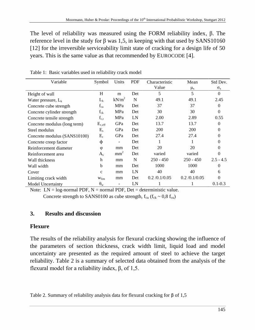
Moormann, Huber & Proske: Proceedings of the 10th International Probabilistic Workshop, Stuttgart 2012
145
The level of reliability was measured using the FORM reliability index, β. The
reference level in the study for β was 1,5, in keeping with that used by SANS10160
[12] for the irreversible serviceability limit state of cracking for a design life of 50
years. This is the same value as that recommended by EUROCODE [4].
Table 1: Basic variables used in reliability crack model
Variable
Symbol
Units
Characteristic Value
Mean μx
Std Dev. σx
Height of wall H m Det 5 5 0
Water pressure, Lk Lk kN/m2 N 49.1 49.1 2.45
Concrete cube strength fcu MPa Det 37 37 0
Concrete cylinder strength fck MPa Det 30 30 0
Concrete tensile strength fc,t MPa LN 2.00 2.89 0.55
Concrete modulus (long term) Ec,eff GPa Det 13.7 13.7 0
Steel modulus Es GPa Det 200 200 0
Concrete modulus (SANS10100) Ec GPa Det 27.4 27.4 0
Concrete creep factor ϕ - Det 1 1 0
Reinforcement diameter φ mm Det 20 20 0
Reinforcement area As mm2 Det varied varied 0
Wall thickness h mm N 250 - 450 250 - 450 2.5 - 4.5
Wall width b mm Det 1000 1000 0
Cover c mm LN 40 40 6
Limiting crack width wlim mm Det 0.2 /0.1/0.05 0.2 /0.1/0.05 0
Model Uncertainty θw - LN 1 1 0.1-0.3
Note: LN = log-normal PDF, N = normal PDF, Det = deterministic value.
Concrete strength to SANS0100 as cube strength, fcu (fck ~ 0,8 fcu)
3. Results and discussion
Flexure
The results of the reliability analysis for flexural cracking showing the influence of
the parameters of section thickness, crack width limit, liquid load and model
uncertainty are presented as the required amount of steel to achieve the target
reliability. Table 2 is a summary of selected data obtained from the analysis of the
flexural model for a reliability index, β, of 1,5.
Table 2. Summary of reliability analysis data for flexural cracking for β of 1,5
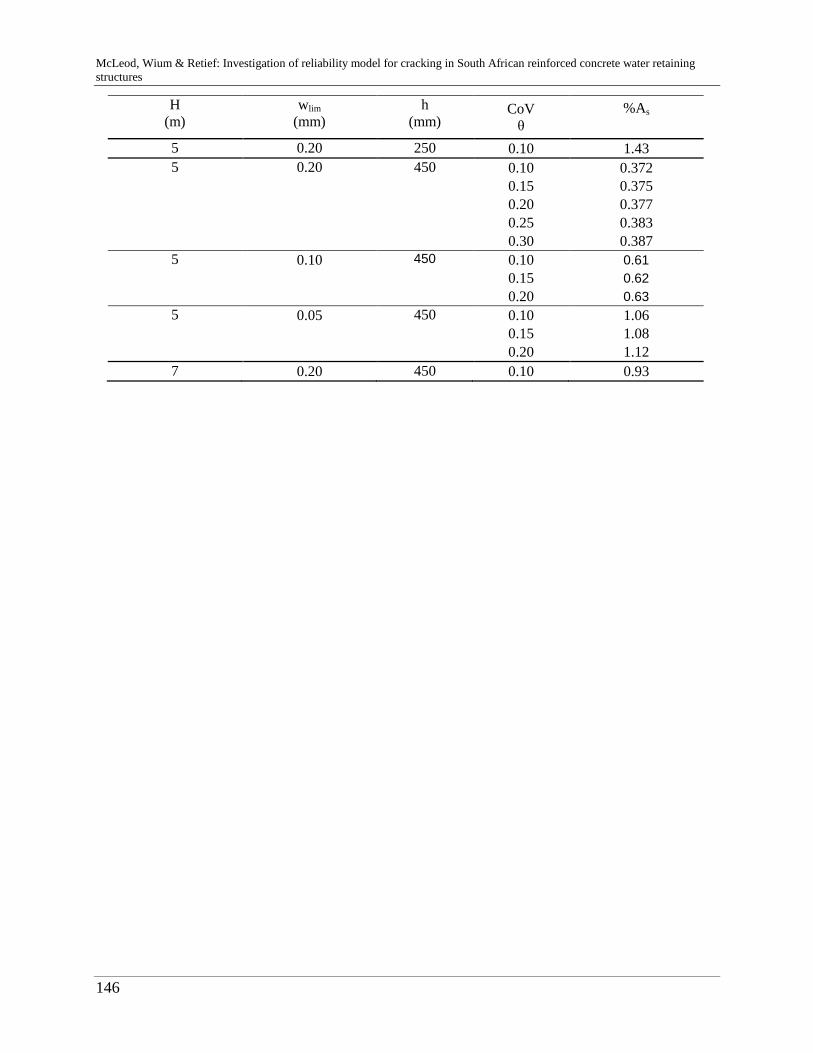
McLeod, Wium & Retief: Investigation of reliability model for cracking in South African reinforced concrete water retaining
structures
146
H (m)
wlim
(mm) h
(mm) CoV
θ %As
5 0.20 250 0.10 1.43
5 0.20 450 0.10 0.372
0.15 0.375
0.20 0.377
0.25 0.383
0.30 0.387
5 0.10 450 0.10 0.61
0.15 0.62
0.20 0.63
5 0.05 450 0.10 1.06
0.15 1.08
0.20 1.12
7 0.20 450 0.10 0.93
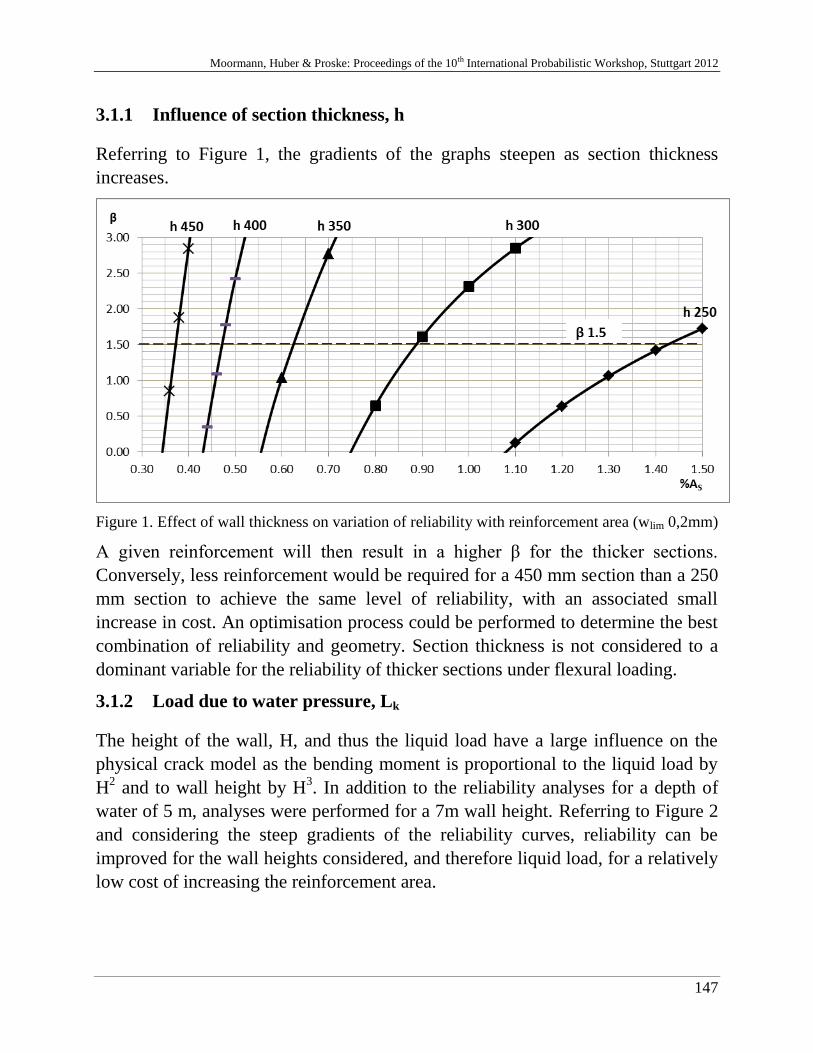
Moormann, Huber & Proske: Proceedings of the 10th International Probabilistic Workshop, Stuttgart 2012
147
3.1.1 Influence of section thickness, h
Referring to Figure 1, the gradients of the graphs steepen as section thickness
increases.
Figure 1. Effect of wall thickness on variation of reliability with reinforcement area (wlim 0,2mm)
A given reinforcement will then result in a higher β for the thicker sections.
Conversely, less reinforcement would be required for a 450 mm section than a 250
mm section to achieve the same level of reliability, with an associated small
increase in cost. An optimisation process could be performed to determine the best
combination of reliability and geometry. Section thickness is not considered to a
dominant variable for the reliability of thicker sections under flexural loading.
3.1.2 Load due to water pressure, Lk
The height of the wall, H, and thus the liquid load have a large influence on the
physical crack model as the bending moment is proportional to the liquid load by
H2 and to wall height by H
3. In addition to the reliability analyses for a depth of
water of 5 m, analyses were performed for a 7m wall height. Referring to Figure 2
and considering the steep gradients of the reliability curves, reliability can be
improved for the wall heights considered, and therefore liquid load, for a relatively
low cost of increasing the reinforcement area.
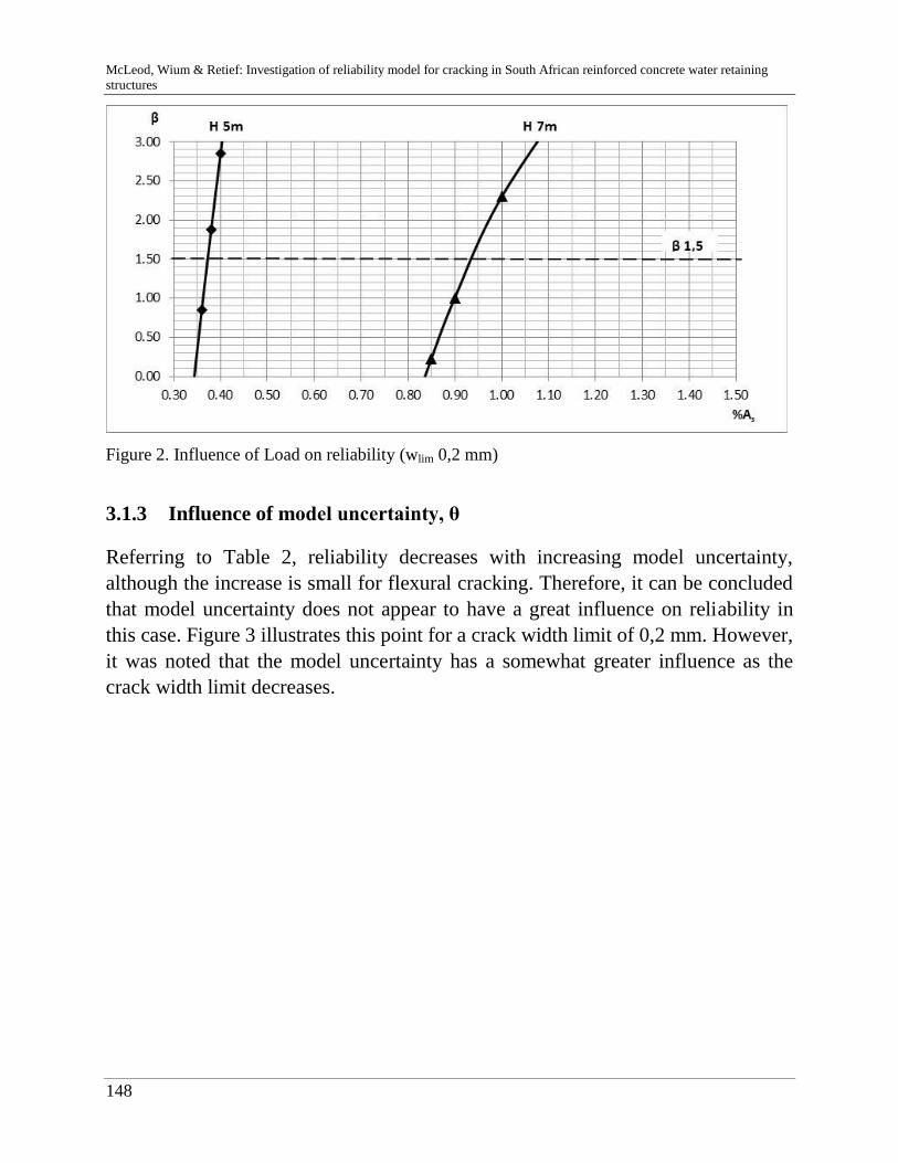
McLeod, Wium & Retief: Investigation of reliability model for cracking in South African reinforced concrete water retaining
structures
148
Figure 2. Influence of Load on reliability (wlim 0,2 mm)
3.1.3 Influence of model uncertainty, θ
Referring to Table 2, reliability decreases with increasing model uncertainty,
although the increase is small for flexural cracking. Therefore, it can be concluded
that model uncertainty does not appear to have a great influence on reliability in
this case. Figure 3 illustrates this point for a crack width limit of 0,2 mm. However,
it was noted that the model uncertainty has a somewhat greater influence as the
crack width limit decreases.
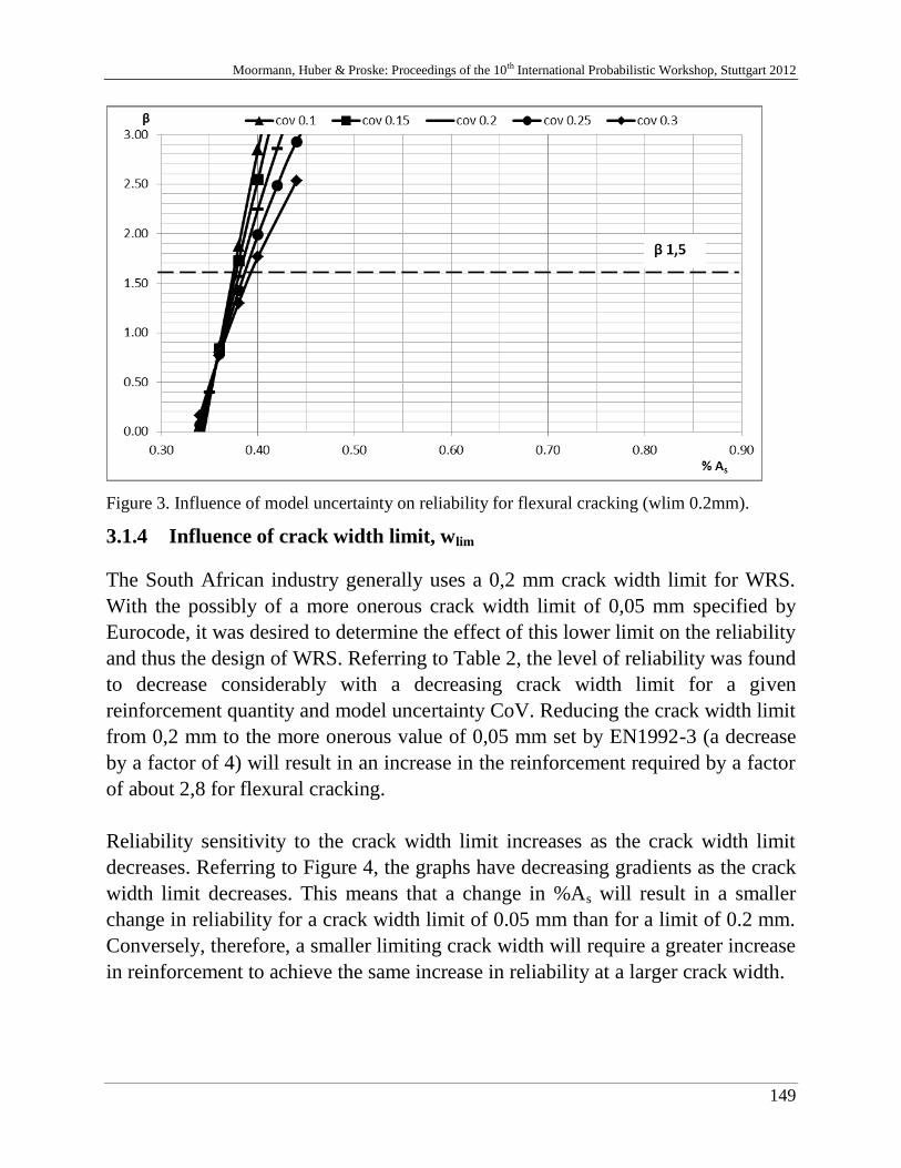
Moormann, Huber & Proske: Proceedings of the 10th International Probabilistic Workshop, Stuttgart 2012
149
Figure 3. Influence of model uncertainty on reliability for flexural cracking (wlim 0.2mm).
3.1.4 Influence of crack width limit, wlim
The South African industry generally uses a 0,2 mm crack width limit for WRS.
With the possibly of a more onerous crack width limit of 0,05 mm specified by
Eurocode, it was desired to determine the effect of this lower limit on the reliability
and thus the design of WRS. Referring to Table 2, the level of reliability was found
to decrease considerably with a decreasing crack width limit for a given
reinforcement quantity and model uncertainty CoV. Reducing the crack width limit
from 0,2 mm to the more onerous value of 0,05 mm set by EN1992-3 (a decrease
by a factor of 4) will result in an increase in the reinforcement required by a factor
of about 2,8 for flexural cracking.
Reliability sensitivity to the crack width limit increases as the crack width limit
decreases. Referring to Figure 4, the graphs have decreasing gradients as the crack
width limit decreases. This means that a change in %As will result in a smaller
change in reliability for a crack width limit of 0.05 mm than for a limit of 0.2 mm.
Conversely, therefore, a smaller limiting crack width will require a greater increase
in reinforcement to achieve the same increase in reliability at a larger crack width.
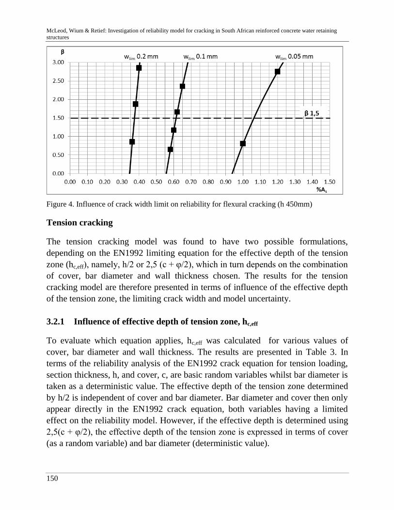
McLeod, Wium & Retief: Investigation of reliability model for cracking in South African reinforced concrete water retaining
structures
150
Figure 4. Influence of crack width limit on reliability for flexural cracking (h 450mm)
Tension cracking
The tension cracking model was found to have two possible formulations,
depending on the EN1992 limiting equation for the effective depth of the tension
zone (hc,eff), namely, h/2 or 2,5 (c + φ/2), which in turn depends on the combination
of cover, bar diameter and wall thickness chosen. The results for the tension
cracking model are therefore presented in terms of influence of the effective depth
of the tension zone, the limiting crack width and model uncertainty.
3.2.1 Influence of effective depth of tension zone, hc,eff
To evaluate which equation applies, hc,eff was calculated for various values of
cover, bar diameter and wall thickness. The results are presented in Table 3. In
terms of the reliability analysis of the EN1992 crack equation for tension loading,
section thickness, h, and cover, c, are basic random variables whilst bar diameter is
taken as a deterministic value. The effective depth of the tension zone determined
by h/2 is independent of cover and bar diameter. Bar diameter and cover then only
appear directly in the EN1992 crack equation, both variables having a limited
effect on the reliability model. However, if the effective depth is determined using
2,5(c + φ/2), the effective depth of the tension zone is expressed in terms of cover
(as a random variable) and bar diameter (deterministic value).
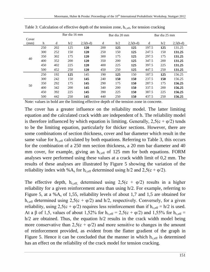
Moormann, Huber & Proske: Proceedings of the 10th International Probabilistic Workshop, Stuttgart 2012
151
Table 3: Calculation of effective depth of the tension zone, hc,eff, for tension cracking
Bar dia 16 mm Bar dia 20 mm Bar dia 25 mm
Cover
(mm) h d h/2 2,5(h-d) d h/2 2,5(h-d) d h/2 2,5(h-d)
40
250 202 125 120 200 125 125 197.5 125 131.25
300 252 150 120 250 150 125 247.5 150 131.25
350 302 175 120 300 175 125 297.5 175 131.25
400 352 200 120 350 200 125 347.5 200 131.25
450 402 225 120 400 225 125 397.5 225 131.25
500 452 250 120 450 250 125 447.5 250 131.25
50
250 192 125 145 190 125 150 187.5 125 156.25
300 242 150 145 240 150 150 237.5 150 156.25
350 292 175 145 290 175 150 287.5 175 156.25
400 342 200 145 340 200 150 337.5 200 156.25
450 392 225 145 390 225 150 387.5 225 156.25
500 442 250 145 440 250 150 437.5 250 156.25
Note: values in bold are the limiting effective depth of the tension zone in concrete.
The cover has a greater influence on the reliability model. The latter limiting
equation and the calculated crack width are independent of h. The reliability model
is therefore influenced by which equation is limiting. Generally, 2,5(c + φ/2) tends
to be the limiting equation, particularly for thicker sections. However, there are
some combinations of section thickness, cover and bar diameter which result in the
same value for hc,eff calculated by both equations. Referring to Table 3, this occurs
for the combination of a 250 mm section thickness, a 20 mm bar diameter and 40
mm cover, for example, giving an hc,eff of 125 mm for both equations. FORM
analyses were performed using these values at a crack width limit of 0,2 mm. The
results of these analyses are illustrated by Figure 5 showing the variation of the
reliability index with %As for hc,eff determined using h/2 and 2,5(c + φ/2).
The effective depth, hc,eff, determined using 2,5(c + φ/2) results in a higher
reliability for a given reinforcement area than using h/2. For example, referring to
Figure 5, at a %As of 1,55, reliability levels of about 1,7 and 1,5 are obtained for
hc,eff determined using 2,5(c + φ/2) and h/2, respectively. Conversely, for a given
reliability, using 2,5(c + φ/2) requires less reinforcement than if hc,eff = h/2 is used.
At a β of 1,5, values of about 1,52% for hc,eff = 2,5(c + φ/2) and 1,55% for hc,eff =
h/2 are obtained. Thus, the equation h/2 results in the crack width model being
more conservative than 2,5(c + φ/2) and more sensitive to changes in the amount
of reinforcement provided, as evident from the flatter gradient of the graph in
Figure 5. Hence it can be concluded that the manner in which hc,eff is determined
has an effect on the reliability of the crack model for tension cracking.
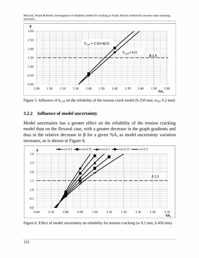
McLeod, Wium & Retief: Investigation of reliability model for cracking in South African reinforced concrete water retaining
structures
152
Figure 5. Influence of hc,eff on the reliability of the tension crack model (h 250 mm, wlim 0.2 mm)
3.2.2 Influence of model uncertainty
Model uncertainty has a greater effect on the reliability of the tension cracking
model than on the flexural case, with a greater decrease in the graph gradients and
thus in the relative decrease in β for a given %As as model uncertainty variation
increases, as is shown in Figure 6.
Figure 6. Effect of model uncertainty on reliability for tension cracking (w 0.2 mm, h 450 mm)
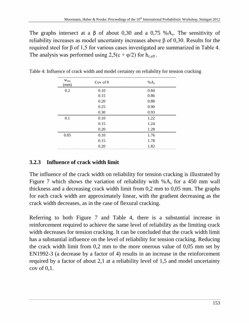
Moormann, Huber & Proske: Proceedings of the 10th International Probabilistic Workshop, Stuttgart 2012
153
The graphs intersect at a β of about 0,30 and a 0,75 %As. The sensitivity of
reliability increases as model uncertainty increases above β of 0,30. Results for the
required steel for β of 1,5 for various cases investigated are summarized in Table 4.
The analysis was performed using 2,5(c + φ/2) for hc,eff .
Table 4: Influence of crack width and model certainty on reliability for tension cracking
wlim
(mm) Cov of θ %As
0.2 0.10 0.84
0.15 0.86
0.20 0.88
0.25 0.90
0.30 0.93
0.1 0.10 1.22
0.15 1.24
0.20 1.28
0.05 0.10 1.76
0.15 1.78
0.20 1.82
3.2.3 Influence of crack width limit
The influence of the crack width on reliability for tension cracking is illustrated by
Figure 7 which shows the variation of reliability with %As for a 450 mm wall
thickness and a decreasing crack width limit from 0,2 mm to 0,05 mm. The graphs
for each crack width are approximately linear, with the gradient decreasing as the
crack width decreases, as in the case of flexural cracking.
Referring to both Figure 7 and Table 4, there is a substantial increase in
reinforcement required to achieve the same level of reliability as the limiting crack
width decreases for tension cracking. It can be concluded that the crack width limit
has a substantial influence on the level of reliability for tension cracking. Reducing
the crack width limit from 0,2 mm to the more onerous value of 0,05 mm set by
EN1992-3 (a decrease by a factor of 4) results in an increase in the reinforcement
required by a factor of about 2,1 at a reliability level of 1,5 and model uncertainty
cov of 0,1.
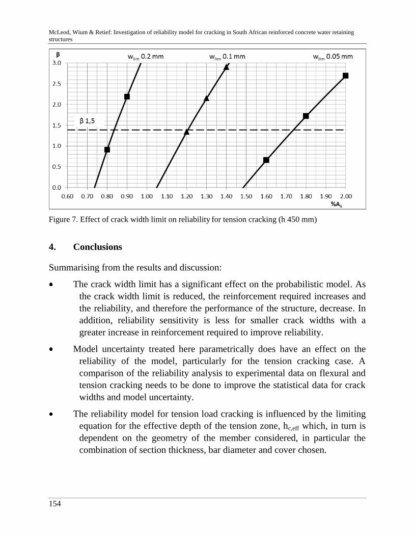
McLeod, Wium & Retief: Investigation of reliability model for cracking in South African reinforced concrete water retaining
structures
154
Figure 7. Effect of crack width limit on reliability for tension cracking (h 450 mm)
4. Conclusions
Summarising from the results and discussion:
The crack width limit has a significant effect on the probabilistic model. As
the crack width limit is reduced, the reinforcement required increases and
the reliability, and therefore the performance of the structure, decrease. In
addition, reliability sensitivity is less for smaller crack widths with a
greater increase in reinforcement required to improve reliability.
Model uncertainty treated here parametrically does have an effect on the
reliability of the model, particularly for the tension cracking case. A
comparison of the reliability analysis to experimental data on flexural and
tension cracking needs to be done to improve the statistical data for crack
widths and model uncertainty.
The reliability model for tension load cracking is influenced by the limiting
equation for the effective depth of the tension zone, hc,eff which, in turn is
dependent on the geometry of the member considered, in particular the
combination of section thickness, bar diameter and cover chosen.

Moormann, Huber & Proske: Proceedings of the 10th International Probabilistic Workshop, Stuttgart 2012
155
References
[1] Beeby AW, Narayanan RS (2005). Designer’s guide to EN1992-1-1 and
EN1992-1-2: Design of concrete structures. General rules and rules for
buildings and structural fire design. Thomas Telford.
[2] BS 8007: Design of concrete structures for retaining aqueous liquids. BSI
1987
[3] BS EN 1990: Eurocode 0: Basis of structural design. BSI 2002.
[4] BS EN 1992-1: Eurocode 2: Design of concrete structures – Part 1:
General requirements. BSI 2004.
[5] BS EN 1992-3: Eurocode 2: Design of Concrete Structures – Part 3:
Liquid Retaining and Containment Structures. BSI 2006.
[6] Holicky M (2009). Reliability analysis for structural design. SUN Media
Stellenbosch.
[7] Joint Committee on Structural Safety. Interpretation of Uncertainties and
Probabilities in Civil Engineering Decision Analysis. Background
documents on risk assessment in engineering. Document No. 2. JCSS,
Zurich 2008. http://www.jcss.ethz.ch/.
[8] Quan Q, Gengwei Z (2002). Calibration of reliability index of RC beams
for serviceability limit state of maximum crack width. Journal of Reliability
Engineering and System Safety. No. 75 (2002), pg 359 – 366.
[9] SANS 10100-1: The structural use of concrete: Part 1: Design. South
African Bureau of Standards. Pretoria 2000.
[10] SANS 10100-3(Draft): Design of concrete water retaining structures.
WRC Project group with the Institute of Structural Engineering. 2010
[11] SANS 10160: Basis of structural design and actions for buildings and
industrial structures. South African Bureau of Standards. Pretoria 2011.
[12] Wium, JA (2008). Report April 2008: Basis of design and materials. The
development and calibration of South Africa’s National Standards for
water retaining structures. WRC Project No. K5/1764, Water Research
Commission of South Africa, Pretoria, SA

McLeod, Wium & Retief: Investigation of reliability model for cracking in South African reinforced concrete water retaining
structures
156
Moormann, Huber & Proske: Proceedings of the 10th International Probabilistic Workshop, Stuttgart 2012
* The opinions expressed in this paper are the author’s and do not necessarily reflect the policy or position of
ABN AMRO. 157
Challenges in modelling in banking:
behaviour
Remko Riebeek
Integrated Risk Management
ABN AMRO Bank N.V.*
Abstract: In this paper we argue that behavioural phenomena are at the heart
of improvements that risk modelling requires to overcome the weaknesses that
have been laid bare in the credit crisis. These behavioural aspects need to be
addressed both in the models themselves and in the processes around the use of
the models.
1 Introduction
The credit crisis in 2007/2008 is closely connected to risk models and, in par-
ticular, the use of these models in the financial sector. On the one hand are
risk models seen as one of the causal factors for the crisis, on the other hand is
the impact of the credit crisis profound on the modelling landscape. In this
paper, we will touch upon the most important issues that have become appar-
ent from the credit crisis that are related to the models. We will argue that an
important concept that is required to solve these issues is the understanding of
behavioural aspects related to how people act under uncertainty.
This is important because one of the consequences of the credit crisis is that
decision makers in financial institutions (but, in particular, also in the political
surroundings thereof) have lost confidence in the statistical toolkit, thereby
relying stronger on their intuitions and gut feelings. One can only question
whether or even when this approach will lead to new disasters. In stark con-
trast with the above we find that regulators and supervisors are continuously
and quickly increasing the pressure on financial institutions to lift their stand-
ards of risk modelling. These contrasting views are already an enormous chal-
lenge for risk modellers and risk managers, but it is even enlarged by another:
the current macro-economic climate, with its extremely volatile financial
markets and uncertainty (e.g. in the Eurozone). This situation is located on the

Riebeek: Challenges in modelling in banking: bahaviour
158
extreme end of existing risk models, where data is scarce and confidence in-
tervals are difficult to determine.
The science of behavioural economics is not new, but has gained popularity
over the last years. The ground breaking research in this area was done by the
duo of Amos Tversky and Daniel Kahneman, the latter of them, as a psy-
chologist, receiving the Nobel prize for economics for their research in this
area in 2002. It must be mentioned that already Keynes was very aware that
economics was a behavioural science. It may even be said that a lot of the
problems that led to the credit crisis were the result of the trend in economics
to consider the economy as an ergodic system, thereby being able to use
“physics resembling” mathematical models to describe the economic reality.
Recently, Kahneman published an excellent book that brings forward the
whole field of behavioural aspects of judgement and action under uncertainty
in an uncomplicated fashion without sacrificing the required nuancing depth.
The application of behavioural aspects in finance were pioneered by Hersh
Shefrin, see e.g. [8].
In the following chapters we will treat three important topics for risk model-
lers to address in the world after the credit crisis.
First, we will look at why, when using the models developed to estimate the
risks of financial instruments, the risks in the financial world could build up
with the collapse of Lehman Brothers and its aftermath as a result. We will
see that excessive optimism, overconfidence and, possibly, loss aversion were
key ingredients and that understanding these phenomena is necessary to write
a “manual” for any financial risk model.
Second, we will look at the risk types that are the current focus of modelling
in financial institutions and conclude that more emphasis should be put in
modelling operational risk and strategic risk. Currently, both these risk types
are measured with a strong use of expert opinion. It is clear that debiasing
these expert opinion (especially when performed in groups) is key. Further-
more, both risk types are caused by actions and interactions and beliefs of
people: another clear reference for applying behavioural aspects.
Third, we will take a look at risk management in extreme (crisis) situations. In
almost all cases we see that group dynamics take over from rationality. Un-
derstanding how this works will be necessary to understand and predict the
current economic situation and to act wisely.
Moormann, Huber & Proske: Proceedings of the 10th International Probabilistic Workshop, Stuttgart 2012
* The opinions expressed in this paper are the author’s and do not necessarily reflect the policy or position of
ABN AMRO. 159
2 Failed Models or Failed Model Use
If the credit crisis has taught us one thing, it is that models are used by hu-
mans and made by humans. Finding the boundaries and holes of models,
tweaking models, “gaming the system”, ignoring model constraints, misusing
models outside of the context are all part of real corporate life, as well as giv-
ing in to pressures to implementing unsound statistics and cleaning calibrating
data from undesirable elements.
Stories exist all over the place of managers demanding models to provide
more optimistic results and risk managers and their modelling teams giving in
to these demands or, if not, being fired. It is clear that many AAA-rated fi-
nancial products were not that risk-free and that capital models were underes-
timating the capital required to protect the company against insolvency with a
99.95% or 99.98% confidence level. Note that this 99.9x% already in itself is
a difficult notion to get a mental grasp on and that it is often explained as a 1
in 2000 years event. In terms of ordinary people this translates to extremely
unlikely or, better said, too unrealistic to feel the need to prepare for. Remem-
bering that 2000 years ago we were in the times of the Roman Empire and so
many unpredictable revolutions happened afterwards, this should also not
come as a surprise.
Banks, insurance companies, investors, regulators and supervisory bodies all
relied heavily on these (economic) capital models and the Basel II regulation
made it possible to use internal models in an attempt to make regulatory con-
straints more risk sensitive. The fact that less required capital equals more
profit (in the short term) is a strong incentive to construct models that reduce
capital needs to a minimum. The before mentioned “1 in 2000 years” explana-
tion does not help to feel the need to suppress this incentive and the many pa-
rameters an internal and complex model has, can be used by the modeller to
give companies the ability to play with capital models.
It seems that regulators have overlooked or underestimated the adverse effects
of the allowance of internal risk models to compute required capital, in par-
ticular of how it influences the behaviour of managers. It also seems that
managers themselves have underestimated the risks of their companies’ strat-
egies. The literature suggests that this behaviour often comes from an illusion
of control: overestimation of one’s own degree of control over potential ad-
verse situations.
To protect the value of their profession, the key challenge for modellers in
risk management is to unmistakably and comprehensibly define and describe

Riebeek: Challenges in modelling in banking: bahaviour
160
the intended use of the designed models, thereby including knowledge on po-
tential misuse.
The current Basel III proposals (e.g. the introduction of leverage ratio and the
return to core equity capital) show that regulators seek to use simpler, central-
ly designed models to determine the size of regulatory capital in banks. This
will relieve risk modellers in those companies somewhat as their modelling
efforts will less impact the amount of required regulatory capital.
3 Models that matter
Banks have traditionally focused their risk modelling efforts on their core
processes: credit risk and, later, market risk. Regulation has followed these
developments (in particular with the so called Basel agreements), the focus
until recently being on credit risk and market risk. Only with the revision to
Basel II ([1]) from 2006, operational risk has become another important topic
of interest, with limited attention also for other risk types. It must be said that
in practice modelling operational risk remains a difficult task. With the devel-
opment of Basel III also other risk types, such as liquidity risk, have gotten to
the forefront. It is interesting to see whether these are indeed the most im-
portant risk types for a bank’s solvability.
James Lam and others [6] have done research on why companies underper-
form. Their results are summarised in the table below:
Table 1. Strategic risk identified as the major cause for financial distress (copied from [6])
Organization Research Methodology Key Findings
James Lam & Associ-
ates (2004)
The Corporate Execu-
tive Board (2005)
Deloitte Research
(2005)
S&P 500 (1982-2003)
One month stock price decline of 30%
or greater relative to the S&P 500
Fortune 1000 companies (1998-2002)
Top 20% of companies with the great-
est market value declines
Thomson Financial Global 1000
Companies (1994-2003)
One-month stock price decline rela-
tive to the Morgan Stanley Financial
61% were exposed to strategic
risks
30% were exposed to opera-
tional risks
9% were exposed to financial
risks
65% were exposed to strategic
risks
20% were exposed to opera-
tional risks
15% were exposed to finan-
cial risks
Among the 100 largest declines:
66 involved strategic risks
62 involved external events
61 involved operational risks
Moormann, Huber & Proske: Proceedings of the 10th International Probabilistic Workshop, Stuttgart 2012
* The opinions expressed in this paper are the author’s and do not necessarily reflect the policy or position of
ABN AMRO. 161
World Index 37 involved financial risks
The conclusion that can be drawn from this research is that strategic risk and
operational risk are the risk types that should require the most attention and
that these are undervalued in the regulatory framework.
One of the reasons for not including these risk types in the regulatory frame-
work is the apparent difficulty in modelling them. The difficulty lies for the
larger part in the behavioural aspects of both of these risk types. These aspects
can be seen in two parts of the modelling process.
First, the decisions taken that lead to operational or strategic disasters often
possess a behavioural character. As an example of strategic risks, we can
think of the decision process to enter a new market or the decision to develop
a new corporate image that can be marred by excessive optimism and overcon-
fidence. As examples of operational risks, we can think of the Barings/Nick
Leeson disaster in 1995 and the enormous trading loss in the Jérôme
Kerviel/Société Générale case in 2008 (see [9]) or, more recently, the JP
Morgan case that were allegedly caused by a combination of sure loss aver-
sion and interactions between traders, back office and control functions.
Second, the current practice of estimating the risks is the intensive use of ex-
pert opinions, often in group settings. In these workshop sessions, experts are
asked to estimate likelihood and impact of a number of identified risks. Both
the biases and heuristics of the experts as well as the group settings are a bowl
full of behavioural problems that make the outcome of the estimates question-
able if there is no structural attention for the influence of these aspects on the
outcomes. As examples we mention availability bias: the phenomenon that
people overvalue information that is readily available (e.g. an incident that
just occurred) and groupthink: the phenomenon that consensus leads to not
exploring other paths of potential developments.
In my opinion, these phenomena will have to play an important role in the
development of models for these risk types, given the influence these have on
the outcomes.
4 Models in extreme situations
After the Lehman Brothers collapse on September, 15th 2008, the financial
markets are in a state of continuous high tension. The uncertainty of the cre-
ditworthiness of sovereigns, financial institutions and companies is perceived
high and (therefore?) any newsflash and rumour has a high impact on market

Riebeek: Challenges in modelling in banking: bahaviour
162
sentiment. This market sentiment is a typical subject of study of behavioural
risk management.
A common behavioural phenomenon in stress situations is for example sure
loss aversion: people and financial institutions hold on to assets that have de-
creased considerably in value betting on the small chance that their value will
increase again into profitable terrain, thereby seeing the asset values drop fur-
ther.
A key element in (not) predicting this extreme situation has been the limited
historic horizon (there are almost no known implementations that use data
that goes all the way back to the great crash in 1929) that is being used in
simulation and stress testing exercises that are often based on replaying his-
torical stress events, thereby limiting the influence of other types of potential
events. We now see a move by regulation (e.g. EBA [4] and FED [2]) to rely
more and more on stress testing. This development can be an important im-
provement of risk models as it may estimate extreme events more reliably. Of
course, questions still exist around the methodology of stress testing. Some
are mentioned in [7]. Again, a high level of human judgement is involved in
designing and performing stress testing scenarios, which leads us back to the
main theme of this paper.
As a final remark, the Eurozone sovereign and financial sector problems of
the last years have shown that politicians play an important role in the direc-
tion crises take. The impact of the dynamics of political discourse on the fi-
nancial markets is high. This political uncertainty is most often included in
risk management by analysing several outcomes of scenarios into stress test-
ing exercises. Nevertheless, even though a company should be prepared for
various outcomes of scenarios assigning probabilities to these scenarios, it is
in practice a topic of heavy discussion. Therefore, the study of interactions of
actors in negotiations (i.e. game theory) could be another topic of interest for
risk modellers. It is suggested by [3] that probabilities of this type can be pre-
dicted with a reasonable level of confidence.
4.1 Literature
[1] Bank of International Settlements: Basel II: Revised International Capital Frame-
work, http://www.bis.org/publ/bcbsca.htm , 2006
[2] Board of Governors of the Federal Reserve: Comprehensive Capital Analysis and
Review 2012: Methodology and Results for Stress Scenario Projections,
http://www.federalreserve.gov/newsevents/press/bcreg/bcreg20120313a1.pdf, March
13, 2012
[3] Bruce Bueno de Mesquita: The Predictioneer’s Game, 2009

Moormann, Huber & Proske: Proceedings of the 10th International Probabilistic Workshop, Stuttgart 2012
* The opinions expressed in this paper are the author’s and do not necessarily reflect the policy or position of
ABN AMRO. 163
[4] European Banking Authority: EU-wide stress testing, http://www.eba.europa.eu/EU-
wide-stress-testing.aspx
[5] Kahneman, Daniel: Thinking, fast and slow, 2011
[6] Lam, James: ERM and Corporate Strategy – Driving Business Performance through
Risk Intelligence, webinar (July 17, 2012)
[7] John Lester, Peter Reynolds, Til Schuermann, Dylan Walsh: Strategic Capital; De-
fining an effective real-world view of capital,
http://www.oliverwyman.com/strategic-capital-defining-an-effective-real-world-
view-of-capital.htm, 2012
[8] Shefrin, Hersh: Behavioral Corporate Finance – Decisions that Create Value, 2007
[9] Shefrin, Hersh: Ending the Management Illusion, 2008

Riebeek: Challenges in modelling in banking: bahaviour
164

Moormann, Huber & Proske: Proceedings of the 10th International Probabilistic Workshop, Stuttgart 2012
165
Resistance Factor Calibration
of Drilled Shafts for Bridge Foundations
D. Bach, P.H.A.J.M. van Gelder, K.J. Bakker, and J.K. Vrijling
Delft University of Technology, Delft, The Netherlands
Abstract: Calibrating resistance factors for drilled shafts is to insure safety
degrees for foundation structures with high load effects from a superstructure
system with target reliability levels. As this is accomplished under conditions
of uncertainty, probabilistic analyses are necessary in the development of such
probability-based design methods. A method for load and resistance factor
design (LRFD) will be presented, and reliability-based methods for calibrating
the resistance factors are described in this paper. Methods which consist of
first-order second moment (FOSM), first-order reliability method (FORM), and
Monte Carlo simulation (MCS) are used to calibrate these factors for 16 cases
of calculation, which are based on a drilled shaft database covering various
types of soil, resistance prediction methods, and construction methods. The
resistance factors are determined for a set of assigned load factors to meet
specified target reliability indices. Moreover, correlation analyses between the
determined resistance factors which are calibrated according to reliability
methods are also considered herein. Through obtained results, some extra
findings are illustrated in this paper.
1 Introduction
The allowable stress design (ASD), also called the working stress design
(WSD) method, has been used in civil engineering since the early 1800s.
Under ASD, the design load, which consists of the actual forces applied to the
piles, has to be less than the resistance divided by a single factor of safety.
This method has several shortcomings, the most significant of which is that it
does not provide a consistent framework for incorporating the individual
sources of risk into the design. In fact, each component of the load and the
resistance has a different level of variability and uncertainty.
Bach, van Gelder, Bakker & Vrijling: Resistance Factor Calibration of Drilled Shafts for Bridge Foundations
166
In the 1950s, the demand for the more economical design of piles brought
about the use of the limit state design (LSD) method. Two types of limit states
are usually considered, ultimate limit state (ULS), and serviceability limit
state (SLS). ULS pertains to structural safety and involves structural collapse
or, in relation to piles, the ultimate bearing capacity of soils. SLS pertains to
conditions, such as excessive deformations and settlements or deterioration of
the structure that would affect the performance of the structure under
expected working loads. The format of limit state design equations involves
the application of partial factors to increase the loads and to decrease the
resistances. This approach represents a fundamental improvement over the
single factor of safety in ASD because the partial factors are applied directly
to the uncertain quantities of loads and resistances.
The partial factors were determined subjectively based on two criteria: (i) a
larger partial factor should be applied to a more uncertain quantity; (ii) the
partial factors should result in approximately the same dimensions as those
from traditional practice. This approach did not satisfy one of the basic
requirements of LSD because it is impossible to demonstrate the occurrence
of each limit state (Brown et al. [6]). The next logical step in LSD has been to
apply probabilistic reliability analysis to establish the partial factors, in order
to account for the uncertainty and variability for loads and resistances. One of
the advantages of this approach is that all components of the structure,
including the foundations, can be designed to a uniform level of safety. The
LSD method based on the probabilistic reliability analysis has been used
increasingly with a new name as the load and resistance factor design (LRFD)
method, in which the partial factors applied to loads are termed load factors
and those applied to resistances are resistance factors. Each resistance factor
is the product of a calibration study in which a limit state function (LSF) is
evaluated to predict a specific component of resistance (e.g., side or base or
both types of resistance) to a specified target reliability level.
As described by Withiam et al. [13], calibrating load factors and resistance
factors can be carried out by the use of: (i) judgment; (ii) fitting to other codes
or past practice; (iii) reliability-based analysis; or (iv) a combination of
approaches. Only the third approach, reliability-based analysis, satisfies the
objective of LSD, and establishes load and resistance factors to achieve a
defined target reliability level. Several comprehensive works based on the
reliability analysis were conducted for the resistance factor calibration, for
example, FOSM was used by Barker et al. [5], FORM was used by
Paikowsky et al. [12] and MCS was utilized in the works of Allen et al. [2]
and Abu-Farsakh and Yu [1].
Moormann, Huber & Proske: Proceedings of the 10th International Probabilistic Workshop, Stuttgart 2012
167
In this paper, resistance factors are calibrated according to different
reliability-based methods. A database, which involves sixteen cases of
calculation of axially loaded drilled shafts, is collected and computed under
the ultimate limit state for strength I. Each case is represented by a soil type, a
resistance prediction method and a construction method. The resistance
factors are calibrated with specified target reliability levels and different span
lengths of bridges. From the obtained results, the relationships between
resistance factors and statistical parameters of the resistance are formulated.
Furthermore, the correlations between resistance factors calibrated by
reliability methods are presented and discussed as well.
2 Reliability-Based Design Methods
According to Ayyub et al. [4], there are two primary approaches for the
reliability-based design: (i) load and resistance factor design (LRFD); and (ii)
direct reliability-based design. The LRFD approach is called the level I
reliability method. Level I reliability methods use partial safety factors
(PSF's) that are reliability based; but the methods do not require explicit use
of the probabilistic description of the random variables. The direct reliability-
based design approach can include level II and/or level III reliability methods.
Level II reliability methods (e.g. FOSM, FORM) are based on the moments
(mean and variance) of random variables, and sometimes, with a linear
approximation of non-linear limit state functions. Level III reliability methods
such as numerical integration according to the Riemann procedure, MCS, use
the complete probabilistic characteristics of the random variables.
2.1 Reliability-based design philosophy
The reliability-based design procedure requires defining limit state functions
that correspond to limit states for significant failure modes. A general form
for the limit state function for a structural component is given by:
(1)
Where g is the limit state function, R is the resistance (or strength), and Q is
the load effect on the structural component. The failure is defined in the
region where g is less than zero or R is less than Q, that is g < 0 or R < Q.
Whereas, the safety is defined in the region where g is greater than zero or R
is greater than Q, that is g > 0 or R > Q.
The reliability-based design approach assumes the resistance R and the load Q
to be random variables. The frequency distributions, permanently called the
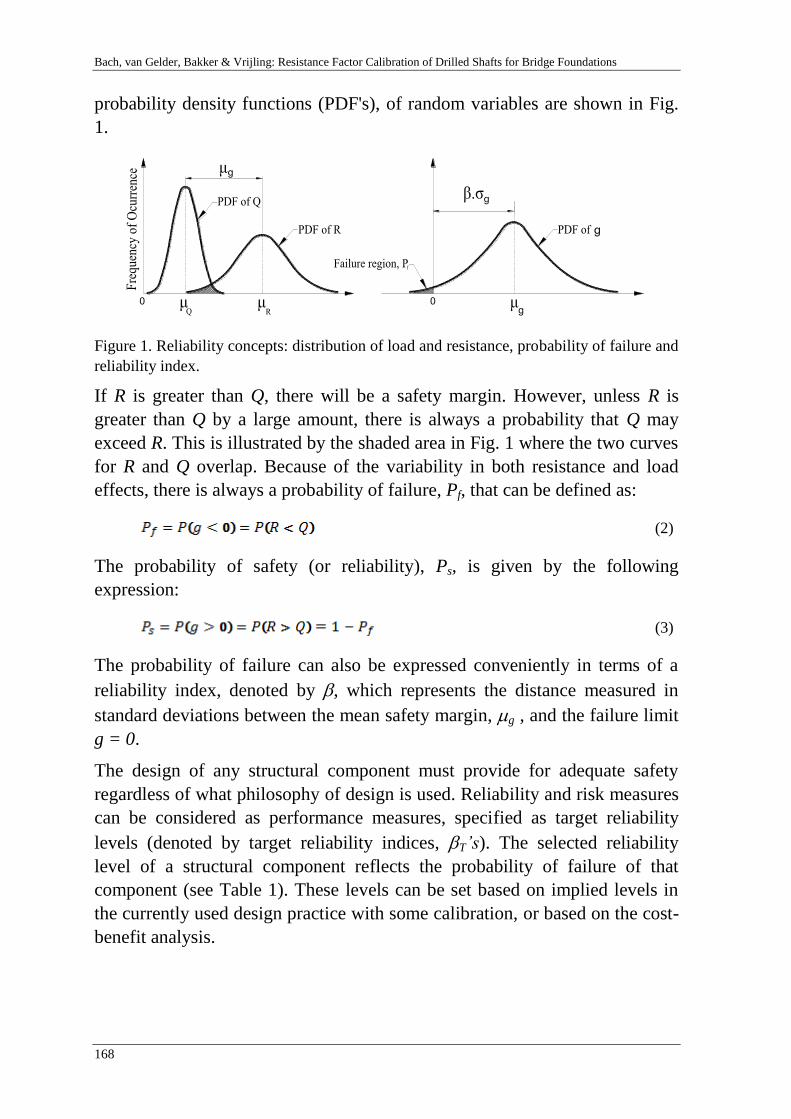
Bach, van Gelder, Bakker & Vrijling: Resistance Factor Calibration of Drilled Shafts for Bridge Foundations
168
probability density functions (PDF's), of random variables are shown in Fig.
1.
Figure 1. Reliability concepts: distribution of load and resistance, probability of failure and
reliability index.
If R is greater than Q, there will be a safety margin. However, unless R is
greater than Q by a large amount, there is always a probability that Q may
exceed R. This is illustrated by the shaded area in Fig. 1 where the two curves
for R and Q overlap. Because of the variability in both resistance and load
effects, there is always a probability of failure, Pf, that can be defined as:
(2)
The probability of safety (or reliability), Ps, is given by the following
expression:
(3)
The probability of failure can also be expressed conveniently in terms of a
reliability index, denoted by , which represents the distance measured in
standard deviations between the mean safety margin, g , and the failure limit
g = 0.
The design of any structural component must provide for adequate safety
regardless of what philosophy of design is used. Reliability and risk measures
can be considered as performance measures, specified as target reliability
levels (denoted by target reliability indices, T’s). The selected reliability
level of a structural component reflects the probability of failure of that
component (see Table 1). These levels can be set based on implied levels in
the currently used design practice with some calibration, or based on the cost-
benefit analysis.
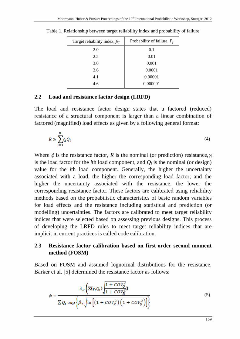
Moormann, Huber & Proske: Proceedings of the 10th International Probabilistic Workshop, Stuttgart 2012
169
Table 1. Relationship between target reliability index and probability of failure
Target reliability index, T Probability of failure, Pf
2.0
2.5
3.0
3.6
4.1
4.6
0.1
0.01
0.001
0.0001
0.00001
0.000001
2.2 Load and resistance factor design (LRFD)
The load and resistance factor design states that a factored (reduced)
resistance of a structural component is larger than a linear combination of
factored (magnified) load effects as given by a following general format:
(4)
Where is the resistance factor, R is the nominal (or prediction) resistance,i
is the load factor for the ith load component, and Qi is the nominal (or design)
value for the ith load component. Generally, the higher the uncertainty
associated with a load, the higher the corresponding load factor; and the
higher the uncertainty associated with the resistance, the lower the
corresponding resistance factor. These factors are calibrated using reliability
methods based on the probabilistic characteristics of basic random variables
for load effects and the resistance including statistical and prediction (or
modelling) uncertainties. The factors are calibrated to meet target reliability
indices that were selected based on assessing previous designs. This process
of developing the LRFD rules to meet target reliability indices that are
implicit in current practices is called code calibration.
2.3 Resistance factor calibration based on first-order second moment
method (FOSM)
Based on FOSM and assumed lognormal distributions for the resistance,
Barker et al. [5] determined the resistance factor as follows:
(5)
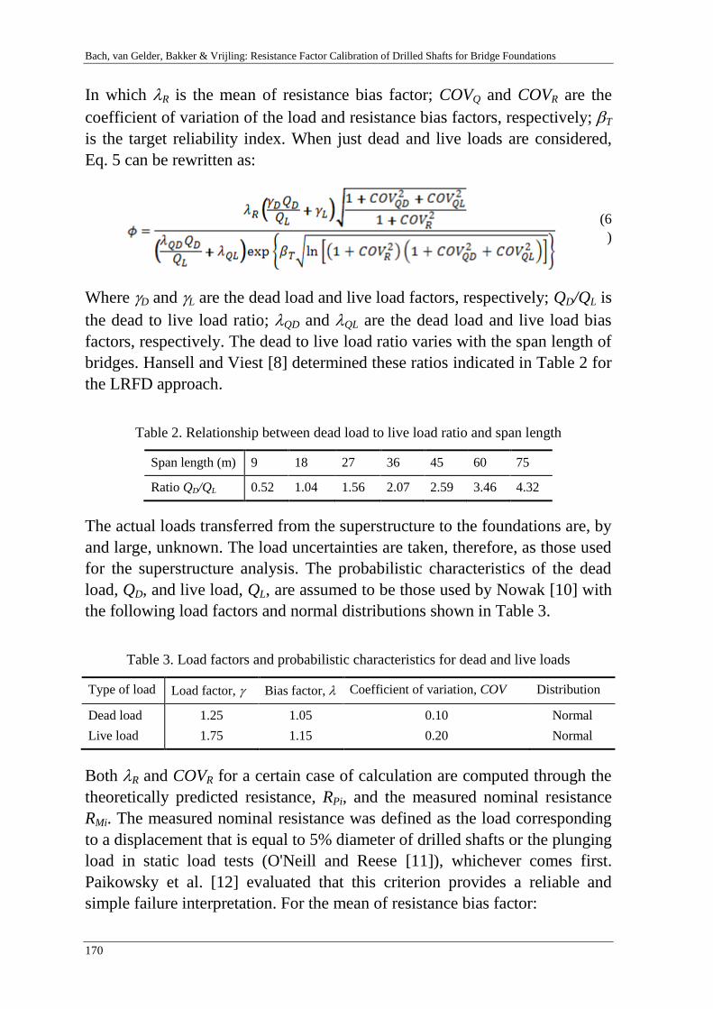
Bach, van Gelder, Bakker & Vrijling: Resistance Factor Calibration of Drilled Shafts for Bridge Foundations
170
In which R is the mean of resistance bias factor; COVQ and COVR are the
coefficient of variation of the load and resistance bias factors, respectively; T
is the target reliability index. When just dead and live loads are considered,
Eq. 5 can be rewritten as:
(6
)
Where D and L are the dead load and live load factors, respectively; QD/QL is
the dead to live load ratio; QD and QL are the dead load and live load bias
factors, respectively. The dead to live load ratio varies with the span length of
bridges. Hansell and Viest [8] determined these ratios indicated in Table 2 for
the LRFD approach.
Table 2. Relationship between dead load to live load ratio and span length
Span length (m) 9 18 27 36 45 60 75
Ratio QD/QL 0.52 1.04 1.56 2.07 2.59 3.46 4.32
The actual loads transferred from the superstructure to the foundations are, by
and large, unknown. The load uncertainties are taken, therefore, as those used
for the superstructure analysis. The probabilistic characteristics of the dead
load, QD, and live load, QL, are assumed to be those used by Nowak [10] with
the following load factors and normal distributions shown in Table 3.
Table 3. Load factors and probabilistic characteristics for dead and live loads
Type of load Load factor, Bias factor, Coefficient of variation, COV Distribution
Dead load
Live load
1.25
1.75
1.05
1.15
0.10
0.20
Normal
Normal
Both R and COVR for a certain case of calculation are computed through the
theoretically predicted resistance, RPi, and the measured nominal resistance
RMi. The measured nominal resistance was defined as the load corresponding
to a displacement that is equal to 5% diameter of drilled shafts or the plunging
load in static load tests (O'Neill and Reese [11]), whichever comes first.
Paikowsky et al. [12] evaluated that this criterion provides a reliable and
simple failure interpretation. For the mean of resistance bias factor:
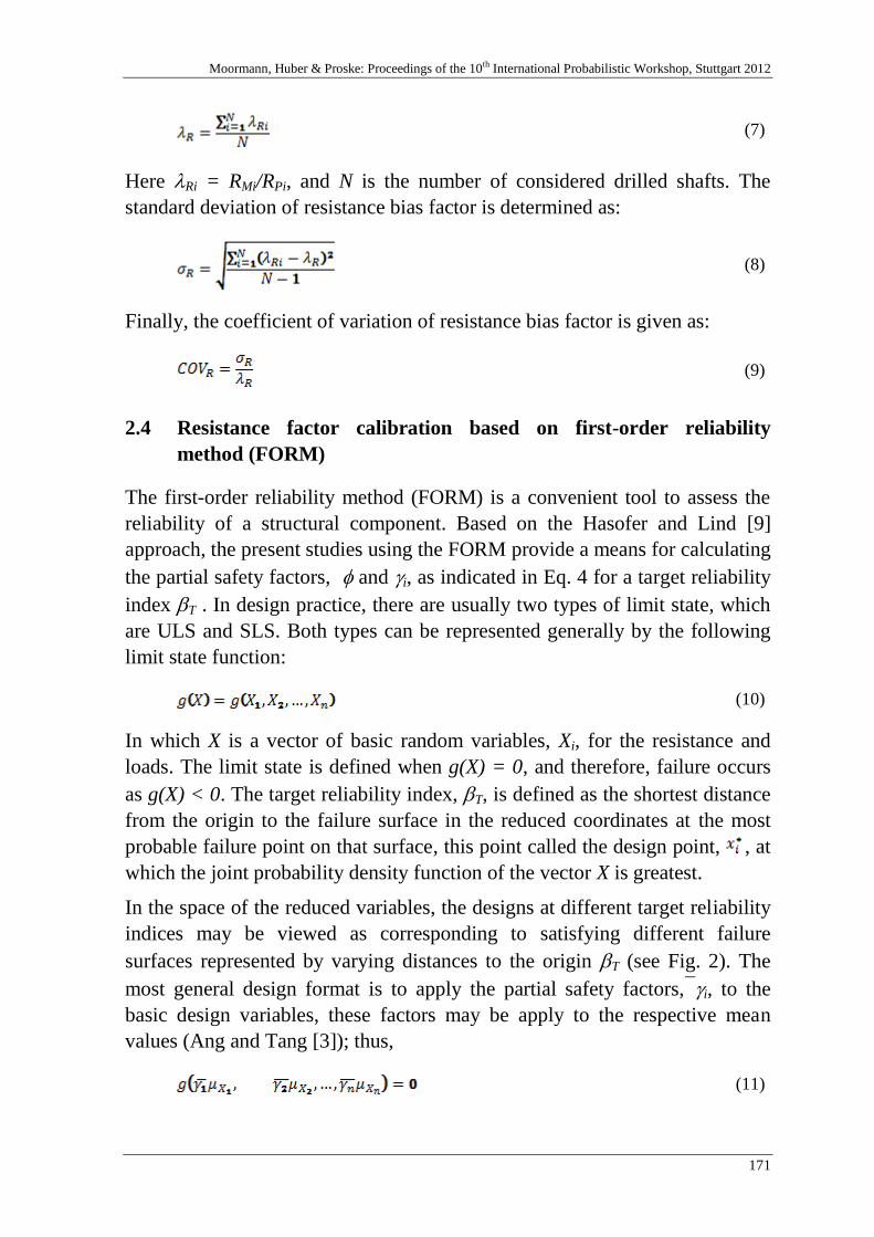
Moormann, Huber & Proske: Proceedings of the 10th International Probabilistic Workshop, Stuttgart 2012
171
(7)
Here Ri = RMi/RPi, and N is the number of considered drilled shafts. The
standard deviation of resistance bias factor is determined as:
(8)
Finally, the coefficient of variation of resistance bias factor is given as:
(9)
2.4 Resistance factor calibration based on first-order reliability
method (FORM)
The first-order reliability method (FORM) is a convenient tool to assess the
reliability of a structural component. Based on the Hasofer and Lind [9]
approach, the present studies using the FORM provide a means for calculating
the partial safety factors, and i, as indicated in Eq. 4 for a target reliability
index T . In design practice, there are usually two types of limit state, which
are ULS and SLS. Both types can be represented generally by the following
limit state function:
(10)
In which X is a vector of basic random variables, Xi, for the resistance and
loads. The limit state is defined when g(X) = 0, and therefore, failure occurs
as g(X) < 0. The target reliability index, T, is defined as the shortest distance
from the origin to the failure surface in the reduced coordinates at the most
probable failure point on that surface, this point called the design point, , at
which the joint probability density function of the vector X is greatest.
In the space of the reduced variables, the designs at different target reliability
indices may be viewed as corresponding to satisfying different failure
surfaces represented by varying distances to the origin T (see Fig. 2). The
most general design format is to apply the partial safety factors,i, to the
basic design variables, these factors may be apply to the respective mean
values (Ang and Tang [3]); thus,
(11)
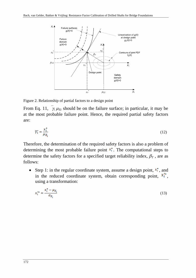
Bach, van Gelder, Bakker & Vrijling: Resistance Factor Calibration of Drilled Shafts for Bridge Foundations
172
Figure 2. Relationship of partial factors to a design point
From Eq. 11, i Xi should be on the failure surface; in particular, it may be
at the most probable failure point. Hence, the required partial safety factors
are:
(12)
Therefore, the determination of the required safety factors is also a problem of
determining the most probable failure point . The computational steps to
determine the safety factors for a specified target reliability index, T , are as
follows:
Step 1: in the regular coordinate system, assume a design point, , and
in the reduced coordinate system, obtain corresponding point, ,
using a transformation:
(13)
Moormann, Huber & Proske: Proceedings of the 10th International Probabilistic Workshop, Stuttgart 2012
173
Where Xi and Xi are the mean value and the standard deviation of
basic random variable Xi, respectively. The mean value of the vector of
basic random variables is often used as an initial value for the design
point.
Step 2: if the distribution of basic random variables is non-normal,
approximate this distribution with an equivalent normal distribution at
the design point, having the same tail area and ordinate of the
probability density function, that is an equivalent mean:
(14)
and an equivalent standard deviation:
(15)
Where and are the mean and standard deviation of the
equivalent normal distribution for variable Xi, respectively. FXi( ) and
fXi( ) are the original cumulative distribution function (CDF) and
original probability density function (PDF) of variable, Xi, evaluated at
the design point respectively. and are the CDF and PDF of the
standard normal distribution, respectively.
Step 3: set = - i , in which is the direction cosine determined
as follows:
(16)
Where:
(17)
Step 4: a new design point obtained as:
(18)
Bach, van Gelder, Bakker & Vrijling: Resistance Factor Calibration of Drilled Shafts for Bridge Foundations
174
In general, the determination of requires an iterative solution. Steps 1 to 3
are repeated until convergence of is achieved. Then, through Eq. 12, the
resistance factor, , and the load factors, i, are obtained as:
(19)
and:
(20)
Where r* and are the design points of resistance and loads, respectively. R
and Qi are the mean values of resistance and loads, respectively. The
resistance factor is generally less than one, whereas the load factors are
greater than one.
As specified by Paikowsky et al. [12], for a given target reliability index and
probability distributions for resistance and loads, the partial safety factors
determined by the FORM approach may differ with failure mode. For this
reason, the calibration of the partial safety factors is to maintain the same
values for all loads at different failure modes. In the case of geotechnical
codes, the resistance factor calibration is performed for a set of load factors
already specified in the structural code (see Section 2.3). Thus, the load
factors are fixed, the following algorithm is used to determine the resistance
factor only:
For a given target reliability index, probability distributions and
statistical parameters of load and resistance variables, compute mean
resistance using FORM.
With the mean value of resistance computed above, the resistance
factor, , can be revised for a given set of load factors as follows:
(21)
2.5 Resistance factor calibration based on Monte Carlo simulation
(MCS)
This paper follows the calibration procedure based on MCS as recommended
by Allen et al. [2] to determine the resistance factor of drilled shafts. The dead
and live loads are considered abiding the strength I ultimate limit state. Thus,
the limit state function can be written as:
(22)
Moormann, Huber & Proske: Proceedings of the 10th International Probabilistic Workshop, Stuttgart 2012
175
In which RM, QMD, and QML are the measured nominal resistance, the mean
value of dead load and live load, respectively. Implement bias factors, R,
QD, and QL for the resistance, dead load and live load, respectively, we have:
(23)
Combine Eq. 4 into Eq. 23, after several transformations, the limit state
function can be rewritten as:
(24)
Where all terms in Eq. 24 are the same as those aforementioned in Section
2.3.
MCS was used to generate random numbers that are needed to independently
extrapolate the cumulative distribution function (CDF) value for each random
variable in the calibration process. In this calibration, there are three random
variables which are resistance, dead load and live load bias factors. The
computation steps are as follows:
Step 1: assign a target reliability index, T .
Step 2: select a trial resistance factor, .
Step 3: generate random numbers for each set of bias factors R, QD
and QL.
Step 4: define the limit state function g as described in Eq. 24. Find the
number of cases in which g ≤ 0. The probability of failure is then
computed as:
(25)
Where NS is the number of simulations. In this paper, the number of
simulations was used as 5x10⁴. The corresponding calculated reliability
index, , is then defined as:
(26)
Where -1 is the inverse CDF of the standard normal distribution. If the
calculated reliability index, , is different from the specified target
reliability index, T , the trial resistance factor, , in Step 2 should be
changed and a new iteration needs to be repeated until |-T|≤
tolerance.
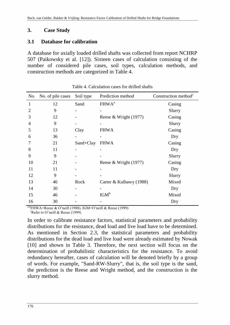
Bach, van Gelder, Bakker & Vrijling: Resistance Factor Calibration of Drilled Shafts for Bridge Foundations
176
3. Case Study
3.1 Database for calibration
A database for axially loaded drilled shafts was collected from report NCHRP
507 (Paikowsky et al. [12]). Sixteen cases of calculation consisting of the
number of considered pile cases, soil types, calculation methods, and
construction methods are categorized in Table 4.
Table 4. Calculation cases for drilled shafts
No. No. of pile cases Soil type Prediction method Construction methodc
1
2
3
4
5
6
7
8
9
10
11
12
13
14
15
16
12
9
12
9
13
36
21
11
9
21
11
9
46
30
46
30
Sand
-
-
-
Clay
-
Sand+Clay
-
-
-
-
-
Rock
-
-
-
FHWAa
-
Reese & Wright (1977)
-
FHWA
-
FHWA
-
-
Reese & Wright (1977)
-
-
Carter & Kulhawy (1988)
-
IGMb
-
Casing
Slurry
Casing
Slurry
Casing
Dry
Casing
Dry
Slurry
Casing
Dry
Slurry
Mixed
Dry
Mixed
Dry a,b
FHWA=Reese & O’neill (1988), IGM=O’neill & Reese (1999) cRefer to O’neill & Reese (1999)
In order to calibrate resistance factors, statistical parameters and probability
distributions for the resistance, dead load and live load have to be determined.
As mentioned in Section 2.3, the statistical parameters and probability
distributions for the dead load and live load were already estimated by Nowak
[10] and shown in Table 3. Therefore, the next section will focus on the
determination of probabilistic characteristics for the resistance. To avoid
redundancy hereafter, cases of calculation will be denoted briefly by a group
of words. For example, "Sand-RW-Slurry", that is, the soil type is the sand,
the prediction is the Reese and Wright method, and the construction is the
slurry method.
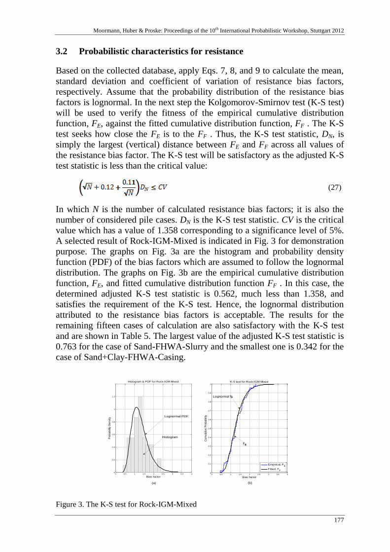
Moormann, Huber & Proske: Proceedings of the 10th International Probabilistic Workshop, Stuttgart 2012
177
3.2 Probabilistic characteristics for resistance
Based on the collected database, apply Eqs. 7, 8, and 9 to calculate the mean,
standard deviation and coefficient of variation of resistance bias factors,
respectively. Assume that the probability distribution of the resistance bias
factors is lognormal. In the next step the Kolgomorov-Smirnov test (K-S test)
will be used to verify the fitness of the empirical cumulative distribution
function, FE, against the fitted cumulative distribution function, FF . The K-S
test seeks how close the FE is to the FF . Thus, the K-S test statistic, DN, is
simply the largest (vertical) distance between FE and FF across all values of
the resistance bias factor. The K-S test will be satisfactory as the adjusted K-S
test statistic is less than the critical value:
(27)
In which N is the number of calculated resistance bias factors; it is also the
number of considered pile cases. DN is the K-S test statistic. CV is the critical
value which has a value of 1.358 corresponding to a significance level of 5%.
A selected result of Rock-IGM-Mixed is indicated in Fig. 3 for demonstration
purpose. The graphs on Fig. 3a are the histogram and probability density
function (PDF) of the bias factors which are assumed to follow the lognormal
distribution. The graphs on Fig. 3b are the empirical cumulative distribution
function, FE, and fitted cumulative distribution function FF . In this case, the
determined adjusted K-S test statistic is 0.562, much less than 1.358, and
satisfies the requirement of the K-S test. Hence, the lognormal distribution
attributed to the resistance bias factors is acceptable. The results for the
remaining fifteen cases of calculation are also satisfactory with the K-S test
and are shown in Table 5. The largest value of the adjusted K-S test statistic is
0.763 for the case of Sand-FHWA-Slurry and the smallest one is 0.342 for the
case of Sand+Clay-FHWA-Casing.
0 0.5 1 1.5 2 2.5 3 3.5 40
0.2
0.4
0.6
0.8
1
1.2
Bias factor
Pro
ba
bili
ty D
en
sity
Histogram & PDF for Rock-IGM-Mixed
0 0.5 1 1.5 2 2.5 3 3.5 40
0.1
0.2
0.3
0.4
0.5
0.6
0.7
0.8
0.9
1
Bias factor
Cu
mu
lativ
e P
rob
ab
ility
K-S test for Rock-IGM-Mixed
Empirical, FE
Fitted, FF
Lognormal PDF
Histogram
(a) (b)
FE
Lognormal FF
Figure 3. The K-S test for Rock-IGM-Mixed
Bach, van Gelder, Bakker & Vrijling: Resistance Factor Calibration of Drilled Shafts for Bridge Foundations
178
Regarding the number of pile cases needed for probability analyses, Fenton
and Griffiths [7] suggested that if sufficient data are available, generally, at
least 20 observations are needed for each dataset. If so, there are nine out of
the sixteen cases of calculation in Table 5 that have a number of pile cases
less than 20. Paikowsky et al. [12] evaluated that one of the major difficulties
with respect to the code calibration is the lack of data. We consider this
problem as a type of uncertainty when using probabilistic analysis methods.
From Table 5, it is easily recognized that the calculation cases with the
sufficient number of pile cases (i.e., from 21 to 46 pile cases) have K-S test
statistics smaller than those of calculation cases with the lack of data (i.e.,
only from 9 to 13 pile cases).
Also, the bias factors, R, represent the difference level between the measured
nominal resistance and the theoretically predicted resistance. If a prediction
method has a bias factor larger than one, that is, this method is an
underpredicted method, and vice versa, a method is overpredicted when its
bias factor is smaller than one. In addition, the coefficient of variation of bias
factors, COVR, is an important parameter which presents a level of uncertainty
in modelling of a prediction method. Therefore, one method which has a bias
factor of one and a coefficient of variation of zero is a perfect prediction
method. In Table 5, the FHWA prediction method for sandy soil and the
casing construction (Sand-FHWA-Casing) is the most underpredicted method
with a bias factor of 2.270. Conversely, the FHWA method used for the
clayey soil and the dry construction (Clay-FHWA-Dry) is the most
overpredicted method with a bias factor of 0.797. Similarly, the RW method
has a coefficient of variation of 0.231 for the sandy+clayey soil and the slurry
construction (Sand+Clay-RW-Slurry), but this method has a coefficient of up
to 0.695 for the sandy soil and the same construction method (Sand-RW-
Slurry). For a prediction method, the values of these parameters will vary in
conjunction with the quantity as well as the quality of the data collected, that
is, the more good data, the more precise the prediction method.
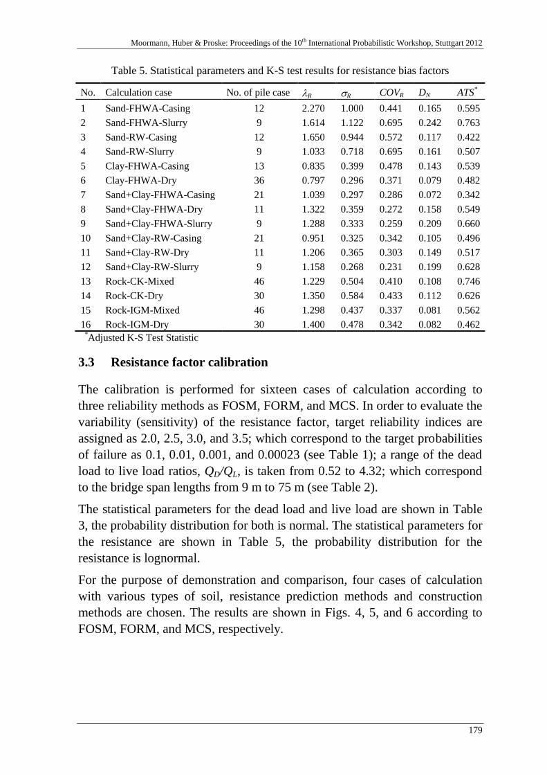
Moormann, Huber & Proske: Proceedings of the 10th International Probabilistic Workshop, Stuttgart 2012
179
Table 5. Statistical parameters and K-S test results for resistance bias factors
No. Calculation case No. of pile case R R COVR DN ATS*
1
2
3
4
5
6
7
8
9
10
11
12
13
14
15
16
Sand-FHWA-Casing
Sand-FHWA-Slurry
Sand-RW-Casing
Sand-RW-Slurry
Clay-FHWA-Casing
Clay-FHWA-Dry
Sand+Clay-FHWA-Casing
Sand+Clay-FHWA-Dry
Sand+Clay-FHWA-Slurry
Sand+Clay-RW-Casing
Sand+Clay-RW-Dry
Sand+Clay-RW-Slurry
Rock-CK-Mixed
Rock-CK-Dry
Rock-IGM-Mixed
Rock-IGM-Dry
12
9
12
9
13
36
21
11
9
21
11
9
46
30
46
30
2.270
1.614
1.650
1.033
0.835
0.797
1.039
1.322
1.288
0.951
1.206
1.158
1.229
1.350
1.298
1.400
1.000
1.122
0.944
0.718
0.399
0.296
0.297
0.359
0.333
0.325
0.365
0.268
0.504
0.584
0.437
0.478
0.441
0.695
0.572
0.695
0.478
0.371
0.286
0.272
0.259
0.342
0.303
0.231
0.410
0.433
0.337
0.342
0.165
0.242
0.117
0.161
0.143
0.079
0.072
0.158
0.209
0.105
0.149
0.199
0.108
0.112
0.081
0.082
0.595
0.763
0.422
0.507
0.539
0.482
0.342
0.549
0.660
0.496
0.517
0.628
0.746
0.626
0.562
0.462 *Adjusted K-S Test Statistic
3.3 Resistance factor calibration
The calibration is performed for sixteen cases of calculation according to
three reliability methods as FOSM, FORM, and MCS. In order to evaluate the
variability (sensitivity) of the resistance factor, target reliability indices are
assigned as 2.0, 2.5, 3.0, and 3.5; which correspond to the target probabilities
of failure as 0.1, 0.01, 0.001, and 0.00023 (see Table 1); a range of the dead
load to live load ratios, QD/QL, is taken from 0.52 to 4.32; which correspond
to the bridge span lengths from 9 m to 75 m (see Table 2).
The statistical parameters for the dead load and live load are shown in Table
3, the probability distribution for both is normal. The statistical parameters for
the resistance are shown in Table 5, the probability distribution for the
resistance is lognormal.
For the purpose of demonstration and comparison, four cases of calculation
with various types of soil, resistance prediction methods and construction
methods are chosen. The results are shown in Figs. 4, 5, and 6 according to
FOSM, FORM, and MCS, respectively.
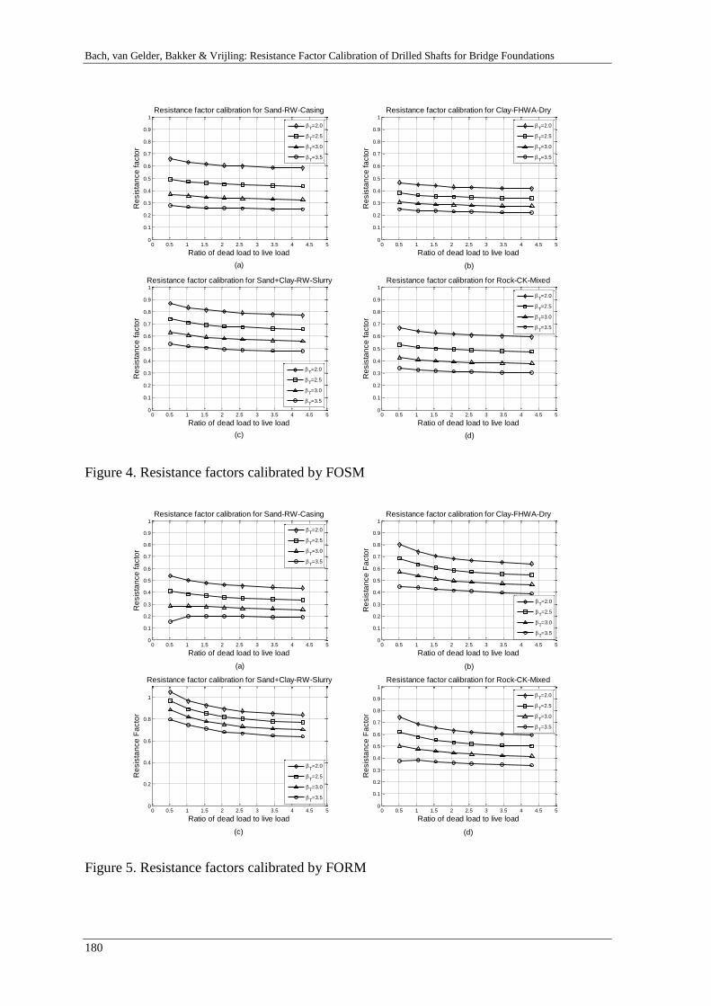
Bach, van Gelder, Bakker & Vrijling: Resistance Factor Calibration of Drilled Shafts for Bridge Foundations
180
0 0.5 1 1.5 2 2.5 3 3.5 4 4.5 50
0.1
0.2
0.3
0.4
0.5
0.6
0.7
0.8
0.9
1
Resistance factor calibration for Sand-RW-Casing
Ratio of dead load to live load
Re
sis
tan
ce
fa
cto
r
T=2.0
T=2.5
T=3.0
T=3.5
0 0.5 1 1.5 2 2.5 3 3.5 4 4.5 50
0.1
0.2
0.3
0.4
0.5
0.6
0.7
0.8
0.9
1
Resistance factor calibration for Clay-FHWA-Dry
Ratio of dead load to live load
Re
sis
tan
ce
fa
cto
r
T=2.0
T=2.5
T=3.0
T=3.5
0 0.5 1 1.5 2 2.5 3 3.5 4 4.5 50
0.1
0.2
0.3
0.4
0.5
0.6
0.7
0.8
0.9
1
Resistance factor calibration for Sand+Clay-RW-Slurry
Ratio of dead load to live load
Re
sis
tan
ce
fa
cto
r
T=2.0
T=2.5
T=3.0
T=3.5
0 0.5 1 1.5 2 2.5 3 3.5 4 4.5 50
0.1
0.2
0.3
0.4
0.5
0.6
0.7
0.8
0.9
1
Resistance factor calibration for Rock-CK-Mixed
Ratio of dead load to live load
Re
sis
tan
ce
fa
cto
r
T=2.0
T=2.5
T=3.0
T=3.5
(a) (b)
(c) (d)
Figure 4. Resistance factors calibrated by FOSM
0 0.5 1 1.5 2 2.5 3 3.5 4 4.5 50
0.1
0.2
0.3
0.4
0.5
0.6
0.7
0.8
0.9
1
Resistance factor calibration for Sand-RW-Casing
Ratio of dead load to live load
Re
sis
tan
ce
fa
cto
r
T=2.0
T=2.5
T=3.0
T=3.5
0 0.5 1 1.5 2 2.5 3 3.5 4 4.5 50
0.1
0.2
0.3
0.4
0.5
0.6
0.7
0.8
0.9
1
Resistance factor calibration for Clay-FHWA-Dry
Ratio of dead load to live load
Re
sis
tan
ce
Fa
cto
r
T=2.0
T=2.5
T=3.0
T=3.5
0 0.5 1 1.5 2 2.5 3 3.5 4 4.5 50
0.2
0.4
0.6
0.8
1
Resistance factor calibration for Sand+Clay-RW-Slurry
Ratio of dead load to live load
Re
sis
tan
ce
Fa
cto
r
T=2.0
T=2.5
T=3.0
T=3.5
0 0.5 1 1.5 2 2.5 3 3.5 4 4.5 50
0.1
0.2
0.3
0.4
0.5
0.6
0.7
0.8
0.9
1
Resistance factor calibration for Rock-CK-Mixed
Ratio of dead load to live load
Re
sis
tan
ce
Fa
cto
r
T=2.0
T=2.5
T=3.0
T=3.5
(a) (b)
(c) (d)
Figure 5. Resistance factors calibrated by FORM
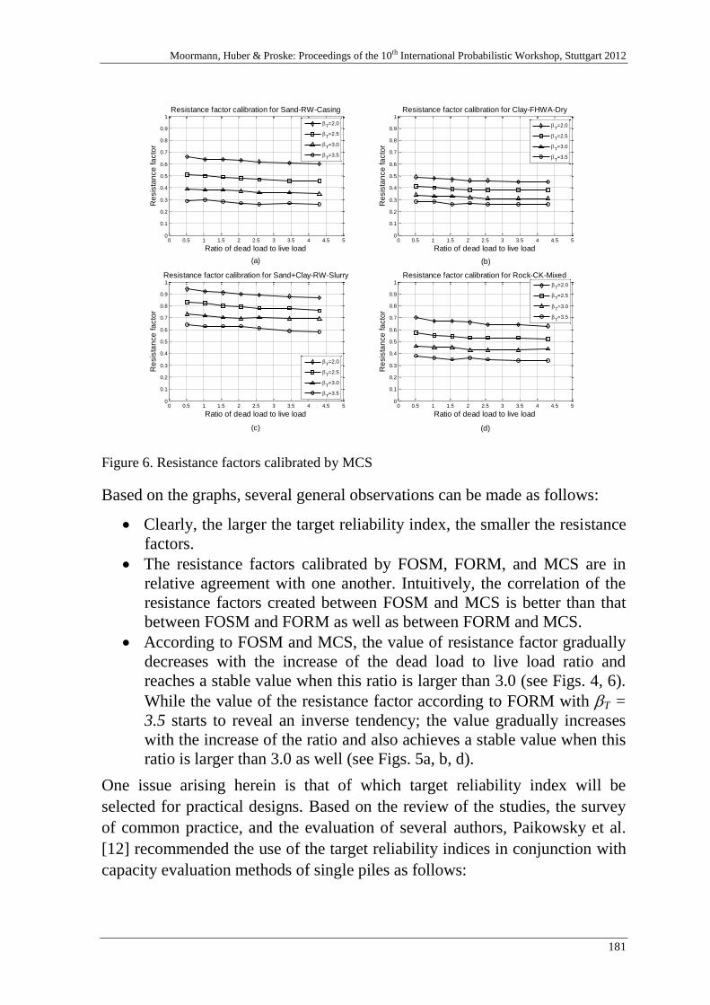
Moormann, Huber & Proske: Proceedings of the 10th International Probabilistic Workshop, Stuttgart 2012
181
0 0.5 1 1.5 2 2.5 3 3.5 4 4.5 50
0.1
0.2
0.3
0.4
0.5
0.6
0.7
0.8
0.9
1
Resistance factor calibration for Sand-RW-Casing
Ratio of dead load to live load
Re
sis
tan
ce
fa
cto
r
T=2.0
T=2.5
T=3.0
T=3.5
0 0.5 1 1.5 2 2.5 3 3.5 4 4.5 50
0.1
0.2
0.3
0.4
0.5
0.6
0.7
0.8
0.9
1
Resistance factor calibration for Clay-FHWA-Dry
Ratio of dead load to live load
Re
sis
tan
ce
fa
cto
r
T=2.0
T=2.5
T=3.0
T=3.5
0 0.5 1 1.5 2 2.5 3 3.5 4 4.5 50
0.1
0.2
0.3
0.4
0.5
0.6
0.7
0.8
0.9
1
Resistance factor calibration for Sand+Clay-RW-Slurry
Ratio of dead load to live load
Re
sis
tan
ce
fa
cto
r
T=2.0
T=2.5
T=3.0
T=3.5
0 0.5 1 1.5 2 2.5 3 3.5 4 4.5 50
0.1
0.2
0.3
0.4
0.5
0.6
0.7
0.8
0.9
1
Resistance factor calibration for Rock-CK-Mixed
Ratio of dead load to live load
Re
sis
tan
ce
fa
cto
r
T=2.0
T=2.5
T=3.0
T=3.5
(a) (b)
(c) (d)
Figure 6. Resistance factors calibrated by MCS
Based on the graphs, several general observations can be made as follows:
Clearly, the larger the target reliability index, the smaller the resistance
factors.
The resistance factors calibrated by FOSM, FORM, and MCS are in
relative agreement with one another. Intuitively, the correlation of the
resistance factors created between FOSM and MCS is better than that
between FOSM and FORM as well as between FORM and MCS.
According to FOSM and MCS, the value of resistance factor gradually
decreases with the increase of the dead load to live load ratio and
reaches a stable value when this ratio is larger than 3.0 (see Figs. 4, 6).
While the value of the resistance factor according to FORM with T =
3.5 starts to reveal an inverse tendency; the value gradually increases
with the increase of the ratio and also achieves a stable value when this
ratio is larger than 3.0 as well (see Figs. 5a, b, d).
One issue arising herein is that of which target reliability index will be
selected for practical designs. Based on the review of the studies, the survey
of common practice, and the evaluation of several authors, Paikowsky et al.
[12] recommended the use of the target reliability indices in conjunction with
capacity evaluation methods of single piles as follows:
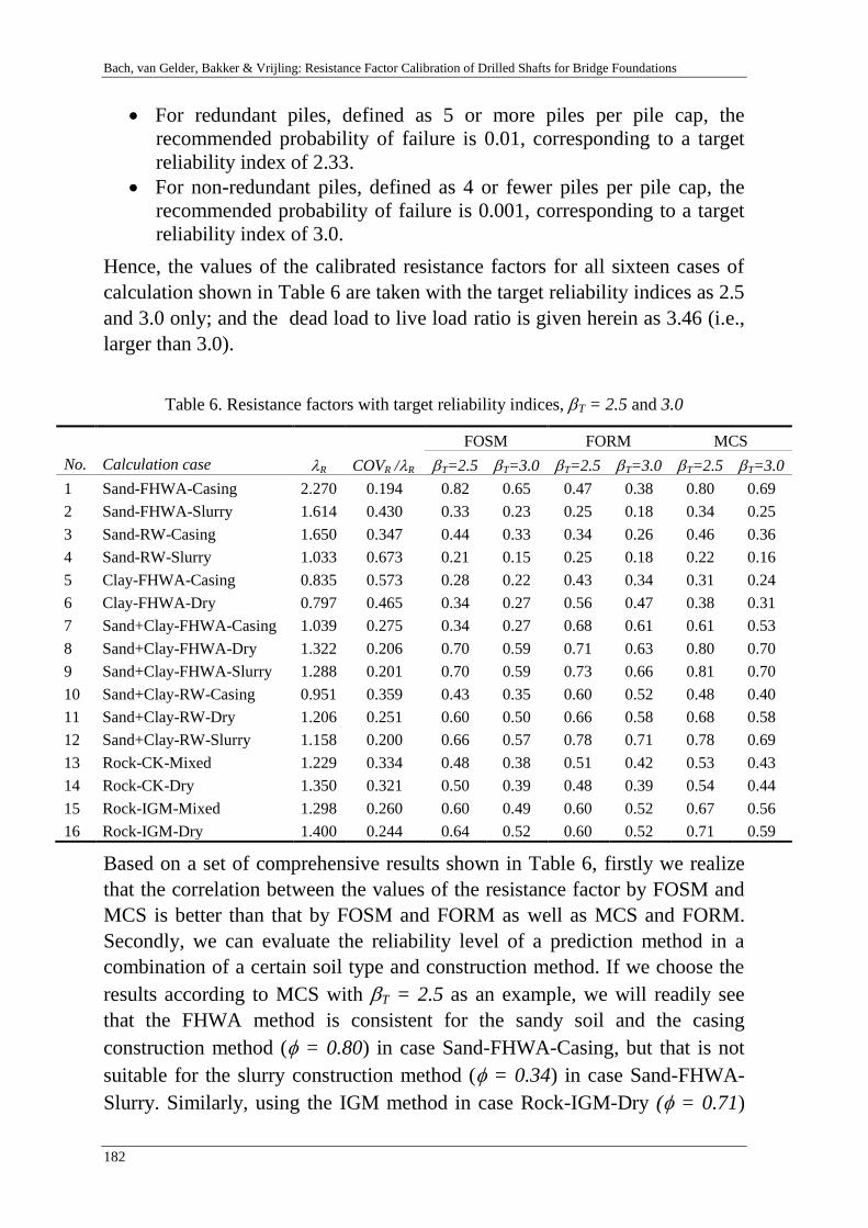
Bach, van Gelder, Bakker & Vrijling: Resistance Factor Calibration of Drilled Shafts for Bridge Foundations
182
For redundant piles, defined as 5 or more piles per pile cap, the
recommended probability of failure is 0.01, corresponding to a target
reliability index of 2.33.
For non-redundant piles, defined as 4 or fewer piles per pile cap, the
recommended probability of failure is 0.001, corresponding to a target
reliability index of 3.0.
Hence, the values of the calibrated resistance factors for all sixteen cases of
calculation shown in Table 6 are taken with the target reliability indices as 2.5
and 3.0 only; and the dead load to live load ratio is given herein as 3.46 (i.e.,
larger than 3.0).
Table 6. Resistance factors with target reliability indices, T = 2.5 and 3.0
FOSM FORM MCS
No. Calculation case R COVR /R T=2.5 T=3.0 T=2.5 T=3.0 T=2.5 T=3.0
1
2
3
4
5
6
7
8
9
10
11
12
13
14
15
16
Sand-FHWA-Casing
Sand-FHWA-Slurry
Sand-RW-Casing
Sand-RW-Slurry
Clay-FHWA-Casing
Clay-FHWA-Dry
Sand+Clay-FHWA-Casing
Sand+Clay-FHWA-Dry
Sand+Clay-FHWA-Slurry
Sand+Clay-RW-Casing
Sand+Clay-RW-Dry
Sand+Clay-RW-Slurry
Rock-CK-Mixed
Rock-CK-Dry
Rock-IGM-Mixed
Rock-IGM-Dry
2.270
1.614
1.650
1.033
0.835
0.797
1.039
1.322
1.288
0.951
1.206
1.158
1.229
1.350
1.298
1.400
0.194
0.430
0.347
0.673
0.573
0.465
0.275
0.206
0.201
0.359
0.251
0.200
0.334
0.321
0.260
0.244
0.82
0.33
0.44
0.21
0.28
0.34
0.34
0.70
0.70
0.43
0.60
0.66
0.48
0.50
0.60
0.64
0.65
0.23
0.33
0.15
0.22
0.27
0.27
0.59
0.59
0.35
0.50
0.57
0.38
0.39
0.49
0.52
0.47
0.25
0.34
0.25
0.43
0.56
0.68
0.71
0.73
0.60
0.66
0.78
0.51
0.48
0.60
0.60
0.38
0.18
0.26
0.18
0.34
0.47
0.61
0.63
0.66
0.52
0.58
0.71
0.42
0.39
0.52
0.52
0.80
0.34
0.46
0.22
0.31
0.38
0.61
0.80
0.81
0.48
0.68
0.78
0.53
0.54
0.67
0.71
0.69
0.25
0.36
0.16
0.24
0.31
0.53
0.70
0.70
0.40
0.58
0.69
0.43
0.44
0.56
0.59
Based on a set of comprehensive results shown in Table 6, firstly we realize
that the correlation between the values of the resistance factor by FOSM and
MCS is better than that by FOSM and FORM as well as MCS and FORM.
Secondly, we can evaluate the reliability level of a prediction method in a
combination of a certain soil type and construction method. If we choose the
results according to MCS with T = 2.5 as an example, we will readily see
that the FHWA method is consistent for the sandy soil and the casing
construction method ( = 0.80) in case Sand-FHWA-Casing, but that is not
suitable for the slurry construction method ( = 0.34) in case Sand-FHWA-
Slurry. Similarly, using the IGM method in case Rock-IGM-Dry ( = 0.71)
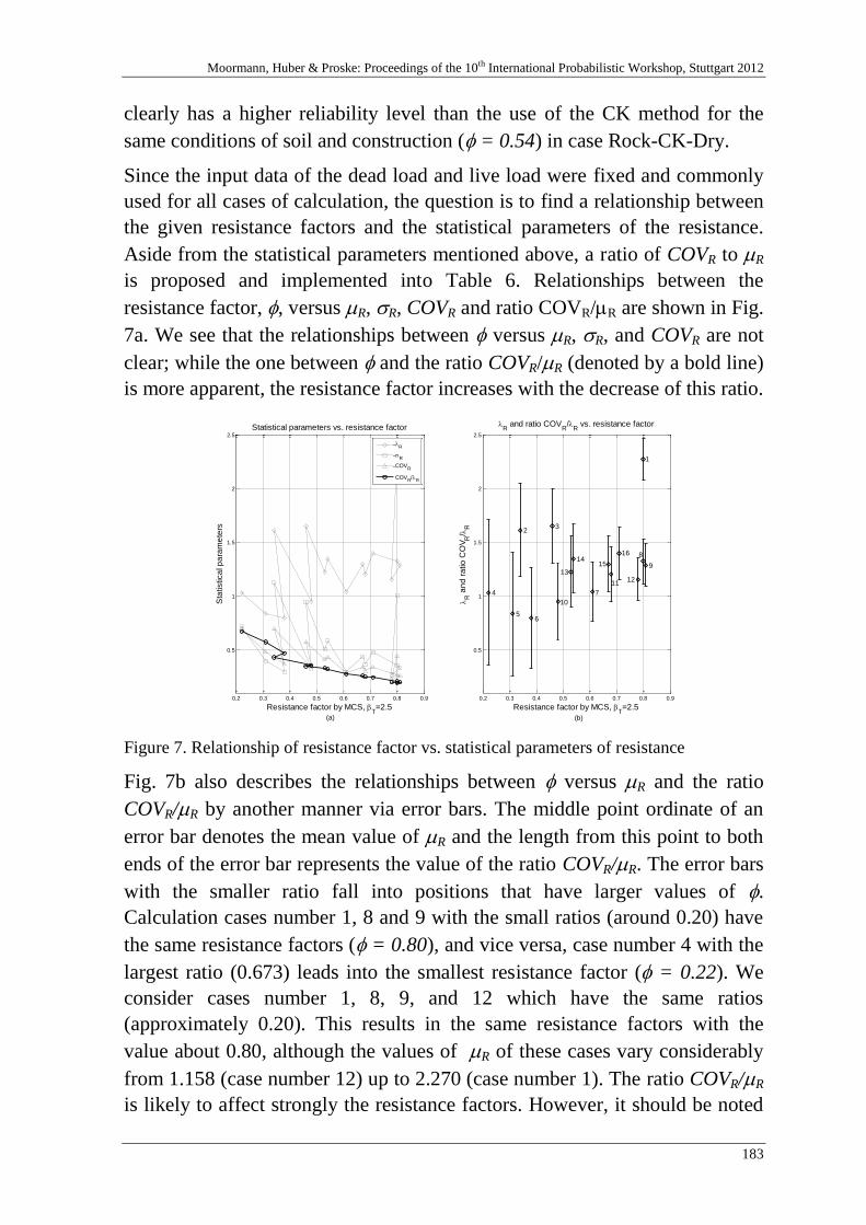
Moormann, Huber & Proske: Proceedings of the 10th International Probabilistic Workshop, Stuttgart 2012
183
clearly has a higher reliability level than the use of the CK method for the
same conditions of soil and construction ( = 0.54) in case Rock-CK-Dry.
Since the input data of the dead load and live load were fixed and commonly
used for all cases of calculation, the question is to find a relationship between
the given resistance factors and the statistical parameters of the resistance.
Aside from the statistical parameters mentioned above, a ratio of COVR to R
is proposed and implemented into Table 6. Relationships between the
resistance factor, , versus R, R, COVR and ratio COVR/R are shown in Fig.
7a. We see that the relationships between versus R, R, and COVR are not
clear; while the one between and the ratio COVR/R (denoted by a bold line)
is more apparent, the resistance factor increases with the decrease of this ratio.
0.2 0.3 0.4 0.5 0.6 0.7 0.8 0.9
0.5
1
1.5
2
2.5
Statistical parameters vs. resistance factor
Resistance factor by MCS, T=2.5
Sta
tistica
l p
ara
me
ters
R
R
COVR
COVR/
R
0.2 0.3 0.4 0.5 0.6 0.7 0.8 0.9
0.5
1
1.5
2
2.5
R
and ratio COVR
/R
vs. resistance factor
Resistance factor by MCS, T=2.5
R
an
d r
atio
CO
VR
/ R
(a) (b)
1
23
4
56
7
8
9
10
1112
13
1415
16
Figure 7. Relationship of resistance factor vs. statistical parameters of resistance
Fig. 7b also describes the relationships between versus R and the ratio
COVR/R by another manner via error bars. The middle point ordinate of an
error bar denotes the mean value of R and the length from this point to both
ends of the error bar represents the value of the ratio COVR/R. The error bars
with the smaller ratio fall into positions that have larger values of .
Calculation cases number 1, 8 and 9 with the small ratios (around 0.20) have
the same resistance factors ( = 0.80), and vice versa, case number 4 with the
largest ratio (0.673) leads into the smallest resistance factor ( = 0.22). We
consider cases number 1, 8, 9, and 12 which have the same ratios
(approximately 0.20). This results in the same resistance factors with the
value about 0.80, although the values of R of these cases vary considerably
from 1.158 (case number 12) up to 2.270 (case number 1). The ratio COVR/R
is likely to affect strongly the resistance factors. However, it should be noted
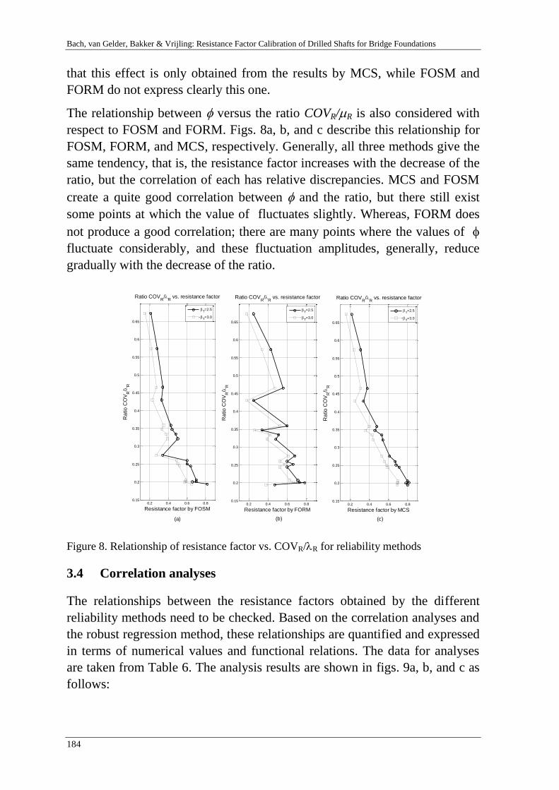
Bach, van Gelder, Bakker & Vrijling: Resistance Factor Calibration of Drilled Shafts for Bridge Foundations
184
that this effect is only obtained from the results by MCS, while FOSM and
FORM do not express clearly this one.
The relationship between versus the ratio COVR/R is also considered with
respect to FOSM and FORM. Figs. 8a, b, and c describe this relationship for
FOSM, FORM, and MCS, respectively. Generally, all three methods give the
same tendency, that is, the resistance factor increases with the decrease of the
ratio, but the correlation of each has relative discrepancies. MCS and FOSM
create a quite good correlation between and the ratio, but there still exist
some points at which the value of fluctuates slightly. Whereas, FORM does
not produce a good correlation; there are many points where the values of
fluctuate considerably, and these fluctuation amplitudes, generally, reduce
gradually with the decrease of the ratio.
0.2 0.4 0.6 0.80.15
0.2
0.25
0.3
0.35
0.4
0.45
0.5
0.55
0.6
0.65
Ratio COVR
/R
vs. resistance factor
Resistance factor by FOSM
Ra
tio
CO
VR
/ R
T=2.5
T=3.0
0.2 0.4 0.6 0.80.15
0.2
0.25
0.3
0.35
0.4
0.45
0.5
0.55
0.6
0.65
Ratio COVR
/R
vs. resistance factor
Resistance factor by FORM
Ra
tio
CO
VR
/ R
T=2.5
T=3.0
0.2 0.4 0.6 0.80.15
0.2
0.25
0.3
0.35
0.4
0.45
0.5
0.55
0.6
0.65
Ratio COVR
/R
vs. resistance factor
Resistance factor by MCS
Ra
tio
CO
VR
/ R
T=2.5
T=3.0
(a) (b) (c)
Figure 8. Relationship of resistance factor vs. COVR/R for reliability methods
3.4 Correlation analyses
The relationships between the resistance factors obtained by the different
reliability methods need to be checked. Based on the correlation analyses and
the robust regression method, these relationships are quantified and expressed
in terms of numerical values and functional relations. The data for analyses
are taken from Table 6. The analysis results are shown in figs. 9a, b, and c as
follows:
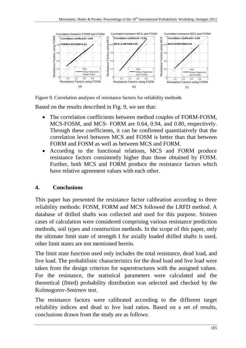
Moormann, Huber & Proske: Proceedings of the 10th International Probabilistic Workshop, Stuttgart 2012
185
0 0.2 0.4 0.6 0.8 10
0.2
0.4
0.6
0.8
1
Resistance Factors using FOSM
Re
sis
tan
ce
Fa
cto
rs u
sin
g F
OR
M
Correlation between FORM and FOSM
Data
Robust Regression
FORM=FOSM
0 0.2 0.4 0.6 0.8 10
0.2
0.4
0.6
0.8
1
Resistance Factors using FOSM
Re
sis
tan
ce
Fa
cto
rs u
sin
g M
CS
Correlation between MCS and FOSM
Data
Robust Regression
MCS=FOSM
0 0.2 0.4 0.6 0.8 10
0.2
0.4
0.6
0.8
1
Resistance Factors using FORM
Re
sis
tan
ce
Fa
cto
rs u
sin
g M
CS
Correlation between MCS and FORM
Data
Robust Regression
MCS=FORM
(a) (c)(b)
Correlation coefficient = 0.64
FORM=0.81FOSM+0.14
Correlation coefficient = 0.94
MCS=1.18FOSM-0.02
Correlation coefficient = 0.80
MCS=0.95FOSM+0.04
Figure 9. Correlation analyses of resistance factors for reliability methods
Based on the results described in Fig. 9, we see that:
The correlation coefficients between method couples of FORM-FOSM,
MCS-FOSM, and MCS- FORM are 0.64, 0.94, and 0.80, respectively.
Through these coefficients, it can be confirmed quantitatively that the
correlation level between MCS and FOSM is better than that between
FORM and FOSM as well as between MCS and FORM.
According to the functional relations, MCS and FORM produce
resistance factors consistently higher than those obtained by FOSM.
Further, both MCS and FORM produce the resistance factors which
have relative agreement values with each other.
4. Conclusions
This paper has presented the resistance factor calibration according to three
reliability methods: FOSM, FORM and MCS followed the LRFD method. A
database of drilled shafts was collected and used for this purpose. Sixteen
cases of calculation were considered comprising various resistance prediction
methods, soil types and construction methods. In the scope of this paper, only
the ultimate limit state of strength I for axially loaded drilled shafts is used,
other limit states are not mentioned herein.
The limit state function used only includes the total resistance, dead load, and
live load. The probabilistic characteristics for the dead load and live load were
taken from the design criterion for superstructures with the assigned values.
For the resistance, the statistical parameters were calculated and the
theoretical (fitted) probability distribution was selected and checked by the
Kolmogorov-Smirnov test.
The resistance factors were calibrated according to the different target
reliability indices and dead to live load ratios. Based on a set of results,
conclusions drawn from the study are as follows:
Bach, van Gelder, Bakker & Vrijling: Resistance Factor Calibration of Drilled Shafts for Bridge Foundations
186
1. A larger target reliability index results in smaller resistance factors.
2. The value of the resistance factor decreases gradually with the increase
of the dead to live load ratio and reaches a stable value when this ratio
is larger than 3.0. However, there was a discrepancy with respect to
FORM, when the target reliability index is larger than 3.5, then the
value of resistance factor increases gradually with the increase of the
ratio and also reaches a stable value as this ratio is also larger than 3.0.
3. Through Table 6, a design engineer can choose a prediction method
that has a consistent reliability level with respect to a prescribed soil
condition and a specified construction method.
4. The value of the resistance factor increases gradually with the decrease
of the ratio of the coefficient of variation to the mean of the resistance
bias factor. In this study, MCS was used to derive this observation.
5. MCS and FORM produce resistance factors consistently higher than
those obtained by FOSM. With regard to the correlations between the
methods, MCS and FOSM have a good correlation with a correlation
coefficient of 0.94.
6. MCS has indicated to be a powerful and confident tool aiming to solve
probabilistic problems in civil engineering.
ACKNOWLEDGEMENTS
This study is mainly funded by Project 322 of the Vietnam Ministry of
Education and Training and partly supported by CICAT and the Section of
Hydraulic Engineering, Delft University of Technology, the Netherlands.
REFERENCES
[1] Abu-Farsakh, M. Y.; and Yu, X.: Interpretation criteria to evaluate resistance
factors for axial load capacity of drilled shafts. Transportation Research Record:
Journal of the Transportation Research Board, 2202(1), 20-31. (2010)
[2] Allen, T. M.; Nowak, A. S.; and Bathurst, R. J.: Transportation research circular E-
C079: Calibration to determine load and resistance factors for geotechnical and
structural design. Technical report, Transportation Research Board, Foundations of
Bridges and Other Structures Committee, General Structures Committee. 2005.
Washington, D.C.
[3] Ang, A. H.-S.; and Tang, W. H.: Probability Concepts in Engineering Planning and
Design-Decision Risk and Reliability. Volume II. John Wiley and Sons, 1984

Moormann, Huber & Proske: Proceedings of the 10th International Probabilistic Workshop, Stuttgart 2012
187
[4] Ayyub, B. M.; Assakkaf, I. I.; and Atua, K.: Reliability-based load and resistance
factor design (LRFD) of hull girders for surface ships. Naval Engineers Journal,
112(4), 279-296. (2000)
[5] Barker, R. M.; Duncan, J. M.; Rojiani, K. B.; Ooi, P. S. K.; Tan, C. K.; and Kim, S.
G.: National cooperative highway research program - Report 343: Manuals for the
design of bridge foundations. Technical report, Transportation Research Board,
National Research Council. 1991. Washington, D. C.
[6] Brown, D. A.; Turner, J. P.; and Castelli, R. J.: Federal highway adminitration -
Report No. FHWA-NHI-10-016: Drilled shafts: Construction procedures and LRFD
design methods. Technical report, National Highway Institute, Federal Highway
Administration, US Department of Transportation. 2010. Washington, D.C.
[7] Fenton, G. A.; and Griffiths, D. V.: Risk Assessment in Geotechnical Engineering.
John Wiley and Sons, 2008
[8] Hansell, W. C.; and Viest, I. M.: Load factor design for steel highway bridges. AISC
Engineering Journal, 8(4), 113-123. (1971)
[9] Hasofer, A. M.; and Lind, N. C.: An exact and invariant first-order reliability format.
Journal of Engineering Mechanics, 100(EM1), 111-121. (1974)
[10] Nowak, A. S.: National cooperative highway research program - Report 368:
Calibration of LRFD bridge design code. Technical report, Transportation Research
Board. 1999. Washington, D. C.
[11] O'Neill, M. W.; and Reese, L. C.: Federal highway administration - Report No.
FHWA-IF-99-025: Drilled shafts: Construction procedures and design methods.
Technical report, Federal Highway Administration. 1999. Washington, D.C.
[12] Paikowsky, S. G.; Birgisson, B.; McVay, M.; Nguyen, T.; Kuo, C.; Baecher, G. B.;
Ayyub, B. M.; Stenersen, K.; O'Malley, K.; Chernauskas, L.; and O'Neill, M.:
National cooperative highway research program - Report 507: Load and resistance
factor design (LRFD) for deep foundations. Technical report, Transportation
Research Board. 2004. Washington, D. C.
[13] Withiam, J.; Voytko, E.; Barker, R.; Duncan, J.; Kelly, B.; Musser, S.; and Elias, V.:
Federal highway administration - Publication No. FHWA-HI-98-032: Load and
resistance factor design (LRFD) for highway bridge substructures. Technical report,
National Highway Institute, Federal Highway Administration, US Department of
Transportation. 1998. Washington, D.C.

Bach, van Gelder, Bakker & Vrijling: Resistance Factor Calibration of Drilled Shafts for Bridge Foundations
188
Moormann, Huber & Proske: Proceedings of the 10th International Probabilistic Workshop, Stuttgart 2012
189
Reliability and Risk Analysis of Concrete
Bridges for Hazard Scenarios
Vazul Boros, Balthasar Novák
Institute for Lightweight Structures and Conceptual Design,
University of Stuttgart
Abstract: Bridges are essential, yet also vulnerable parts of the infrastructure.
They are subject to natural disasters, traffic accidents and terrorist attacks,
moreover they generally require significant resources and time to be repaired
or replaced. In this research critical reinforced and prestressed concrete bridges
were to be identified. Based on a complex probabilistic model the reliability
index was assessed for several hazard scenarios considering four different traf-
fic scenarios. An approximation by the Monte Carlo method forms the core of
the reliability analysis, however the variance of the approximation can be re-
duced effectively, by considering the model uncertainty factors analytically.
The introduced method is demonstrated on the example of two representative
bridges with five hazard scenarios. Based on the results of the Monte Carlo
method an approximation of the reliability index, considering also the addi-
tional safety due to the redistribution of moments in statically indeterminate
structures, is presented. The Monte Carlo method also enables the risk analysis
of the different hazard scenarios, taking into account the consequences of fail-
ure. These results provide valuable tools for proprietors and operators of traffic
infrastructure to reach important ethical and economic decisions. Some inter-
esting insights of the research on the combination of different time-dependent
actions and the assessment of the reliability index of systems with several cor-
related limit states are shown.
1 Introduction
The highway network plays an essential part in a country’s economy and so-
cial life. Its continuous and undisrupted operation is vital for our society. The
probably most vulnerable components of the road infrastructure are bridges
Boros & Novak: Reliability and Risk Analysis of Concrete Bridges for Hazard Scenarios
190
and tunnels. These structures not only act as bottle-necks in the highway sys-
tem, but also have to face a number of different hazards. Bridges can be af-
fected by vehicle impact against vital structural components such as cables or
pillars. Due to the rising percentage of heavy traffic and growing average ve-
hicle weight these impact loads have to be revised regularly. The effect of
climate change on structures has to be taken into account, too. It results in
higher wind velocities, increased temperatures and rainfall, thus causing
storms, floods and other natural disasters. Finally, another ever greater threat
to important infrastructure components is represented by terrorist attacks.
The aim of the German research project "Protection of Critical Bridges and
Tunnels in a Road Network" (SKRIBT in German) was, to investigate the ef-
fects of these hazard scenarios on bridges and tunnels and to develop effective
protection measures and strategies as described in [1]. The objective was to
rank different types of structures according to their criticality and thus enable
traffic administrations to identify their most vulnerable structures. Subse-
quently, suitable protection measures had to be identified and their effect on
the criticality of the structure had to be assessed.
The objectives of the research project required the assessment of the criticali-
ty of a structure-hazard combination with suitable indicators. This is also es-
sential for the examination of protection measures, as the reduction of
criticality due to a protection measure describes its efficiency. Three main
aspects have been considered regarding the criticality of a structure: effects on
road users, influence on the road network and structural aspects. All three
main aspects have been investigated in detail in the research project, yet this
paper addresses the assessment of the criticality of the structure, in particular
of reinforced and prestressed concrete bridges.
2 Probabilistic model
The probabilistic model is based on the traditional separation of actions and
resistances common to structural engineering. After careful considerations
and extensive literature review basic variables have been selected for both
sides.
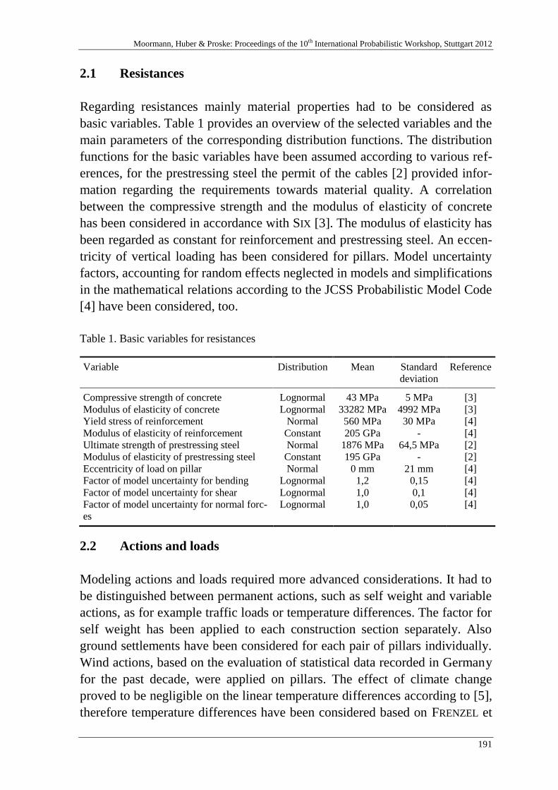
Moormann, Huber & Proske: Proceedings of the 10th International Probabilistic Workshop, Stuttgart 2012
191
2.1 Resistances
Regarding resistances mainly material properties had to be considered as
basic variables. Table 1 provides an overview of the selected variables and the
main parameters of the corresponding distribution functions. The distribution
functions for the basic variables have been assumed according to various ref-
erences, for the prestressing steel the permit of the cables [2] provided infor-
mation regarding the requirements towards material quality. A correlation
between the compressive strength and the modulus of elasticity of concrete
has been considered in accordance with SIX [3]. The modulus of elasticity has
been regarded as constant for reinforcement and prestressing steel. An eccen-
tricity of vertical loading has been considered for pillars. Model uncertainty
factors, accounting for random effects neglected in models and simplifications
in the mathematical relations according to the JCSS Probabilistic Model Code
[4] have been considered, too.
Table 1. Basic variables for resistances
Variable Distribution Mean Standard
deviation
Reference
Compressive strength of concrete
Modulus of elasticity of concrete
Yield stress of reinforcement
Modulus of elasticity of reinforcement
Ultimate strength of prestressing steel
Modulus of elasticity of prestressing steel
Eccentricity of load on pillar
Factor of model uncertainty for bending
Factor of model uncertainty for shear
Factor of model uncertainty for normal forc-
es
Lognormal
Lognormal
Normal
Constant
Normal
Constant
Normal
Lognormal
Lognormal
Lognormal
43 MPa
33282 MPa
560 MPa
205 GPa
1876 MPa
195 GPa
0 mm
1,2
1,0
1,0
5 MPa
4992 MPa
30 MPa
-
64,5 MPa
-
21 mm
0,15
0,1
0,05
[3]
[3]
[4]
[4]
[2]
[2]
[4]
[4]
[4]
[4]
2.2 Actions and loads
Modeling actions and loads required more advanced considerations. It had to
be distinguished between permanent actions, such as self weight and variable
actions, as for example traffic loads or temperature differences. The factor for
self weight has been applied to each construction section separately. Also
ground settlements have been considered for each pair of pillars individually.
Wind actions, based on the evaluation of statistical data recorded in Germany
for the past decade, were applied on pillars. The effect of climate change
proved to be negligible on the linear temperature differences according to [5],
therefore temperature differences have been considered based on FRENZEL et
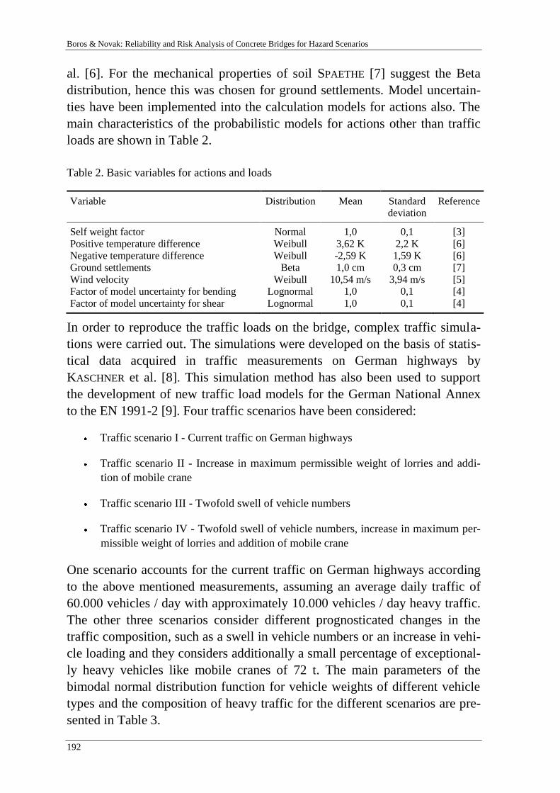
Boros & Novak: Reliability and Risk Analysis of Concrete Bridges for Hazard Scenarios
192
al. [6]. For the mechanical properties of soil SPAETHE [7] suggest the Beta
distribution, hence this was chosen for ground settlements. Model uncertain-
ties have been implemented into the calculation models for actions also. The
main characteristics of the probabilistic models for actions other than traffic
loads are shown in Table 2.
Table 2. Basic variables for actions and loads
Variable Distribution Mean Standard
deviation
Reference
Self weight factor
Positive temperature difference
Negative temperature difference
Ground settlements
Wind velocity
Factor of model uncertainty for bending
Factor of model uncertainty for shear
Normal
Weibull
Weibull
Beta
Weibull
Lognormal
Lognormal
1,0
3,62 K
-2,59 K
1,0 cm
10,54 m/s
1,0
1,0
0,1
2,2 K
1,59 K
0,3 cm
3,94 m/s
0,1
0,1
[3]
[6]
[6]
[7]
[5]
[4]
[4]
In order to reproduce the traffic loads on the bridge, complex traffic simula-
tions were carried out. The simulations were developed on the basis of statis-
tical data acquired in traffic measurements on German highways by
KASCHNER et al. [8]. This simulation method has also been used to support
the development of new traffic load models for the German National Annex
to the EN 1991-2 [9]. Four traffic scenarios have been considered:
Traffic scenario I - Current traffic on German highways
Traffic scenario II - Increase in maximum permissible weight of lorries and addi-
tion of mobile crane
Traffic scenario III - Twofold swell of vehicle numbers
Traffic scenario IV - Twofold swell of vehicle numbers, increase in maximum per-
missible weight of lorries and addition of mobile crane
One scenario accounts for the current traffic on German highways according
to the above mentioned measurements, assuming an average daily traffic of
60.000 vehicles / day with approximately 10.000 vehicles / day heavy traffic.
The other three scenarios consider different prognosticated changes in the
traffic composition, such as a swell in vehicle numbers or an increase in vehi-
cle loading and they considers additionally a small percentage of exceptional-
ly heavy vehicles like mobile cranes of 72 t. The main parameters of the
bimodal normal distribution function for vehicle weights of different vehicle
types and the composition of heavy traffic for the different scenarios are pre-
sented in Table 3.

Moormann, Huber & Proske: Proceedings of the 10th International Probabilistic Workshop, Stuttgart 2012
193
Table 3. Parameters of basic variables for vehicle weights and traffic composition
Vehicle type Portion
(%)
Mean
(kN)
Standard
deviation
(kN)
Portion
(%)
Mean
(kN)
Standard
deviation
(kN)
I/III
Share
(%)
II/IV
Share
(%)
Type 8
Type 33
Type 41
Type 97
Type 98
Type 98 (modified)
Mobile crane
49
20
69
34
62
62
100
59,6
190,3
276,8
156,7
259,6
259,6
720,0
14,6
23,2
59,5
18,8
92,0
92,0
63,3
51
80
31
66
38
38
-
91,7
208,4
414,5
211,4
405,3
526,9
-
44,0
73,9
32,5
52,8
24,8
24,8
-
11,0
5,0
17,0
8,0
59,0
-
-
10,9
4,9
16,9
7,9
-
58,9
0,5
Additional basic variables for the traffic simulations included the distance be-
tween vehicles and probabilities for simulating traffic congestion on the
bridge. The distance between the axles for each vehicle type and the distribu-
tion of loads on the axles have been regarded as constant. The different vehi-
cle types with the distances between axles are presented in Figure 1.
(a) Vehicle Type 8 (b) Vehicle type 33
(c) Vehicle Type 41 (d) Vehicle type 97
(e) Vehicle Type 98 (f) Mobile crane
Figure 1. Vehicle types with distances between axles
3 Reliability analysis
3.1 Method of model uncertainties
The Monte Carlo method has been implemented to determine the risk and re-
liability indicators in question. In order to improve the accuracy of the Monte
Boros & Novak: Reliability and Risk Analysis of Concrete Bridges for Hazard Scenarios
194
Carlo simulation a special method considering the model uncertainties, has
been developed. The technique is similar to the importance sampling method,
which utilizes prior information about which domain of the possible values of
basic variables contributes most to the probability of failure, and achieves a
variance reduction by centering the simulation on this area as described in
FABER [10]. In an analogous way the applied method considers only those
values of the model uncertainties which result in the failure of the structure.
For each of the basic variables, with the exception of model uncertainties, n
different possible realizations according to the corresponding population func-
tion are generated. Thereafter the resistance and action forces can be calculat-
ed for each of these realizations. The limit state function for one realization
can be stated as
0EiRi
ER (1)
with i
R resistance forces for the .i simulation
iE action forces for the .i simulation
R model uncertainty factor for resistances
E model uncertainty factor for actions
The model uncertainty factors follow the logarithmic normal distribution,
therefore they can be substituted by the exponents of normally distributed var-
iables R
U and E
U .
0ER U
i
U
ieEeR (2)
i
iUU
R
Ee ER (3)
As the exponential function is strictly increasing, the inequality has to be also
valid for the natural logarithm of both sides.
i
i
ERR
EUU ln (4)
The variables RU and EU being normally distributed, their difference has to
be normally distributed also. Therefore the probability of the limit state func-
tion not being fulfilled can be calculated as the value of this normal distribu-
tion at ii
REln . The corresponding probability of failure for this realization
of basic variables can then expressed as
Moormann, Huber & Proske: Proceedings of the 10th International Probabilistic Workshop, Stuttgart 2012
195
22
ln
ˆ
ER
ER
UU
UU
i
i
if
R
E
P (5)
with if
P probability of failure for the .i simulation
x standard normal distribution function
RU mean value of variable RU
EU mean value of variable EU
RU
standard deviation of variable RU
EU
standard deviation of variable EU
By this equation each realization in the simulation provides an estimate of the
failure probability for the investigated limit state. The overall failure probabil-
ity considering all n simulations can be expressed as
n
iiff
Pn
P1
ˆ1ˆ (6)
The variance of the failure probability can then be calculated in analogy to the
importance sampling technique by
f
n
iiff
PPnn
PVar ˆˆ1
1
1ˆ1
2 (7)
In comparison the variance of the crude Monte Carlo method can be estimated
according to RACKWITZ [11] by
ff
ff
f
PnPn
PPnPVar
ˆ
1
ˆ
ˆ1ˆˆ (8)
In both cases the variance is dependent on the number of simulations and the
probability of failure which of course can also be expressed by the reliability
index. In Figure 2 the variances obtained by the method of model uncertain-
ties for different limit states and the variance of the crude Monte Carlo meth-
od according to Equation (8) are plotted.
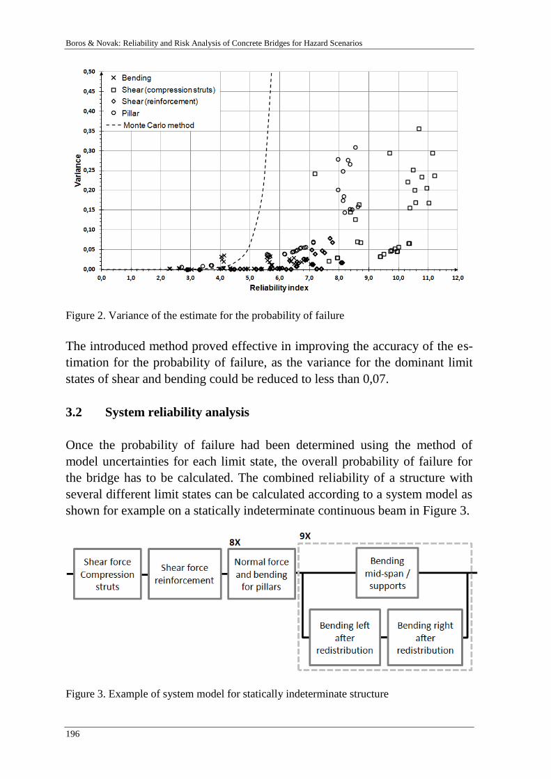
Boros & Novak: Reliability and Risk Analysis of Concrete Bridges for Hazard Scenarios
196
Figure 2. Variance of the estimate for the probability of failure
The introduced method proved effective in improving the accuracy of the es-
timation for the probability of failure, as the variance for the dominant limit
states of shear and bending could be reduced to less than 0,07.
3.2 System reliability analysis
Once the probability of failure had been determined using the method of
model uncertainties for each limit state, the overall probability of failure for
the bridge has to be calculated. The combined reliability of a structure with
several different limit states can be calculated according to a system model as
shown for example on a statically indeterminate continuous beam in Figure 3.
Figure 3. Example of system model for statically indeterminate structure

Moormann, Huber & Proske: Proceedings of the 10th International Probabilistic Workshop, Stuttgart 2012
197
The different failure modes are to be considered as series systems, as exceed-
ing any of the limit states would result in failure. The redistribution of mo-
ments in the statically indeterminate structure can be modeled by a parallel
system, as the failure of one cross-section due to bending does not result in a
system failure, provided that both neighboring cross-sections can take the ad-
ditional loads after redistribution.
The JCSS Probabilistic Model Code [4] provides recommendations for first-
order approximations and first-order reliability bounds for series and parallel
systems. The first-order approximation for series systems is given by
;1mfsys
P (9)
with m
multi-variate standard normal distribution function
vector of component reliability indices
correlation matrix between safety margins
The upper bound for series systems is
1;jfsys
PMinP (10)
with j
P failure probability of the .j component
In analogy the first-order approximation for parallel systems is given by
;mfsys
P (11)
The upper bound for parallel systems is
jfsysPMinP (12)
In order to asses the accuracy of these upper bounds the difference between
the first-order approximation and the upper bound has been investigated on a
simple system with two components. For the two components equal reliability
indices were assumed. This reliability index was varied in the range of 1 to 6
and the difference between the upper bound and the first-order approximation
has been calculated for seven different correlation coefficients both for series
and parallel systems. The results are shown in Figure 4.
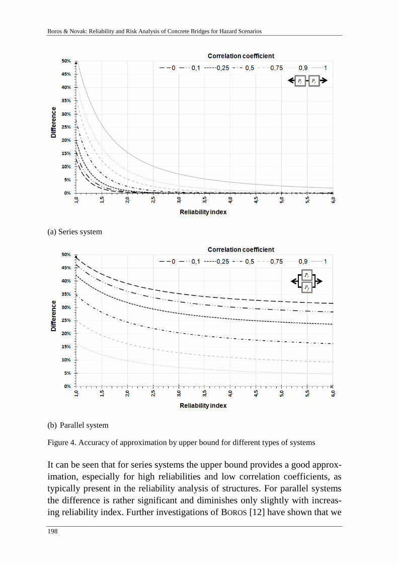
Boros & Novak: Reliability and Risk Analysis of Concrete Bridges for Hazard Scenarios
198
(a) Series system
(b) Parallel system
Figure 4. Accuracy of approximation by upper bound for different types of systems
It can be seen that for series systems the upper bound provides a good approx-
imation, especially for high reliabilities and low correlation coefficients, as
typically present in the reliability analysis of structures. For parallel systems
the difference is rather significant and diminishes only slightly with increas-
ing reliability index. Further investigations of BOROS [12] have shown that we
Moormann, Huber & Proske: Proceedings of the 10th International Probabilistic Workshop, Stuttgart 2012
199
can obtain similar results even if the two components have different failure
probabilities. Therefore we can conclude that for series systems the upper
bound provides acceptable results, however for parallel systems disregarding
the correlations by using the upper bound may results in considerable inaccu-
racy in the results.
Consequently to be able to asses the additional safety of statically indetermi-
nate structures due to the redistribution of moments with parallel systems, the
correlation between the neighboring cross-sections has to be considered. For
this reason this correlation had been calculated via statistical analysis and was
implemented in the calculation of the reliability index.
3.3 Superposition of time-dependent loads
Two methods are commonly used to obtain the maximum load resulting out
of the superposition of two time-dependant actions. Turkstra’s rule suggests
that the maximum value of the sum of two independent load processes occurs
when one of the processes attains its maximum value as described in
TURKSTRA et al. [13]. This rule is known to provide a good approximation
with reasonable effort however it may underestimate the combination of the
actions in question. As an alternative the maximum of the sum of two loads
can be assessed by considering them according to the Ferry Borges-Catanheta
model as a sequence of independent identically distributed random variables
acting for a given time interval according to GHOSN et al. [14]. This way for
each time interval the loads can be added and the maximum value within the
observation period can be obtained. In the present research both methods have
been investigated and compared for the combination of traffic loads and tem-
perature differences regarding the limit states of bending and shear. The result
is displayed in Table 4.
Table 4. Comparison of methods for superposition of time-dependent loads
Comparison criteria Bending Shear
Ratio of identical results
Mean value of difference
1 % quantile of difference
70,7 %
1,0 %
9,0 %
55,6 %
1,2 %
7,2 %
It can be observed, that both methods provide the same result in most of the
cases and mean value of the difference is around 1 %, thus mostly verifying
the assumption of Turkstra’s rule. It has to be remarked however that with
low probability higher differences can be observed, too.
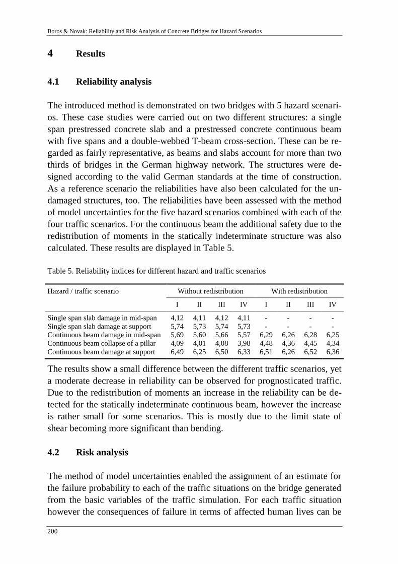
Boros & Novak: Reliability and Risk Analysis of Concrete Bridges for Hazard Scenarios
200
4 Results
4.1 Reliability analysis
The introduced method is demonstrated on two bridges with 5 hazard scenari-
os. These case studies were carried out on two different structures: a single
span prestressed concrete slab and a prestressed concrete continuous beam
with five spans and a double-webbed T-beam cross-section. These can be re-
garded as fairly representative, as beams and slabs account for more than two
thirds of bridges in the German highway network. The structures were de-
signed according to the valid German standards at the time of construction.
As a reference scenario the reliabilities have also been calculated for the un-
damaged structures, too. The reliabilities have been assessed with the method
of model uncertainties for the five hazard scenarios combined with each of the
four traffic scenarios. For the continuous beam the additional safety due to the
redistribution of moments in the statically indeterminate structure was also
calculated. These results are displayed in Table 5.
Table 5. Reliability indices for different hazard and traffic scenarios
Hazard / traffic scenario Without redistribution With redistribution
I II III IV I II III IV
Single span slab damage in mid-span
Single span slab damage at support
Continuous beam damage in mid-span
Continuous beam collapse of a pillar
Continuous beam damage at support
4,12
5,74
5,69
4,09
6,49
4,11
5,73
5,60
4,01
6,25
4,12
5,74
5,66
4,08
6,50
4,11
5,73
5,57
3,98
6,33
-
-
6,29
4,48
6,51
-
-
6,26
4,36
6,26
-
-
6,28
4,45
6,52
-
-
6,25
4,34
6,36
The results show a small difference between the different traffic scenarios, yet
a moderate decrease in reliability can be observed for prognosticated traffic.
Due to the redistribution of moments an increase in the reliability can be de-
tected for the statically indeterminate continuous beam, however the increase
is rather small for some scenarios. This is mostly due to the limit state of
shear becoming more significant than bending.
4.2 Risk analysis
The method of model uncertainties enabled the assignment of an estimate for
the failure probability to each of the traffic situations on the bridge generated
from the basic variables of the traffic simulation. For each traffic situation
however the consequences of failure in terms of affected human lives can be
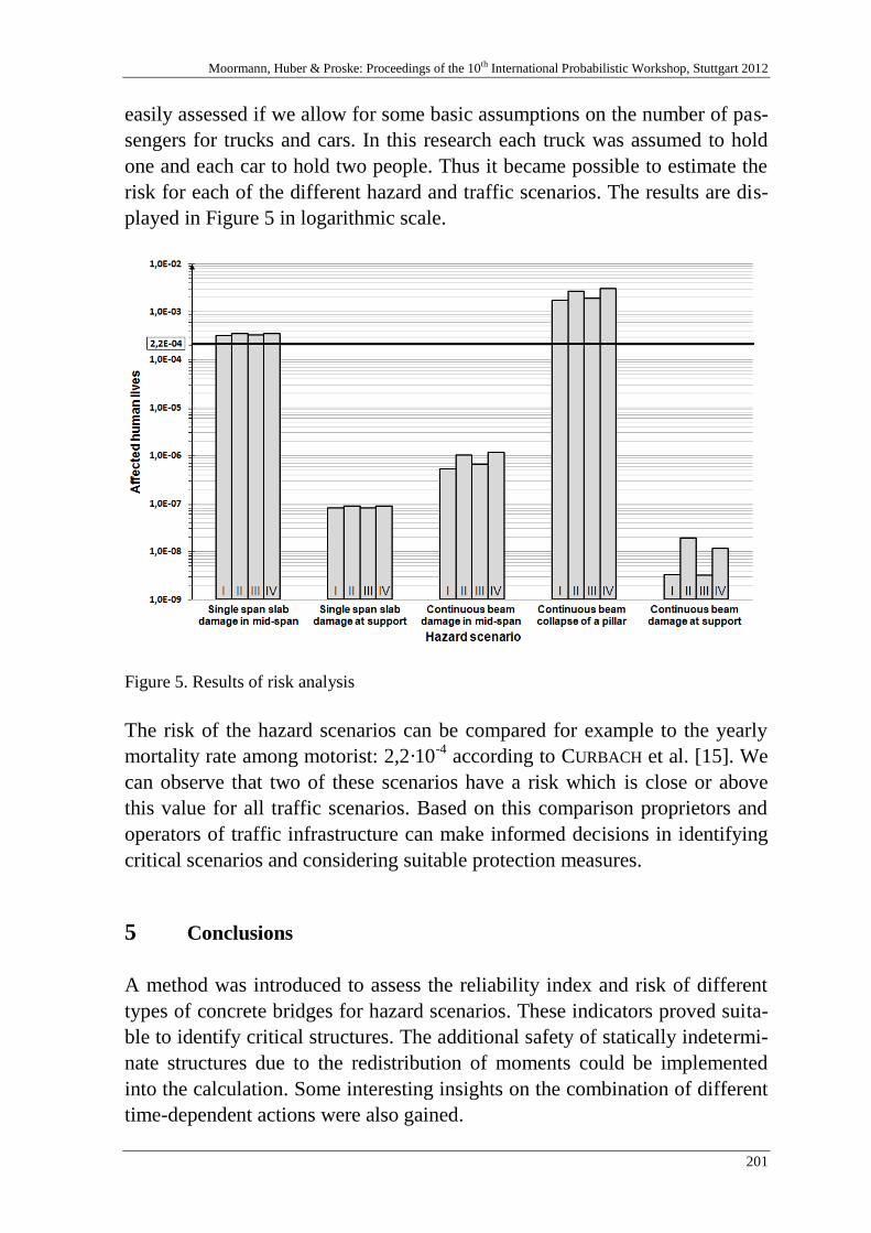
Moormann, Huber & Proske: Proceedings of the 10th International Probabilistic Workshop, Stuttgart 2012
201
easily assessed if we allow for some basic assumptions on the number of pas-
sengers for trucks and cars. In this research each truck was assumed to hold
one and each car to hold two people. Thus it became possible to estimate the
risk for each of the different hazard and traffic scenarios. The results are dis-
played in Figure 5 in logarithmic scale.
Figure 5. Results of risk analysis
The risk of the hazard scenarios can be compared for example to the yearly
mortality rate among motorist: 2,2·10-4
according to CURBACH et al. [15]. We
can observe that two of these scenarios have a risk which is close or above
this value for all traffic scenarios. Based on this comparison proprietors and
operators of traffic infrastructure can make informed decisions in identifying
critical scenarios and considering suitable protection measures.
5 Conclusions
A method was introduced to assess the reliability index and risk of different
types of concrete bridges for hazard scenarios. These indicators proved suita-
ble to identify critical structures. The additional safety of statically indetermi-
nate structures due to the redistribution of moments could be implemented
into the calculation. Some interesting insights on the combination of different
time-dependent actions were also gained.

Boros & Novak: Reliability and Risk Analysis of Concrete Bridges for Hazard Scenarios
202
6 Literature references
[1] SKRIBT Schlussbericht: Schutz kritischer Brücken und Tunnel im Zuge von Straßen,
Empfehlungen zur Maßnahmenanwendung für Brücken und Tunnel, in Vorbereitung
[2] Allgemeine bauaufsichtliche Zulassung Z-12.3-29, Spannstahllitzen St 1570/1770
aus 7 kaltgezogenen, glatten Einzeldrähten, Deutsches Institut für Bautechnik, 2004
[3] Six, M.: Sicherheitskonzept für nichtlineare Traglastverfahren im Betonbau, Deut-
scher Ausschuss für Stahlbeton Heft 534, 2003
[4] Joint Committee on Structural Safety, Probabilistic Model Code, 2001
[5] FE 89.0232/2009/AP Schlussbericht, Auswirkungen des Klimawandels auf beste-
hende Spannbetonbrückenbauwerke, 2011
[6] Frenzel, B. et al.: Bestimmung von Kombinationsbeiwerten und -regeln für Einwir-
kungen auf Brücken, Forschung Straßenbau und Straßenverkehrstechnik Heft 715,
Typo-Druck-& Verlaggesellschaft, Bonn, 1996
[7] Spaethe, G.: Die Sicherheit Tragender Baukonstruktionen, Springer, Wien, 1992
[8] Kaschner, R. et al., Auswirkungen des Schwerlastverkehrs auf die Brücken der Bun-
desfernstraßen, Berichte der Bundesanstalt für Straßenwesen Heft B 68, Verlag für
neue Wissenschaft, Bremerhaven, 2009
[9] FE 15.451/2007/FRB Schlussbericht, Anpassung des DIN-Fachberichtes „Einwir-
kungen auf Brücken“ an endgültige Eurocodes und nationale Anhänge einschließlich
Vergleichsrechnung, 2009
[10] Faber, M. H.: Risk and Safety in Engineering, ETH Zürich, 2009
[11] Rackwitz, R.: Zuverlässigkeit und Lasten im konstruktiven Ingenieurbau – Teil I:
Zuverlässigkeitstheoretische Grundlagen, Technische Universität München, 2006
[12] Boros, V.: Zur Zuverlässigkeitsanalyse von Massivbrücken für außergewöhnliche
Bedrohungsszenarien, Universität Stuttgart, 2012 - Dissertation
[13] Turkstra, C. J. et al.: Load Combinations in Codified Structural Design, Journal of
the Structural Division, Proceedings of the American Society of Civil Engineers 106
(1980), S. 2527-2543
[14] Ghosn, M. et al.: National Cooperative Highway Research Program Report 489,
Design of Highway Bridges for Extreme Events, Transportation Research Board,
Washington D. C., 2003
[15] Curbach M. et al.: Die Sicherheit von Brücken im Vergleich zu anderen Risiken, 12.
Dresdner Brückenbausymposium - Planung, Bauausführung und Ertüchtigung von
Massivbrücken, Dresden, 2002, S. 197

Moormann, Huber & Proske: Proceedings of the 10th International Probabilistic Workshop, Stuttgart 2012
203
Probabilistic Analysis Based on S-version
Finite Element Method of Surface Crack
Growth
MRM Akramin1, AK Ariffin
1, M Kikuchi
2, S Abdullah
1,
N Nikabdullah1, MS Shaari
1
1Faculty of Mechanical Engineering and Built Environment,
Universiti Kebangsaan Malaysia, Selangor, Malaysia.
2Tokyo University of Science, Yamazaki, Noda, Chiba, Japan.
Abstract: The complexity of 3D surface crack growth behavior is investigated
by the S-version Finite Element Method. The research work is focused on cy-
clic load, which gives an absolute picture of reality in an engineering world.
The Monte Carlo method is embedded with S-version Finite Element Method
for reliability analysis of the structural system with a mixture of random and
interval parameters and loadings. The purpose of employed the Monte-Carlo
method is to determine the reliability of the structure. Thus, mean values and
standard deviations of uncertain parameters need to be computed. The generat-
ed uncertain parameters by Monte-Carlo method are used for analysis in S-
version Finite Element Method. The S-version Finite Element Method is per-
formed by superposed the local dense finite element mesh on the global coarse
finite element mesh. An adaptive mesh refinement method is implemented,
which allows local refinement of the mesh without introducing a transition re-
gion. Based on S-version Finite Element Method results, probabilistic analysis
is conducted. Probabilistic analysis represents the uncertainty in modeling stud-
ies. It can offer the opportunity to view the impact of the uncertain parameters
statistically. Variabilities of material properties are presented in a probabilistic
analysis by using statistical distribution functions. The probability of failure
which is caused by uncertain loads and material properties in the structure is
estimated. Numerical example is presented to show that probabilistic analysis
based on S-version Finite Element Method simulation provides accurate esti-
mates of failure probability. The comparison shows that the combination be-
tween S-version Finite Element Method analysis and probabilistic analysis
provide a simple and realistic of quantify the failure probability.

Akramin, Ariffin, Kikuchi, Abdullah, Nikabdulla & Shaari: Probabilistic Analysis Based on S-version Finite Element
Method of Surface Crack Growth
204
1 Introduction
The existence of surface crack has been a major problem in pressurized thick-walled cylin-
ders and nuclear reactor structural. Surface crack as well frequently found in aeronautical
panel, cylinder of an extrusion press, riveted aeronautic reinforcement and pressure vessel.
The most happen to be in semielliptical form. Due to the complexity of the three-
dimensional surface crack, many researchers have used numerical approximation to obtain
the stress intensity factor. Thus, numerical calculation is one of the best remedy to solve
the complexity. Various methods have been developed such as Finite Element Method,
Extended-Finite Element Method and others. In this research work, S-version Finite Ele-
ment Method (s-FEM) was implemented for calculation of the stress intensity factor.
The s-FEM has been applied to diverse application ranges such as heat affected zone mate-
rial [1, 2], corrosion cracking [3], crack closure effect [4] and composite material [5]. Var-
ious types of load behavior [6-9] as well have been an issue in the numerical
implementation. The most striking one is the fatigue load since the fatigue load represented
a real case study in an engineering world. Fatigue load is a major fracture cause in a struc-
ture due to long term cyclic load. The integrity of the structure can be questioned when a
crack was discovered in a structure. Sustainability of the structure needs to evaluate in or-
der to avoid a fiasco, especially when a crack detected.
Therefore, in this study s-FEM is developed together with an analysis of residual fatigue
life. The prediction of fatigue crack growth rate is based on Paris law. The crack surface
introduced into the structure is considered. In s-FEM 3-dimensional simulation model,
fatigue load is applied throughout the process. Experimental works were carried out to val-
idate the simulation analysis data. The crack paths from simulation and experiment were
compared and discussed briefly. Afterward, the change of the stress intensity factors along
the cycle was investigated based on simulation results.
2 Methodology
The s-FEM was implemented in this study. Figure 1 shows the s-FEM concept. The coars-
er mesh was generated for global mesh while a denser mesh was used at near the crack tip
area. Crack tip area was taken into account during the implementation of local mesh. On
the global mesh, crack tip area was neglected temporarily.
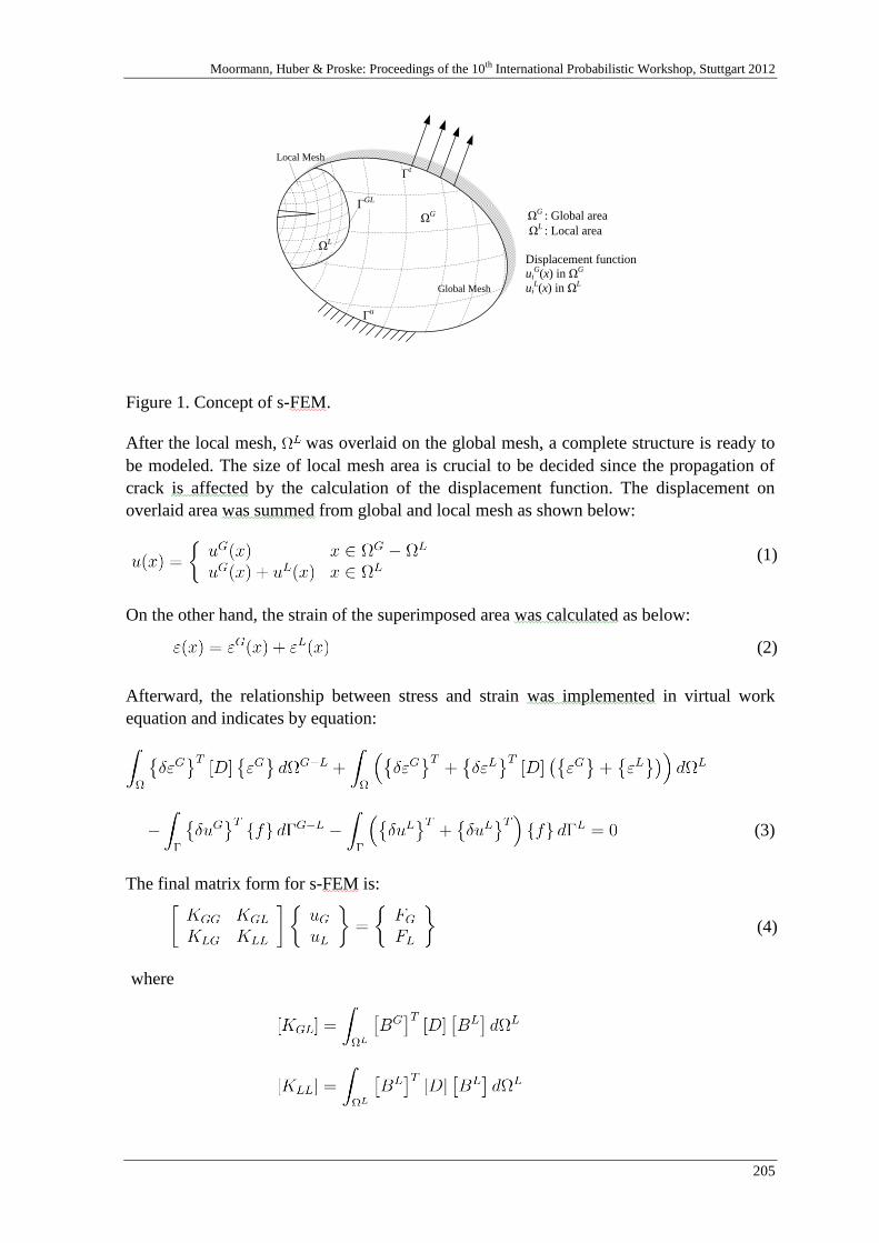
Moormann, Huber & Proske: Proceedings of the 10th International Probabilistic Workshop, Stuttgart 2012
205
Global Mesh
Local Mesh
ΩL
ΩG
Γt
Γu
ΓGL
ΩG : Global area
ΩL : Local area
Displacement function
uiG(x) in ΩG
uiL(x) in ΩL
Figure 1. Concept of s-FEM.
After the local mesh, was overlaid on the global mesh, a complete structure is ready to
be modeled. The size of local mesh area is crucial to be decided since the propagation of
crack is affected by the calculation of the displacement function. The displacement on
overlaid area was summed from global and local mesh as shown below:
(1)
On the other hand, the strain of the superimposed area was calculated as below:
(2)
Afterward, the relationship between stress and strain was implemented in virtual work
equation and indicates by equation:
(3)
The final matrix form for s-FEM is:
(4)
where
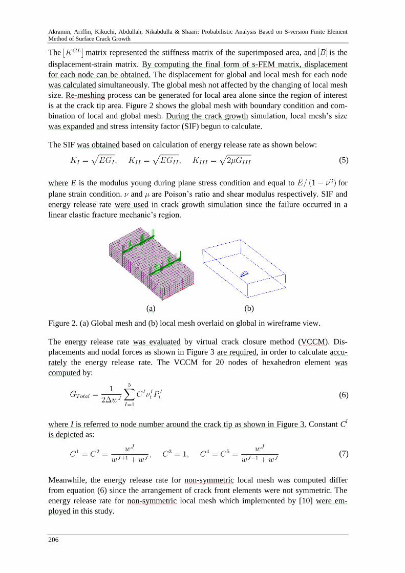
Akramin, Ariffin, Kikuchi, Abdullah, Nikabdulla & Shaari: Probabilistic Analysis Based on S-version Finite Element
Method of Surface Crack Growth
206
The matrix represented the stiffness matrix of the superimposed area, and is the
displacement-strain matrix. By computing the final form of s-FEM matrix, displacement
for each node can be obtained. The displacement for global and local mesh for each node
was calculated simultaneously. The global mesh not affected by the changing of local mesh
size. Re-meshing process can be generated for local area alone since the region of interest
is at the crack tip area. Figure 2 shows the global mesh with boundary condition and com-
bination of local and global mesh. During the crack growth simulation, local mesh’s size
was expanded and stress intensity factor (SIF) begun to calculate.
The SIF was obtained based on calculation of energy release rate as shown below:
(5)
where E is the modulus young during plane stress condition and equal to for
plane strain condition. and are Poison’s ratio and shear modulus respectively. SIF and
energy release rate were used in crack growth simulation since the failure occurred in a
linear elastic fracture mechanic’s region.
(a) (b)
Figure 2. (a) Global mesh and (b) local mesh overlaid on global in wireframe view.
The energy release rate was evaluated by virtual crack closure method (VCCM). Dis-
placements and nodal forces as shown in Figure 3 are required, in order to calculate accu-
rately the energy release rate. The VCCM for 20 nodes of hexahedron element was
computed by:
(6)
where I is referred to node number around the crack tip as shown in Figure 3. Constant CI
is depicted as:
(7)
Meanwhile, the energy release rate for non-symmetric local mesh was computed differ
from equation (6) since the arrangement of crack front elements were not symmetric. The
energy release rate for non-symmetric local mesh which implemented by [10] were em-
ployed in this study.
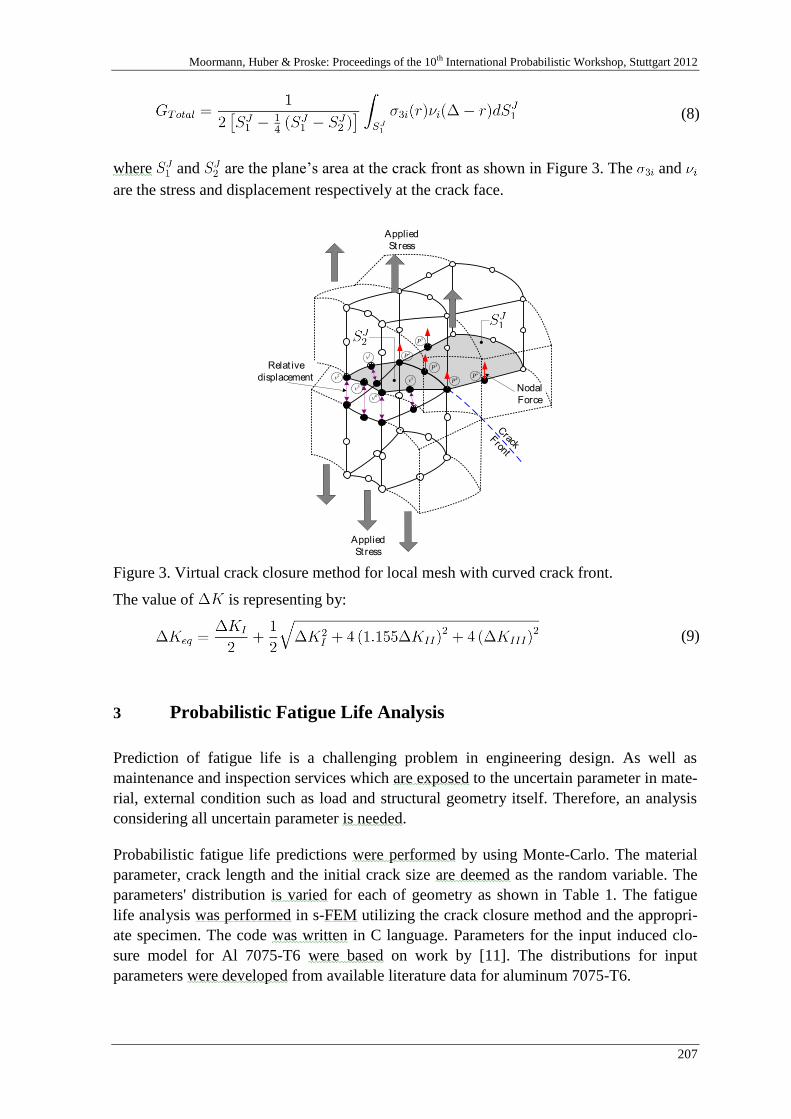
Moormann, Huber & Proske: Proceedings of the 10th International Probabilistic Workshop, Stuttgart 2012
207
(8)
where and are the plane’s area at the crack front as shown in Figure 3. The and
are the stress and displacement respectively at the crack face.
Crack
Front
Relat ive
displacementNodal
Force
Applied
St ress
Applied
St ress
ν1
ν5
ν4
ν3
ν2
P1
P2
P3
P4P5
Figure 3. Virtual crack closure method for local mesh with curved crack front.
The value of is representing by:
(9)
3 Probabilistic Fatigue Life Analysis
Prediction of fatigue life is a challenging problem in engineering design. As well as
maintenance and inspection services which are exposed to the uncertain parameter in mate-
rial, external condition such as load and structural geometry itself. Therefore, an analysis
considering all uncertain parameter is needed.
Probabilistic fatigue life predictions were performed by using Monte-Carlo. The material
parameter, crack length and the initial crack size are deemed as the random variable. The
parameters' distribution is varied for each of geometry as shown in Table 1. The fatigue
life analysis was performed in s-FEM utilizing the crack closure method and the appropri-
ate specimen. The code was written in C language. Parameters for the input induced clo-
sure model for Al 7075-T6 were based on work by [11]. The distributions for input
parameters were developed from available literature data for aluminum 7075-T6.

Akramin, Ariffin, Kikuchi, Abdullah, Nikabdulla & Shaari: Probabilistic Analysis Based on S-version Finite Element
Method of Surface Crack Growth
208
In probabilistic analysis, Paris coefficient, C of Al 7075-T6 was represented by mean
6.54x10⁻¹³
m/cycle with a standard deviation of 4.01x10⁻¹¹
m/cycle. The distribution was
assumed to be lognormal distribute based on the assumption made in the literature [11]. No
standard deviation for fatigue power parameter, n since it was set as deterministic. The
reason behind this was to control the acceleration of the crack growth in numerical calcula-
tion. Deterministic value of fatigue power parameter was computed since to monitor the
sensitivity of remaining distributed variable.
Young’s modulus was treated as a normal distribution as the variable changed accordingly
during the real application. Young’s modulus also has small coefficient of variation and
became the main reason for selecting Gaussian as the distribution.
4 Experiment
The surface crack was introduced by using four point bending test which conducted on the
0°, 15° and 45° specimens. Throughout the study, the aluminum alloy, A7075-T6 was cho-
sen as the material of the specimen. The specimens were imposed on two steps, which are
the initial step and after pre crack step. The differences between initial and after pre crack
steps are the protuberance and the dimension of the specimen after pre crack introduced.
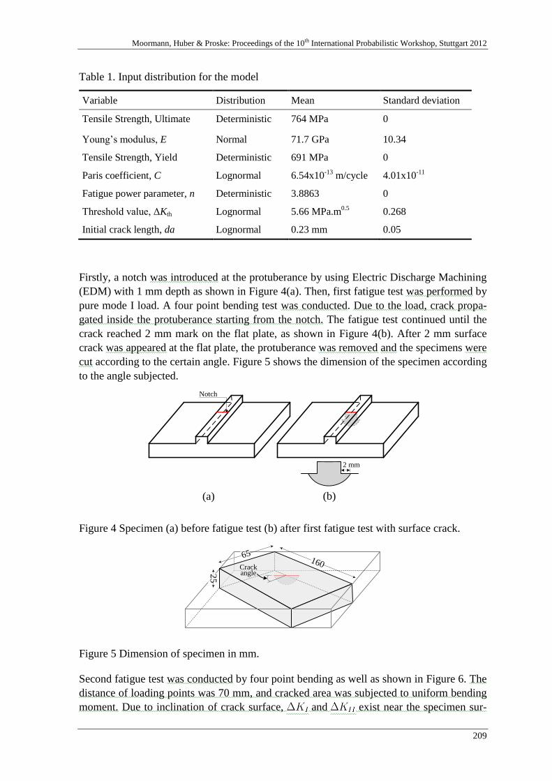
Moormann, Huber & Proske: Proceedings of the 10th International Probabilistic Workshop, Stuttgart 2012
209
Table 1. Input distribution for the model
Variable Distribution Mean Standard deviation
Tensile Strength, Ultimate Deterministic 764 MPa 0
Young’s modulus, E Normal 71.7 GPa 10.34
Tensile Strength, Yield Deterministic 691 MPa 0
Paris coefficient, C Lognormal 6.54x10⁻¹³
m/cycle 4.01x10⁻¹¹
Fatigue power parameter, n Deterministic 3.8863 0
Threshold value, ΔKth Lognormal 5.66 MPa.m0.5 0.268
Initial crack length, da Lognormal 0.23 mm 0.05
Firstly, a notch was introduced at the protuberance by using Electric Discharge Machining
(EDM) with 1 mm depth as shown in Figure 4(a). Then, first fatigue test was performed by
pure mode I load. A four point bending test was conducted. Due to the load, crack propa-
gated inside the protuberance starting from the notch. The fatigue test continued until the
crack reached 2 mm mark on the flat plate, as shown in Figure 4(b). After 2 mm surface
crack was appeared at the flat plate, the protuberance was removed and the specimens were
cut according to the certain angle. Figure 5 shows the dimension of the specimen according
to the angle subjected.
2 mm
Notch
(a) (b)
Figure 4 Specimen (a) before fatigue test (b) after first fatigue test with surface crack.
Crack angle
65160
25
Figure 5 Dimension of specimen in mm.
Second fatigue test was conducted by four point bending as well as shown in Figure 6. The
distance of loading points was 70 mm, and cracked area was subjected to uniform bending
moment. Due to inclination of crack surface, and exist near the specimen sur-

Akramin, Ariffin, Kikuchi, Abdullah, Nikabdulla & Shaari: Probabilistic Analysis Based on S-version Finite Element
Method of Surface Crack Growth
210
face. and exist at the deepest point of surface crack. Stress ratio 0.1 was used.
To measure the change of surface crack shape, beach mark was introduced by stress ratio
R=0.8.
140 mm
70 mm
Figure 6 Four point bending test.
5 Results and Discussion
The uncertain inputs data was generated according to its distribution with respect to mean
and standard deviation value as shown in Figure 7. The frequency of each random parame-
ter represented the distribution. Each parameter’s computations were compared with the
best fit cumulative distribution function. The parameters were shown that, it was generated
according to its distribution function.
The 95% confidence bounds of data inputs shown in Figure 8. All data inputs; Young’s
modulus, Paris coefficient, threshold value and initial crack length were generated within
the two standard deviation of each parameter. It showed the capability of developed s-FEM
code to generate random variables according to certain distribution.
In Figure 9, the simulation results for growth of the surface crack were compared with ex-
perimental results. The notch introduced at the early stage of the experimental process was
shown clearly in this figure as an initial for crack to growth. After the cyclic load was ap-
plied on the specimen, the pre-cracking was generated as shown in the plot. The pre-
cracking area was drawn in the graph. Crack growth for experimental works was started to
be observed after pre-cracking’s area. The same initial conditions introduced for numerical
model. As well as the size of pre-cracking area was modelled in local mesh. In this figure,
variations of crack growth shown as the results of the randomness of uncertain parameters.
It showed all possibilities that crack tend to growth with respect to certain random parame-
ters.
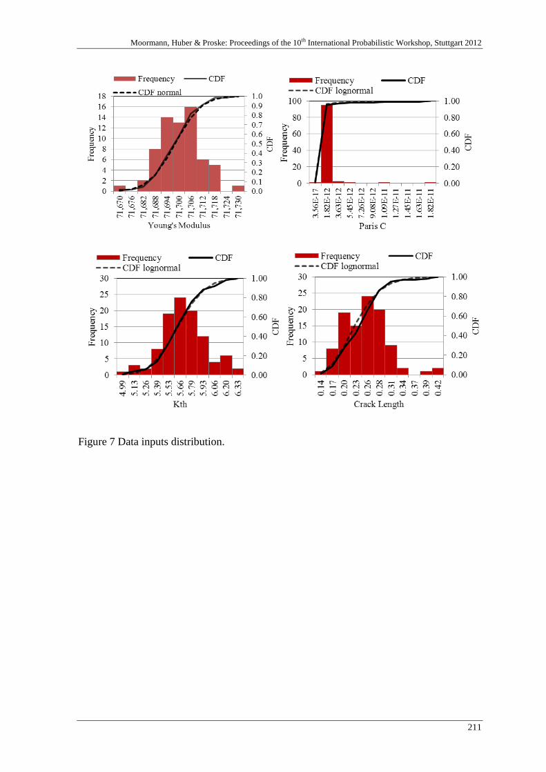
Moormann, Huber & Proske: Proceedings of the 10th International Probabilistic Workshop, Stuttgart 2012
211
Figure 7 Data inputs distribution.
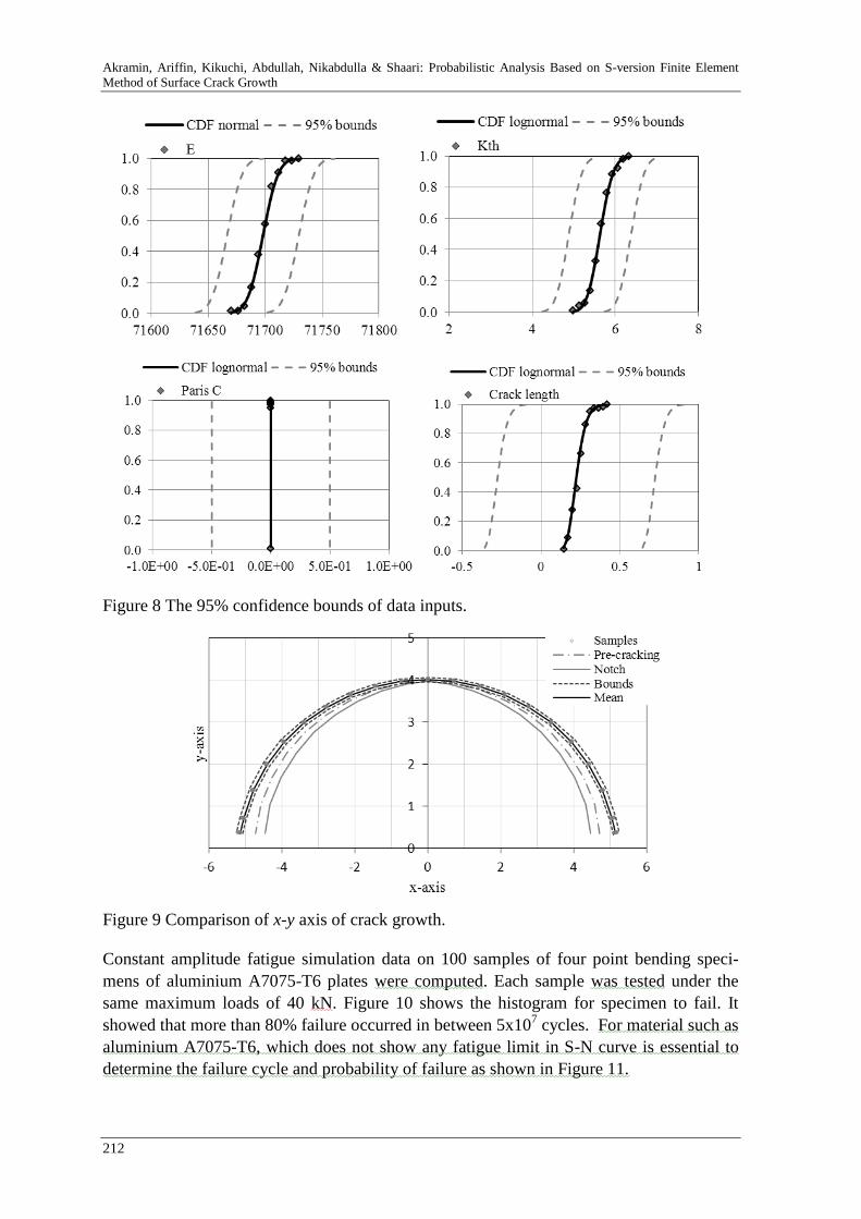
Akramin, Ariffin, Kikuchi, Abdullah, Nikabdulla & Shaari: Probabilistic Analysis Based on S-version Finite Element
Method of Surface Crack Growth
212
Figure 8 The 95% confidence bounds of data inputs.
Figure 9 Comparison of x-y axis of crack growth.
Constant amplitude fatigue simulation data on 100 samples of four point bending speci-
mens of aluminium A7075-T6 plates were computed. Each sample was tested under the
same maximum loads of 40 kN. Figure 10 shows the histogram for specimen to fail. It
showed that more than 80% failure occurred in between 5x10⁷ cycles. For material such as
aluminium A7075-T6, which does not show any fatigue limit in S-N curve is essential to
determine the failure cycle and probability of failure as shown in Figure 11.
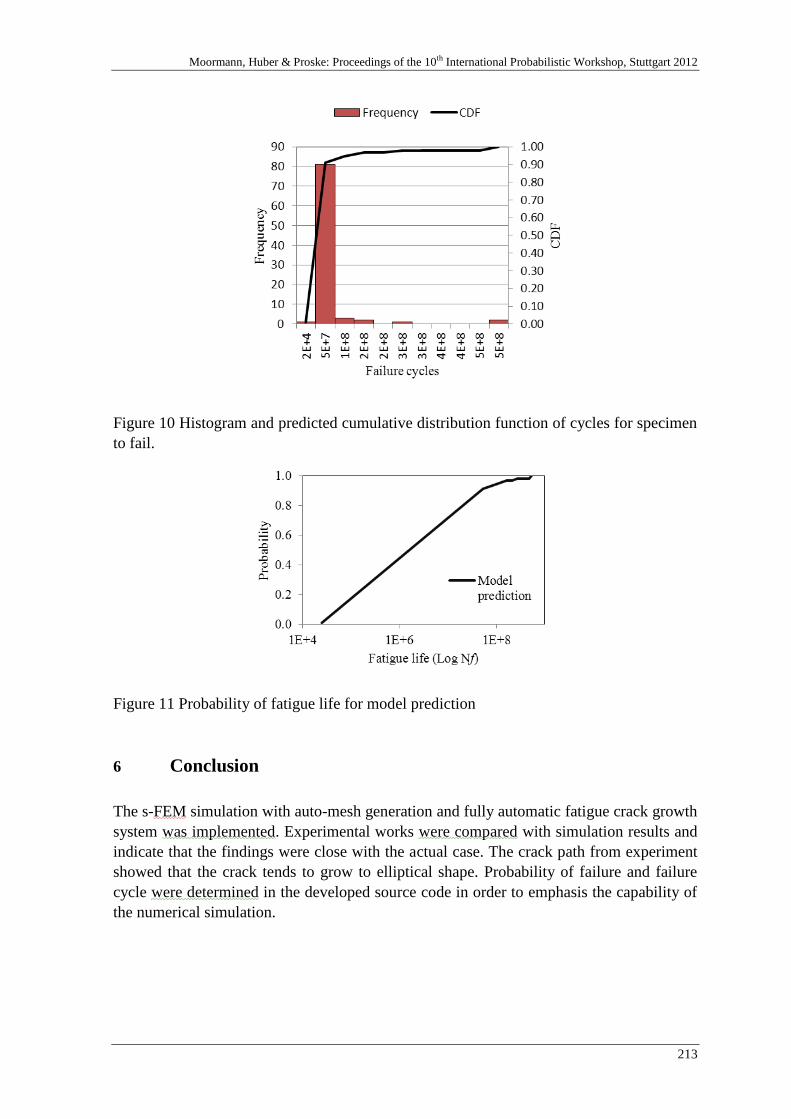
Moormann, Huber & Proske: Proceedings of the 10th International Probabilistic Workshop, Stuttgart 2012
213
Figure 10 Histogram and predicted cumulative distribution function of cycles for specimen
to fail.
Figure 11 Probability of fatigue life for model prediction
6 Conclusion
The s-FEM simulation with auto-mesh generation and fully automatic fatigue crack growth
system was implemented. Experimental works were compared with simulation results and
indicate that the findings were close with the actual case. The crack path from experiment
showed that the crack tends to grow to elliptical shape. Probability of failure and failure
cycle were determined in the developed source code in order to emphasis the capability of
the numerical simulation.

Akramin, Ariffin, Kikuchi, Abdullah, Nikabdulla & Shaari: Probabilistic Analysis Based on S-version Finite Element
Method of Surface Crack Growth
214
7 Reference
[1] Kikuchi, M.; Wada, Y.; Shimizu, Y.; Li, Y.: Crack growth analysis in a weld-heat-
affected zone using S-version FEM. International Journal of Pressure Vessels and
Piping, 90–910 (2012), P. 2-8.
[2] Kikuchi, M.; Wada, Y.; Shimizu, Y.; Yulong, L.: Crack growth analysis in weld-
heat affected zone using S-Version FEM. American Society of Mechanical
Engineers, Pressure Vessels and Piping Division. 2010 P. 401-406.
[3] Kikuchi, M.; Wada, Y.; Shmizu, Y.; Li, Y.: Stress corrosion cracking analysis
under thermal residual stress field using S-FEM. Key Engineering Materials 462-
463 (2011), P. 431-436.
[4] Kikuchi, M.; Wada, Y.; Maitireyimu, M.; Sano, H.: Closure effect on interaction of
two surface cracks under cyclic bending. American Society of Mechanical
Engineers, Pressure Vessels and Piping Division. 2010 P. 415-421.
[5] Angioni, S.L.; Visrolia, A.; Meo, M.: Combining X-FEM and a multilevel mesh
superposition method for the analysis of thick composite structures. Composites
Part B: Engineering, 432 (2012), P. 559-568.
[6] Kikuchi, M.; Wada, Y.; Suga, K.: Surface crack growth simulation under mixed
mode cyclic loading condition. Procedia Engineering. 2011 P. 427-432.
[7] Kikuchi, M.; Wada, Y.; Ohdama, C.: Effect of KIII on fatigue crack growth
behavior. American Society of Mechanical Engineers, Pressure Vessels and Piping
Division. 2010 P. 407-413.
[8] Kikuchi, M.; Wada, Y.; Suga, K.; Ohdama, C.: Effect of KIIIon fatigue crack
growth behavior (factory roof and fatigue crack growth rate). Nihon Kikai Gakkai
Ronbunshu, A Hen/Transactions of the Japan Society of Mechanical Engineers,
Part A, 76772 (2010), P. 1674-1680.
[9] Kikuchi, M.; Maitireymu, M.; Sano, H.: Study on fatigue crack growth criterion 1st
report, paris' law of a surface crack under pure mode i loading. Nihon Kikai Gakkai
Ronbunshu, A Hen/Transactions of the Japan Society of Mechanical Engineers,
Part A, 76764 (2010), P. 516-522.
[10] Okada, H.; Higashi, M.; Kikuchi, M.; Fukui, Y.; Kumazawa, N.: Three dimensional
virtual crack closure-integral method (VCCM) with skewed and non-symmetric
mesh arrangement at the crack front. Engineering Fracture Mechanics, 7211
(2005), P. 1717-1737.
[11] Liu, Y.; Mahadevan, S.: Probabilistic fatigue life prediction using an equivalent
initial flaw size distribution. International Journal of Fatigue, 313 (2009), P. 476-
487.

Moormann, Huber & Proske: Proceedings of the 10th International Probabilistic Workshop, Stuttgart 2012
215
Influence of soil heterogeneity on geotechnical
performance and uncertainty: a stochastic
view on EC7
Michael A. Hicks, Jonathan D. Nuttall
Section of Geo-Engineering, Faculty of Civil Engineering and Geosciences,
Delft University of Technology, Netherlands
Abstract: The spatial variability of soil properties affects soil behaviour and
geotechnical performance. It also leads to uncertainty in design due to incom-
plete knowledge about the ground conditions. This paper demonstrates how the
Random Finite Element Method (RFEM) may be used to quantify the perfor-
mance of geotechnical structures within a probabilistic framework, so account-
ing for the impact of heterogeneity on structure response, while, at the same
time, quantifying the uncertainty. In particular, it is shown that RFEM provides
a self-consistent framework for understanding the concept of characteristic
property values in Eurocode 7, as well as providing a means by which reliabil-
ity-based characteristic values may be determined. The procedure is demon-
strated for a 3D slope stability problem. Characteristic values are shown to be
problem dependent and a function of two competing factors: the spatial averag-
ing of properties along potential failure surfaces, which reduces the coefficient
of variation of the property values; and the tendency of failure mechanisms to
follow the path of least resistance, which causes an apparent reduction in the
property mean.
1 Introduction
Soils exhibit spatial variability of material properties. This spatial variability,
frequently referred to as heterogeneity, is anisotropic, often depth-dependent
and occurs at multiple scales: at the very small scale, as seen in the arrange-
ment of solid particles of sand or in the arrangement of fibres in fibrous mate-
rials such as peat; at the decimetre to metre scale, as observed in CPT
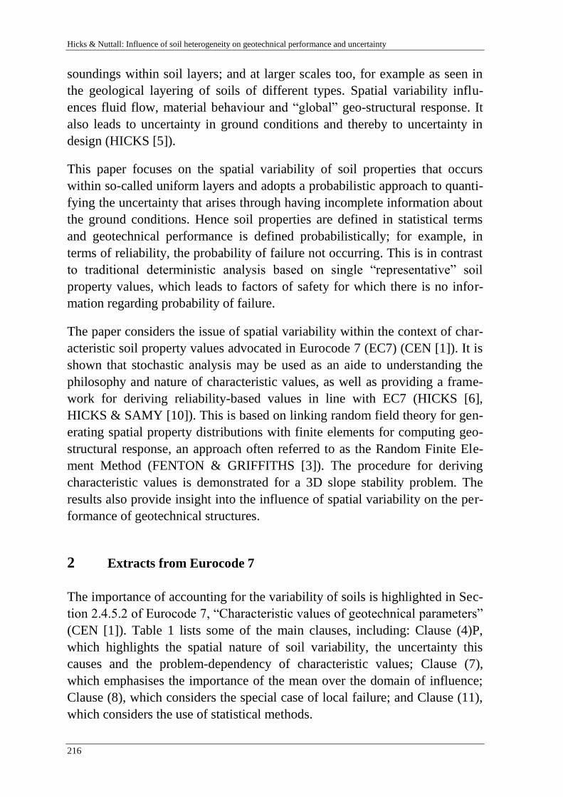
Hicks & Nuttall: Influence of soil heterogeneity on geotechnical performance and uncertainty
216
soundings within soil layers; and at larger scales too, for example as seen in
the geological layering of soils of different types. Spatial variability influ-
ences fluid flow, material behaviour and “global” geo-structural response. It
also leads to uncertainty in ground conditions and thereby to uncertainty in
design (HICKS [5]).
This paper focuses on the spatial variability of soil properties that occurs
within so-called uniform layers and adopts a probabilistic approach to quanti-
fying the uncertainty that arises through having incomplete information about
the ground conditions. Hence soil properties are defined in statistical terms
and geotechnical performance is defined probabilistically; for example, in
terms of reliability, the probability of failure not occurring. This is in contrast
to traditional deterministic analysis based on single “representative” soil
property values, which leads to factors of safety for which there is no infor-
mation regarding probability of failure.
The paper considers the issue of spatial variability within the context of char-
acteristic soil property values advocated in Eurocode 7 (EC7) (CEN [1]). It is
shown that stochastic analysis may be used as an aide to understanding the
philosophy and nature of characteristic values, as well as providing a frame-
work for deriving reliability-based values in line with EC7 (HICKS [6],
HICKS & SAMY [10]). This is based on linking random field theory for gen-
erating spatial property distributions with finite elements for computing geo-
structural response, an approach often referred to as the Random Finite Ele-
ment Method (FENTON & GRIFFITHS [3]). The procedure for deriving
characteristic values is demonstrated for a 3D slope stability problem. The
results also provide insight into the influence of spatial variability on the per-
formance of geotechnical structures.
2 Extracts from Eurocode 7
The importance of accounting for the variability of soils is highlighted in Sec-
tion 2.4.5.2 of Eurocode 7, “Characteristic values of geotechnical parameters”
(CEN [1]). Table 1 lists some of the main clauses, including: Clause (4)P,
which highlights the spatial nature of soil variability, the uncertainty this
causes and the problem-dependency of characteristic values; Clause (7),
which emphasises the importance of the mean over the domain of influence;
Clause (8), which considers the special case of local failure; and Clause (11),
which considers the use of statistical methods.

Moormann, Huber & Proske: Proceedings of the 10th International Probabilistic Workshop, Stuttgart 2012
217
Table 1. Extracts from Section 2.4.5.2 of Eurocode 7 (CEN [1])
No. Clause
(4)P
The selection of characteristic values for geotechnical parameters shall take account of
the following:
● geological and other background information, such as data from previous projects;
● the variability of measured property values and other relevant information, e.g. from
existing knowledge;
● the extent of the field and laboratory investigation;
● the type and number of samples;
● the extent of the zone of ground governing the behaviour of the geotechnical struc-
ture at the limit state being considered;
● the ability of the geotechnical structure to transfer loads from weak to strong zones
in the ground.
(7) The zone of ground governing the behaviour of a geotechnical structure at a limit state
is usually much larger than a test sample or the zone of ground affected in an in situ test.
Consequently the value of the governing parameter is often the mean of the range of
values covering a large surface or volume of the ground. The characteristic value should
be a cautious estimate of this mean value.
(8) If the behaviour of the geotechnical structure at the limit state considered is governed by
the lowest or highest value of the ground property, the characteristic value should be a
cautious estimate of the lowest or highest value occurring in the zone governing the
behaviour.
(11) If statistical methods are used, the characteristic value should be derived such that the
calculated probability of a worse value governing the occurrence of the limit state under
consideration is not greater than 5%.
NOTE: In this respect, a cautious estimate of the mean value is a selection of the mean
value of the limited set of geotechnical parameter values, with a confidence level of
95%; where local failure is concerned, a cautious estimate of the low value is a 5% frac-
tile.
HICKS [6] gave a detailed review of Section 2.4.5.2 by explaining selected
clauses, clarifying the relationship between clauses and addressing areas of
potential confusion. In particular, the paper focussed on the statistical defini-
tion of a characteristic value given in Clause (11) and explained how it is, de-
spite first appearances, completely consistent with Section 2.4.5.2 as a whole,
including Clauses (7) and (8) and the footnote to Clause (11). For this pur-
pose, HICKS [6] argued that the Random Finite Element Method provided a
self-consistent framework for quantifying and understanding the response of
geotechnical structures given soil heterogeneity, and for deriving characteris-
tic values satisfying the requirements of Eurocode 7 as demonstrated previ-
ously by HICKS & SAMY [10].
Clause (11) states that “the characteristic value should be derived such that
the calculated probability of a worse value governing the occurrence of the
limit state under consideration is not greater than 5%”. This implies a mini-
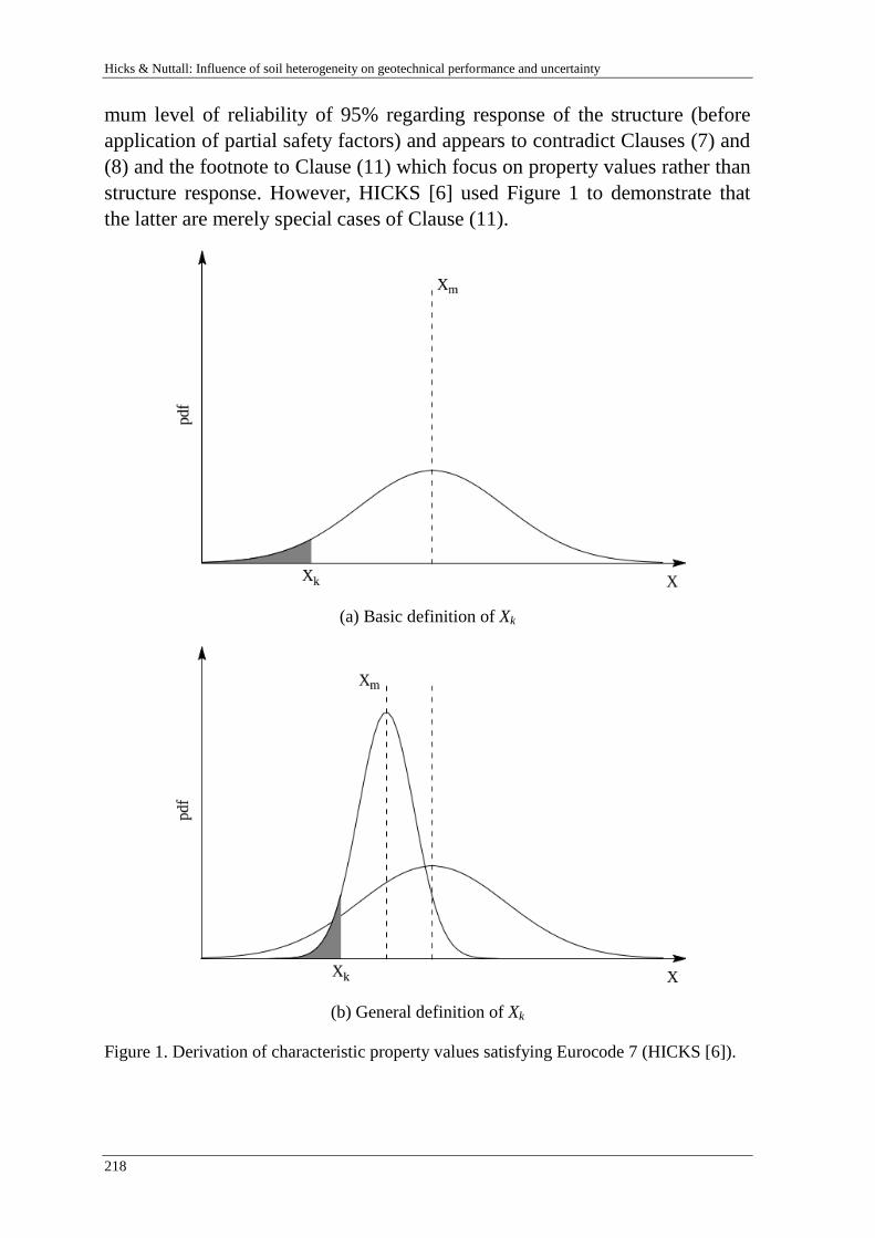
Hicks & Nuttall: Influence of soil heterogeneity on geotechnical performance and uncertainty
218
mum level of reliability of 95% regarding response of the structure (before
application of partial safety factors) and appears to contradict Clauses (7) and
(8) and the footnote to Clause (11) which focus on property values rather than
structure response. However, HICKS [6] used Figure 1 to demonstrate that
the latter are merely special cases of Clause (11).
(a) Basic definition of Xk
(b) General definition of Xk
Figure 1. Derivation of characteristic property values satisfying Eurocode 7 (HICKS [6]).
Moormann, Huber & Proske: Proceedings of the 10th International Probabilistic Workshop, Stuttgart 2012
219
2.1 Reliability-based characteristic values
Figure 1(a) shows the probability density function of a material property X,
which, to simplify the illustration, is assumed to be normal with a mean value
Xm. The simplest way to derive a reliability-based characteristic value Xk is to
proportion the area under the distribution as indicated. However, this is not
consistent with Clause (11) as it merely defines a value of Xk for which there
is a 95% probability of a larger value.
Figure 1(b) gives a more general derivation of Xk that is consistent with
Clause (11) and, by association, with all other clauses in Section 2.4.5.2. This
involves proportioning the area under a modified distribution of X that has
been back-figured from the response of the geotechnical structure itself. The
modified distribution is narrower than the underlying property distribution
due to the averaging of property values over potential failure surfaces. It is
also shifted to the left, due to the tendency for failure to propagate through
weaker zones. Hence, although it may be reasonable to take a conservative
estimate of the mean property value over a potential failure surface as the
characteristic value for that mechanism, this mean will generally be smaller
than the mean of the underlying property distribution. Variance reduction
methods may therefore give an unsafe solution if no account is taken of the
reduction in the mean.
HICKS [6] explained how the modified property distribution is a function of
the underlying distribution, the spatial correlation of property values, the
problem being analysed and the quality and extent of site investigation data.
Moreover, the modified distribution has two limits:
● When the spatial scale of fluctuation is very small relative to the problem
domain there is much averaging of soil properties, so that the standard de-
viation approaches zero and the mean tends to the mean of the underlying
distribution. In this case a cautious estimate of the mean is appropriate, as
advocated by Clause (7) and the first part of the footnote to Clause (11).
● When the spatial scale of fluctuation is very large relative to the problem
domain there is a very large range of possible solutions, so that the modi-
fied distribution approaches the underlying distribution. In this case Clause
(8) and the second part of the footnote to Clause (11) are relevant.
HICKS [6] also explained how the modified property distribution in Figure
1(b) may be derived for general problems. This is based on the work of
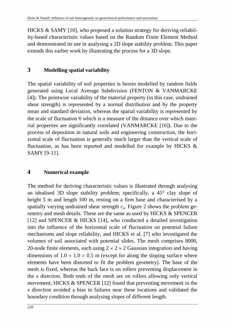
Hicks & Nuttall: Influence of soil heterogeneity on geotechnical performance and uncertainty
220
HICKS & SAMY [10], who proposed a solution strategy for deriving reliabil-
ity-based characteristic values based on the Random Finite Element Method
and demonstrated its use in analysing a 2D slope stability problem. This paper
extends this earlier work by illustrating the process for a 3D slope.
3 Modelling spatial variability
The spatial variability of soil properties is herein modelled by random fields
generated using Local Average Subdivision (FENTON & VANMARCKE
[4]). The pointwise variability of the material property (in this case, undrained
shear strength) is represented by a normal distribution and by the property
mean and standard deviation, whereas the spatial variability is represented by
the scale of fluctuation which is a measure of the distance over which mate-
rial properties are significantly correlated (VANMARCKE [16]). Due to the
process of deposition in natural soils and engineering construction, the hori-
zontal scale of fluctuation is generally much larger than the vertical scale of
fluctuation, as has been reported and modelled for example by HICKS &
SAMY [9-11].
4 Numerical example
The method for deriving characteristic values is illustrated through analysing
an idealised 3D slope stability problem; specifically, a 45° clay slope of
height 5 m and length 100 m, resting on a firm base and characterised by a
spatially varying undrained shear strength cu. Figure 2 shows the problem ge-
ometry and mesh details. These are the same as used by HICKS & SPENCER
[12] and SPENCER & HICKS [14], who conducted a detailed investigation
into the influence of the horizontal scale of fluctuation on potential failure
mechanisms and slope reliability, and HICKS et al. [7] who investigated the
volumes of soil associated with potential slides. The mesh comprises 8000,
20-node finite elements, each using 2 2 2 Gaussian integration and having
dimensions of 1.0 1.0 0.5 m (except for along the sloping surface where
elements have been distorted to fit the problem geometry). The base of the
mesh is fixed, whereas the back face is on rollers preventing displacement in
the x direction. Both ends of the mesh are on rollers allowing only vertical
movement; HICKS & SPENCER [12] found that preventing movement in the
x direction avoided a bias in failures near these locations and validated the
boundary condition through analysing slopes of different length.

Moormann, Huber & Proske: Proceedings of the 10th International Probabilistic Workshop, Stuttgart 2012
221
(a) Isometric projection
(b) Cross-section through mesh
Figure 2. Slope geometry and finite element mesh details (HICKS & SPENCER [12]).
In this investigation the clay is modelled by a linear elastic, perfectly plastic
soil model. The model’s elastic component is defined by a Young’s modulus,
E = 100000 kPa, and Poisson’s ratio, = 0.3, whereas the plastic component
comprises a Von Mises failure surface. The undrained shear strength is mod-
elled by a normal distribution with a mean of 40 kPa and a standard deviation
of 8 kPa. The vertical scale of fluctuation is v = 1.0 m, whereas a range of
possible values has been considered for the horizontal scale of fluctuation h.
4.1 Methodology
For each value of h a Monte Carlo simulation has been carried out, compris-
ing 250 realisations. Each realisation involves two steps: (a) the generation of
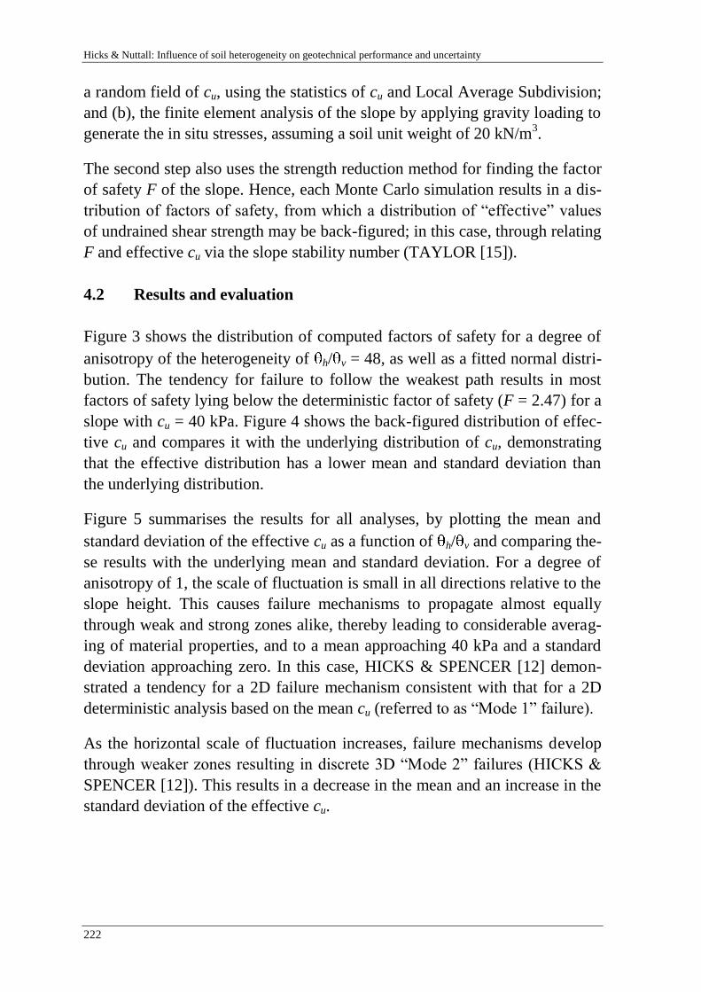
Hicks & Nuttall: Influence of soil heterogeneity on geotechnical performance and uncertainty
222
a random field of cu, using the statistics of cu and Local Average Subdivision;
and (b), the finite element analysis of the slope by applying gravity loading to
generate the in situ stresses, assuming a soil unit weight of 20 kN/m3.
The second step also uses the strength reduction method for finding the factor
of safety F of the slope. Hence, each Monte Carlo simulation results in a dis-
tribution of factors of safety, from which a distribution of “effective” values
of undrained shear strength may be back-figured; in this case, through relating
F and effective cu via the slope stability number (TAYLOR [15]).
4.2 Results and evaluation
Figure 3 shows the distribution of computed factors of safety for a degree of
anisotropy of the heterogeneity of h/ v = 48, as well as a fitted normal distri-
bution. The tendency for failure to follow the weakest path results in most
factors of safety lying below the deterministic factor of safety (F = 2.47) for a
slope with cu = 40 kPa. Figure 4 shows the back-figured distribution of effec-
tive cu and compares it with the underlying distribution of cu, demonstrating
that the effective distribution has a lower mean and standard deviation than
the underlying distribution.
Figure 5 summarises the results for all analyses, by plotting the mean and
standard deviation of the effective cu as a function of h/ v and comparing the-
se results with the underlying mean and standard deviation. For a degree of
anisotropy of 1, the scale of fluctuation is small in all directions relative to the
slope height. This causes failure mechanisms to propagate almost equally
through weak and strong zones alike, thereby leading to considerable averag-
ing of material properties, and to a mean approaching 40 kPa and a standard
deviation approaching zero. In this case, HICKS & SPENCER [12] demon-
strated a tendency for a 2D failure mechanism consistent with that for a 2D
deterministic analysis based on the mean cu (referred to as “Mode 1” failure).
As the horizontal scale of fluctuation increases, failure mechanisms develop
through weaker zones resulting in discrete 3D “Mode 2” failures (HICKS &
SPENCER [12]). This results in a decrease in the mean and an increase in the
standard deviation of the effective cu.
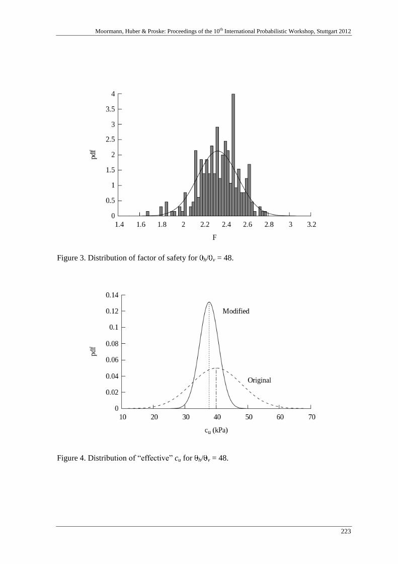
Moormann, Huber & Proske: Proceedings of the 10th International Probabilistic Workshop, Stuttgart 2012
223
Figure 3. Distribution of factor of safety for h/ v = 48.
Figure 4. Distribution of “effective” cu for h/ v = 48.
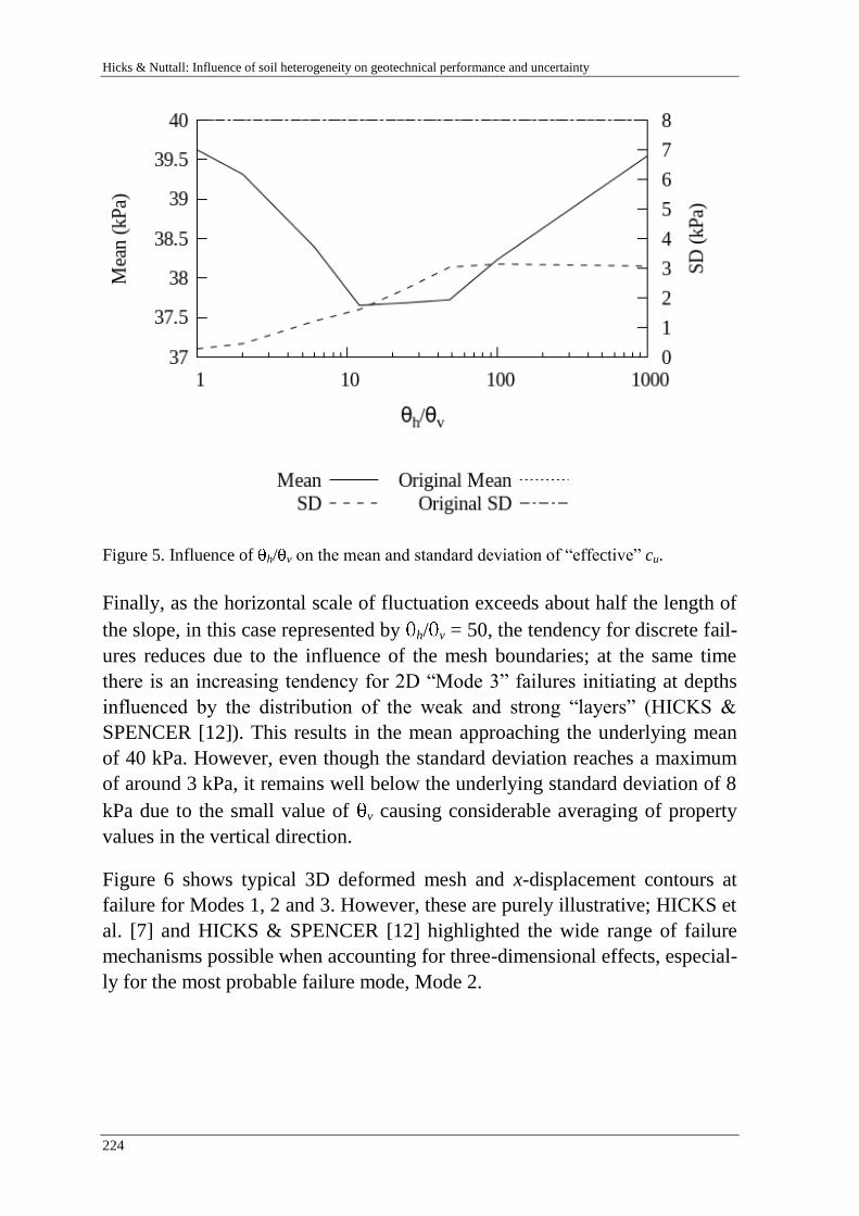
Hicks & Nuttall: Influence of soil heterogeneity on geotechnical performance and uncertainty
224
Figure 5. Influence of h/ v on the mean and standard deviation of “effective” cu.
Finally, as the horizontal scale of fluctuation exceeds about half the length of
the slope, in this case represented by h/ v = 50, the tendency for discrete fail-
ures reduces due to the influence of the mesh boundaries; at the same time
there is an increasing tendency for 2D “Mode 3” failures initiating at depths
influenced by the distribution of the weak and strong “layers” (HICKS &
SPENCER [12]). This results in the mean approaching the underlying mean
of 40 kPa. However, even though the standard deviation reaches a maximum
of around 3 kPa, it remains well below the underlying standard deviation of 8
kPa due to the small value of v causing considerable averaging of property
values in the vertical direction.
Figure 6 shows typical 3D deformed mesh and x-displacement contours at
failure for Modes 1, 2 and 3. However, these are purely illustrative; HICKS et
al. [7] and HICKS & SPENCER [12] highlighted the wide range of failure
mechanisms possible when accounting for three-dimensional effects, especial-
ly for the most probable failure mode, Mode 2.
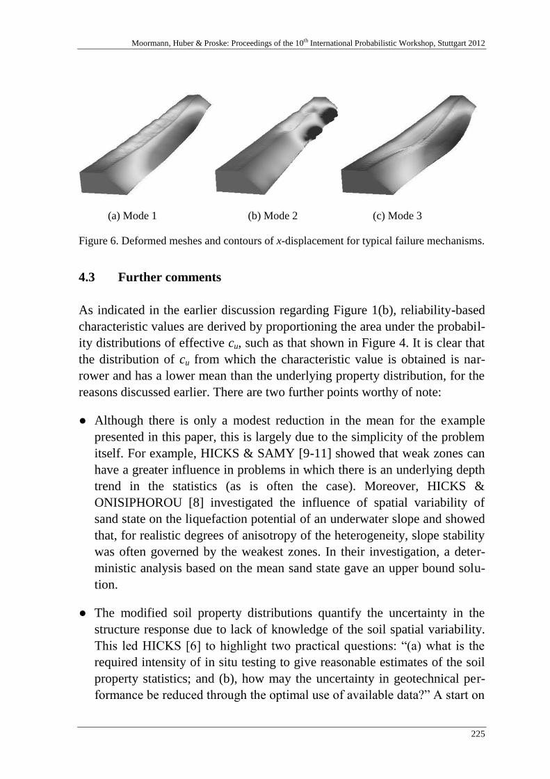
Moormann, Huber & Proske: Proceedings of the 10th International Probabilistic Workshop, Stuttgart 2012
225
(a) Mode 1 (b) Mode 2 (c) Mode 3
Figure 6. Deformed meshes and contours of x-displacement for typical failure mechanisms.
4.3 Further comments
As indicated in the earlier discussion regarding Figure 1(b), reliability-based
characteristic values are derived by proportioning the area under the probabil-
ity distributions of effective cu, such as that shown in Figure 4. It is clear that
the distribution of cu from which the characteristic value is obtained is nar-
rower and has a lower mean than the underlying property distribution, for the
reasons discussed earlier. There are two further points worthy of note:
● Although there is only a modest reduction in the mean for the example
presented in this paper, this is largely due to the simplicity of the problem
itself. For example, HICKS & SAMY [9-11] showed that weak zones can
have a greater influence in problems in which there is an underlying depth
trend in the statistics (as is often the case). Moreover, HICKS &
ONISIPHOROU [8] investigated the influence of spatial variability of
sand state on the liquefaction potential of an underwater slope and showed
that, for realistic degrees of anisotropy of the heterogeneity, slope stability
was often governed by the weakest zones. In their investigation, a deter-
ministic analysis based on the mean sand state gave an upper bound solu-
tion.
● The modified soil property distributions quantify the uncertainty in the
structure response due to lack of knowledge of the soil spatial variability.
This led HICKS [6] to highlight two practical questions: “(a) what is the
required intensity of in situ testing to give reasonable estimates of the soil
property statistics; and (b), how may the uncertainty in geotechnical per-
formance be reduced through the optimal use of available data?” A start on
Hicks & Nuttall: Influence of soil heterogeneity on geotechnical performance and uncertainty
226
addressing these issues has been made by VAN DEN EIJNDEN & HICKS
[2] and LLORET-CABOT et al. [13].
5 Conclusions
The influence of spatial variability of soil properties on geotechnical perfor-
mance and uncertainty has been demonstrated for an idealised 3D slope sta-
bility problem. As previously discussed by HICKS [6] and demonstrated by
HICKS & SAMY [10], the Random Finite Element Method may be used as a
basis for understanding and determining reliability-based characteristic values
in line with the requirements of Eurocode 7 (CEN [1]). HICKS [6] highlight-
ed that the modified property distribution, from which characteristic values
should be derived, is different to the underlying property distribution in two
respects: (a) it is narrower due to the averaging of properties over potential
failure surfaces; and (b), it has a reduced mean due to the tendency for failure
to follow the path of least resistance. This observation has been supported by
the results in this paper, reinforcing the view that variance reduction methods
may give an unsafe solution if no account is taken of the reduction in the
mean.
References
[1] CEN: Eurocode 7: Geotechnical design. Part 1: General rules, EN 1997-1. Europe-
an Committee for Standardisation (CEN), 2004.
[2] Eijnden, A.P. van den; Hicks, M.A.: Conditional simulation for characterizing the
spatial variability of sand state. In: Pietruszczak, S.; Pande, G.N. (Eds.): Proceedings
of the 2nd International Symposium on Computational Geomechanics. Dubrovnik,
Croatia, 2011, 288–296.
[3] Fenton, G.A.; Griffiths, D.V.: Risk assessment in geotechnical engineering. John
Wiley and Sons, 2008.
[4] Fenton, G.A.; Vanmarcke, E.H.: Simulation of random fields via Local Average
Subdivision, Journal of Engineering Mechanics, ASCE 116 (1990), 1733–1749.
[5] Hicks, M.A. (Ed.): Risk and variability in geotechnical engineering. Thomas Tel-
ford, London, 2007.
[6] Hicks, M.A.: An explanation of characteristic values of soil properties in Eurocode 7.
In: Arnold, P.; Fenton, G.A.; Hicks, M.A.; Schweckendiek, T.; Simpson, B. (Eds.):
Modern geotechnical design codes of practice: development, calibration and experi-
ences. IOS Press, 2012, in press.

Moormann, Huber & Proske: Proceedings of the 10th International Probabilistic Workshop, Stuttgart 2012
227
[7] Hicks, M.A.; Chen, J.; Spencer, W.A.: Influence of spatial variability on 3D slope
failures. In: Brebbia, C.A.; Beriatos, E. (Eds.): Proceedings of the 6th International
Conference on Computer Simulation Risk Analysis and Hazard Mitigation. Kefalo-
nia, Greece, 2008, 335–342.
[8] Hicks, M.A.; Onisiphorou, C.: Stochastic evaluation of static liquefaction in a pre-
dominantly dilative sand fill. Géotechnique 55 (2005), 123–133.
[9] Hicks, M.A.; Samy, K.: Influence of heterogeneity on undrained clay slope stability.
Quarterly Journal of Engineering Geology and Hydrogeology 35 (2002), 41–49.
[10] Hicks, M.A.; Samy, K.: Reliability-based characteristic values: a stochastic approach
to Eurocode 7. Ground Engineering 35 (2002), December, 30–34.
[11] Hicks, M.A.; Samy, K.: Stochastic evaluation of heterogeneous slope stability. Ital-
ian Geotechnical Engineering 38 (2004), 54–66.
[12] Hicks, M.A.; Spencer, W.A.: Influence of heterogeneity on the reliability and failure
of a long 3D slope. Computers and Geotechnics 37 (2010),
[13] Lloret-Cabot, M.; Hicks, M.A.; Eijnden, A.P. van den: Investigation of the reduction
in uncertainty due to soil variability when conditioning a random field using Kriging,
Géotechnique Letters 2 (2012), in press.
[14] Spencer, W.A.; Hicks, M.A.: A 3D finite element study of slope reliability. In: Pan-
de, G.N.; Pietruszczak, S. (Eds.): Proceedings of the 10th International Symposium
on Numerical Models in Geomechanics. Rhodes, Greece, 2007, 539–543.
[15] Taylor, D.W.: Stability of earth slopes. Journal of the Boston Society of Civil Engi-
neers 24 (1937), 197–246.
[16] Vanmarcke, E.H.: Random fields: Analysis and synthesis. The MIT Press, Cam-
bridge, Massachusetts, 1983.

Hicks & Nuttall: Influence of soil heterogeneity on geotechnical performance and uncertainty
228

Moormann, Huber & Proske: Proceedings of the 10th International Probabilistic Workshop, Stuttgart 2012
229
Uncertainty Analysis of stiffness prediction
for pile group models
Bastian Junga), Henning Stutz
a), Gudio Morgenthal
b), Frank Wuttke
c)
a) Research Training Group 1462,
b) Chair of Modelling and Simulation - Construction,
c) Chair of Geomechanical Modelling,
Bauhaus-Universität Weimar
Abstract: This paper presents a quantification of different vertical and lateral
pile group models. Therefore the chosen models are briefly introduced. The
uncertainty quantification for the total model uncertainty is then introduced.
This total model uncertainty is a combination of the model uncertainty and the
parameter uncertainty. After the introduction of the models and the uncertainty
analysis the investigated geometry and the stochastic input parameters are de-
scribed. The methodology is applied to the above-mentioned applications and
the results therefore are discussed.
1 Introduction
Model uncertainty is an important model property which has to be considered
for a reliable and therefore safe model application. DITHNDE et al. [3] stated,
that uncertainty analyses are essential especially in foundation engineering.
MOST [6] shows for the prediction and simulation of an appropriate structural
behaviour it is significant to consider a model choice evaluation including the
evaluation of the complexity and the prediction capability of the models. For
example, the research of SCHMOOR et al. [16] about the influence of the varia-
bility of soil and load parameters according a monopile does not take this
source of uncertainty into account. Taking this model prognosis uncertainty
into account can support the model selection process and can be the basis for
subsequent simulations like the above-mentioned reliability analyses [16].
Nowadays in bridge engineering, the use of integral or semi-integral struc-
tures is rising. This new development needs a holistic modelling of the com-
plete structure. One major part of these engineering structures is the
Jung, Stutz, Morgenthal & Wuttke: Uncertainty Analysis of stiffness prediction for pile group models
230
surrounding soil at the abutments and the pile-soil-pile interaction of the pier
foundations. Deflections and rotations of the foundation defined by their stiff-
ness prediction can reduce restraining forces in the structure in comparison to
the fixed foundation boundary conditions [11]. This paper focuses on differ-
ent models for the prediction of the vertical and lateral stiffness of pile group
foundations and their quantification of the total model uncertainty.
1.1 Vertical pile group models
Vertical loading on pile groups can be analysed using analytical solutions and
numerical techniques like the Finite Element Method or the Integral Equation
Analysis. A rather high number of different models for each methodology ex-
ist, which differ in their considered phenomenon for the piles, their interaction
in the group and the soil conditions. The research of RANDOLPH et al. about
the behaviour of single piles [13] and pile groups [14] is cited in almost every
publication afterwards and can be renowned as a fundamental approach to
determine the vertical stiffness of piles and piles groups. The interaction be-
tween the piles is dependent on the displacement field arising from the settle-
ment of a loaded (“source”) pile and therefore the piles follow the free-field
displacement generated by their neighbours, as an assumption (superposition
of individual pile displacement field). The model could be applied to any gen-
eral geometry of the pile group. The only restriction being that all the piles
must be embedded to the same depth. The soil behaviour is modelled as a lin-
ear-elastic material defined by the shear modulus which is assumed to vary
linearly with depth and a constant Poisson´s ratio.
MYLONAKIS et al. [7] used this model as their basis for further investigations.
The analytical formulation is based on the Winkler model of soil reaction for
determining the vertical interaction factors between two piles embedded in
multi-layered soil. In order to analyse this interaction, the interplay between
the adjacent (“receiver”) pile and the soil subjected to this displacement field
is additionally considered, in comparison to RANDOLPH et al. [14]. Axial pile
rigidity and the soil reaction at the pile tip tend to reduce the settlement based
on the assumption by [14].
In order to develop a practical design approach by determining nomogram,
RUDOLF [15] defined a numerical model for pile groups which take into ac-
count the partial safety concept. This model is developed based on extensive
parameter studies complemented by the results of extended analytical meth-
ods. The soil is modelled as a bi-linear material with a failure criteria defined
by Mohr-Coulomb.
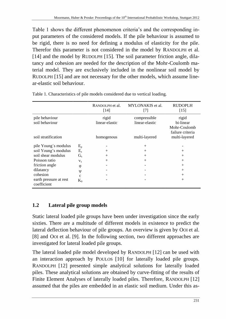
Moormann, Huber & Proske: Proceedings of the 10th International Probabilistic Workshop, Stuttgart 2012
231
Table 1 shows the different phenomenon criteria’s and the corresponding in-
put parameters of the considered models. If the pile behaviour is assumed to
be rigid, there is no need for defining a modulus of elasticity for the pile.
Therefor this parameter is not considered in the model by RANDOLPH et al.
[14] and the model by RUDOLPH [15]. The soil parameter friction angle, dila-
tancy and cohesion are needed for the description of the Mohr-Coulomb ma-
terial model. They are exclusively included in the nonlinear soil model by
RUDOLPH [15] and are not necessary for the other models, which assume line-
ar-elastic soil behaviour.
Table 1. Characteristics of pile models considered due to vertical loading.
RANDOLPH et al.
[14]
MYLONAKIS et al.
[7]
RUDOPLH
[15]
pile behaviour
soil behaviour
soil stratification
rigid
linear-elastic
homogenous
compressible
linear-elastic
multi-layered
rigid
bi-linear
Mohr-Coulomb
failure criteria
multi-layered
pile Young´s modulus
soil Young’s modulus
soil shear modulus
Poisson ratio
friction angle
dilatancy
cohesion
earth pressure at rest
coefficient
Ep
Es
Gs
s
c
K0
-
+
+
+
-
-
-
-
+
+
+
+
-
-
-
-
-
+
+
+
+
+
+
+
1.2 Lateral pile group models
Static lateral loaded pile groups have been under investigation since the early
sixties. There are a multitude of different models in existence to predict the
lateral deflection behaviour of pile groups. An overview is given by OOI et al.
[8] and OOI et al. [9]. In the following section, two different approaches are
investigated for lateral loaded pile groups.
The lateral loaded pile model developed by RANDOLPH [12] can be used with
an interaction approach by POULOS [10] for laterally loaded pile groups.
RANDOLPH [12] presented simple analytical solutions for laterally loaded
piles. These analytical solutions are obtained by curve-fitting of the results of
Finite Element Analyses of laterally loaded piles. Therefore, RANDOLPH [12]
assumed that the piles are embedded in an elastic soil medium. Under this as-
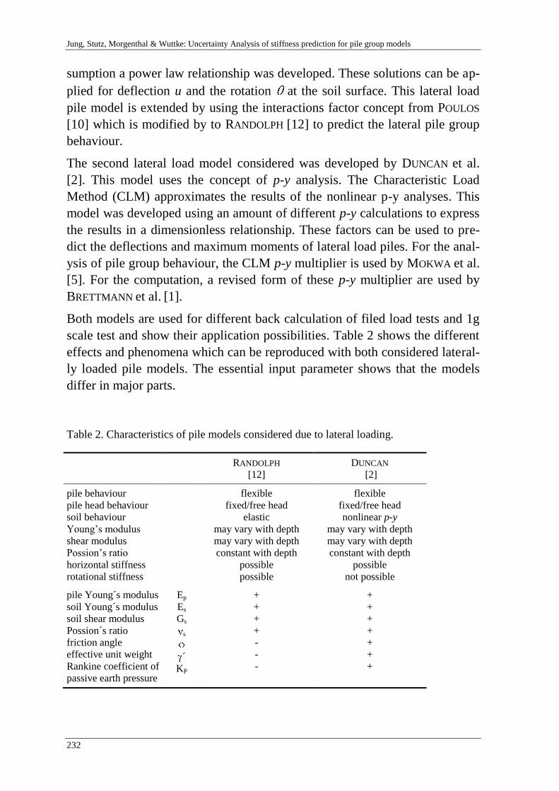
Jung, Stutz, Morgenthal & Wuttke: Uncertainty Analysis of stiffness prediction for pile group models
232
sumption a power law relationship was developed. These solutions can be ap-
plied for deflection u and the rotation at the soil surface. This lateral load
pile model is extended by using the interactions factor concept from POULOS
[10] which is modified by to RANDOLPH [12] to predict the lateral pile group
behaviour.
The second lateral load model considered was developed by DUNCAN et al.
[2]. This model uses the concept of p-y analysis. The Characteristic Load
Method (CLM) approximates the results of the nonlinear p-y analyses. This
model was developed using an amount of different p-y calculations to express
the results in a dimensionless relationship. These factors can be used to pre-
dict the deflections and maximum moments of lateral load piles. For the anal-
ysis of pile group behaviour, the CLM p-y multiplier is used by MOKWA et al.
[5]. For the computation, a revised form of these p-y multiplier are used by
BRETTMANN et al. [1].
Both models are used for different back calculation of filed load tests and 1g
scale test and show their application possibilities. Table 2 shows the different
effects and phenomena which can be reproduced with both considered lateral-
ly loaded pile models. The essential input parameter shows that the models
differ in major parts.
Table 2. Characteristics of pile models considered due to lateral loading.
RANDOLPH
[12]
DUNCAN
[2]
pile behaviour
pile head behaviour
soil behaviour
Young’s modulus
shear modulus
Possion’s ratio
horizontal stiffness
rotational stiffness
flexible
fixed/free head
elastic
may vary with depth
may vary with depth
constant with depth
possible
possible
flexible
fixed/free head
nonlinear p-y
may vary with depth
may vary with depth
constant with depth
possible
not possible
pile Young´s modulus
soil Young´s modulus
soil shear modulus
Possion´s ratio
friction angle
effective unit weight
Rankine coefficient of
passive earth pressure
Ep
Es
Gs
s
´
KP
+
+
+
+
-
-
-
+
+
+
+
+
+
+
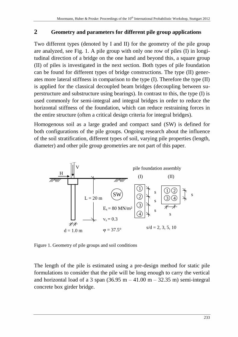
Moormann, Huber & Proske: Proceedings of the 10th International Probabilistic Workshop, Stuttgart 2012
233
2 Geometry and parameters for different pile group applications
Two different types (denoted by I and II) for the geometry of the pile group
are analyzed, see Fig. 1. A pile group with only one row of piles (I) in longi-
tudinal direction of a bridge on the one hand and beyond this, a square group
(II) of piles is investigated in the next section. Both types of pile foundation
can be found for different types of bridge constructions. The type (II) gener-
ates more lateral stiffness in comparison to the type (I). Therefore the type (II)
is applied for the classical decoupled beam bridges (decoupling between su-
perstructure and substructure using bearings). In contrast to this, the type (I) is
used commonly for semi-integral and integral bridges in order to reduce the
horizontal stiffness of the foundation, which can reduce restraining forces in
the entire structure (often a critical design criteria for integral bridges).
Homogenous soil as a large graded and compact sand (SW) is defined for
both configurations of the pile groups. Ongoing research about the influence
of the soil stratification, different types of soil, varying pile properties (length,
diameter) and other pile group geometries are not part of this paper.
Figure 1. Geometry of pile groups and soil conditions
The length of the pile is estimated using a pre-design method for static pile
formulations to consider that the pile will be long enough to carry the vertical
and horizontal load of a 3 span (36.95 m – 41.00 m – 32.35 m) semi-integral
concrete box girder bridge.
V pile foundation assembly
L = 20 m
Es = 80 MN/m²
s = 0.3
= 37.5°
SW 1
2
3
4
s/d = 2, 3, 5, 10
s
1 2
3 4
s
s
d = 1.0 m
s
s
(I) (II) H
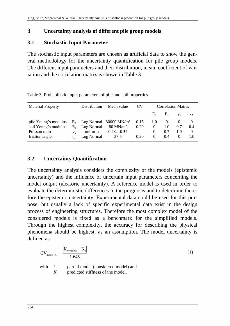
Jung, Stutz, Morgenthal & Wuttke: Uncertainty Analysis of stiffness prediction for pile group models
234
3 Uncertainty analysis of different pile group models
3.1 Stochastic Input Parameter
The stochastic input parameters are chosen as artificial data to show the gen-
eral methodology for the uncertainty quantification for pile group models.
The different input parameters and their distribution, mean, coefficient of var-
iation and the correlation matrix is shown in Table 3.
Table 3. Probabilistic input parameters of pile and soil properties.
Material Property Distribution
Mean value
CV
Correlation Matrix
Ep Es s
pile Young´s modulus
soil Young’s modulus
Poisson ratio
friction angle
Ep
Es
s
Log Normal
Log Normal
uniform
Log Normal
30000 MN/m²
80 MN/m²
0.28…0.32
37.5
0.15
0.20
-
0.20
1.0
0
0
0
0
1.0
0.7
0.4
0
0.7
1.0
0
0
0.4
0
1.0
3.2 Uncertainty Quantification
The uncertainty analysis considers the complexity of the models (epistemic
uncertainty) and the influence of uncertain input parameters concerning the
model output (aleatoric uncertainty). A reference model is used in order to
evaluate the deterministic differences in the prognosis and to determine there-
fore the epistemic uncertainty. Experimental data could be used for this pur-
pose, but usually a lack of specific experimental data exist in the design
process of engineering structures. Therefore the most complex model of the
considered models is fixed as a benchmark for the simplified models.
Through the highest complexity, the accuracy for describing the physical
phenomena should be highest, as an assumption. The model uncertainty is
defined as:
645.1
KKCV
icomplex
K,elmod i (1)
with i partial model (considered model) and
K predicted stiffness of the model.
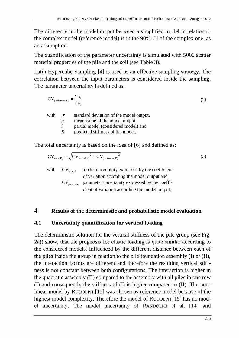
Moormann, Huber & Proske: Proceedings of the 10th International Probabilistic Workshop, Stuttgart 2012
235
The difference in the model output between a simplified model in relation to
the complex model (reference model) is in the 90%-CI of the complex one, as
an assumption.
The quantification of the parameter uncertainty is simulated with 5000 scatter
material properties of the pile and the soil (see Table 3).
Latin Hypercube Sampling [4] is used as an effective sampling strategy. The
correlation between the input parameters is considered inside the sampling.
The parameter uncertainty is defined as:
i
i
i
K
K
K,parameterCV (2)
with standard deviation of the model output,
µ mean value of the model output,
i partial model (considered model) and
K predicted stiffness of the model.
The total uncertainty is based on the idea of [6] and defined as:
2
K,parameter
2
K,elmodK,total iiiCVCVCV (3)
with elmodCV model uncertainty expressed by the coefficient
of variation according the model output and
paramaterCV parameter uncertainty expressed by the coeffi-
cient of variation according the model output.
4 Results of the deterministic and probabilistic model evaluation
4.1 Uncertainty quantification for vertical loading
The deterministic solution for the vertical stiffness of the pile group (see Fig.
2a)) show, that the prognosis for elastic loading is quite similar according to
the considered models. Influenced by the different distance between each of
the piles inside the group in relation to the pile foundation assembly (I) or (II),
the interaction factors are different and therefore the resulting vertical stiff-
ness is not constant between both configurations. The interaction is higher in
the quadratic assembly (II) compared to the assembly with all piles in one row
(I) and consequently the stiffness of (I) is higher compared to (II). The non-
linear model by RUDOLPH [15] was chosen as reference model because of the
highest model complexity. Therefore the model of RUDOLPH [15] has no mod-
el uncertainty. The model uncertainty of RANDOLPH et al. [14] and
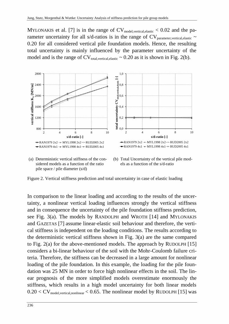
Jung, Stutz, Morgenthal & Wuttke: Uncertainty Analysis of stiffness prediction for pile group models
236
MYLONAKIS et al. [7] is in the range of CVmodel,vertical,elastic < 0.02 and the pa-
rameter uncertainty for all s/d-ratios is in the range of CVparameter,vertical,elastic ~
0.20 for all considered vertical pile foundation models. Hence, the resulting
total uncertainty is mainly influenced by the parameter uncertainty of the
model and is the range of CVtotal,vertical,elastic ~ 0.20 as it is shown in Fig. 2(b).
800
1200
1600
2000
2400
2800
2 4 6 8 10
ver
tica
l st
iffn
ess
KV
[MN
/m]
s/d-ratio [-]
RAN1979 2x2 MYL1998 2x2 RUD2005 2x2
RAN1979 4x1 MYL1998 4x1 RUD2005 4x1
0,0
0,2
0,4
0,6
0,8
1,0
2 4 6 8 10
tota
l u
nce
rta
inty
CV
tota
l,v
erti
cal,
ela
stic
[-]
s/d-ratio [-]
RAN1979 2x2 MYL1998 2x2 RUD2005 2x2
RAN1979 4x1 MYL1998 4x1 RUD2005 4x1
(a) Deterministic vertical stiffness of the con-
sidered models as a function of the ratio
pile space / pile diameter (s/d)
(b) Total Uncertainty of the vertical pile mod-
els as a function of the s/d-ratio
Figure 2. Vertical stiffness prediction and total uncertainty in case of elastic loading
In comparison to the linear loading and according to the results of the uncer-
tainty, a nonlinear vertical loading influences strongly the vertical stiffness
and in consequence the uncertainty of the pile foundation stiffness prediction,
see Fig. 3(a). The models by RANDOLPH and WROTH [14] and MYLONAKIS
and GAZETAS [7] assume linear-elastic soil behaviour and therefore, the verti-
cal stiffness is independent on the loading conditions. The results according to
the deterministic vertical stiffness shown in Fig. 3(a) are the same compared
to Fig. 2(a) for the above-mentioned models. The approach by RUDOLPH [15]
considers a bi-linear behaviour of the soil with the Mohr-Coulomb failure cri-
teria. Therefore, the stiffness can be decreased in a large amount for nonlinear
loading of the pile foundation. In this example, the loading for the pile foun-
dation was 25 MN in order to force high nonlinear effects in the soil. The lin-
ear prognosis of the more simplified models overestimate enormously the
stiffness, which results in a high model uncertainty for both linear models
0.20 < CVmodel,vertical,nonlinear < 0.65. The nonlinear model by RUDOLPH [15] was
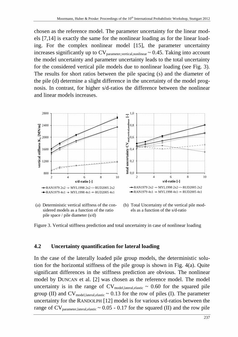
Moormann, Huber & Proske: Proceedings of the 10th International Probabilistic Workshop, Stuttgart 2012
237
chosen as the reference model. The parameter uncertainty for the linear mod-
els [7,14] is exactly the same for the nonlinear loading as for the linear load-
ing. For the complex nonlinear model [15], the parameter uncertainty
increases significantly up to CVparameter,vertical,nonlinear ~ 0.45. Taking into account
the model uncertainty and parameter uncertainty leads to the total uncertainty
for the considered vertical pile models due to nonlinear loading (see Fig. 3).
The results for short ratios between the pile spacing (s) and the diameter of
the pile (d) determine a slight difference in the uncertainty of the model prog-
nosis. In contrast, for higher s/d-ratios the difference between the nonlinear
and linear models increases.
800
1200
1600
2000
2400
2800
2 4 6 8 10
ver
tica
l st
iffn
ess
KV
[MN
/m]
s/d-ratio [-]
RAN1979 2x2 MYL1998 2x2 RUD2005 2x2
RAN1979 4x1 MYL1998 4x1 RUD2005 4x1
0,0
0,2
0,4
0,6
0,8
1,0
2 4 6 8 10
tota
l u
nce
rta
inty
CV
tota
l,ver
tica
l,n
on
lin
ear
[-]
s/d-ratio [-]
RAN1979 2x2 MYL1998 2x2 RUD2005 2x2
RAN1979 4x1 MYL1998 4x1 RUD2005 4x1
(a) Deterministic vertical stiffness of the con-
sidered models as a function of the ratio
pile space / pile diameter (s/d)
(b) Total Uncertainty of the vertical pile mod-
els as a function of the s/d-ratio
Figure 3. Vertical stiffness prediction and total uncertainty in case of nonlinear loading
4.2 Uncertainty quantification for lateral loading
In the case of the laterally loaded pile group models, the deterministic solu-
tion for the horizontal stiffness of the pile group is shown in Fig. 4(a). Quite
significant differences in the stiffness prediction are obvious. The nonlinear
model by DUNCAN et al. [2] was chosen as the reference model. The model
uncertainty is in the range of CVmodel,lateral,elastic ~ 0.60 for the squared pile
group (II) and CVmodel,lateral,elastic ~ 0.13 for the row of piles (I). The parameter
uncertainty for the RANDOLPH [12] model is for various s/d-ratios between the
range of CVparameter,lateral,elastic ~ 0.05 - 0.17 for the squared (II) and the row pile
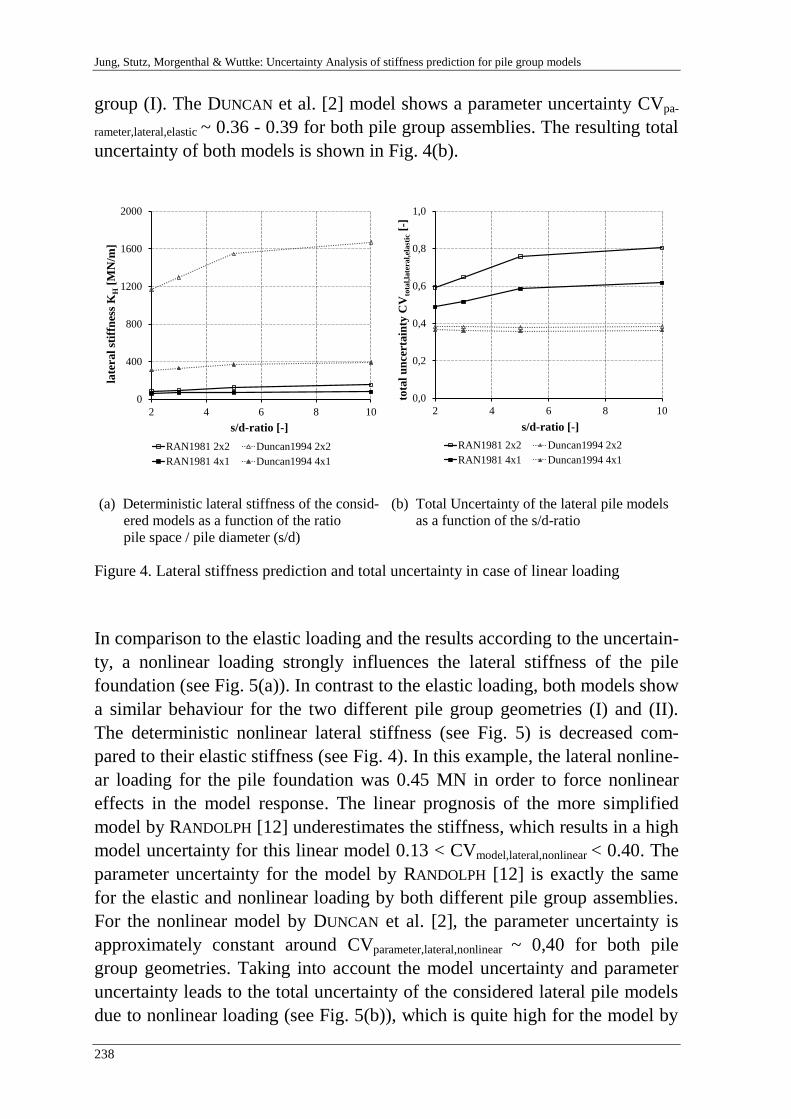
Jung, Stutz, Morgenthal & Wuttke: Uncertainty Analysis of stiffness prediction for pile group models
238
group (I). The DUNCAN et al. [2] model shows a parameter uncertainty CVpa-
rameter,lateral,elastic ~ 0.36 - 0.39 for both pile group assemblies. The resulting total
uncertainty of both models is shown in Fig. 4(b).
0
400
800
1200
1600
2000
2 4 6 8 10
late
ral
stif
fnes
s K
H[M
N/m
]
s/d-ratio [-]
RAN1981 2x2 Duncan1994 2x2
RAN1981 4x1 Duncan1994 4x1
0,0
0,2
0,4
0,6
0,8
1,0
2 4 6 8 10to
tal
un
cert
ain
ty C
Vto
tal,
late
ral,
ela
stic
[-]
s/d-ratio [-]
RAN1981 2x2 Duncan1994 2x2
RAN1981 4x1 Duncan1994 4x1
(a) Deterministic lateral stiffness of the consid-
ered models as a function of the ratio
pile space / pile diameter (s/d)
(b) Total Uncertainty of the lateral pile models
as a function of the s/d-ratio
Figure 4. Lateral stiffness prediction and total uncertainty in case of linear loading
In comparison to the elastic loading and the results according to the uncertain-
ty, a nonlinear loading strongly influences the lateral stiffness of the pile
foundation (see Fig. 5(a)). In contrast to the elastic loading, both models show
a similar behaviour for the two different pile group geometries (I) and (II).
The deterministic nonlinear lateral stiffness (see Fig. 5) is decreased com-
pared to their elastic stiffness (see Fig. 4). In this example, the lateral nonline-
ar loading for the pile foundation was 0.45 MN in order to force nonlinear
effects in the model response. The linear prognosis of the more simplified
model by RANDOLPH [12] underestimates the stiffness, which results in a high
model uncertainty for this linear model 0.13 < CVmodel,lateral,nonlinear < 0.40. The
parameter uncertainty for the model by RANDOLPH [12] is exactly the same
for the elastic and nonlinear loading by both different pile group assemblies.
For the nonlinear model by DUNCAN et al. [2], the parameter uncertainty is
approximately constant around CVparameter,lateral,nonlinear ~ 0,40 for both pile
group geometries. Taking into account the model uncertainty and parameter
uncertainty leads to the total uncertainty of the considered lateral pile models
due to nonlinear loading (see Fig. 5(b)), which is quite high for the model by
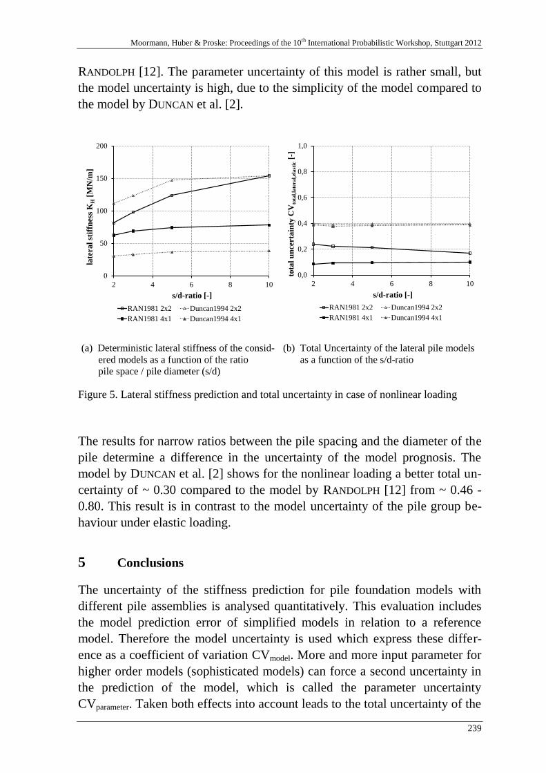
Moormann, Huber & Proske: Proceedings of the 10th International Probabilistic Workshop, Stuttgart 2012
239
RANDOLPH [12]. The parameter uncertainty of this model is rather small, but
the model uncertainty is high, due to the simplicity of the model compared to
the model by DUNCAN et al. [2].
0
50
100
150
200
2 4 6 8 10
late
ral
stif
fness
KH
[MN
/m]
s/d-ratio [-]
RAN1981 2x2 Duncan1994 2x2
RAN1981 4x1 Duncan1994 4x1
0,0
0,2
0,4
0,6
0,8
1,0
2 4 6 8 10to
tal
un
cert
ain
ty C
Vto
tal,
late
ral,
ela
stic
[-]
s/d-ratio [-]
RAN1981 2x2 Duncan1994 2x2
RAN1981 4x1 Duncan1994 4x1
(a) Deterministic lateral stiffness of the consid-
ered models as a function of the ratio
pile space / pile diameter (s/d)
(b) Total Uncertainty of the lateral pile models
as a function of the s/d-ratio
Figure 5. Lateral stiffness prediction and total uncertainty in case of nonlinear loading
The results for narrow ratios between the pile spacing and the diameter of the
pile determine a difference in the uncertainty of the model prognosis. The
model by DUNCAN et al. [2] shows for the nonlinear loading a better total un-
certainty of ~ 0.30 compared to the model by RANDOLPH [12] from ~ 0.46 -
0.80. This result is in contrast to the model uncertainty of the pile group be-
haviour under elastic loading.
5 Conclusions
The uncertainty of the stiffness prediction for pile foundation models with
different pile assemblies is analysed quantitatively. This evaluation includes
the model prediction error of simplified models in relation to a reference
model. Therefore the model uncertainty is used which express these differ-
ence as a coefficient of variation CVmodel. More and more input parameter for
higher order models (sophisticated models) can force a second uncertainty in
the prediction of the model, which is called the parameter uncertainty
CVparameter. Taken both effects into account leads to the total uncertainty of the
Jung, Stutz, Morgenthal & Wuttke: Uncertainty Analysis of stiffness prediction for pile group models
240
considered models CVtotal. This total uncertainty is an expression for the pre-
diction quality of the model response.
The vertical and lateral stiffness prognosis of the pile foundation models are
used as the target value for the uncertainty analysis. This model output cou-
ples the bridge structure with the soil and foundation conditions in order to
achieve a simulation model of the entire structure.
As well as for vertical and lateral models this prediction and uncertainty is
strongly dependent on the loading condition. Either the loading forces linear
or nonlinear reaction in the models will change the uncertainty of the model
prediction. For example, the vertical stiffness prediction of the considered
models for a loading condition which leads to an elastic response differs only
slightly. In contrast, a significant difference for nonlinear loading conditions
can be observed for those vertical pile models. The ratio between the pile
spacing and the pile diameter has a lesser influence for the vertical models in
comparison to the lateral models.
As an outlook here, the described models and methodology will be applied in
a holistic model for an entire integral or semi-integral bridge to show the im-
portance of the stiffness prediction of the pile foundation (model class) in in-
teraction with other model classes, like creep, shrinkage, material modelling
of concrete, temperature loading and geometric nonlinearities. Furthermore,
the complete model is evaluated and the global model quality will be assessed
using graph theory and sensitivity analyses.
6 References
[1] Brettman, T.; Duncan, J. M.: Computer application of CLM lateral load analysis to
piles and drilled shafts J. Geotech. Geoenviron. Eng. 120 (1996), pp. 496-498
[2] Duncan, J. M.; Evans, L. T. and Ooi, P. S. K.: Lateral load analysis of single piles
and drilled shafts J. Geotech. Geoeviron. Eng. 120 (1994), pp. 1018-1033
[3] Dithinde, M.; Phoon, K. K.; De Wet, M. and Retief, J. V.: Charaterization of model
uncertainty in the static pile design formula J. Geotech. Geoeviron. Eng. (2011),
pp.70-85
[4] McKay, M. D.; Beckman, R. J.; Conover, W. J.: A comparison of three methods for
selecting values of input variables in the analysis of output from a computer code.
Technometrics (1979)
[5] Mokwa, R. L.; Duncan, J. M.: Laterally Loaded Pile Group Effects and p-y Multipli-
ers ASCE Geotechnical Special Publication No 113, (2001), pp. 728-742.

Moormann, Huber & Proske: Proceedings of the 10th International Probabilistic Workshop, Stuttgart 2012
241
[6] Most, T.: Assessment of Structural Simulation Models by Estimating Uncertainties
due to Model Selection and Model Simplification. Computers and Structures 89
(2011), pp. 1664–1672
[7] Mylonakis, G.; Gazetas, G.: Settlement and additional internal forces of grouped
piles in layered soil. Géotechnique 48 (1998), pp. 55–72
[8] Ooi, P. S. K.; Chang, B. K. F. and Wang, S.: Simplified lateral load analyses of
fixed-headed piles and pile groups J. Geotech. Geoeviron. Eng. 130 (2004), pp.
1140-1151
[9] Ooi, P. S. K.; Duncan, J. M.: Lateral load analysis of groups of piles and drilled
shafts J. Geotech. Geoeviron. Eng. 120 (1994), pp. 1034-1050
[10] Poulos, H. G.: Behavior of laterally loaded piles: II Pile groups Journal of Soil Me-
chanics and Foundations Division SM 5 (1971), pp. 733-750
[11] Raithel, M..; Kempfert, H.-G.; Leusink, E.: Geotechnische Problemstellungen bei der
Ausführung von semi-integralen Brückenbauwerken am Beispiel der Fahrbachtal-
und Glattbachtalbrücke. 7. Brückenbau Symposium. Dresden, pp. 1-12
[12] Randolph, M.F.: The response of flexible piles to lateral loading. Geotechnique 31
(1981), pp. 247-259
[13] Randolph, M. F.; Wroth, C. P.: Analysis of deformation of vertically loaded piles.
Journal of the Geotechnical Engineering Division 104 (1978), pp. 1465–1488
[14] Randolph, M. F.; Wroth, C. P.: An analysis of the vertical deformation of pile
groups. Géotechnique 29 (1979), pp. 423–439
[15] Rudolf, M.: Beanspruchung und Verformung von Gründungskonstruktionen auf
Pfahlrosten und Pfahlgruppen unter Berücksichtigung des Teilsicherheitskonzeptes.
Universität Kassel: self-publishing company, 2005 – Dissertation
[16] Schmoor, K.; Achmus, M.: On the influence of the variability of soil parameters on
the behaviour of laterally loaded piles in sand. Proceedings of the 9th International
Probabilistic Workshop (2011)

Jung, Stutz, Morgenthal & Wuttke: Uncertainty Analysis of stiffness prediction for pile group models
242
Moormann, Huber & Proske: Proceedings of the 10th International Probabilistic Workshop, Stuttgart 2012
243
Point Estimate Method vs. Random Set – A
case study in Tunnelling
A. Nasekhian *, H.F. Schweiger
**, T. Marcher
***
*Dr. Sauer & Partners Ltd., London
**Graz University of Technology, Graz
***ILF Consulting Engineers, Rum/Innsbruck
Abstract: The international insurance industry has suffered several hundred
million US$ compensation for large losses in the tunnelling industry in the last
three decades. Certainly a variety of causes may be considered for the losses;
nevertheless, causes originating from uncertainties, lack of knowledge or insuf-
ficient data prior to tunnel construction cannot be overlooked. Therefore, mod-
ern concepts dealing with uncertainties (e.g. reliability analysis, risk
management and sensitivity analysis) have to be introduced into common engi-
neering practice, especially for large underground structures. It seems that there
is a demand to utilise simple mathematical concepts regarding uncertainties in
tunnel engineering and to introduce simple and user-friendly frameworks for
analysing and designing underground structures. This paper aims to compare
the results of two uncertainty models, namely the Point Estimate Method
(PEM) and the Random Set Method, against the measurements for a tunnel
problem. The shortcomings and merits of the methods are highlighted and the
conditions under which both approaches can lead to similar results, considered
to be useful in engineering practice, are demonstrated.
1 Introduction
In this paper, two selected non-probabilistic and probabilistic methods with
the potential of being combined with numerical methods – without requiring
any modification to the core of the numerical code – are investigated. It is
demonstrated that useful information can be provided for more rational engi-
neering judgment and decision making in tunnelling. As it can be seen in a
possible classification of non-deterministic analysis methods portrayed in
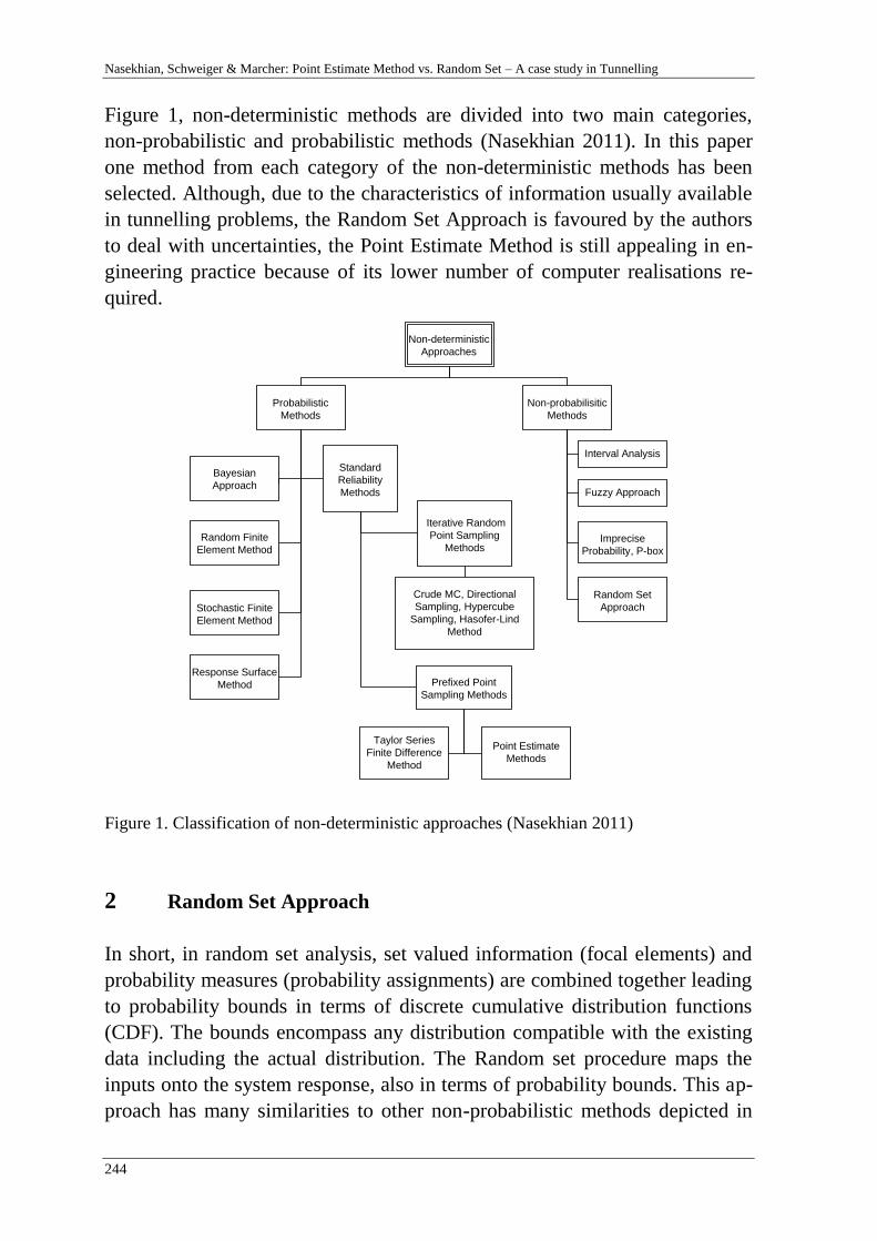
Nasekhian, Schweiger & Marcher: Point Estimate Method vs. Random Set – A case study in Tunnelling
244
Figure 1, non-deterministic methods are divided into two main categories,
non-probabilistic and probabilistic methods (Nasekhian 2011). In this paper
one method from each category of the non-deterministic methods has been
selected. Although, due to the characteristics of information usually available
in tunnelling problems, the Random Set Approach is favoured by the authors
to deal with uncertainties, the Point Estimate Method is still appealing in en-
gineering practice because of its lower number of computer realisations re-
quired.
Non-probabilisitic
Methods
Non-deterministic
Approaches
Probabilistic
Methods
Standard
Reliability
Methods
Bayesian
Approach
Random Finite
Element Method
Iterative Random
Point Sampling
Methods
Stochastic Finite
Element Method
Prefixed Point
Sampling Methods
Response Surface
Method
Crude MC, Directional
Sampling, Hypercube
Sampling, Hasofer-Lind
Method
Point Estimate
Methods
Taylor Series
Finite Difference
Method
Interval Analysis
Imprecise
Probability, P-box
Fuzzy Approach
Random Set
Approach
Figure 1. Classification of non-deterministic approaches (Nasekhian 2011)
2 Random Set Approach
In short, in random set analysis, set valued information (focal elements) and
probability measures (probability assignments) are combined together leading
to probability bounds in terms of discrete cumulative distribution functions
(CDF). The bounds encompass any distribution compatible with the existing
data including the actual distribution. The Random set procedure maps the
inputs onto the system response, also in terms of probability bounds. This ap-
proach has many similarities to other non-probabilistic methods depicted in
Moormann, Huber & Proske: Proceedings of the 10th International Probabilistic Workshop, Stuttgart 2012
245
Figure 1 such as the fuzzy set and p-box approach. For instance, both random
set and fuzzy set approaches are supported by set theory and interval analysis
that would be an integral part of their solution procedure. However, in Ran-
dom Set the independence of the individual information sources are preserved
while in the p-box approach a set is randomly taken by the Monte-Carlo pro-
cess at each simulation.
The random set is attractive in the sense that it enables engineers to consider
both “aleatory” and “epistemic” types of uncertainty. In tunnel engineering,
due to the linear nature of tunnel projects, usually very limited results from
investigation programs are available at the beginning of the design stage,
which leads to very sparse and scarce data. Consequently, the geotechnical
properties mostly appear in ranges without probability measures attributed
across the ranges. In such conditions, the random set approach is proposed
and preferable.
The applicability and efficiency of Random Set Finite Element Method (RS-
FEM) in geotechnical practice and tunnelling have been demonstrated in sev-
eral publications e.g. Peschl 2004, Schweiger et al. 2007, Nasekhian 2011,
Nasekhian & Schweiger 2011. The basics and the mathematical framework of
the Random Set are extensively discussed in the literature, e.g. Dubois and
Prade 1991 and Tonon et al. (2000), and are not repeated herein.
3 Point Estimate Method
The Point Estimate Method (PEM) is one of the probabilistic methods. In
brief, the probability distribution of input parameters is substituted by single
values and their respective predefined weights. The uncertainty model is
evaluated with the predefined sampling points and as a result, the statistical
moments of system responses that are of interest, are estimated.
This method is favourable in the sense of simplicity (from a practical point of
view) as well as its relatively low number of simulations, although there are
limitations and some of these are addressed in this paper.
In PEM, the Reliability analysis of a geotechnical problem in connection with
numerical models can be broken down into a limited number of deterministic
finite element calculations based on the number of predetermined points given
by the method. In this sense, PEM is similar to the Random Set Finite Ele-
ment Method. PEM is appealing in terms of the number of required realisa-
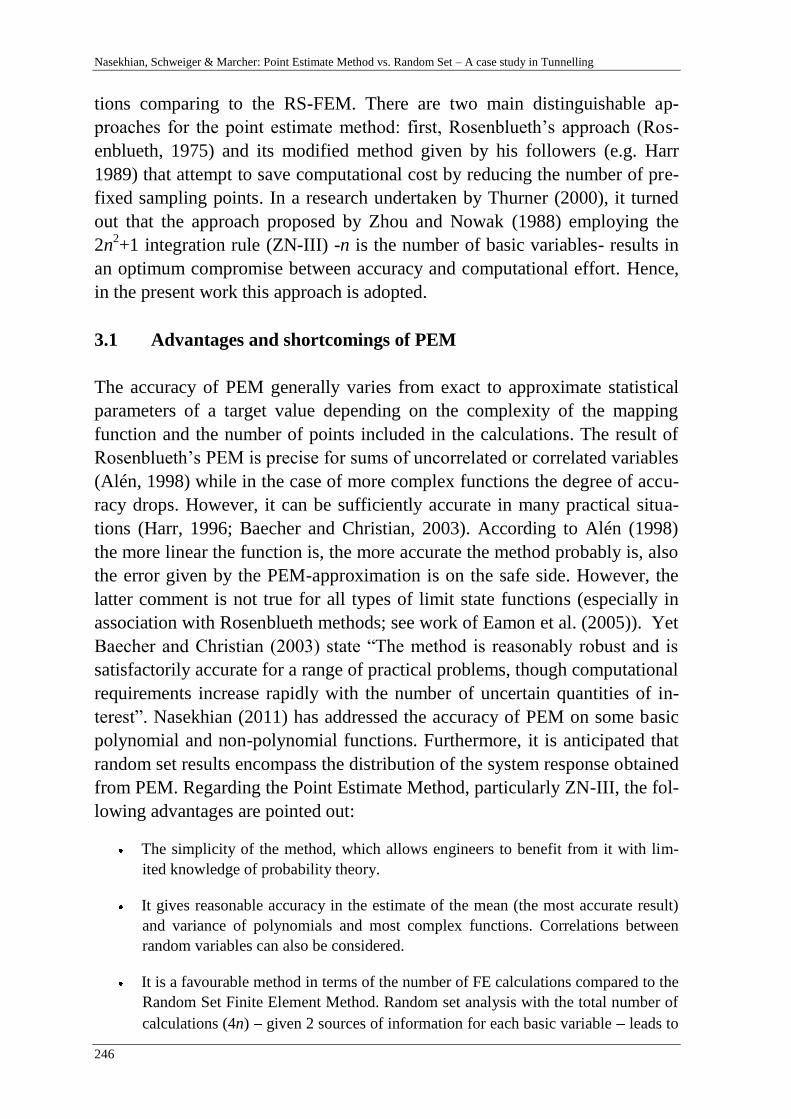
Nasekhian, Schweiger & Marcher: Point Estimate Method vs. Random Set – A case study in Tunnelling
246
tions comparing to the RS-FEM. There are two main distinguishable ap-
proaches for the point estimate method: first, Rosenblueth’s approach (Ros-
enblueth, 1975) and its modified method given by his followers (e.g. Harr
1989) that attempt to save computational cost by reducing the number of pre-
fixed sampling points. In a research undertaken by Thurner (2000), it turned
out that the approach proposed by Zhou and Nowak (1988) employing the
2n2+1 integration rule (ZN-III) -n is the number of basic variables- results in
an optimum compromise between accuracy and computational effort. Hence,
in the present work this approach is adopted.
3.1 Advantages and shortcomings of PEM
The accuracy of PEM generally varies from exact to approximate statistical
parameters of a target value depending on the complexity of the mapping
function and the number of points included in the calculations. The result of
Rosenblueth’s PEM is precise for sums of uncorrelated or correlated variables
(Alén, 1998) while in the case of more complex functions the degree of accu-
racy drops. However, it can be sufficiently accurate in many practical situa-
tions (Harr, 1996; Baecher and Christian, 2003). According to Alén (1998)
the more linear the function is, the more accurate the method probably is, also
the error given by the PEM-approximation is on the safe side. However, the
latter comment is not true for all types of limit state functions (especially in
association with Rosenblueth methods; see work of Eamon et al. (2005)). Yet
Baecher and Christian (2003) state “The method is reasonably robust and is
satisfactorily accurate for a range of practical problems, though computational
requirements increase rapidly with the number of uncertain quantities of in-
terest”. Nasekhian (2011) has addressed the accuracy of PEM on some basic
polynomial and non-polynomial functions. Furthermore, it is anticipated that
random set results encompass the distribution of the system response obtained
from PEM. Regarding the Point Estimate Method, particularly ZN-III, the fol-
lowing advantages are pointed out:
The simplicity of the method, which allows engineers to benefit from it with lim-
ited knowledge of probability theory.
It gives reasonable accuracy in the estimate of the mean (the most accurate result)
and variance of polynomials and most complex functions. Correlations between
random variables can also be considered.
It is a favourable method in terms of the number of FE calculations compared to the
Random Set Finite Element Method. Random set analysis with the total number of
calculations (4n) given 2 sources of information for each basic variable leads to
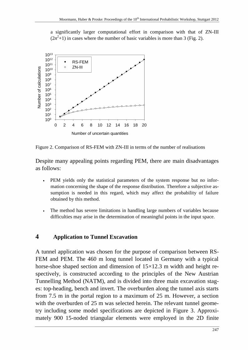
Moormann, Huber & Proske: Proceedings of the 10th International Probabilistic Workshop, Stuttgart 2012
247
a significantly larger computational effort in comparison with that of ZN-III
(2n2+1) in cases where the number of basic variables is more than 3 (Fig. 2).
Number of uncertain quantities
0 2 4 6 8 10 12 14 16 18 20
Num
ber
of
ca
lcula
tions
100
101
102
103
104
105
106
107
108
109
1010
1011
1012
1013
RS-FEM
ZN-III
Figure 2. Comparison of RS-FEM with ZN-III in terms of the number of realisations
Despite many appealing points regarding PEM, there are main disadvantages
as follows:
PEM yields only the statistical parameters of the system response but no infor-
mation concerning the shape of the response distribution. Therefore a subjective as-
sumption is needed in this regard, which may affect the probability of failure
obtained by this method.
The method has severe limitations in handling large numbers of variables because
difficulties may arise in the determination of meaningful points in the input space.
4 Application to Tunnel Excavation
A tunnel application was chosen for the purpose of comparison between RS-
FEM and PEM. The 460 m long tunnel located in Germany with a typical
horse-shoe shaped section and dimension of 15×12.3 m width and height re-
spectively, is constructed according to the principles of the New Austrian
Tunnelling Method (NATM), and is divided into three main excavation stag-
es: top-heading, bench and invert. The overburden along the tunnel axis starts
from 7.5 m in the portal region to a maximum of 25 m. However, a section
with the overburden of 25 m was selected herein. The relevant tunnel geome-
try including some model specifications are depicted in Figure 3. Approxi-
mately 900 15-noded triangular elements were employed in the 2D finite
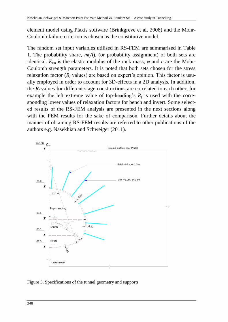
Nasekhian, Schweiger & Marcher: Point Estimate Method vs. Random Set – A case study in Tunnelling
248
element model using Plaxis software (Brinkgreve et al. 2008) and the Mohr-
Coulomb failure criterion is chosen as the constitutive model.
The random set input variables utilised in RS-FEM are summarised in Table
1. The probability share, m(A), (or probability assignment) of both sets are
identical. Erm is the elastic modulus of the rock mass, φ and c are the Mohr-
Coulomb strength parameters. It is noted that both sets chosen for the stress
relaxation factor (Rf values) are based on expert’s opinion. This factor is usu-
ally employed in order to account for 3D-effects in a 2D analysis. In addition,
the Rf values for different stage constructions are correlated to each other, for
example the left extreme value of top-heading’s Rf is used with the corre-
sponding lower values of relaxation factors for bench and invert. Some select-
ed results of the RS-FEM analysis are presented in the next sections along
with the PEM results for the sake of comparison. Further details about the
manner of obtaining RS-FEM results are referred to other publications of the
authors e.g. Nasekhian and Schweiger (2011).
Bolt l=6.0m, e=1.3m
Bolt l=4.0m, e=1.3m
CL
Top-Heading
Bench
Invert
+/-0.00
-25.0
-31.5
-35.1
-37.3
Units: meter
Ground surface near Portal
0.20
0.25
0.1
5
Figure 3. Specifications of the tunnel geometry and supports
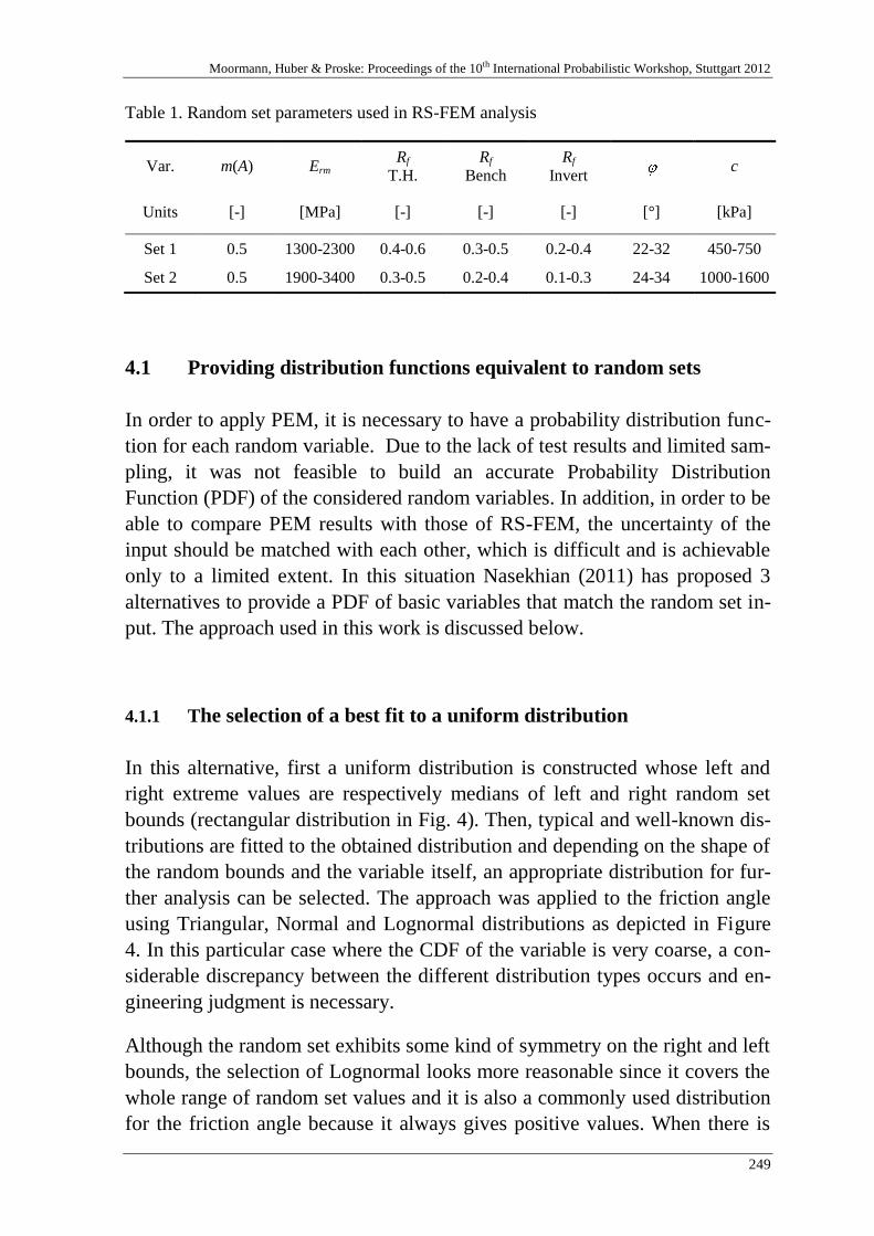
Moormann, Huber & Proske: Proceedings of the 10th International Probabilistic Workshop, Stuttgart 2012
249
Table 1. Random set parameters used in RS-FEM analysis
Var. m(A) Erm Rf
T.H.
Rf
Bench
Rf
Invert c
Units [-] [MPa] [-] [-] [-] [°] [kPa]
Set 1 0.5 1300-2300 0.4-0.6 0.3-0.5 0.2-0.4 22-32 450-750
Set 2 0.5 1900-3400 0.3-0.5 0.2-0.4 0.1-0.3 24-34 1000-1600
4.1 Providing distribution functions equivalent to random sets
In order to apply PEM, it is necessary to have a probability distribution func-
tion for each random variable. Due to the lack of test results and limited sam-
pling, it was not feasible to build an accurate Probability Distribution
Function (PDF) of the considered random variables. In addition, in order to be
able to compare PEM results with those of RS-FEM, the uncertainty of the
input should be matched with each other, which is difficult and is achievable
only to a limited extent. In this situation Nasekhian (2011) has proposed 3
alternatives to provide a PDF of basic variables that match the random set in-
put. The approach used in this work is discussed below.
4.1.1 The selection of a best fit to a uniform distribution
In this alternative, first a uniform distribution is constructed whose left and
right extreme values are respectively medians of left and right random set
bounds (rectangular distribution in Fig. 4). Then, typical and well-known dis-
tributions are fitted to the obtained distribution and depending on the shape of
the random bounds and the variable itself, an appropriate distribution for fur-
ther analysis can be selected. The approach was applied to the friction angle
using Triangular, Normal and Lognormal distributions as depicted in Figure
4. In this particular case where the CDF of the variable is very coarse, a con-
siderable discrepancy between the different distribution types occurs and en-
gineering judgment is necessary.
Although the random set exhibits some kind of symmetry on the right and left
bounds, the selection of Lognormal looks more reasonable since it covers the
whole range of random set values and it is also a commonly used distribution
for the friction angle because it always gives positive values. When there is
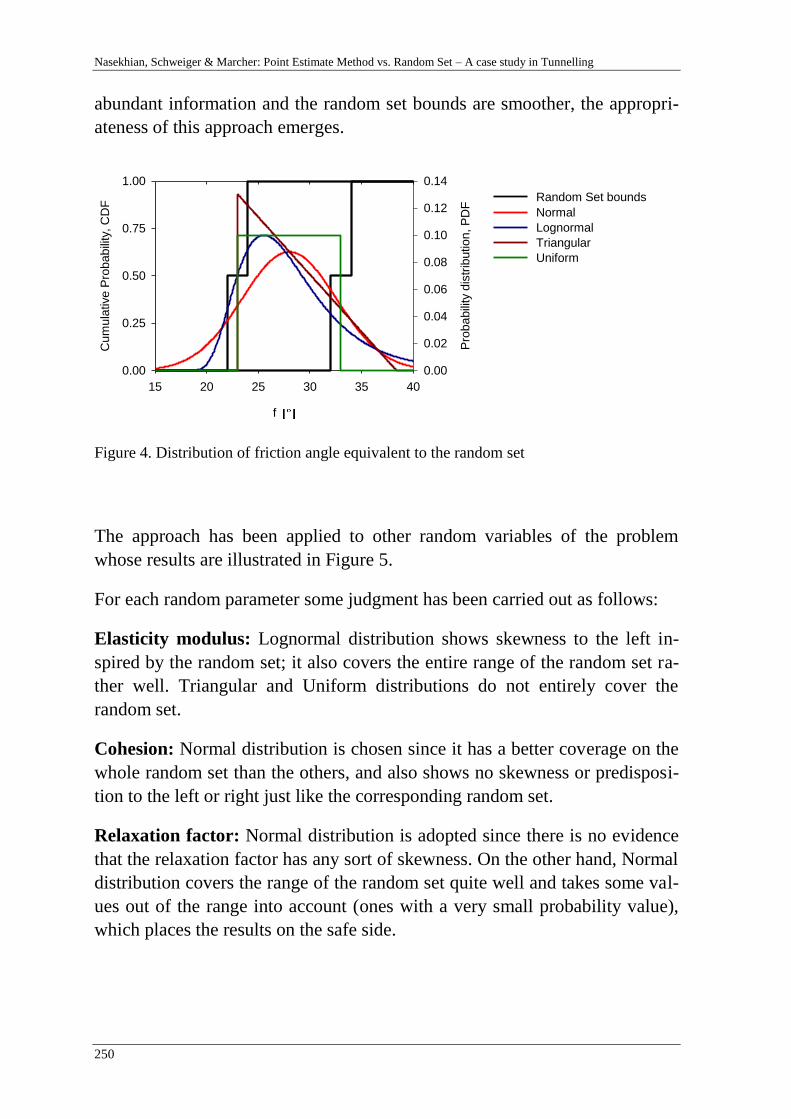
Nasekhian, Schweiger & Marcher: Point Estimate Method vs. Random Set – A case study in Tunnelling
250
abundant information and the random set bounds are smoother, the appropri-
ateness of this approach emerges.
f
15 20 25 30 35 40
Cum
ula
tive P
robabili
ty, C
DF
0.00
0.25
0.50
0.75
1.00
Pro
babili
ty d
istr
ibution, P
DF
0.00
0.02
0.04
0.06
0.08
0.10
0.12
0.14
Random Set bounds
Normal
Lognormal
Triangular
Uniform
Figure 4. Distribution of friction angle equivalent to the random set
The approach has been applied to other random variables of the problem
whose results are illustrated in Figure 5.
For each random parameter some judgment has been carried out as follows:
Elasticity modulus: Lognormal distribution shows skewness to the left in-
spired by the random set; it also covers the entire range of the random set ra-
ther well. Triangular and Uniform distributions do not entirely cover the
random set.
Cohesion: Normal distribution is chosen since it has a better coverage on the
whole random set than the others, and also shows no skewness or predisposi-
tion to the left or right just like the corresponding random set.
Relaxation factor: Normal distribution is adopted since there is no evidence
that the relaxation factor has any sort of skewness. On the other hand, Normal
distribution covers the range of the random set quite well and takes some val-
ues out of the range into account (ones with a very small probability value),
which places the results on the safe side.
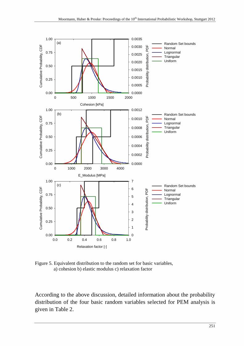
Moormann, Huber & Proske: Proceedings of the 10th International Probabilistic Workshop, Stuttgart 2012
251
Cohesion [kPa]
0 500 1000 1500 2000
Cum
ula
tive
Pro
ba
bili
ty, C
DF
0.00
0.25
0.50
0.75
1.00
Pro
ba
bili
ty d
istr
ibutio
n, P
DF
0.0000
0.0005
0.0010
0.0015
0.0020
0.0025
0.0030
0.0035
Random Set bounds
Normal
Lognormal
Triangular
Uniform
E_Modulus [MPa]
0 1000 2000 3000 4000
Cum
ula
tive
Pro
ba
bili
ty, C
DF
0.00
0.25
0.50
0.75
1.00
Pro
ba
bili
ty d
istr
ibutio
n, P
DF
0.0000
0.0002
0.0004
0.0006
0.0008
0.0010
0.0012
Random Set bounds
Normal
Lognormal
Triangular
Uniform
Relaxation factor [-]
0.0 0.2 0.4 0.6 0.8 1.0
Cum
ula
tive
Pro
ba
bili
ty, C
DF
0.00
0.25
0.50
0.75
1.00
Pro
ba
bili
ty d
istr
ibutio
n, P
DF
0
1
2
3
4
5
6
7
Random Set bounds
Normal
Lognormal
Triangular
Uniform
(a)
(b)
(c)
Figure 5. Equivalent distribution to the random set for basic variables,
a) cohesion b) elastic modulus c) relaxation factor
According to the above discussion, detailed information about the probability
distribution of the four basic random variables selected for PEM analysis is
given in Table 2.
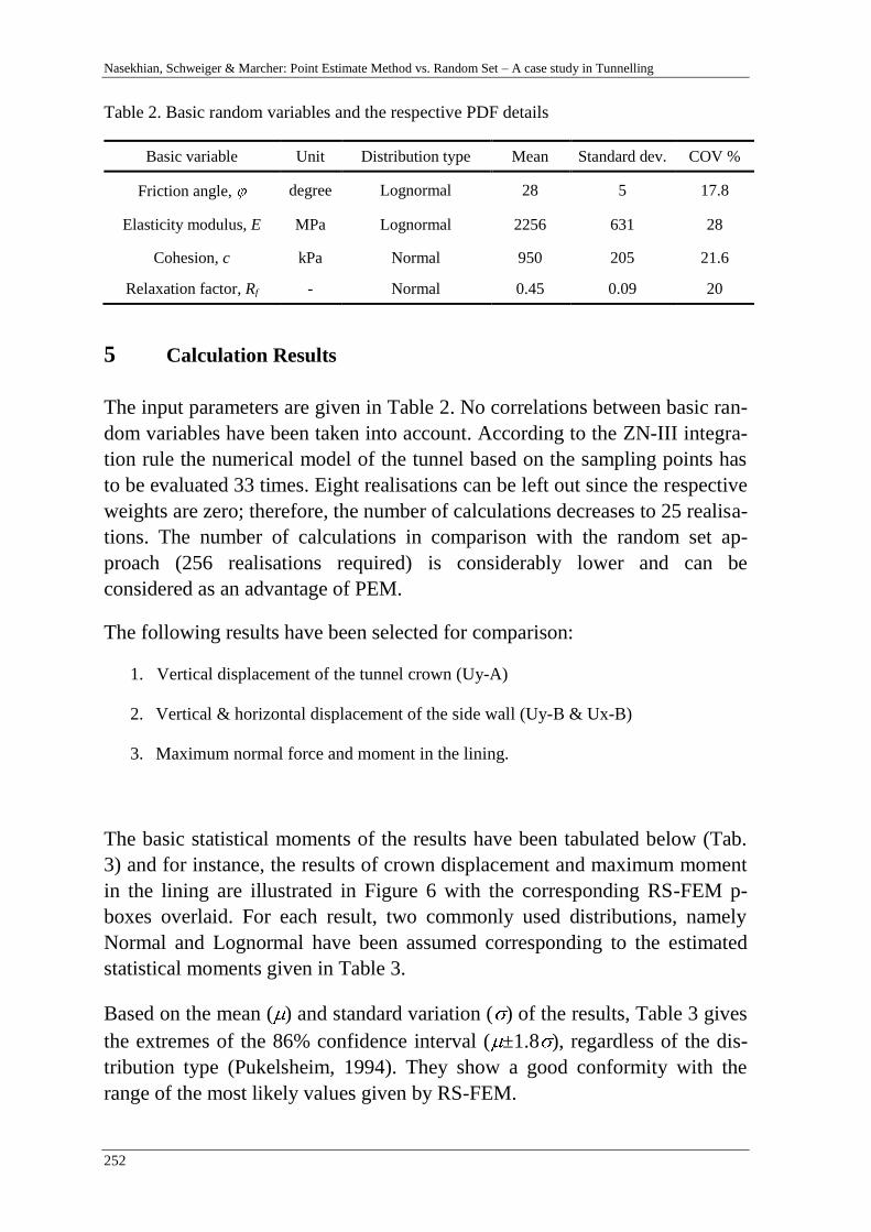
Nasekhian, Schweiger & Marcher: Point Estimate Method vs. Random Set – A case study in Tunnelling
252
Table 2. Basic random variables and the respective PDF details
Basic variable Unit Distribution type Mean Standard dev. COV %
Friction angle, degree Lognormal 28 5 17.8
Elasticity modulus, E MPa Lognormal 2256 631 28
Cohesion, c kPa Normal 950 205 21.6
Relaxation factor, Rf - Normal 0.45 0.09 20
5 Calculation Results
The input parameters are given in Table 2. No correlations between basic ran-
dom variables have been taken into account. According to the ZN-III integra-
tion rule the numerical model of the tunnel based on the sampling points has
to be evaluated 33 times. Eight realisations can be left out since the respective
weights are zero; therefore, the number of calculations decreases to 25 realisa-
tions. The number of calculations in comparison with the random set ap-
proach (256 realisations required) is considerably lower and can be
considered as an advantage of PEM.
The following results have been selected for comparison:
1. Vertical displacement of the tunnel crown (Uy-A)
2. Vertical & horizontal displacement of the side wall (Uy-B & Ux-B)
3. Maximum normal force and moment in the lining.
The basic statistical moments of the results have been tabulated below (Tab.
3) and for instance, the results of crown displacement and maximum moment
in the lining are illustrated in Figure 6 with the corresponding RS-FEM p-
boxes overlaid. For each result, two commonly used distributions, namely
Normal and Lognormal have been assumed corresponding to the estimated
statistical moments given in Table 3.
Based on the mean ( ) and standard variation ( ) of the results, Table 3 gives
the extremes of the 86% confidence interval ( ±1.8 ), regardless of the dis-
tribution type (Pukelsheim, 1994). They show a good conformity with the
range of the most likely values given by RS-FEM.
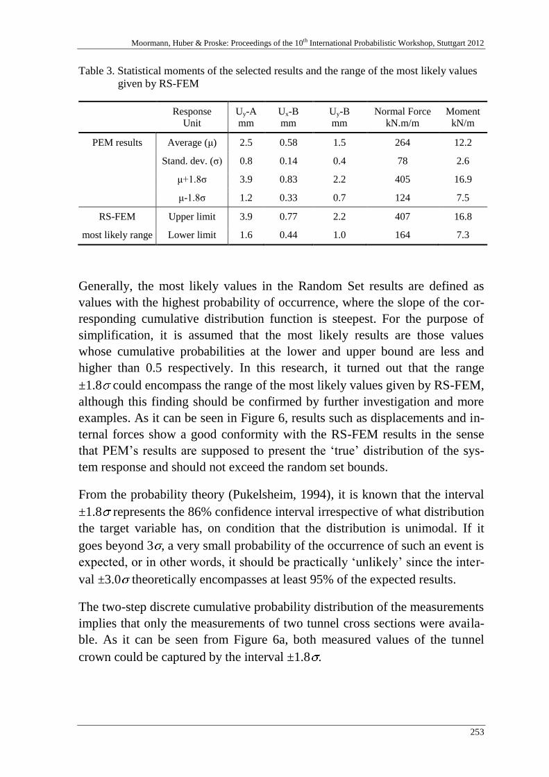
Moormann, Huber & Proske: Proceedings of the 10th International Probabilistic Workshop, Stuttgart 2012
253
Table 3. Statistical moments of the selected results and the range of the most likely values
given by RS-FEM
Response
Unit
Uy-A
mm
Ux-B
mm
Uy-B
mm
Normal Force
kN.m/m
Moment
kN/m
PEM results Average (μ) 2.5 0.58 1.5 264 12.2
Stand. dev. (σ) 0.8 0.14 0.4 78 2.6
μ+1.8σ 3.9 0.83 2.2 405 16.9
μ-1.8σ 1.2 0.33 0.7 124 7.5
RS-FEM Upper limit 3.9 0.77 2.2 407 16.8
most likely range Lower limit 1.6 0.44 1.0 164 7.3
Generally, the most likely values in the Random Set results are defined as
values with the highest probability of occurrence, where the slope of the cor-
responding cumulative distribution function is steepest. For the purpose of
simplification, it is assumed that the most likely results are those values
whose cumulative probabilities at the lower and upper bound are less and
higher than 0.5 respectively. In this research, it turned out that the range
±1.8 could encompass the range of the most likely values given by RS-FEM,
although this finding should be confirmed by further investigation and more
examples. As it can be seen in Figure 6, results such as displacements and in-
ternal forces show a good conformity with the RS-FEM results in the sense
that PEM’s results are supposed to present the ‘true’ distribution of the sys-
tem response and should not exceed the random set bounds.
From the probability theory (Pukelsheim, 1994), it is known that the interval
±1.8 represents the 86% confidence interval irrespective of what distribution
the target variable has, on condition that the distribution is unimodal. If it
goes beyond 3 , a very small probability of the occurrence of such an event is
expected, or in other words, it should be practically ‘unlikely’ since the inter-
val ±3.0 theoretically encompasses at least 95% of the expected results.
The two-step discrete cumulative probability distribution of the measurements
implies that only the measurements of two tunnel cross sections were availa-
ble. As it can be seen from Figure 6a, both measured values of the tunnel
crown could be captured by the interval ±1.8 .
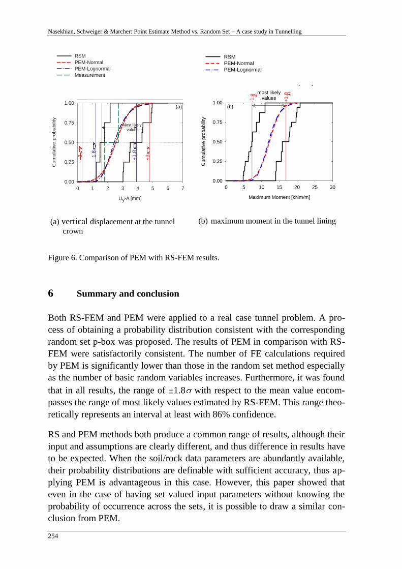
Nasekhian, Schweiger & Marcher: Point Estimate Method vs. Random Set – A case study in Tunnelling
254
Uy-A [mm]
0 1 2 3 4 5 6 7
Cum
ula
tive p
rob
abili
ty
0.00
0.25
0.50
0.75
1.00
Uy-B [mm]
0 1 2 3 4 5
Cum
ula
tive
pro
ba
bili
ty
0.00
0.25
0.50
0.75
1.00
Ux-B [mm]
0.0 0.5 1.0 1.5 2.0
Cum
ula
tive p
roba
bili
ty
0.00
0.25
0.50
0.75
1.00
+1.8
1.8
+33
+1.8
1.8
+33
+1.8
1.8
+33
RS-FEM Quality indicator
RS-FEM Quality indicator
PEM Quality indicator
PEM Quality indicator
PEM Quality indicator
RSM
PEM-Normal
PEM-Lognormal
Measurement
RSM
PEM-Normal
PEM-Lognormal
Measurement
RS-FEM Quality indicator
Most likely values
Most likely values
(a)
(c)
(b)
Most likely values
RSM
PEM-Normal
PEM-Lognormal
Measurement
Maximum normal force [kN/m]
100 200 300 400 500 600 700
Cum
ula
tive
pro
ba
bili
ty, C
DF
0.00
0.25
0.50
0.75
1.00
Pro
ba
bili
ty d
istr
ibutio
n, P
DF
0.000
0.001
0.002
0.003
0.004
0.005
0.006
RSM
PEM-Normal
PEM-Lognormal
PEM-Shifted lognormal
-1.8
+1
.8
most likelyvalues
FOS [-]
0 2 4 6 8 10 12 14
Cum
ula
tive
pro
ba
bili
ty
0.00
0.25
0.50
0.75
1.00
RSM
PEM-Normal
PEM-Lognormal
PEM-Shifted lognormal
-1.8
+1
.8
most likelyvalues
Maximum Moment [kNm/m]
0 5 10 15 20 25 30
Cum
ula
tive
pro
ba
bili
ty
0.00
0.25
0.50
0.75
1.00
RSM
PEM-Normal
PEM-Lognormal
-1.8
+1
.8most likelyvalues
(a)
(b)
(c)
Maximum normal force [kN/m]
100 200 300 400 500 600 700
Cum
ula
tive p
robabili
ty, C
DF
0.00
0.25
0.50
0.75
1.00
Pro
babili
ty d
istr
ibution, P
DF
0.000
0.001
0.002
0.003
0.004
0.005
0.006
RSM
PEM-Normal
PEM-Lognormal
PEM-Shifted lognormal
-1.8
+1.8
most likelyvalues
FOS [-]
0 2 4 6 8 10 12 14
Cum
ula
tive p
robabili
ty
0.00
0.25
0.50
0.75
1.00
RSM
PEM-Normal
PEM-Lognormal
PEM-Shifted lognormal
-1.8
+1.8
most likelyvalues
Maximum Moment [kNm/m]
0 5 10 15 20 25 30
Cum
ula
tive p
robabili
ty
0.00
0.25
0.50
0.75
1.00
RSM
PEM-Normal
PEM-Lognormal
-1.8
+1.8most likely
values
(a)
(b)
(c)
Uy-A [mm]
0 1 2 3 4 5 6 7
Cum
ula
tive p
rob
abili
ty
0.00
0.25
0.50
0.75
1.00
Uy-B [mm]
0 1 2 3 4 5
Cum
ula
tive
pro
ba
bili
ty
0.00
0.25
0.50
0.75
1.00
Ux-B [mm]
0.0 0.5 1.0 1.5 2.0
Cum
ula
tive p
roba
bili
ty
0.00
0.25
0.50
0.75
1.00
+1
.8
1.8
+33
+1
.8
1.8
+33
+1.8
1.8
+33
RS-FEM Quality indicator
RS-FEM Quality indicator
PEM Quality indicator
PEM Quality indicator
PEM Quality indicator
RSM
PEM-Normal
PEM-Lognormal
Measurement
RSM
PEM-Normal
PEM-Lognormal
Measurement
RS-FEM Quality indicator
Most likely values
Most likely values
(a)
(c)
(b)
Most likely values
RSM
PEM-Normal
PEM-Lognormal
Measurement
(a) vertical displacement at the tunnel
crown
(b) maximum moment in the tunnel lining
Figure 6. Comparison of PEM with RS-FEM results.
6 Summary and conclusion
Both RS-FEM and PEM were applied to a real case tunnel problem. A pro-
cess of obtaining a probability distribution consistent with the corresponding
random set p-box was proposed. The results of PEM in comparison with RS-
FEM were satisfactorily consistent. The number of FE calculations required
by PEM is significantly lower than those in the random set method especially
as the number of basic random variables increases. Furthermore, it was found
that in all results, the range of ±1.8 with respect to the mean value encom-
passes the range of most likely values estimated by RS-FEM. This range theo-
retically represents an interval at least with 86% confidence.
RS and PEM methods both produce a common range of results, although their
input and assumptions are clearly different, and thus difference in results have
to be expected. When the soil/rock data parameters are abundantly available,
their probability distributions are definable with sufficient accuracy, thus ap-
plying PEM is advantageous in this case. However, this paper showed that
even in the case of having set valued input parameters without knowing the
probability of occurrence across the sets, it is possible to draw a similar con-
clusion from PEM.

Moormann, Huber & Proske: Proceedings of the 10th International Probabilistic Workshop, Stuttgart 2012
255
7 References
[1] Alén, C. (1998) On Probability in Geotechnics: Random Calculation Models Exem-
plified on Slope Stability Analysis and Ground-Superstructure Interaction. Depart-
ment of Geotechnical Engineering, Chalmers University of Technology. Dissertation.
[2] Baecher, G.B.; Christian, J.T. (2003) Reliability and Statistics in Geotechnical Engi-
neering. New York: Wiley & Sons.
[3] Brinkgreve, R.B.J.; Broere, W. (2008) PLAXIS, Finite element code for soil and
rock analyses, users manual. Version 9, Rotterdam: Balkema.
[4] Dubois, D.; Prade, H. (1991) Random sets and fuzzy interval analysis. Fuzzy Sets
and Systems, Vol. 42, 87-101.
[5] Eamon, C.D.; Thompson, M.; Liu, Z. (2005) Evaluation of accuracy and efficiency
of some simulation and sampling methods in structural reliability analysis. Structural
Safety, Vol. 27, No. 4, 356-392.
[6] Harr, M.E. (1989) Probabilistic estimates for multivariate analyses. Applied Mathe-
matical Modelling, Vol. 13, No. 5, 313-318.
[7] Nasekhian, A.; Schweiger, H.F. (2011) Random Set Finite Element Method applica-
tion to tunnelling. Int. J. Reliability and Safety, Inderscience Publishers, 5(3/4), 299-
319
[8] Nasekhian, A. (2011) Application of Non-probabilistic and Probabilistic Concepts in
Finite Element Analysis of Tunnelling. Institute for Soil Mechanics and Foundation
Engineering, Graz University of Technology, Dissertation.
[9] Peschl, G.M. (2004) Reliability Analyses in Geotechnics with the Random Set Finite
Element Method. Graz University of Technology, Dissertation.
[10] Pukelsheim, F. (1994) The Three Sigma Rule. The American Statistician, Vol. 48,
No. 2 , 88-91.
[11] Rosenblueth, E. (1975) Point estimates for probability moments. Proc. Nat. Acad.
Sci. USA, Vol. 72, No. 10, 3812-3814.
[12] Schweiger, H.F.; Peschl, G.M.; Pöttler, R. (2007) Application of the random set finite
element method for analysing tunnel excavation. Georisk 1, S. 43-56.
[13] Thurner, R. (2000) Probabilistische Untersuchungen in der Geotechnik mittels De-
terministischer Finite Elemente-Methode, Institut für Bodenmechanik und Grundbau,
TU-Graz, Dissertation.
[14] Tonon, F.; Bernardini, A.; Mammino, A. (2000) Reliability analysis of rock mass
response by means of Random Set Theory. Reliability Engineering & System Safety,
Vol. 70, No. 3, 263-282.

Nasekhian, Schweiger & Marcher: Point Estimate Method vs. Random Set – A case study in Tunnelling
256
[15] Zhou, J.; Nowak, A.S. (1988) Integration formulas to evaluate functions of random
variables. Structural safety, Vol. 5, No. 4, 267-284.

Moormann, Huber & Proske: Proceedings of the 10th International Probabilistic Workshop, Stuttgart 2012
257
Classification of warning systems for natural
hazards
Martina Sättele, Michael Bründl (1), Daniel Straub (2)
(1) Research Group Avalanche Dynamics and Risk Management, WSL Insti-
tute for Snow and Avalanche Research SLF, Davos
(2) Engineering Risk Analysis Group, TU München, Munich
Abstract: Intensified efforts are being made to establish warning systems as
efficient components of an integrated risk management strategy for natural
hazards. While testing and reliability analyses are well established procedures
for active protection measures such as dams, rockfall nets and galleries, meth-
ods and conventions for evaluating the reliability of warning systems are lack-
ing. To incorporate warning systems as standard measures of an integrated risk
management strategy for natural hazards, their reliability must be quantifiable.
The aim of this contribution is to establish appropriate reliability quantification
methods for warning systems by classifying them according to characteristics
relevant to assessing their reliability. Firstly, chief natural hazard processes in
Switzerland in need of warning systems are selected and system relevant pro-
cess characteristics such as the role of the geographical disposition of the event
site, trigger events and dynamic process parameters are clarified. In three ex-
amples the influence of the process characteristics on the monitoring possibili-
ties with respect to the system lead time is illustrated. A system classification is
suggested, which classifies the systems in i) threshold systems, ii) expert sys-
tems and iii) model-based expert systems. The classification is applied to 52
warning systems in Switzerland and for each system class typical characteris-
tics such as the lead time, the geographical range, the degree of human influ-
ence vs. technical influence and direct vs. indirect monitoring possibilities are
identified. The classification allows a structured identification of reliability cri-
teria for each class and is a first step towards development of a method for
quantifying the reliability of warning systems for natural hazards.

A typical publication for the 10th International Probabilistic Workshop
258
1 Introduction
Integrated risk management aims to mitigate the risk caused by natural haz-
ards to persons, animals, infrastructures and to achieve protection goals
through the application of approved mitigation measures. Thereby, risk to an
object associated with a scenario is a function of [3]:
probability of occurrence of scenario ,
presence probability of object in scenario ,
vulnerability of object in scenario j,
value of object .
Warning systems mitigate the overall risk level by reducing and with suf-
ficient warning time can be reduced [10]. One of the first automated warn-
ing system in Switzerland is the snow avalanche detection system in
“Mahnkinn”, commissioned by a railway company in 1953 [20]. Since then,
the use of viable warning systems has increased considerably, and warning
systems have been established by a number of different institutions according
to different needs specific to various natural hazard processes all over Swit-
zerland. To date the systems are often installed as prototypes where technical
developments are tailored to specific projects and there is little standardisation
between systems [11]. In order to incorporate warning systems as standard
measures in an integrated risk management strategy for natural hazards, their
reliability must be quantifiable. Warning systems are complex technical sys-
tems and to efficiently access their reliability requires an holistic system ap-
proach considering the system design and the technical failures as well as the
natural hazard process characteristics and the human influences. A system
classification is the first step towards such a method, since it allows the identi-
fication of system reliability criteria in a structured manner. At present a rec-
ognized classification of this kind does not exist.
Glantz [8] discusses system types and classification criteria, but argues that
even a simple definition for the term warning system is not practical and thus
limits the system diversity, the space for interpretations and the opportunity
for future system advancements. The Swiss Federal Office for Civil Protec-
tion distinguishes between warning, which is a notification to authorities, and
alarm, which is issued directly to general public [6]. According to the United
Nations Office for Disaster Risk Reduction [14], a warning system is “a set of
capacities needed to generate and disseminate timely and meaningful warning
information to enable individuals, communities and organizations threatened
by a hazard to prepare and to act appropriately and in sufficient time to reduce

Moormann, Huber & Proske: Proceedings of the 10th International Probabilistic Workshop, Stuttgart 2012
259
the possibility of harm or loss”. Monitoring is a part of warning, but it does
not include automatic issued warning possibilities and is thus no warning sys-
tem [8]. Bell et al. [2] classify warning systems in monitoring, expert and
alarm systems, but emphasize that a sharp system classification is not conven-
ient. These approaches and ideas are the starting point for the development of
the classification proposed in this paper.
2 Hazard processes and warning systems in Switzerland
The geography of Switzerland implicates that natural hazards often involve
water or mass movement processes. The landscape is characterised through
rivers and more than 1500 lakes, and the Alps cover 60% of the country
[22,23]. The most frequent events in Switzerland are forest fires, earthquakes,
floods, (thunder) storms, rock and snow avalanches, debris flows, rock/ block
and ice falls, permanent landslides, flash floods and glacier lake outburst
floods (GLOF) [21]. Floods, hail and storm have been causing the highest
property damages since 1990 [13], while the number of flood, debris flow,
landslide and rockfall damages between 1972 and 2007 were dominated by
six major flood events [12]. They caused over 50% of the total damages rec-
orded and were mainly triggered through long-lasting rain fall [12]. Perma-
nent landslides, debris flows and rockfalls caused 64 fatalities while floods
caused 46 deaths between 1972 and 2007 (Rockfall events have only be rec-
orded since 2002). Snow avalanches have the highest fatality rate with about
25 deaths each winter, of which a great number are self-inflicted by moun-
taineers and off-piste skiers [12].
The range of warning systems identified in four Cantons of Switzerland
(Bernese Oberland, Grison, Ticino and Valais) mainly covers the variety of
hazard processes identified (Figure 1). The documentation and analysis of
these 52 active warning systems is the basis for the classification. Thereof are
four systems operated by specialist departments on a national scale (Federal
Office for the Environment (FOEN) - flood, MeteoSchweiz - meteo hazards,
Swiss Seismological Service (SED) - earthquake, WSL Institute for Snow and
Avalanche Research SLF - snow avalanches). The identified systems are in-
stalled for ten different hazards processes and classified following the sugges-
tion from Dikau and Weichselgartner [4].
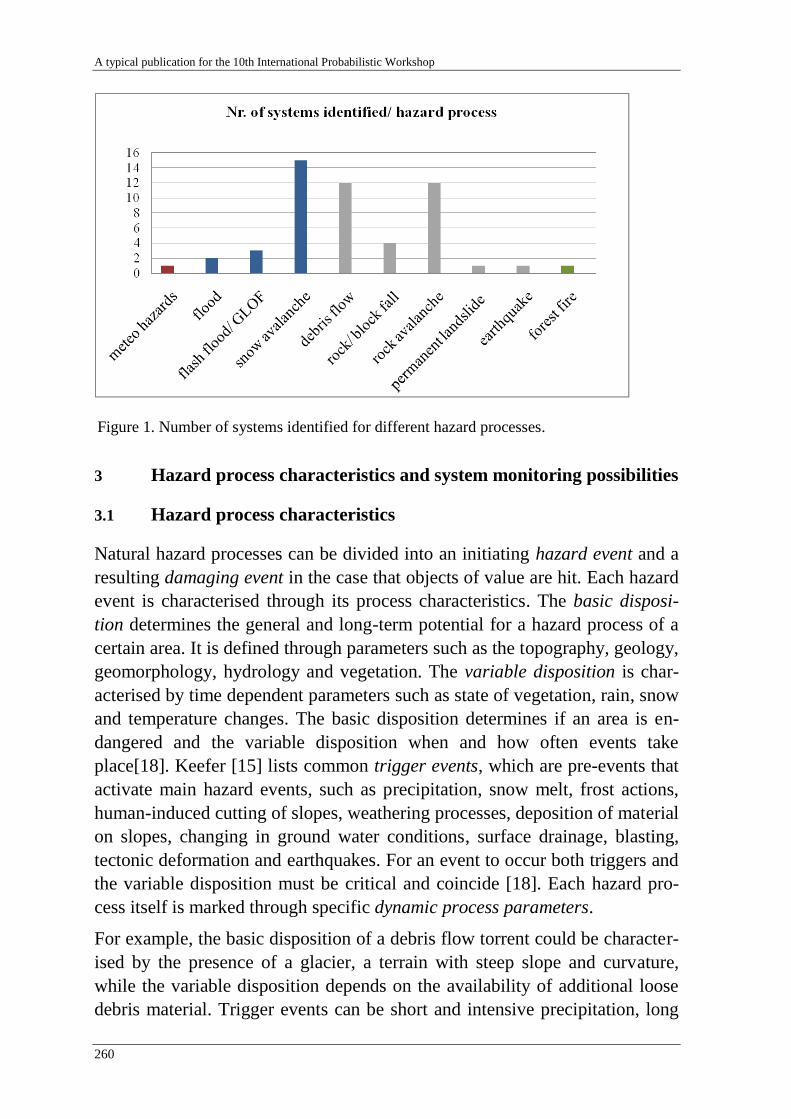
A typical publication for the 10th International Probabilistic Workshop
260
3 Hazard process characteristics and system monitoring possibilities
3.1 Hazard process characteristics
Natural hazard processes can be divided into an initiating hazard event and a
resulting damaging event in the case that objects of value are hit. Each hazard
event is characterised through its process characteristics. The basic disposi-
tion determines the general and long-term potential for a hazard process of a
certain area. It is defined through parameters such as the topography, geology,
geomorphology, hydrology and vegetation. The variable disposition is char-
acterised by time dependent parameters such as state of vegetation, rain, snow
and temperature changes. The basic disposition determines if an area is en-
dangered and the variable disposition when and how often events take
place[18]. Keefer [15] lists common trigger events, which are pre-events that
activate main hazard events, such as precipitation, snow melt, frost actions,
human-induced cutting of slopes, weathering processes, deposition of material
on slopes, changing in ground water conditions, surface drainage, blasting,
tectonic deformation and earthquakes. For an event to occur both triggers and
the variable disposition must be critical and coincide [18]. Each hazard pro-
cess itself is marked through specific dynamic process parameters.
For example, the basic disposition of a debris flow torrent could be character-
ised by the presence of a glacier, a terrain with steep slope and curvature,
while the variable disposition depends on the availability of additional loose
debris material. Trigger events can be short and intensive precipitation, long
Figure 1. Number of systems identified for different hazard processes.
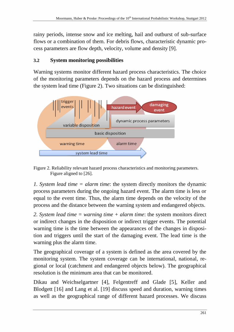
Moormann, Huber & Proske: Proceedings of the 10th International Probabilistic Workshop, Stuttgart 2012
261
rainy periods, intense snow and ice melting, hail and outburst of sub-surface
flows or a combination of them. For debris flows, characteristic dynamic pro-
cess parameters are flow depth, velocity, volume and density [9].
3.2 System monitoring possibilities
Warning systems monitor different hazard process characteristics. The choice
of the monitoring parameters depends on the hazard process and determines
the system lead time (Figure 2). Two situations can be distinguished:
Figure 2. Reliability relevant hazard process characteristics and monitoring parameters.
Figure aligned to [26].
1. System lead time = alarm time: the system directly monitors the dynamic
process parameters during the ongoing hazard event. The alarm time is less or
equal to the event time. Thus, the alarm time depends on the velocity of the
process and the distance between the warning system and endangered objects.
2. System lead time = warning time + alarm time: the system monitors direct
or indirect changes in the disposition or indirect trigger events. The potential
warning time is the time between the appearances of the changes in disposi-
tion and triggers until the start of the damaging event. The lead time is the
warning plus the alarm time.
The geographical coverage of a system is defined as the area covered by the
monitoring system. The system coverage can be international, national, re-
gional or local (catchment and endangered objects below). The geographical
resolution is the minimum area that can be monitored.
Dikau and Weichselgartner [4], Felgentreff and Glade [5], Keller and
Blodgett [16] and Lang et al. [19] discuss speed and duration, warning times
as well as the geographical range of different hazard processes. We discuss
A typical publication for the 10th International Probabilistic Workshop
262
the influence of process characteristics on the system monitoring parameters
in the following three examples.
The Swiss Federal Institute for Forest, Snow and Landscape Research (WSL)
operates a local debris flow warning system at Illgraben in Canton Valais.
The system aims to detect ongoing events by monitoring specific dynamic
process parameters. Geophones and radars are controlled by a logger, which
initiates an alarm if certain thresholds for ground motion and water level are
exceeded. This alarm automatically triggers acoustic and optic signals to warn
the population in the catchment area. Additionally, authorities responsible for
managing the hazard are informed directly and data of the event is stored in a
database. Here the lead time is equal to the alarm time [1].
A local rock avalanche system was installed at Preonzo in Canton Ticino
which was able to provide sufficient warning time of an event in May 2012.
Prediction of the release time was possible through monitoring the variable
disposition [7]. Rock avalanches, although spontaneous events [24], have typ-
ically long warning times, as they start with visible cracks, move slowly and
accelerate over time [17]. In Preonzo extensometers and a theodolite were
installed to directly measure pre-failure movements of the rock-mass at regu-
lar intervals. An alarm was sent to the authorities and geologists whenever a
specific velocity threshold was exceeded. The decision about further actions
was made by the experts after analysing the input data. The acceleration of the
rock-mass was evaluated in simple models to predict critical failure. Final
evacuation decisions were made based on these models and information
drawn from indirect rain data. The lead time incorporated the warning time.
The national avalanche warning system operated by SLF issues information
about the avalanche danger level for specific alpine regions and the Jura daily
at 5pm as forecast for the following day during the winter. Avalanche fore-
casters use measurements of snow height, amount of fresh snow, air and snow
temperature, solar radiation, wind direction and wind speed. This data inputs
are crucial for judging the snowpack stability and the release of avalanches,
because they affect the variable disposition. The data are collected from 180
automatic measuring stations and observers in the field. In addition, experts
consult meteorological forecasts and complex snowpack models for generat-
ing two public and daily avalanche bulletins. The lead time incorporates the
warning time [25].
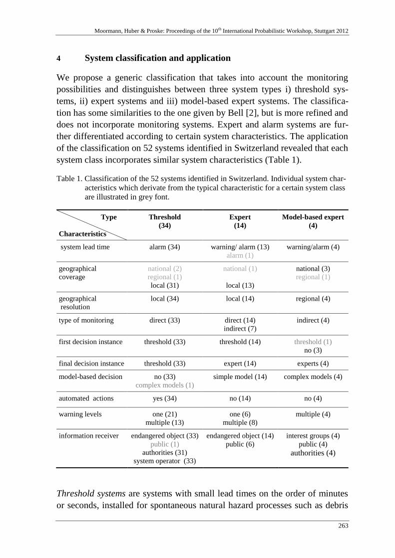
Moormann, Huber & Proske: Proceedings of the 10th International Probabilistic Workshop, Stuttgart 2012
263
4 System classification and application
We propose a generic classification that takes into account the monitoring
possibilities and distinguishes between three system types i) threshold sys-
tems, ii) expert systems and iii) model-based expert systems. The classifica-
tion has some similarities to the one given by Bell [2], but is more refined and
does not incorporate monitoring systems. Expert and alarm systems are fur-
ther differentiated according to certain system characteristics. The application
of the classification on 52 systems identified in Switzerland revealed that each
system class incorporates similar system characteristics (Table 1).
Table 1. Classification of the 52 systems identified in Switzerland. Individual system char-
acteristics which derivate from the typical characteristic for a certain system class
are illustrated in grey font.
Type
Characteristics
Threshold
(34)
Expert
(14)
Model-based expert
(4)
system lead time alarm (34) warning/ alarm (13)
alarm (1)
warning/alarm (4)
geographical
coverage
national (2)
regional (1)
local (31)
national (1)
local (13)
national (3)
regional (1)
geographical
resolution
local (34) local (14) regional (4)
type of monitoring direct (33) direct (14)
indirect (7)
indirect (4)
first decision instance threshold (33) threshold (14) threshold (1)
no (3)
final decision instance threshold (33) expert (14) experts (4)
model-based decision no (33)
complex models (1)
simple model (14) complex models (4)
automated actions yes (34) no (14) no (4)
warning levels one (21)
multiple (13)
one (6)
multiple (8)
multiple (4)
information receiver endangered object (33)
public (1)
authorities (31)
system operator (33)
endangered object (14)
public (6)
interest groups (4)
public (4)
authorities (4)
Threshold systems are systems with small lead times on the order of minutes
or seconds, installed for spontaneous natural hazard processes such as debris
A typical publication for the 10th International Probabilistic Workshop
264
flows, snow avalanches, rock/ block and ice falls, GLOFs and flash flood. The
geographical coverage and resolution is local. Dynamic process parameters
are directly monitored in the field. A threshold determines if an alarm is is-
sued e.g. in the form of colored or flashing lights or acoustic signals. Alarm
signals are automatically provided in one or multiple states of alarm to the
endangered objects, authorities and system operators.
Expert systems are installed for processes with longer lead times such as rock
avalanches and permanent landslides and have lead times on the order of
minutes to years. The systems installed are site specific and thus the geo-
graphical coverage and resolution of the systems is local. The parameters
monitored in the variable disposition are direct changes similar to the real
process parameters. The alarm is not issued automatically or with direct sig-
nals. Experts decide on necessary action plans by evaluating the monitored
data and by using simple models. In addition, data is collected from parame-
ters that are indirectly related to the process such as rain data. In most cases,
systems include different alarm levels and the data is made available only to
those responsible for managing natural hazards. For systems in Canton Ticino
all data are collected on a server and provided to the general public on a web-
site.
Model-based expert systems aim to make spontaneous hazard processes pre-
dictable. The alarm time is complemented with a warning time and hence a
lead time in the range of hours and days is reached. Immense sensor networks
offer national or regional system coverage. The input data are mainly gained
through indirect monitoring parameters influencing the variable disposition
and trigger data. They are further processed in complex models and resulting
in final products (e.g. bulletins) published on a regular base for general public
and affected institutions.
Each system class can be described though a typical system design which is
influenced by the identified characteristics. The design describes the
monitoring choice, the decision instances and their tresholds, expert and
model dependencies, data management and alternatives for implementing
measures of the integrated risk managment strategy (Figure 3).
Five out of 52 systems do not explicitly fit into one system class. The national
SED earthquake detection system is a typical example of such a system. By
counting the number of instances in which the system complies with the char-
acteristics of any class, the appropriate class can be identified. Thus, the SED
system is classified as a threshold system, which is based on complex models
covering a national area. Another edge case system in the threshold system
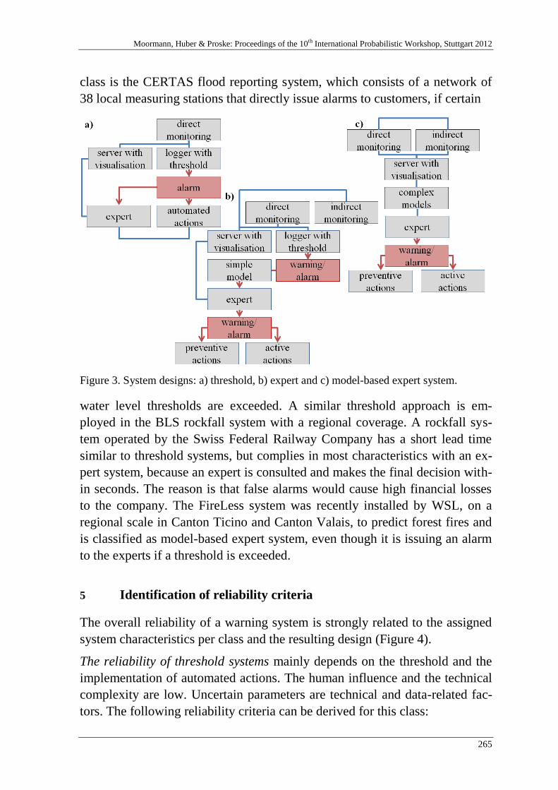
Moormann, Huber & Proske: Proceedings of the 10th International Probabilistic Workshop, Stuttgart 2012
265
class is the CERTAS flood reporting system, which consists of a network of
38 local measuring stations that directly issue alarms to customers, if certain
Figure 3. System designs: a) threshold, b) expert and c) model-based expert system.
water level thresholds are exceeded. A similar threshold approach is em-
ployed in the BLS rockfall system with a regional coverage. A rockfall sys-
tem operated by the Swiss Federal Railway Company has a short lead time
similar to threshold systems, but complies in most characteristics with an ex-
pert system, because an expert is consulted and makes the final decision with-
in seconds. The reason is that false alarms would cause high financial losses
to the company. The FireLess system was recently installed by WSL, on a
regional scale in Canton Ticino and Canton Valais, to predict forest fires and
is classified as model-based expert system, even though it is issuing an alarm
to the experts if a threshold is exceeded.
5 Identification of reliability criteria
The overall reliability of a warning system is strongly related to the assigned
system characteristics per class and the resulting design (Figure 4).
The reliability of threshold systems mainly depends on the threshold and the
implementation of automated actions. The human influence and the technical
complexity are low. Uncertain parameters are technical and data-related fac-
tors. The following reliability criteria can be derived for this class:

A typical publication for the 10th International Probabilistic Workshop
266
Figure 4. System types and the influence of reliability relevant characteristics on the sys-
tem reliability.
The monitoring of the correct dynamic process parameters is ensured through the
right choice of sensor type, redundancies and their ideal position and fixation.
A suitable threshold value should be chosen. A high threshold leads to missed
events and a low leads to false alarms.
The logger is functional. Power supply at remote sites is required, technical failure
is reduced to a minimum and communicated automatically.
The alarm transmission from the detection area to the endangered objectives is reli-
able, ideally redundant and controlled.
The functionality of the alarm facilities/ equipment is ensured and controlled.
The technical complexity and the number of interfaces between the system compo-
nents are kept to a minimum.
The reliability of expert systems is mainly influenced by the predefined
threshold and the decisions of the experts. Automated actions are not directly
implemented and the technical complexity is moderate. Uncertain parameters
are technical, human, data-related and organisational factors. The detection of
an event depends on the same reliability criteria as for the threshold system,
but is also dependent on the following criteria:
The data is transmitted to a server and made available to the experts.
The experts experience is high and their risk attitude neither too high nor too low.
The quality of models used is high and the indirect data are interpreted correctly.
Preventive and active actions are implemented in a timely manner.
The endangered objects are reached in a timely manner.
Moormann, Huber & Proske: Proceedings of the 10th International Probabilistic Workshop, Stuttgart 2012
267
The reliability of model-based expert systems is independent from thresholds
and the implementation of automated actions, but incorporates high human
influences, complex models and a high technical complexity. Uncertain pa-
rameters are technical, human, data-related, organisational- and standardisa-
tion-related factors. In addition to the factors illustrated above further criteria
are relevant for the system reliability:
Networks of several hundred sensors require a complex data management e.g. re-
dundant servers and clear work and decision processes.
The data format and measuring stations should be standardised, to minor the influ-
ence of measuring failures, because the same failures occur in each measurement
and hence the data stay valid and comparable.
6 Conclusion
Warning systems for natural hazards can be classified as i) threshold systems,
ii) expert systems and iii) model-based expert systems. The application of the
classification has revealed that each system class can be described by typical
system characteristics resulting in a typical system design. Systems that do
not explicitly fit into one system class can be classified to the class with the
highest compliance and variations can be described within the defined charac-
teristics.
The classification does not limit the space for interpretation and further en-
hancement of warning systems, but allows a structured determination of relia-
bility relevant criteria for each class. General influences on the overall system
reliability could be identified for each class, before reliability criteria could be
derived from the typical system characteristics. The characteristics of the
monitored hazard process determines the system lead time and drastically in-
fluences the system characteristics, design and hence the system reliability
criteria. The classification and the derived reliability criteria are essential in-
puts to develop a method for quantifying the overall reliability of warning
systems. In the next step each system class will be further analysed on a sub-
system level to identify appropriate reliability methods.

A typical publication for the 10th International Probabilistic Workshop
268
7 Acknowledgements
This study is part of a research project, supported by the Swiss Federal Office
for Civil Protection (FOCP). The authors want to thank the FOCP for finan-
cial support and the members of the steering group for valuable comments.
We also want to thank all system stakeholders such as geologists, authorities
who are responsible for the management of natural hazard, system operators,
manufacturer and railway companies for their valuable input and the time and
energy they spend on field visits. Lorenz Meier (GEOTEST; SLF), Hansueli
Gubler (ALPUG GmbH), Giorgio Valenti (Cantonal geologist Ticino), Chris-
toph Graf (WSL), Maren Salz (SLF) and James Glover (SLF) are acknowl-
edged for constructive discussions and relevant input to this study.

Moormann, Huber & Proske: Proceedings of the 10th International Probabilistic Workshop, Stuttgart 2012
269
8 References
[1] Badoux, A.; Graf, C.; Rhyner, J.; Kuntner, R.; McArdell, B.W.: A debris-flow alarm
system for the Alpine Illgraben catchment: design and performance. Natural hazards
49 (3), (2009), p. 517-539
[2] Bell, R.; Mayer, J.; Pohl, J.; Greiving, S.; Glade, T.: Integrative Frühwarnsysteme
für gravitative Massenbewegungen (ILEWS): Monitoring, Modellierung, Impleme-
nierung. Essen: Klartext Verlag, 2010
[3] Bründl, M.: Risikokonzept für Naturgefahren - Leitfaden. Bern: Nationale Plattform
für Naturgefahren PLANAT, 2009
[4] Dikau, R.; Weichselgartner, J.: Der unruhige Planet: Der Mensch und die Naturge-
walten. Darmstadt: Wissenschaftliche Buchgesellschaft, 2005
[5] Felgentreff, C.; Glade, T.: Naturrisiken und Sozialkatastrophen. Berlin: Springer
Verlag, 2008
[6] Fuchs, C.: Warnen, alarmieren, informieren – eine Tour d’Horizon.
BEVÖLKERUNGSSCHUTZ, 3 (2009), p. 7-9
[7] GEOPRAEVENT: Interferometrische Radarmessungen in Preonzo/TI.
URL http://www.geopraevent.ch/?page_id=370. last retrieved: 07.08.2012
[8] Glantz, M.: Unsable Science 8: Early warning systems: Do's and Don'ts. Report of
Workshop held 20-23 October 2003 in Shanghai, China. Boulder: National Center
for Atmospheric Research, 2004
[9] Iverson, R.M.; Vallance, J.W.: New views of granular mass flows. Geology 29(2)
(2001), p.115-118
[10] Gubler, HU.: Personal communication, 25.11.2011. Davos: Alpug GmbH
[11] Hattenberger, D.; Wöllik, A.: Naturgefahren- Mess-und Frühwarnsysteme: Einzelne
rechtliche Aspekte. Baurechtliche Blätter: bbl 11(3) (2008), p. 89-101
[12] Hilker, N.; Badoux, A.; Hegg, C.: The Swiss flood and landslide damage database
1972–2007. Natural Hazards Earth System Science 9 (2009), p. 913–925
[13] IRV Interkantonaler Rückversicherungsverband: Durchschnittlicher Anteil der Ursa-
chen an der Schadenhöhe im Zeitraum 2002 - 2011.
URL http://irv.ch/IRV/Services/Statistik/Elementar/Ursachen.aspx, last retrieved:
06.08.2012
[14] ISDR: A terminology on disaster risk reduction.
URL http://www.unisdr.org/files/7817_UNISDRTerminologyEnglish.pdf. last re-
trieved: 06.08.2012
[15] Keefer, D.K.: Earthquake-induced landslides and their effects on alluvial fans. Jour-
nal of Sedimentary Research 69 (1999), p. 84-104
[16] Keller, E.; Blodgett. R.: Natural Hazards - Earth`s Processes as Hazards, Disasters,
and Catastrophes. New York: Pearson Education, Inc., 2008

A typical publication for the 10th International Probabilistic Workshop
270
[17] Keusen, HR.: Warn-und Überwachungssysteme (Frühwarndienste). In: Rageth, T.
(ed.): Frühwarndienste-Stand der Kenntnisse und Anwendungen. Glarus: FAN Forst-
liche Arbeitsgruppe Naturgefahren, 1998, p.1-34
[18] Kienholz, H.: Early Warning systems related to Mountain Hazards. In: Zschau J.;
Küppers, A.(ed.) Early Warning Systems for Natural Disaster Reduction. Potsdam:
Springer, 2003, p. 555-564
[19] Lang, P.; Munier, H. Böhm, T.; Deutscher Wetter Dienst (ed.): Anleitung zur Nut-
zung von Konrad: Das Verfahren zur schnellen Erkennung und Verfolgung sommer-
licher Unwetter mittels Wetterradar. ULR http://www.meteo.life-rostam.de/KonRad-
Benutzerhandbuch.pdf. last retrieved: 08.08.2012
[20] Lehnherr, A.: Personal communication, 08.12.201. Bern: BLS AG
[21] PLANAT Nationale Plattform Naturgefahren: Wissen.
URL http://www.planat.ch/de/wissen/. last retrieved: 02.08.2012
[22] Russi, T.; Ammann, W.; Brabec, B.; Lehning, M.; Meister R.: Avalanche Warning
Switzerland 2000. In: Zschau J. ; Küppers, A.(ed.): Early Warning Systems for Natu-
ral Disaster Reduction. Potsdam: Springer, 2003, p. 569-577
[23] Spreafico, M.; Weingartner, R.: Hydrologie der Schweiz - Ausgewählte Aspekte und
Resultate. Berichte des BWG, Serie Wasser Nr. 7. Bern: Bundesamt für Wasser und
Geologie BWG, 2005
[24] Varnes, D.J.: Landslide Hazard Zonation: a review of principles and praxis. Paris:
Unesco, 1984
[25] WSL Institute for Snow and Avalanche Research SLF: Avalanche Warning.
URL www.slf.ch/forschung_entwicklung/lawinen/lawinenwarnung/index_EN. last
retrieved:22.08.2012
[26] Zimmermann, M.; Mani, P.; Gamma, P.; Gsteiger, P.; Heiniger, O.; Hunziker, G.:
Murganggefahr und Klimaänderung: ein GIS-basierter Ansatz: Projektschlussbe-
richt im Rahmen des Nationalen Forschungsprogrammes" Klimaänderungen
und Naturkatastrophen. Schlussbericht NFP 31. Zürich: vdf Hochschulverlag AG
an der ETH, 1999

Moormann, Huber & Proske: Proceedings of the 10th International Probabilistic Workshop, Stuttgart 2012
271
Random Field Methods in Robustness
Analysis
Veit Bayer
dynardo – dynamic software and engineering GmbH, Weimar
Abstract: Any structure is subjected to natural random scatter of its properties,
caused by, e.g., production tolerance, material scatter or random loads. Scatter-
ing properties may have significant influence on the performance or safety of
the structure. Such random properties which are distributed over the structure
can be simulated and/or analysed with help of random field theory. By this
methodology, it is possible to analyse the cause of scatter, find critical loca-
tions on the structure and quantify the influence on the performance. In conse-
quence, quality requirements can be formulated and robustness can be
enhanced. Several methods in this context for data reduction, decomposition,
simulation and analysis are explained and demonstrated by real application ex-
amples.
1 Introduction
In industrial product development, along with the increasing application of
CAE methods, there is a trend also of increasing use of optimization methods.
In structural engineering, sophisticated analysis tools and high performance
materials lead to weight savings and reduction of cross sections. However,
deterministic computer simulations assume ideal conditions, while in reality
any structure is subjected to natural random scatter of its properties, i.e. scat-
ter of material properties, production tolerances, random loads or operation
conditions. Optimized structures in particular tend to react sensitive towards
scattering properties or external influences, so the performance (or usability,
e.g. vibration behaviour) or safety degrades, compared to the deterministic,
idealized case.

Bayer: Random Field Methods in Robustness Analysis
272
Therefore it is paramount to perform a robustness or safety assessment taking
stochastic properties into account. In the context of robustness or safety as-
sessment, the probability that the structure takes over an inadmissible state
defined by quality or legal requirements is calculated. Unlike safety analysis,
robustness assessment regards events of relatively high probability of occur-
rence and is often substituted by the analysis of variances of the performance
instead of probabilities (WILL [16], BUCHER [6]).
Random properties such as mentioned above are often distributed over the
observed structure. They can be modelled and/or analysed with help of ran-
dom field methods, as explained in the following section. Sources of spatial
scatter which have to be regarded as random fields are, for example:
Deviations from the designed geometry are measured by photogram-
metric methods, i.e. laser or high resolution video – based scanners.
Hence the production tolerance is given as measured geometry random
field.
CAE tools allow the simulation of a production process (e.g., casting or
sheet metal forming) with random process parameters within a robust-
ness assessment. The result is a sample set of finite element models
with random properties.
Based on such data, the random field computations are sketched as follows
(BAYER [2]):
Analysis of spatial scatter. This allows locating critical points with high
scatter and, by correlation analyses, to find the cause of scatter.
Simulation of random fields. A random field is modelled based on em-
pirical data and/or model assumptions. On this basis a set of imperfect
structures is generated and fed into the CAE solver process in order to
obtain a meaningful robustness assessment.
In the following section, the basic theory and methodology for random field
analysis and simulation will be explained. Application examples demonstrate
the utilization of this methodology in section 3.
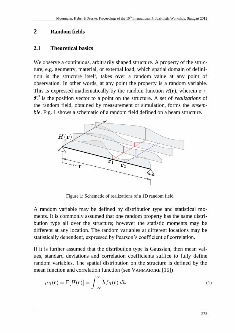
Moormann, Huber & Proske: Proceedings of the 10th International Probabilistic Workshop, Stuttgart 2012
273
2 Random fields
2.1 Theoretical basics
We observe a continuous, arbitrarily shaped structure. A property of the struc-
ture, e.g. geometry, material, or external load, which spatial domain of defini-
tion is the structure itself, takes over a random value at any point of
observation. In other words, at any point the property is a random variable.
This is expressed mathematically by the random function H(r), wherein r 3 is the position vector to a point on the structure. A set of realizations of
the random field, obtained by measurement or simulation, forms the ensem-
ble. Fig. 1 shows a schematic of a random field defined on a beam structure.
Figure 1: Schematic of realizations of a 1D random field.
A random variable may be defined by distribution type and statistical mo-
ments. It is commonly assumed that one random property has the same distri-
bution type all over the structure; however the statistic moments may be
different at any location. The random variables at different locations may be
statistically dependent, expressed by Pearson’s coefficient of correlation.
If it is further assumed that the distribution type is Gaussian, then mean val-
ues, standard deviations and correlation coefficients suffice to fully define
random variables. The spatial distribution on the structure is defined by the
mean function and correlation function (see VANMARCKE [15])
(1)

Bayer: Random Field Methods in Robustness Analysis
274
(2)
The latter is not equivalent to Pearson’s coefficient of correlation. This can be
derived from the correlation function by subtracting the mean values at r1, r2
and dividing by the respective standard deviations.
Two special cases shall be mentioned here:
2.1.1 Homogeneous random field
A homogeneous random field is characterized by constant moments through-
out the structure. It is comparable to a stationary random process. If this holds
for the functions of mean values and standard deviations only,
(3)
and if also the correlation function is independent of the reference location
(but on the difference vector between each two locations),
(4)
then the random field is called weak sense homogeneous. Since a Gaussian
distribution is fully defined by second moment characteristics, the above defi-
nitions will fulfil also strict homogeneity in the Gaussian case.
2.1.2 Isotropic random field
A random field is called weak sense homogeneous and isotropic, if the corre-
lation function is independent also from the relative position of each pair of
observed locations, but still depends on the absolute distance:
(5)
For simulation of an artificial, homogeneous isotropic random field one de-
fines a (one–dimensional) correlation coefficient function over the distance
(|| ||). This function must be positive definite. The -value of the centre of
gravity of the area beneath the function is a typical characteristic called corre-
lation length.
Moormann, Huber & Proske: Proceedings of the 10th International Probabilistic Workshop, Stuttgart 2012
275
2.2 Discretization
For any application in the context of computer aided engineering (CAE), the
continuous functions which define the random field have to be discretized.
Since the observed structure is given in discretized form by CAE methods
(FEM, CFD, etc.), it is instrumental to choose the same mesh for random field
discretization. Geometry random fields (manufacturing tolerances) are mod-
elled as shifts of node coordinates, element properties (such as e.g. material,
or residual strains), element mid points or integration points are chosen. How-
ever, if the random field is modelled based on measured data, usually the data
have to be transformed into the model coordinate system and mapped onto a
common reference mesh.
As result of discretization, one obtains a finite number n of random variables,
pooled in the random vector . The mean value function
becomes the mean vector . Variances and correla-
tions are given by the covariance matrix
(6)
The covariance matrix is, unlike typical finite element matrices, fully occu-
pied. Since each node or element of the structure is associated to a random
variable, the dimension of the covariance matrix becomes too high to be treat-
ed on the computer in a feasible way, with respect to both memory and com-
puting time for decomposition (see following section). In order to mitigate
this, a mesh coarsening algorithm has been proposed by BAYER [1] which
keeps the topology (relative refinement) of the original mesh. Data are
mapped from the original mesh to the random field discretization by local av-
eraging. For later post-processing on the original mesh, special interpolation
techniques are adapted from MOST et al. [9]. Although this is always a loss of
information, which is noted as a smoothing effect, it can be shown (as in
BAYER [3]) that in most cases the characteristics of the random field are re-
tained.
2.3 Spectral representation
As mentioned, the random variables which constitute a random field are usu-
ally correlated. An equivalent set of independent random variables (in the
weak sense) has to be found for two purposes. For the simulation of artificial
random fields, random number generators are able to handle independent var-
Bayer: Random Field Methods in Robustness Analysis
276
iables only. These have to be transformed to the physically meaningful, “real
world” variables. If the random field data are obtained e.g. by a manufactur-
ing process simulation, and the statistical relations between the input process
parameters and the resulting random fields shall be analyzed, then the decom-
position of the random field into independent components helps to isolate dif-
ferent effects and analyse correlations between the input and output side of
the process.
The random field shall be written as a Fourier-type series expansion, intro-
duced as Karhunen – Loève – series in PAPOULIS [13]:
(7)
The ortho-normal basic functions i in eq. (7) are determined as the eigen-
functions of the correlation function, eq. (2).
We observe the discrete, Gaussian, zero-mean random field, i.e. the mean
values may be subtracted before decomposition and if required, added to each
realization later again. Then the covariance matrix, cf. eq. (6), contains the
complete stochastic characterization of the random field. It can be shown, that
the basic functions in this case are the eigenvectors of the covariance matrix.
The eigenvalue analysis reads
(8)
In eq. (8), is the matrix of eigenvectors stored in columns. The coefficients
Yi in eq. (7) are also Gaussian distributed, zero-mean, and independent
(GHANEM et al. [8]. The standard deviations of the Yi are computed as the
square roots of the eigenvalues of CXX. Hence by
(9)
one defines a new set of random variables and obtains a series expansion of
the original random field X consisting of deterministic “shape functions”, i.e
the eigenvectors, and random, independent amplitudes Yi.
(10)
Moormann, Huber & Proske: Proceedings of the 10th International Probabilistic Workshop, Stuttgart 2012
277
If statistical data distributed on a structure are given (either by CAE simula-
tion or measurement), then with help of the inverse transformation of eq. (10)
it is possible to compute the corresponding sample of amplitudes.
(11)
The series expansion approach offers another opportunity for data reduction.
The eigenvalues are usually stored by the solver in a sorted manner, so it is
easy to choose those variables Yi which contribute most to the total scatter of
the random field. As experience from practical application, a drastic reduction
of the number of random variables is possible that way. This is always a nu-
merical advantage in simulation, but also helps to isolate the most relevant
effects in data analysis.
The truncation of the series expansion is nevertheless an approximation. A
measure of the approximation quality was introduced by BRENNER [5] as the
so-called variability fraction, defined as the ratio of the sum of variances of
the random variables considered to the total variance of the discrete random
field. When the dimensions of the original data grid and the random field dis-
cretization differ, then both numerator and denominator of this ratio must be
normalized to the respective number of points (BAYER et al. [4]).
(12)
3 Applications
3.1 Simulation of geometric tolerances
In the first application example, NUNES et al. [11] show the simulation of ge-
ometric tolerances of a car chassis part. The task was to examine the influence
of the random geometry on the dynamic behaviour and therefore on the ten-
dency of noise emission during brake.
Bayer: Random Field Methods in Robustness Analysis
278
From a 3D-scan we obtained the geometry of one real specimen as a triangu-
larized geometry in STL-format. The deviations of this measured geometry to
the finite element model were computed. The exact measure would be the dis-
tance normal to the surface through each point (node) of the reference model.
Since the number of measured points is far larger than the number of nodes,
the direct distance to the nearest neighbour, which is found by the approxi-
mate nearest neighbour (ANN) algorithm, is used instead.
One measurement was taken only; hence a statistical survey of an ensemble of
data sets at each node is not possible. Assuming ergodicity (VANMARCKE
[15]), the statistics pooling the values at all nodes into one sample were com-
puted. With a homogeneous variance obtained such and an assumed correla-
tion function (see sections 2.1.1 ff.), an artificial, but realistic random field for
geometric deviations was modelled.
Within a robustness analysis, Monte Carlo methods were applied to generate
samples of the random field parameters, create imperfect parts with random
geometry and put them into the CAE model of the entire chassis and brake
system. For each sampled structure, the brake squeal tendency was computed
with help of complex modal analysis.
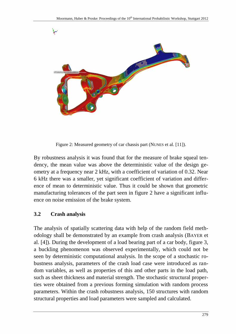
Moormann, Huber & Proske: Proceedings of the 10th International Probabilistic Workshop, Stuttgart 2012
279
Figure 2: Measured geometry of car chassis part (NUNES et al. [11]).
By robustness analysis it was found that for the measure of brake squeal ten-
dency, the mean value was above the deterministic value of the design ge-
ometry at a frequency near 2 kHz, with a coefficient of variation of 0.32. Near
6 kHz there was a smaller, yet significant coefficient of variation and differ-
ence of mean to deterministic value. Thus it could be shown that geometric
manufacturing tolerances of the part seen in figure 2 have a significant influ-
ence on noise emission of the brake system.
3.2 Crash analysis
The analysis of spatially scattering data with help of the random field meth-
odology shall be demonstrated by an example from crash analysis (BAYER et
al. [4]). During the development of a load bearing part of a car body, figure 3,
a buckling phenomenon was observed experimentally, which could not be
seen by deterministic computational analysis. In the scope of a stochastic ro-
bustness analysis, parameters of the crash load case were introduced as ran-
dom variables, as well as properties of this and other parts in the load path,
such as sheet thickness and material strength. The stochastic structural proper-
ties were obtained from a previous forming simulation with random process
parameters. Within the crash robustness analysis, 150 structures with random
structural properties and load parameters were sampled and calculated.

Bayer: Random Field Methods in Robustness Analysis
280
Figure 3: Standard deviations of plastic strain of a load bearing car part after crash robust-
ness analysis (BAYER et al. [4]).
The scatter of plastic strains which is plotted in figure 3 corresponds to the
observed buckling deformation. As it was explained in section 2.3, the spatial
scatter of the plastic strain was decomposed into “scatter shapes”; the respec-
tive samples of random amplitudes were computed following eq. (11). The
random amplitudes were statistically surveyed and related to the input random
variables.
Figure 4 shows the first three scatter shapes and their contributions to the total
scatter of plastic strain given in percent, cf. eq. (12). It is seen that with three
random amplitudes of the Karhunen – Loève – expansion only, in contrast to
ca. 5000 original variables (one for each finite element), it is possible to rep-
resent 98 % of total scatter. This demonstrates the efficiency of the random
field parametric proposed here.

Moormann, Huber & Proske: Proceedings of the 10th International Probabilistic Workshop, Stuttgart 2012
281
Figure 4: First three scatter shapes of plastic strain.
The algorithm Metamodel of Optimal Prognosis (MoP) of optiSLang (MOST
et al. [10]) was applied to relate the samples of the first three amplitudes to
the random parameters of the crash analysis. This algorithm uses the samples
of input – output sets as supports and fits a powerful interpolation model. As
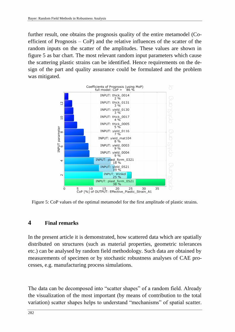
Bayer: Random Field Methods in Robustness Analysis
282
further result, one obtains the prognosis quality of the entire metamodel (Co-
efficient of Prognosis – CoP) and the relative influences of the scatter of the
random inputs on the scatter of the amplitudes. These values are shown in
figure 5 as bar chart. The most relevant random input parameters which cause
the scattering plastic strains can be identified. Hence requirements on the de-
sign of the part and quality assurance could be formulated and the problem
was mitigated.
Figure 5: CoP values of the optimal metamodel for the first amplitude of plastic strains.
4 Final remarks
In the present article it is demonstrated, how scattered data which are spatially
distributed on structures (such as material properties, geometric tolerances
etc.) can be analysed by random field methodology. Such data are obtained by
measurements of specimen or by stochastic robustness analyses of CAE pro-
cesses, e.g. manufacturing process simulations.
The data can be decomposed into “scatter shapes” of a random field. Already
the visualization of the most important (by means of contribution to the total
variation) scatter shapes helps to understand “mechanisms” of spatial scatter.
Moormann, Huber & Proske: Proceedings of the 10th International Probabilistic Workshop, Stuttgart 2012
283
By further statistical analysis of the respective amplitudes and their relation to
the random inputs, expressed as correlations, coefficients of determination of
a regression model or coefficients of prognosis of a MoP, the cause of scatter
can be identified.
It is also possible to model and sample random fields on the basis of empirical
data and/or model assumptions. With these artificial random fields, structural
parts with random properties are generated and fed into a CAE analysis. In
that way it is possible to study the sensitivity of a structure towards spatially
distributed random properties or loads.
Dynardo offers the software SoS (Statistics on Structure) for the analysis of
spatially scattering data. Statistical characteristics of the data can be plotted
on the structure, as well as the scatter shapes of the decomposed random field.
Samples of the respective random amplitudes can be exported as optiSLang
result file for further statistical analyses, in particular the relations to input
parameters, as it was demonstrated in the example of section 3.2.
5 Literature
[1] Bayer, V.; Roos, D.: Efficient Modelling and Simulation of Random Fields. 6th In-
ternational Probabilistic Workshop, Darmstadt 2008.
[2] Bayer, V.: Random Fields in Statistics on Structure. Weimar Optimization and Sto-
chastic Days 7.0, Weimar 2010.
[3] Bayer, V.: Random Fields – Applications in Robustness Analysis. Weimar Optimiza-
tion and Stochastic Days 8.0, Weimar 2011.
[4] Bayer, V.; Will, J.: Zufallsfelder in der Robustheits- und Zuverlässigkeitsbeurteilung
von Bauteilen. SIMVEC 2010 – Berechnung und Simulation im Fahrzeugbau. VDI,
Baden-Baden 2010.
[5] Brenner, C.E.: Ein Beitrag zur Zuverlässigkeitsanalyse von Strukturen unter Berück-
sichtigung von Systemuntersuchungen mit Hilfe der Methode der Stochastischen Fi-
nite Elemente. Dissertation, Leopold Franzens Universität Innsbruck 1995
[6] Bucher, C.: Basic concepts for robustness evaluation using stochastic analysis.
EUROMECH Colloq. Efficient Methods of Robust Design and Optimization, London
2007
[7] Bucher, C.: Computational Analysis of Randomness in Structural Mechanics. Taylor
& Francis, London 2009

Bayer: Random Field Methods in Robustness Analysis
284
[8] Ghanem, R.; Spanos, P.D.: Stochastic Finite Elements – a Spectral Approach.
Springer, New York, Berlin 1991
[9] Most, T.; Bucher, C.: A moving least square weighting function for the elementfree
galerkin method which almost fulfills essential boundary conditions. Structural En-
gineering and Mechanics 21, 2005
[10] Most, T.; Will, J.: Metamodel of optimized prognosis (MoP) - an automatic approach
for user friendly parameter optimization. Weimar Optimization and Stochastic Days
6.0, Weimar, 2009
[11] Nunes, R.; Will, J; Bayer, V.; Chittepu, K.: Robustness Evaluation of brake systems
concerned to squeal noise problem. Weimar Optimization and Stochastic Days 6.0,
Weimar 2009.
[12] Dynardo GmbH: optiSLang – the Optimizing Structural Language, User’s Manual
Version 3.1. Weimar 2009
[13] Papoulis, A.: Probability, Random Variables, and Stochastic Processes. McGraw–
Hill, New York 1991
[14] Dynardo GmbH: SoS – Statistics on Structure, User’s Manual Version 2.3.5., Wei-
mar 2011
[15] Vanmarcke, E.: Random Fields: Analysis and Synthesis. MIT Press, Cambridge,
USA, 1983
[16] Will, J.: State of the art - robustness in CAE-based virtual prototyping processes of
automotive applications. Weimar Optimization and Stochastic Days 4.0, Weimar
2007
Moormann, Huber & Proske: Proceedings of the 10th International Probabilistic Workshop, Stuttgart 2012
285
Probabilistic Assessment of Concrete Creep
Models under Repeated Loading Considering
Measurement Uncertainty
Hem Bahadur Motraa, Andrea Dimmig-Osburg
b and Joerg Hildebrand
c
aGraduiertenkolleg 1462, Bauhaus-Universität, Weimar Germany
bDepartment of Polymer Binder and Building Materials, Bauhaus-Universität
Weimar, Germany cDepartment of Simulation and Experiment, Bauhaus-Universität, Weimar,
Germany
Abstract: The aim of this paper is to present the analysis of the in-
fluence of some input variables on the creep deformation in concrete
for various models, namely BP model, Whaley and Neville model,
modified MC90 for cyclic loading and modified Hyperbolic function
for cyclic loading. Creep causes increased deflection in concrete struc-
tures and changes the stress distribution with in elements. The benefits
of an accurate prediction model of creep yields a safer design: a struc-
ture with minimum cracking, extended life and durability. The error in
determining the input variables and model itself can produce signifi-
cant changes in creep prediction values. The variability influence of
input random variables on the cyclic creep was studied by means of
the stochastic uncertainty and sensitivity analysis method. All input
parameters were considered to be random variables. The Latin Hyper-
cube Sampling (LHS) numerical simulation method (Monte Carlo
type method) was used. It has been found by the stochastic sensitivity
analysis that the cyclic creep deformation variability is most sensitive
to the Elastic modulus of concrete, compressive strength, mean stress,
cyclic stress amplitude, number of cycles, in that order. Further, it is
observed that the uncertainties of the creep prediction for all models
are compared and reveal significant differences. Due to the considera-
tion of three types of uncertainty which are included in uncertainty
quantification: (i) natural variability in loading materials properties;
(ii) data uncertainty due to measurement errors; and (iii) modelling
Motra, Osburg & Hildebrand: Probabilistic Assessment of Concrete Creep Models under Repeated Loading
286
uncertainty and errors during cyclic creep analysis, a measure for the
total variation of the model response is achieved. The study finds that
the BP, modified Hyperbolic and modified MC90 are the best per-
forming models for cyclic creep prediction - in that order.
1. Introduction
It is a well-known fact that the repeated loading of concrete causes irreversible
deformations GAEDE [8] and KERN et al. [13] called cyclic creep. The experi-
mental knowledge of this phenomenon is still rather limited but yet quite suffi-
cient for numerical prediction. When the principle of superposition is used to
estimate cyclic creep, the creep under cyclic loading of many repetitions is sig-
nificantly under-estimated. The reason behind this problem is that, the cyclic
creep is a non-linear phenomenon and principle of superposition is no longer
valid BAŽANT [1] and GVOZDEV [9]. The micro pre-stress solidification theory,
mechanical deformation theory, the viscous flow theory, the plastic flow theory,
the seepage of gel theory and the micro cracking theory can be explained by the
unidirectional non-linear creep under dynamic loading, which is proposed by
BAWEJA et al. [4], WHALEY et al. [24] and SUTER et al. [19]. This study can be
of importance for structures such as bridges carrying high traffic loads, struc-
tures carrying heavy vibrating machinery, ocean oil platform and other such
complex structures.
Creep and shrinkage are the most uncertain mechanical properties of concrete.
The stochastic aspects of these physical phenomena should therefore taken into
account in structural analysis and design. Structural responses have thus far been
treated as deterministic values in this study, although it was acknowledged that
the prediction models are marked with a certain degree of statistical variation.
Material and environmental parameters were also taken into account with their
expected mean value, but in reality they are also subjected to statistical variation
and prediction errors. Moreover, civil engineering constructions are naturally
subjected to variability; from many origins: their dimensions, their construction
processes, and their exposure to several loadings. Among these variables, which
influence the behaviour of a structure and; thus, its lifespan, some introduce a
variability on the material characteristics, evolving with time and are not neces-
sarily homogeneous in the whole structure, whereas some others create a varia-
bility on the loading itself, which the structure is subjected to.
Moormann, Huber & Proske: Proceedings of the 10th International Probabilistic Workshop, Stuttgart 2012
287
For all these aforementioned reasons, modelling the input parameter in a proba-
bilistic context makes sense SUDRET [18]. The uncertainty that affects the input
parameter may be of various kinds. They are usually classified as follows:
Aleatoric uncertainty: is an inherent variation associated with the physi-
cal or natural variability in the phenomenon under consideration. As an
examples, the number-of-cycles-to-failure of a samples specimen subject-
ed to fatigue loading shows aleatoric uncertainty, since the very life time
of the specimens of the same materials subjected to the same experimental
conditions varies one to the other SUDRET [18].
Epistemic uncertainty: is an uncertainty that is due to a lack of knowledge
of quantities or processes of the system and is also referred to as subjec-
tive uncertainty, reducible uncertainty, and model from uncertainty. As an
example, the lack of experimental data to characterize new materials and
processes, poor understanding of coupled physics phenomena. Further,
the compressive strength of concrete of a given shows scattering.
For the quantification of measurement uncertainties (as defined in the ISO/IEC
Guide 98-3 (2008a)) [11], namely the uncertainty based on a statistical analysis of
observations and the uncertainty derived from a process equation physically de-
scribing the measurement process. Both types of measurement uncertainties are
utilized for the derivation of a posterior measurement uncertainty by Bayesian
updating. This facilitates the quantification of a measurement uncertainty using
all available data of the measurement process. The measurement uncertainty
models derived are analysed through a sensitivity study and are discussed in de-
tail resulting in an identification of the most relevant sources of measurement
uncertainties THOENS [21].
Sensitivity Analysis (SA) techniques will perform better for specific type of
models. Sampling based methods are examined to scatter plots given by
HELTON [10]. One method of importance in the measurement of models by con-
sidering the uncorrelated and correlated parameters is proposed by XU et al.
[23]. The distinction between uncorrelated and correlated contribution of uncer-
tainty for an individual variable is very important and output response and the
input variables is approximately linear in this method. Method XU et al. [23] is
used in this present work.

Motra, Osburg & Hildebrand: Probabilistic Assessment of Concrete Creep Models under Repeated Loading
288
2. Cyclic creep models
Several experimental and mathematical models have been developed for esti-
mating cyclic creep strain. The most widely used mathematical models are the
BP [2] models, NEVIELLY [24] model. Modified MC90/EC2 [5] and modified
Hyperbolic function [17], experimental cyclic creep models: GAEDE [8], KERN
et al. [13], NEVILLE et al. [24], SUTER et al. [19]. This study also includes these
four mathematical models.
Based on the test data, Whaley and Neville models have shown that the cyclic
creep strain can be expressed as the sum of the two strain component, a mean
strain component and a cyclic strain component. We consider uniaxial stress de-
scribed as:
0
1sin(2 )
2t (1)
Where mean stress; ½Δ= cyclic stress amplitude; and circular frequen-
cy. The mean strain component is the creep strain produced by the static mean
stress (σm)=(σmax - σmin)/2. The additional cyclic creep component was found to
dependent on both mean stress (σm) and the stress range (Δ)= (σmax - σmin). They
proposed the following predictive equation for the total cyclic creep strain:
1
630( ) 129 (1 3.87 ) *10mt t t (2)
0
0 0 0
0
1 1el
c
t tt t t t t
E t (3)
Where ε (t - t0) is the cyclic creep strain, σm is the mean stress expressed as a
fraction of the compressive strength; and Δ is the stress-range expressed as a
fraction of the compressive strength and Φ (t - t0) is the creep function.
The above-noted static and dynamic components of dynamic creep are a func-
tion of time. It can be expressed as a function of a number of cycles also.
1 1
3 30 0 0( ) 129 17.8t t t N (4)
BP model takes into consideration both shrinkage strain and mechanical strain.
According to the BP model, cyclic creep function (t –t0)= ε/σmean , where ε is the
strain mean level of cycle, is as follows:
Moormann, Huber & Proske: Proceedings of the 10th International Probabilistic Workshop, Stuttgart 2012
289
0 0
1( ) ( ) ( ) ( )oc oc d d p o dt t C t t C t t t g C t t t f
E (5)
Where,
21
0 0 0
0
( ) ( )(1 ( )m n n
oc ppC t t t k t tE
(6)
and this equation modified:
' ' '
0 1 0 0 , 0( , , ) ( ) ( , ( , , ) ( , )c d dc p dct t q F C t t C t t t C t t t (7)
In which tdc can be calculated as:
1
' ' 2 34max( ) 1 10dct t t t F (8)
Here ω is the frequency (Hz), kω is the empirical constant and the function
F(σmax) is the nonlinearity over proportionality factors.
The long-time material model presented in the 1990 CEB Model Code MC90
[5] was chosen as the model. Static creep tests within the previously mentioned
and the modified by TERJE et al. [20] cyclic creep function is defined as:
0 00
1 ( ) ( )( )
( ) (28 ) (28 )
c cc
c o c c
t t t tt t
E t E d E d (9)
In these expression φc (t - to) is the static creep ratio and φcc is the cyclic creep
ratio, t’ the concrete age at loading and t the actual time. The cyclic creep ratio is
defined as:
0 0( ) ( ) ( ) ( ) ( ) ( , )cc cm m cct t t f S N (10)
In this expression cmf is the average compressive cylinder strength at 28 days;
mS the ratio between the mean stress and the concrete strength at the start of
testing; Δ the relative stress amplitude; N is the number of load cycles and ω is
the frequency 0( )N t t
0( , ) 1 (( )86400 ) 1, , 0.022n nN N t t with n (11)
The general expression for cyclic creep term is then written as:
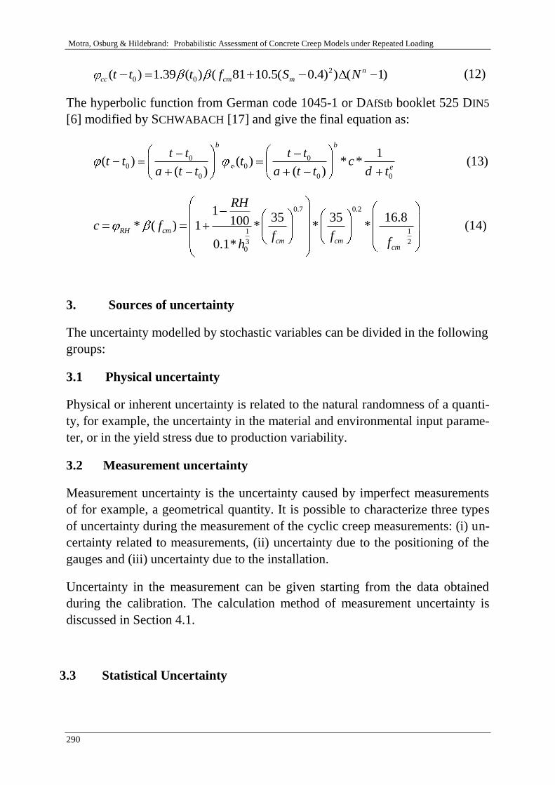
Motra, Osburg & Hildebrand: Probabilistic Assessment of Concrete Creep Models under Repeated Loading
290
2
0 0( ) 1.39 ( ) ( 81 10.5( 0.4) ) ( 1)n
cc cm mt t t f S N (12)
The hyperbolic function from German code 1045-1 or DAfStb booklet 525 DIN5
[6] modified by SCHWABACH [17] and give the final equation as:
0 00 0
0 0 0
1( ) ( ) * *
( ) ( )
b b
e
t t t tt t t c
a t t a t t d t (13)
0.7 0.2
1 1
3 20
135 35 16.8100* ( ) 1 * * *
0.1*
RH cm
cm cmcm
RH
c ff f
fh
(14)
3. Sources of uncertainty
The uncertainty modelled by stochastic variables can be divided in the following
groups:
3.1 Physical uncertainty
Physical or inherent uncertainty is related to the natural randomness of a quanti-
ty, for example, the uncertainty in the material and environmental input parame-
ter, or in the yield stress due to production variability.
3.2 Measurement uncertainty
Measurement uncertainty is the uncertainty caused by imperfect measurements
of for example, a geometrical quantity. It is possible to characterize three types
of uncertainty during the measurement of the cyclic creep measurements: (i) un-
certainty related to measurements, (ii) uncertainty due to the positioning of the
gauges and (iii) uncertainty due to the installation.
Uncertainty in the measurement can be given starting from the data obtained
during the calibration. The calculation method of measurement uncertainty is
discussed in Section 4.1.
3.3 Statistical Uncertainty

Moormann, Huber & Proske: Proceedings of the 10th International Probabilistic Workshop, Stuttgart 2012
291
Statistical uncertainty is due to limited sample sizes of observed quantities. A
stochastic quantity has one more property: a probability (density) distibution.
When doing a finite set of measurements, one can construct a histogram from
those measurements.
E(x)
Figure 1. Few observation… more observation theoretical limit
It should be noted that when the number of measurements increases, the histo-
gram will become more and more detailed, and in the limit become a smooth
function. This theoretical limit is called the stochastic quantity probability densi-
ty distribution function, distribution function for short. The Figure 1 shows the
quantity of observation and limit of expectation is a histogram.
3.4 Model Uncertainty
Model uncertainty is the uncertainty related to imperfect knowledge or idealiza-
tions of the mathematical models used or uncertainty related to the choice of
probability distribution types for the stochastic variables. Even when there oc-
curs no measurement uncertainty (or when it is negligible), there may be some
discrepancies between the predicted and observed values in most situations. This
is called model error or uncertainty.
4. Uncertainty quantification in measurement
4.1 Measurement uncertainty using Bayes method
The experimental results may be assessed using strategies based on conditional
probability concepts. These concepts are founded on Bayes’ theorem, which is
introduced by Thomas Bayes.
( ). ( )
( )[ ( ). ( )]
j
j
i i
P A B P BP B A
P A B P B (15)
Where,
Bj is a state of the unknown quantity
-σ +σ
● ●
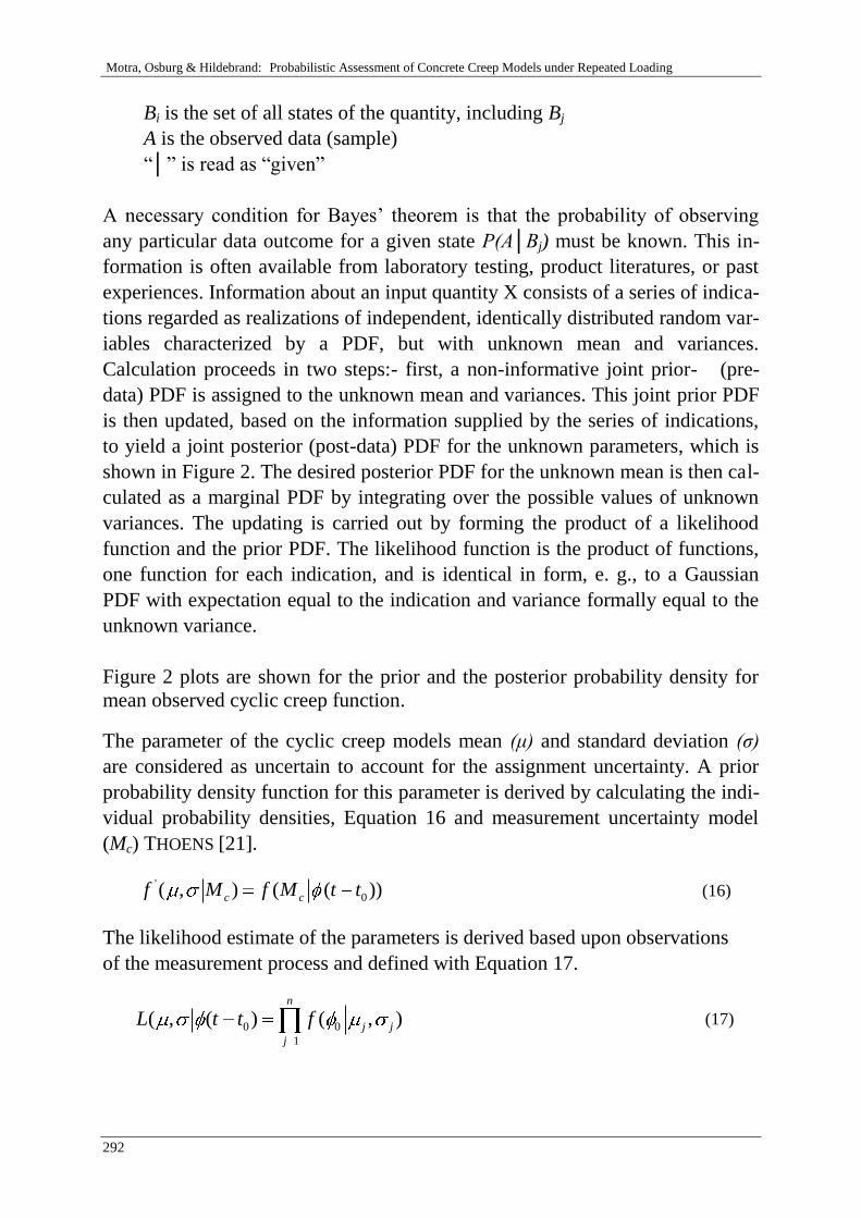
Motra, Osburg & Hildebrand: Probabilistic Assessment of Concrete Creep Models under Repeated Loading
292
Bi is the set of all states of the quantity, including Bj
A is the observed data (sample)
“│” is read as “given”
A necessary condition for Bayes’ theorem is that the probability of observing
any particular data outcome for a given state P(A│Bj) must be known. This in-
formation is often available from laboratory testing, product literatures, or past
experiences. Information about an input quantity X consists of a series of indica-
tions regarded as realizations of independent, identically distributed random var-
iables characterized by a PDF, but with unknown mean and variances.
Calculation proceeds in two steps:- first, a non-informative joint prior- (pre-
data) PDF is assigned to the unknown mean and variances. This joint prior PDF
is then updated, based on the information supplied by the series of indications,
to yield a joint posterior (post-data) PDF for the unknown parameters, which is
shown in Figure 2. The desired posterior PDF for the unknown mean is then cal-
culated as a marginal PDF by integrating over the possible values of unknown
variances. The updating is carried out by forming the product of a likelihood
function and the prior PDF. The likelihood function is the product of functions,
one function for each indication, and is identical in form, e. g., to a Gaussian
PDF with expectation equal to the indication and variance formally equal to the
unknown variance.
Figure 2 plots are shown for the prior and the posterior probability density for
mean observed cyclic creep function.
The parameter of the cyclic creep models mean (μ) and standard deviation (σ)
are considered as uncertain to account for the assignment uncertainty. A prior
probability density function for this parameter is derived by calculating the indi-
vidual probability densities, Equation 16 and measurement uncertainty model
(Mc) THOENS [21].
'
0( , ) ( ( ))c cf M f M t t (16)
The likelihood estimate of the parameters is derived based upon observations
of the measurement process and defined with Equation 17.
0 0
1
( , ( ) ( , )n
j j
j
L t t f (17)
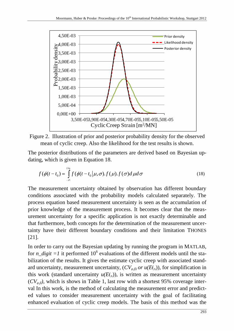
Moormann, Huber & Proske: Proceedings of the 10th International Probabilistic Workshop, Stuttgart 2012
293
Figure 2. Illustration of prior and posterior probability density for the observed
mean of cyclic creep. Also the likelihood for the test results is shown.
The posterior distributions of the parameters are derived based on Bayesian up-
dating, which is given in Equation 18.
0 0( ( ) ( ( , ). ( ). ( )f t t f t t f f d d (18)
The measurement uncertainty obtained by observation has different boundary
conditions associated with the probability models calculated separately. The
process equation based measurement uncertainty is seen as the accumulation of
prior knowledge of the measurement process. It becomes clear that the meas-
urement uncertainty for a specific application is not exactly determinable and
that furthermore, both concepts for the determination of the measurement uncer-
tainty have their different boundary conditions and their limitation THONES
[21].
In order to carry out the Bayesian updating by running the program in MATLAB,
for n_digit =1 it performed 106 evaluations of the different models until the sta-
bilization of the results. It gives the estimate cyclic creep with associated stand-
ard uncertainty, measurement uncertainty, (CVφ,β) or u(E )), for simplification in
this work (standard uncertainty u(E )), is written as measurement uncertainty
(CVφ,β), which is shows in Table 1, last row with a shortest 95% coverage inter-
val In this work, is the method of calculating the measurement error and predict-
ed values to consider measurement uncertainty with the goal of facilitating
enhanced evaluation of cyclic creep models. The basis of this method was the
0,00E+00
5,00E-04
1,00E-03
1,50E-03
2,00E-03
2,50E-03
3,00E-03
3,50E-03
4,00E-03
4,50E-03
3,50E-053,90E-054,30E-054,70E-055,10E-055,50E-05
Prior density
Likelihood density
Posterior density
Cyclic Creep Strain [m2/MN]
Pro
babil
ity d
ensi
ty
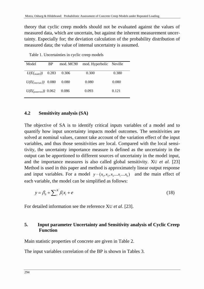
Motra, Osburg & Hildebrand: Probabilistic Assessment of Concrete Creep Models under Repeated Loading
294
theory that cyclic creep models should not be evaluated against the values of
measured data, which are uncertain, but against the inherent measurement uncer-
tainty. Especially for; the deviation calculation of the probability distribution of
measured data; the value of internal uncertainty is assumed.
Table 1. Uncertainties in cyclic creep models
Model BP mod. MC90 mod. Hyperbolic Neville
U(E(model)) 0.283 0.306 0.300 0.380
U(E(internal.)) 0.080 0.080 0.080 0.080
U(E(posterior)) 0.062 0.086 0.093 0.121
4.2 Sensitivity analysis (SA)
The objective of SA is to identify critical inputs variables of a model and to
quantify how input uncertainty impacts model outcomes. The sensitivities are
solved at nominal values, cannot take account of the variation effect of the input
variables, and thus those sensitivities are local. Compared with the local sensi-
tivity, the uncertainty importance measure is defined as the uncertainty in the
output can be apportioned to different sources of uncertainty in the model input,
and the importance measures is also called global sensitivity. XU et al. [23]
Method is used in this paper and method is approximately linear output response
and input variables. For a model 1 2 3( , , .... .... )i ky x x x x x and the main effect of
each variable, the model can be simplified as follows:
0
K
i iiy x e (18)
For detailed information see the reference XU et al. [23].
5. Input parameter Uncertainty and Sensitivity analysis of Cyclic Creep
Function
Main statistic properties of concrete are given in Table 2.
The input variables correlation of the BP is shown in Tables 3.
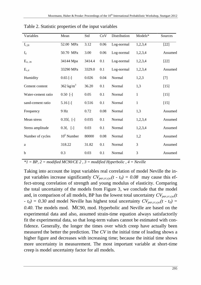
Moormann, Huber & Proske: Proceedings of the 10th International Probabilistic Workshop, Stuttgart 2012
295
Table 2. Statistic properties of the input variables
Variables Mean Std CoV Distribution Models* Sources
fc,28 52.00 MPa 3.12 0.06 Log-normal 1,2,3,4 [22]
fd 50.70 MPa 3.00 0.06 Log-normal 1,2,3,4 Assumed
Eci, 28 34144 Mpa 3414.4 0.1 Log-normal 1,2,3,4 [22]
Ec,d 33290 MPa 3329.0 0.1 Log-normal 1,2,3,4 Assumed
Humidity 0.65 [-] 0.026 0.04 Normal 1,2,3 [7]
Cement content 362 kg/m3 36.20 0.1 Normal 1,3 [15]
Water-cement ratio 0.50 [-] 0.05 0.1 Normal 1 [15]
sand-cement ratio 5.16 [-] 0.516 0.1 Normal 1 [15]
Frequency 9 Hz 0.72 0.08 Normal 1,3 Assumed
Mean stress 0.35fc [-] 0.035 0.1 Normal 1,2,3,4 Assumed
Stress amplitude 0.3fc [-] 0.03 0.1 Normal 1,2,3,4 Assumed
Number of cycles 106 Number 80000 0.08 Normal 1,2 Assumed
a 318.22 31.82 0.1 Normal 3 Assumed
b 0.3 0.03 0.1 Normal 3 Assumed
*1 = BP, 2 = modified MC90/CE 2 , 3 = modified Hyperbolic , 4 = Neville
Taking into account the input variables real correlation of model Neville the in-
put variables increase significantly CVpar,cr,cyc(t - t0) = 0.08 may cause this ef-
fect-strong correlation of strength and young modulus of elasticity. Comparing
the total uncertainty of the models from Figure 3, we conclude that the model
and, in comparison of all models, BP has the lowest total uncertainty CVpar,cr,cyc(t
- t0) = 0.30 and model Neville has highest total uncertainty CVpar,cr,cyc(t - t0) =
0.40. The models mod. MC90, mod. Hyperbolic and Neville are based on the
experimental data and also, assumed strain-time equation always satisfactorily
fit the experimental data, so that long-term values cannot be estimated with con-
fidence. Generally, the longer the times over which creep have actually been
measured the better the prediction. The CV in the initial time of loading shows a
higher figure and decreases with increasing time; because the initial time shows
more uncertainty in measurement. The most important variable at short-time
creep is model uncertainty factor for all models.
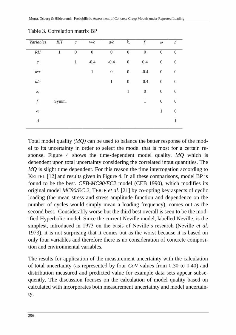
Motra, Osburg & Hildebrand: Probabilistic Assessment of Concrete Creep Models under Repeated Loading
296
Table 3. Correlation matrix BP
Total model quality (MQ) can be used to balance the better response of the mod-
el to its uncertainty in order to select the model that is most for a certain re-
sponse. Figure 4 shows the time-dependent model quality. MQ which is
dependent upon total uncertainty considering the correlated input quantities. The
MQ is slight time dependent. For this reason the time interrogation according to
KEITEL [12] and results given in Figure 4. In all these comparisons, model BP is
found to be the best. CEB-MC90/EC2 model (CEB 1990), which modifies its
original model MC90/EC 2, TERJE et al. [21] by co-opting key aspects of cyclic
loading (the mean stress and stress amplitude function and dependence on the
number of cycles would simply mean a loading frequency), comes out as the
second best. Considerably worse but the third best overall is seen to be the mod-
ified Hyperbolic model. Since the current Neville model, labelled Neville, is the
simplest, introduced in 1973 on the basis of Neville’s research (Neville et al.
1973), it is not surprising that it comes out as the worst because it is based on
only four variables and therefore there is no consideration of concrete composi-
tion and environmental variables.
The results for application of the measurement uncertainty with the calculation
of total uncertainty (as represented by four CoV values from 0.30 to 0.40) and
distribution measured and predicted value for example data sets appear subse-
quently. The discussion focuses on the calculation of model quality based on
calculated with incorporates both measurement uncertainty and model uncertain-
ty.
Variables RH c w/c a/c ks fc ω Δ
RH 1 0 0 0 0 0 0 0
c 1 -0.4 -0.4 0 0.4 0 0
w/c 1 0 0 -0.4 0 0
a/c 1 0 -0.4 0 0
ks 1 0 0 0
fc Symm. 1 0 0
ω 1 0
Δ 1
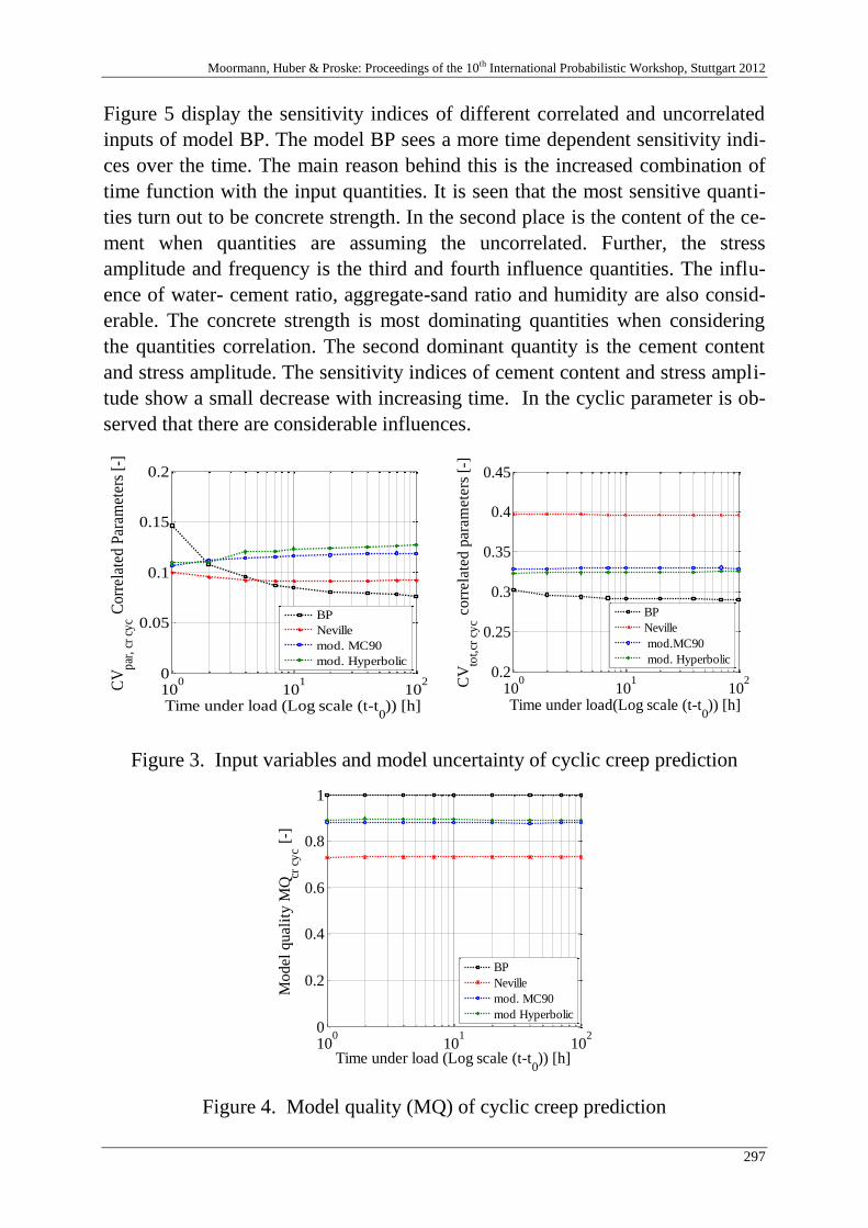
Moormann, Huber & Proske: Proceedings of the 10th International Probabilistic Workshop, Stuttgart 2012
297
Figure 5 display the sensitivity indices of different correlated and uncorrelated
inputs of model BP. The model BP sees a more time dependent sensitivity indi-
ces over the time. The main reason behind this is the increased combination of
time function with the input quantities. It is seen that the most sensitive quanti-
ties turn out to be concrete strength. In the second place is the content of the ce-
ment when quantities are assuming the uncorrelated. Further, the stress
amplitude and frequency is the third and fourth influence quantities. The influ-
ence of water- cement ratio, aggregate-sand ratio and humidity are also consid-
erable. The concrete strength is most dominating quantities when considering
the quantities correlation. The second dominant quantity is the cement content
and stress amplitude. The sensitivity indices of cement content and stress ampli-
tude show a small decrease with increasing time. In the cyclic parameter is ob-
served that there are considerable influences.
100
101
102
0
0.05
0.1
0.15
0.2
Time under load (Log scale (t-t0)) [h]
CV
par
, cr
cy
c C
orre
late
d P
aram
eter
s [-
]
BP
Neville
mod. MC90
mod. Hyperbolic
100
101
102
0.2
0.25
0.3
0.35
0.4
0.45
Time under load(Log scale (t-t0)) [h]
CV
tot,
cr c
yc c
orr
ela
ted p
ara
mete
rs [
-]
BP
Neville
mod.MC90
mod. Hyperbolic
Figure 3. Input variables and model uncertainty of cyclic creep prediction
100
101
102
0
0.2
0.4
0.6
0.8
1
Time under load (Log scale (t-t0)) [h]
Model
quali
ty M
Qcr
cy
c [
-]
BP
Neville
mod. MC90
mod Hyperbolic
Figure 4. Model quality (MQ) of cyclic creep prediction
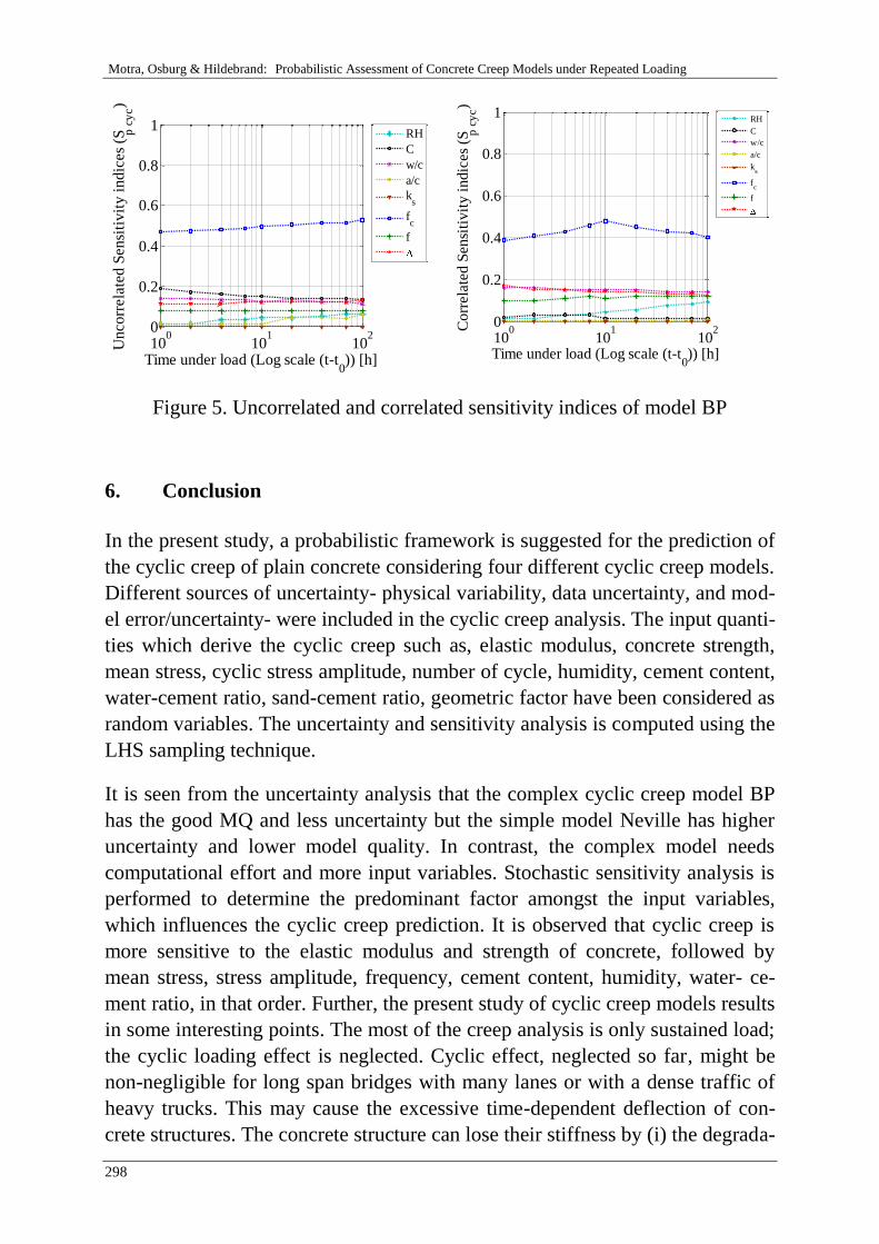
Motra, Osburg & Hildebrand: Probabilistic Assessment of Concrete Creep Models under Repeated Loading
298
100
101
102
0
0.2
0.4
0.6
0.8
1
Time under load (Log scale (t-t0)) [h]
Uncorr
ela
ted S
ensi
tivit
y i
ndic
es
(Sp
cy
c)
RH
C
w/c
a/c
ks
fc
f
100
101
102
0
0.2
0.4
0.6
0.8
1
Time under load (Log scale (t-t0)) [h]
Co
rrela
ted
Sen
siti
vit
y i
nd
ices
(Sp
cy
c)
RH
C
w/c
a/c
ks
fc
f
Figure 5. Uncorrelated and correlated sensitivity indices of model BP
6. Conclusion
In the present study, a probabilistic framework is suggested for the prediction of
the cyclic creep of plain concrete considering four different cyclic creep models.
Different sources of uncertainty- physical variability, data uncertainty, and mod-
el error/uncertainty- were included in the cyclic creep analysis. The input quanti-
ties which derive the cyclic creep such as, elastic modulus, concrete strength,
mean stress, cyclic stress amplitude, number of cycle, humidity, cement content,
water-cement ratio, sand-cement ratio, geometric factor have been considered as
random variables. The uncertainty and sensitivity analysis is computed using the
LHS sampling technique.
It is seen from the uncertainty analysis that the complex cyclic creep model BP
has the good MQ and less uncertainty but the simple model Neville has higher
uncertainty and lower model quality. In contrast, the complex model needs
computational effort and more input variables. Stochastic sensitivity analysis is
performed to determine the predominant factor amongst the input variables,
which influences the cyclic creep prediction. It is observed that cyclic creep is
more sensitive to the elastic modulus and strength of concrete, followed by
mean stress, stress amplitude, frequency, cement content, humidity, water- ce-
ment ratio, in that order. Further, the present study of cyclic creep models results
in some interesting points. The most of the creep analysis is only sustained load;
the cyclic loading effect is neglected. Cyclic effect, neglected so far, might be
non-negligible for long span bridges with many lanes or with a dense traffic of
heavy trucks. This may cause the excessive time-dependent deflection of con-
crete structures. The concrete structure can lose their stiffness by (i) the degrada-
Moormann, Huber & Proske: Proceedings of the 10th International Probabilistic Workshop, Stuttgart 2012
299
tion of concrete, (ii) the creep of concrete etc. The relation between the frequen-
cy of the structure and its age is important for the study of the long-term behav-
iour of materials, possibly for the detection of its damage. Of significance is the
change of the modulus of elasticity of concrete due to cyclic creep.
Also, the proposed approach for UQ and SA is applicable to several engineer-
ing disciplines and the domain of cyclic creep analysis was used only as an illus-
tration to develop the methodology. In general, the proposed methodology
provides a fundamental framework in which multiple models can be connected
through a Bayes network and the confidence in the overall model prediction can
be assessed quantitatively.
Acknowledgment
This research is supported by the German Research Institute (DFG) via Re-
search Training Group ”Evaluation of Coupled Numerical Partial Models in
Structural Engineering (GRK 1462)”, and is gratefully acknowledged by the au-
thors.
References
[1] Bažant, Z.P. : Creep of concrete in structural analysis, SNTL (State Publ. House of Techn
Lit.), Prague 1966
[2] Bažant, Z. P.; Panula, L.: Practical prediction of time-dependent deformation of concrete
(Part IV: Cyclic creep, nonlinearity and statistical scatter) J. Mat. Struct. 1979, 12 (69),
pp. 175-183
[3] Bažant, Z. P.; Kim, J. : Improved prediction model for time-dependent deformation of
concrete: (Part 5- Cyclic load and cyclic humidity), J. Mat. Struct. 1992, 25. pp 163-169
[4] Bazant , Z. P.; Hauggaaed A. B.; Baweja S.; Ulm F. J.: Microprestress-solidification theo-
ry for concrete creep. I: Aging and drying effects, Journal of Engineering Mechanics, vol.
123, 11, p. 1188-1194, 1997a
[5] CEB - Comite Euro-International du Beton: CEB-FIP Model Code 1990 / Comite Euro-
International du Beton. 1993. - Technical Report 43
[6] DIN: DAfStb Heft 525: Erläuterungen zur DIN 1045-1. Deutscher Ausschuss für Stahlbe-
ton DAfStb,1 Auflage, 2003, September

Motra, Osburg & Hildebrand: Probabilistic Assessment of Concrete Creep Models under Repeated Loading
300
[7] Diamantidis, D.; Madsen, H.; Rackwitz, R.: On the variability of the creep coefficient of
structural concrete. Mater Constr 1984, 17(100):321-8
[8] Gaede, K.: Über die Festigkeit und die Verformung von Beton bei Druck-
Schwellbeanspruchung. Deutscher Ausschuss für Stahlbeton, Heft 144, Berlin 1962, Ver-
trieb durch Verlag von Wilhelm Ernst und Sohn.
[9] Gvozdev, A. A. : Creep of concrete. In Mekhanika Tverdogo Tela (Conference Proc.)
Acad. Sci. USSR, Nauka Moscow 1966, pp. 137-152
[10] Helton, J. C.; Davis, F. J.: Latin hypercube sampling and the propagation of uncertainty
in analyses of complex systems. Reliability Engineering & System Safety 2003;81(1):23–
69.
[11] International Organization for Standardization, ISO/IEC Guide 98-3:2008 – Uncertainty
of Measurement - Part 3: Guide to the Expression of Uncertainty in Measurement
(GUM), ISO, 2008
[12] Keitel, H.: Evaluation Methods for the Prediction Quality of Creep Models of Concrete,
Bauhaus-Universität Weimar, Dissertation, 2011
[13] Kern, E.; Mehmel, A. : Elastische und Plastische Stauchungen von Beton infolge
Druckschwell-und Standbelastung, Deutsche. Ausschuss für Stahlbeton, Heft 153, W.
Ernst, Berlin 1962
[14] Li, G. H.; Bažant, Z. P.: Unbiased Statistical Comparison of Creep and Shrinkage Pre-
diction Models. In: ACI Materials Journal, 105(6) (2008)
[15] Madsen, H.; Bažant, Z.: Uncertainty analysis of creep and shrinkage effects in concrete
structures. ACI J B 1983; 80:116–27
[16] Mckay, M. D.; Beckman, R. J.; Conover, W. J.: Comparison of 3 Methods for Selecting
Values of Input Variables in the Analysis of Output from a Computer Code. Technomet-
rics 1979;21(2):239–245
[17] Schwabach, E.: Verformungs- und Degradationsverhalten von niederzyklisch uniaxial
druckbeanspruchtem Beton. Dissertation an der Fakultt Bauingenieurwesen der Bauhaus-
Universitt Weimar, 2005
[18] Sudret, B.: Uncertainty propagation and sensitive analysis in mechanical models and
contribution to structural reliability and stochastic spectral methods, Universite Blaise
Pascal, Clermont-Ferrand, 2007
[19] Suter, G.T.; Mickleborough, N. C. : Creep of concrete under cyclically varying dynamic
loads. Cement and Concrete Research, Vol. 5, No. 6, 1975. Pp.565-576
[20] Terje, K.; Gordana, P.: Material model for high strength concrete exposed to cyclic load-
ing , Fracture mechanics and concrete structures Edited by Z.P Bažant, 1992

Moormann, Huber & Proske: Proceedings of the 10th International Probabilistic Workshop, Stuttgart 2012
301
[21] Thoens, S.: Monitoring based Condition Assessment of Offshore Wind Turbine Support
Structures, Dissertation ETH Zurich, 2011
[22] Vrouwenvelder, T.: Probabilistic model code. 12th draft. Tech. rep. Joint Committee on
Structural Safety. 2002
[23] Xu, C.; Gertner, G. Z.: Uncertainty and Sensitivity Analysis for Models with Correlated
Parameters. In: Reliability Engineering and System Safety, 2008, 93 , S. 1563-1573 7,
61
[24] Whaley, C. P.; Neville, A. M. : Non-elastic deformation of concrete under cyclic com-
pression. Magazine of Concrete Research. Vol. 25, No. 84. September 1973 pp. 145-154

Motra, Osburg & Hildebrand: Probabilistic Assessment of Concrete Creep Models under Repeated Loading
302
Moormann, Huber & Proske: Proceedings of the 10th International Probabilistic Workshop, Stuttgart 2012
303
Fuzzy and statistical conformity criteria for
compressive strength according to EN 206-1
Izabela Skrzypczak
Institute of Geodesy, University of Technology, Rzeszow
Abstract: Statistical conformity criteria for compressive strength of concrete
for small sample size n=3 are matter of the debate. Statistical criteria can have
prejudicial effects to both - producer and client. In the code this is taken into
account by choosing of optional decision for the acceptance of batch of con-
crete. These ones are checked from the economical and statistical decision of
view. Statistical and fuzzy method of quality control, and especially compli-
ance criteria for concrete recommended in code EN 206-1 and fuzzy criteria
based on the fuzzy sets are presented and discussed.
1 Introduction
In order to achieve a sufficient level of the reliability required for a concrete
structure the strength distribution and parameters of concrete supplied to a
construction site should be in accordance with the assumptions specified in
the design. Thus in each lot of concrete the conformity of the compressive
strength should be verified using an adequate conformity criteria. Statistical
conformity criteria specified in different codes and standards [1, 2, 3] are usu-
ally compounded of two elements and can be expressed as follows:
1ck kfx and 2ckmin kfx (1)
where min, xx are the sample mean and minimum value of the compressive
strength of concrete, ckf is the characteristic value of the concrete compres-
sive strength specified by the producer, 21 ,kk are parameters that depend on
different circumstances, for example: nsk1 , )87.14.1( ; is the pa-
rameter that depends on the tolerance limit and the fractile considered, ns is
the sampling standard deviation, or )51(1k MPa and )51(2k MPa [5].
Skrzypczak: Fuzzy and statistical conformity criteria for compressive strength according to EN 206-1
304
In the European Standard EN 206-1 [1] the statistical compliance criteria for
compressive strength of concrete for continuous production are given as fol-
lows:
for n=3 of results in the group
4ff ckcm , 4ff ckci (2)
for n≥15 of results in the group
1,48σff ckcm , 4ff ckci 4ff ckci (3)
These criteria are far from perfection and there is always the risk that the suit-
able lot of concrete can be rejected (producer’s risk and loss) or that the defec-
tive lot can be accepted (contractor’s or/and investor’s risk).
Compound compliance criteria of type (2) raises many questions, so the anal-
ysis reference is made to the sample size n = 3 using the methods of statistical
and fuzzy. The paper presents an analysis and assessment of the quality and
safety associated with the use codes compliance criteria for compressive
strength of ordinary concrete of one kind. Method was used for analysis of
random Monte Carlo simulation and the theory of fuzzy numbers using fuzzy
statistical methods.
2 OC- curves (operating-characteristic curves)
Performance and efficiency of the statistical conformity criteria are investi-
gated using the operation characteristic curves (OC curves). The probability
of acceptance aP is calculated by means of numerical simulation using the
Monte Carlo technique and simulation programs.
The simulation programs for this purpose were elaborated for normal distribu-
tion with several known standard deviation, obtaining the operating character-
istic curves shown in Figures 2 and 3 for compressive strength criteria
specified in PN- EN 206-1. Similar procedure has been adopted by Taerwe
[7].
OC curves calculated of single criterion and compound criterion. Denote by:
A - the event. that 4ckn fx ,
B - the event. that 4fx ckmin
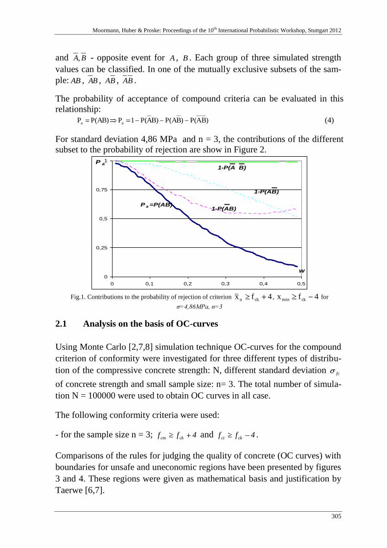
Moormann, Huber & Proske: Proceedings of the 10th International Probabilistic Workshop, Stuttgart 2012
305
and BA, - opposite event for A , B . Each group of three simulated strength
values can be classified. In one of the mutually exclusive subsets of the sam-
ple: AB , BA , BA , BA .
The probability of acceptance of compound criteria can be evaluated in this
relationship:
)BAP()BP(AB)AP(1PP(AB)P aa (4)
For standard deviation 4,86 MPa and n = 3, the contributions of the different
subset to the probability of rejection are show in Figure 2.
0
0,25
0,5
0,75
1
0 0,1 0,2 0,3 0,4 0,5
w
P a
P a =P(AB)
1-P(AB)
1-P(AB)
1-P(A B)
Fig.1. Contributions to the probability of rejection of criterion 4fx ckn , 4fx ckmin for
σ=4,86MPa, n=3
2.1 Analysis on the basis of OC-curves
Using Monte Carlo [2,7,8] simulation technique OC-curves for the compound
criterion of conformity were investigated for three different types of distribu-
tion of the compressive concrete strength: N, different standard deviation fc
of concrete strength and small sample size: n= 3. The total number of simula-
tion N = 100000 were used to obtain OC curves in all case.
The following conformity criteria were used:
- for the sample size n = 3; 4ff ckcm and 4ff ckci .
Comparisons of the rules for judging the quality of concrete (OC curves) with
boundaries for unsafe and uneconomic regions have been presented by figures
3 and 4. These regions were given as mathematical basis and justification by
Taerwe [6,7].

Skrzypczak: Fuzzy and statistical conformity criteria for compressive strength according to EN 206-1
306
Taerwe’s definition of the boundary of the unsafe region is:
500Pw a (5)
and of the uneconomic region is:
0,05P100
w
a
(6)
These boundaries are shown on Figure 2 as dashed lines.
If conformity rule gives an operating characteristic that passes through the
unsafe region than the protection it gives the specifier would be too weak. If
a rule gives an operating characteristic that passes through the uneconomic
region it causes producers to use excessively large margins, even then, accept
high risks of non-conformity [6].
OC curve for criteria (2) shown in Fig.3 to Fig.4 for samples n=3 for normal
(N) distributions with known standard deviation.
Prediction accuracy of statistical acceptance criteria has been determinate
with use of normal distribution. Taking the compliance compound criterion
into consideration, higher values of acceptance probability Pa correspond to
lots of bigger strength variability. The lower probability of acceptance has been for N
distributions of higher strength variability.
High values of probability of acceptance have been of productions with more
than 5% of defects, which can be around 80% in some cases. For standard
conformity criteria probability of acceptance of all is higher, the higher is
standard deviation of concrete compressive strength. It may lead to increasing
of mean concrete strength at growing spread causing groundless costs of a
producer. Conformity criterion of concrete compressive strength for small
sample size discourages from concrete production with small scatter.
selection of materials, concrete design and production, inspection and control,
test results. Only one type of restricted information connected with numerical
measurements, namely the values of standard deviation and minimum
strength are taken into consideration in the statistical conformity criteria. The
wide information on the composition, production, placing, curing and testing
of concrete is mostly qualitative, verbal, subjective and imprecise. Statistical
procedures ignore this type of data. Application of the fuzzy sets theory and
approximate reasoning scheme enables to take advantage of qualitative and
quantitative information, sharp and vague data for conformity assessment of
concrete strength.
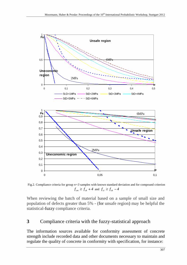
Moormann, Huber & Proske: Proceedings of the 10th International Probabilistic Workshop, Stuttgart 2012
307
0
0,5
1
0 0,1 0,2 0,3 0,4 0,5
w
Pa
St.D=1MPa StD=2MPa StD=3MPa StD=4MPa
StD=5MPa StD=6MPa
Unsafe region
Uneconomic
region2MPa
6MPa
0
0,1
0,2
0,3
0,4
0,5
0,6
0,7
0,8
0,9
1
0 0,05 0,1
w
Pa
Uneconomic region
Unsafe region
2MPa
6MPa
Fig.2. Compliance criteria for group n=3 samples with known standard deviation and for compound criterion
4ff ckcm and 4ff ckci
When reviewing the batch of material based on a sample of small size and
population of defects greater than 5% - (for unsafe region) may be helpful the
statistical-fuzzy compliance criteria.
3 Compliance criteria with the fuzzy-statistical approach
The information sources available for conformity assessment of concrete
strength include recorded data and other documents necessary to maintain and
regulate the quality of concrete in conformity with specification, for instance:
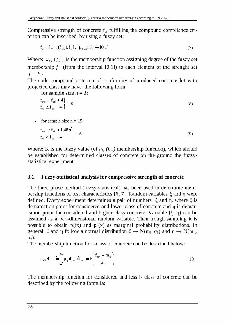
Skrzypczak: Fuzzy and statistical conformity criteria for compressive strength according to EN 206-1
308
Compressive strength of concrete fc, fulfilling the compound compliance cri-
terion can be inscribed by using a fuzzy set:
]f),(f[μf ccmC,fc , [0,1]F:μ cC,f (7)
Where: )(, cmCf f is the membership function assigning degree of the fuzzy set
membership fc (from the interval [0,1]) to each element of the strenght set
cc Ff .
The code compound criterion of conformity of produced concrete lot with
projected class may have the following form:
for sample size n = 3:
K4ff
4ff
ckci
ckcm (8)
for sample size n = 15:
K4ff
1,48σff
ckci
ckcm (9)
Where: K is the fuzzy value (of μfc (fcm) membership function), which should
be established for determined classes of concrete on the ground the fuzzy-
statistical experiment.
3.1. Fuzzy-statistical analysis for compressive strength of concrete
The three-phase method (fuzzy-statistical) has been used to determine mem-
bership functions of test characteristics [6, 7]. Random variables ξ and η were
defined. Every experiment determines a pair of numbers ξ and η, where ξ is
demarcation point for considered and lower class of concrete and η is demar-
cation point for considered and higher class concrete. Variable (ξ ,η) can be
assumed as a two-dimensional random variable. Then trough sampling it is
possible to obtain pξ(x) and pη(x) as marginal probability distributions. In
general, ξ and η follow a normal distribution ξ → N(mξ, σξ) and η → N(mη,,
ση).
The membership function for i-class of concrete can be described below:
η
ηcm
cm
f
cmηcmCiσ
mfFdffpfμ
cm
(10)
The membership function for considered and less i- class of concrete can be
described by the following formula:
Moormann, Huber & Proske: Proceedings of the 10th International Probabilistic Workshop, Stuttgart 2012
309
ξ
ξcm
cm
f
cmξcm1Ciσ
mfF1dffpfμ
cm
(11)
Contrast, the fuzzy membership functions considered and higher i- class of
concrete has follow form:
cm
cm
f
cmηcm
f
cmξcm1Ci ffpdffp1fμ (12)
η
ηcm
ξ
ξcm
cm1Ciσ
mfF
σ
mfF11fμ
(13)
The final form of the formula is:
η
ηcm
ξ
ξcm
cm1Ciσ
mfF
σ
mfFfμ (14)
Where:
)dz0,5zexp(2π
1F(z)
z
2 (15)
With the membership functions for different classes of concrete, and the mean
value of compressive strength for neighboring classes estimated based on ran-
dom simulation, we can calculate the degree of membership values of the
considered batch of concrete to different classes. Depending on the value of
)(, cmCif f , we can decide on the inclusion of lots of concrete to the appropriate
class of concrete. This decision may be more or less conservative, depending
on its impact on the qualitative assessment of the produced concrete and the
impact on the requirements of safety, quality and economics.
4. Examples with application of fuzzy-statistical method
Compliance criteria given in the formulas (1) were performed by the compu-
tations method: generating 100 000 random groups of size n=3 in accordance
with normal distribution, generating class of concrete (concrete classes of the
three neighboring classes of concrete Ci -1, Ci, Ci + 1 with 1/3 probability), gen-
erating standard deviation and defective fraction. To generate random num-
bers with standard normal distribution, the method Box and Muller [5] was
used. The table of probability distribution of random vector and the
histogram of marginal probability distributions, for the considered and lower
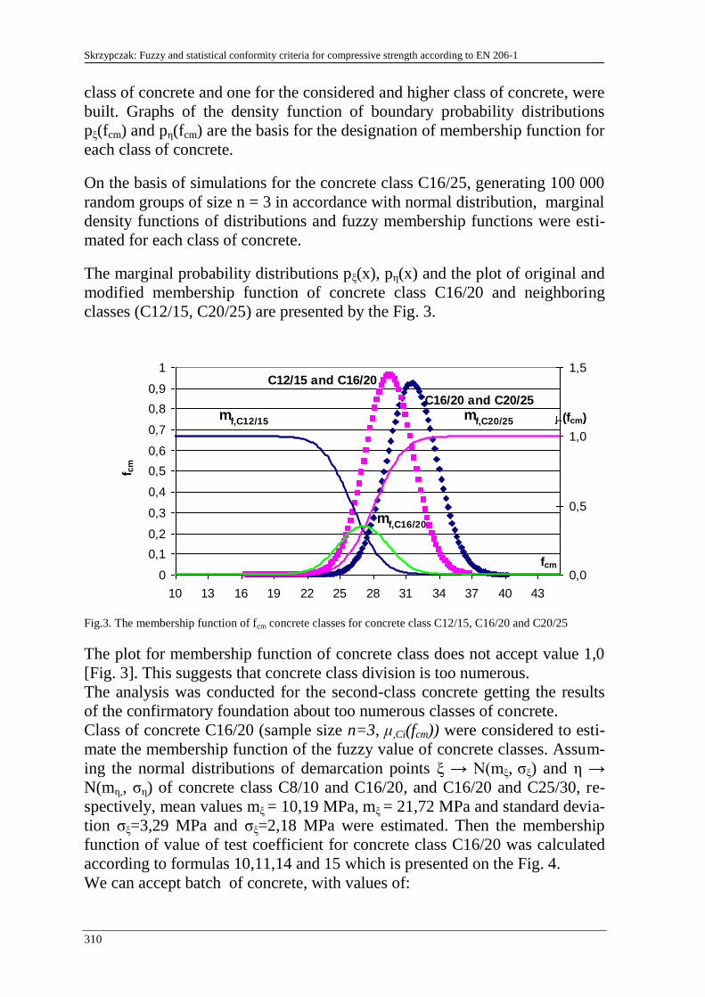
Skrzypczak: Fuzzy and statistical conformity criteria for compressive strength according to EN 206-1
310
class of concrete and one for the considered and higher class of concrete, were
built. Graphs of the density function of boundary probability distributions
pξ(fcm) and pη(fcm) are the basis for the designation of membership function for
each class of concrete.
On the basis of simulations for the concrete class C16/25, generating 100 000
random groups of size n = 3 in accordance with normal distribution, marginal
density functions of distributions and fuzzy membership functions were esti-
mated for each class of concrete.
The marginal probability distributions pξ(x), pη(x) and the plot of original and
modified membership function of concrete class C16/20 and neighboring
classes (C12/15, C20/25) are presented by the Fig. 3.
0
0,1
0,2
0,3
0,4
0,5
0,6
0,7
0,8
0,9
1
10 13 16 19 22 25 28 31 34 37 40 43
fcm
f
cm
0,0
0,5
1,0
1,5
(fcm)
C12/15 and C16/20
C16/20 and C20/25
mf,C16/20
mf,C20/25
mf,C12/15
Fig.3. The membership function of fcm concrete classes for concrete class C12/15, C16/20 and C20/25
The plot for membership function of concrete class does not accept value 1,0
[Fig. 3]. This suggests that concrete class division is too numerous.
The analysis was conducted for the second-class concrete getting the results
of the confirmatory foundation about too numerous classes of concrete.
Class of concrete C16/20 (sample size n=3, μ,Ci(fcm)) were considered to esti-
mate the membership function of the fuzzy value of concrete classes. Assum-
ing the normal distributions of demarcation points ξ → N(mξ, σξ) and η →
N(mη,, ση) of concrete class C8/10 and C16/20, and C16/20 and C25/30, re-
spectively, mean values mξ = 10,19 MPa, mξ = 21,72 MPa and standard devia-
tion σξ=3,29 MPa and σξ=2,18 MPa were estimated. Then the membership
function of value of test coefficient for concrete class C16/20 was calculated
according to formulas 10,11,14 and 15 which is presented on the Fig. 4.
We can accept batch of concrete, with values of:
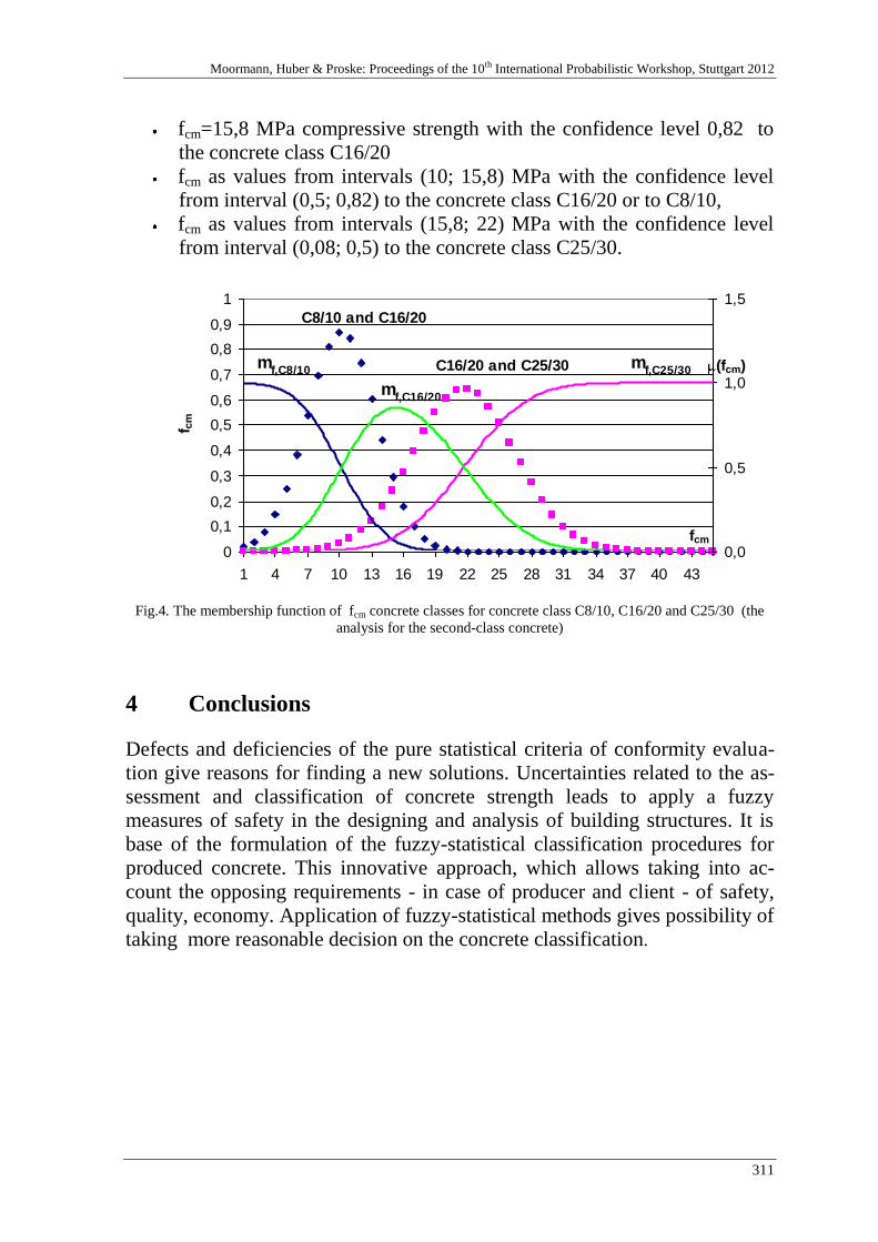
Moormann, Huber & Proske: Proceedings of the 10th International Probabilistic Workshop, Stuttgart 2012
311
fcm=15,8 MPa compressive strength with the confidence level 0,82 to
the concrete class C16/20
fcm as values from intervals (10; 15,8) MPa with the confidence level
from interval (0,5; 0,82) to the concrete class C16/20 or to C8/10,
fcm as values from intervals (15,8; 22) MPa with the confidence level
from interval (0,08; 0,5) to the concrete class C25/30.
0
0,1
0,2
0,3
0,4
0,5
0,6
0,7
0,8
0,9
1
1 4 7 10 13 16 19 22 25 28 31 34 37 40 43
fcm
f c
m
0,0
0,5
1,0
1,5
(fcm)
C8/10 and C16/20
C16/20 and C25/30
mf,C16/20
mf,C25/30
mf,C8/10
Fig.4. The membership function of fcm concrete classes for concrete class C8/10, C16/20 and C25/30 (the
analysis for the second-class concrete)
4 Conclusions
Defects and deficiencies of the pure statistical criteria of conformity evalua-
tion give reasons for finding a new solutions. Uncertainties related to the as-
sessment and classification of concrete strength leads to apply a fuzzy
measures of safety in the designing and analysis of building structures. It is
base of the formulation of the fuzzy-statistical classification procedures for
produced concrete. This innovative approach, which allows taking into ac-
count the opposing requirements - in case of producer and client - of safety,
quality, economy. Application of fuzzy-statistical methods gives possibility of
taking more reasonable decision on the concrete classification.

Skrzypczak: Fuzzy and statistical conformity criteria for compressive strength according to EN 206-1
312
5 Literature
[1] PN-EN 206-1:2003, Polish Standard, Concrete – Part 1: Specification, perfor-
mance, production and conformity, [in Polish], PKN, Warszawa 2003
[2] Comité Euro-International du Beton, CEB-FIB Model Code 1990, Bulletin
d’Information No. 213-214, Lausanne, May 1993
[3] EN 206:2000, European Standard, Concrete – Part 1: Specification, performance,
production and conformity, CEN, Brussels, 2000
[4] Brandt S., Analiza danych, Wydawnictwo Naukowe PWN, Warszawa, 1998
[5] Brunarski L.: Criteria of the agreement of the characteristic strength of building ma-
terials in codes PN-EN-ISO, Prace ITB-Kwartalnik, No. 4 (124), Warsaw, 2002
[6] T.A. Harrisom, Guidance on the application of the EN 206-1 conformity rules, www.
bca.org.uk, April 2001
[7] L. Taerwe, Evaluation of compound compliance criteria for concrete strength, Mate-
rials and Structures, 21, 1988, 13-20
[8] L. Taerwe, R. Caspeele, Conformity control of concrete: some basic aspects, Pro-
ceedings 4-th International Probabilistic Symposium, Berlin, 2006, 57-70
[9] Sz. Woliński, Statystyczne i rozmyte kryteria zgodności wytrzymałości betonu na
ściskanie, Problemy naukowo-badawcze konstrukcji z betonu, Politechnika
Krakowska, Monografia 247, Kraków 199, s. 51-57
Moormann, Huber & Proske: Proceedings of the 10th International Probabilistic Workshop, Stuttgart 2012
313
Quantifying the structural safety of concrete
slabs subjected to the ISO 834 standard fire
curve using full-probabilistic FEM
Ruben Van Coile, Robby Caspeele, Luc Taerwe
Magnel Laboratory for Concrete Research, Ghent University, Ghent
Abstract: Finite Element Models (FEM) allow to incorporate the structural in-
teraction between different sections and possible stress redistributions, ena-
bling a more economic (performance-based) design. However, the uncertainty
with respect to material and geometrical properties can have a significant influ-
ence on the obtained safety level, especially when the structure is exposed to
accidental loads such as fire. Using a Latin Hypercube Sampling procedure
(LHS) and the Finite Element software package ATENA, the safety level of a
simply supported concrete slab exposed to fire is assessed. The structural fire
resistance time is calculated, and a comparison is made with results obtained
from a simplified full-probabilistic cross-section calculation method developed
by the authors in a previous contribution.
1 Introduction
Although numerous studies are available with respect to the safety level of
concrete structures, the behaviour of the safety level during fire is most often
not considered. Nevertheless, a full-probabilistic methodology for calculating
the safety level during fire is very useful for a quantitative comparison of de-
sign alternatives and for considering more detailed (or updated) information
regarding material properties and geometrical properties into the design or
verification process.
Van Coile, Caspeele & Taerwe: Quantifying the structural safety of concrete slabs subjected to ISO 834 standard fire
curve using full-probabilistic FEM
314
For simplified cross-section analyses of concrete elements during fire crude
Monte Carlo simulations (MC) can be used, as applied in Fehler! Verweis-
quelle konnte nicht gefunden werden. and [22]-[23]. The probability of
failure Pf can be assessed as the frequency with which the resistance effect R
is smaller than the load effect E:
R Ef
total
NP P R E
N (1)
with R EN Number of simulations where R is smaller than E.
Ntotal Total number of simulations.
The reliability index β is consequently calculated as:
fP (2)
with Φ(.) The cumulative normal distribution.
Reliability studies can be performed by combining MC simulations with Fi-
nite Element Models (FEM) for assessing the response of structural elements
to fire loads (see e.g. [18], [19]), but many authors indicate that the computa-
tional efforts are too large for practical purposes [2], [15]. Therefore, more
computationally effective methodologies have been proposed for such relia-
bility analyses, e.g. the Response Surface Method [8] and [13], or a FORM
analysis combined with the Finite Difference Method or the Direct Differenti-
ation Method [7]. However, from a practical perspective all of these methods
have significant drawbacks, e.g. a large number of required simulations or a
difficult implementation in existing commercial Finite Element software
packages. The sampling procedure known as Latin Hypercube Sampling
(LHS) [16] seems a promising alternative which balances computational effi-
ciency with simple practical implementation in existing FEM.
In this contribution LHS is used to determine the mean and coefficient of var-
iation of the bending moment capacity MR of a concrete slab exposed to fire.
By assuming a lognormal distribution for MR and using the standard First Or-
der Reliability Method (FORM), a reliability index β is calculated in compli-
ance with EN 1990 [4]. Furthermore, the proposed methodology allows for an
exact calculation of the fire resistance time tR, as defined by EN 1992-1-2 [5]
by:
Moormann, Huber & Proske: Proceedings of the 10th International Probabilistic Workshop, Stuttgart 2012
315
, , , , , for Rd fi t Ed fi t Ed fi RM M M t t (3)
With MRd,fi,t the bending moment capacity during fire at t minutes of exposure
to the ISO 834 [11] standard fire curve, and MEd,fi,t the bending moment in-
duced by the design loads during fire.
2 Application of Latin Hypercube Sampling to the reliability analy-
sis of concrete structures
Some of the variables involved in a structural analysis of concrete elements
during fire are highly uncertain. Therefore the stochastic representation of
these input variables Xi should be taken into account and a reliability study
should be performed.
When using crude Monte Carlo simulations for the uncertainty propagation
the uncertainty of the input variables Xi is translated into the uncertainty with
respect to the output variable Y by repeated random sampling [1]. For each
random vector 1, 2, ,, ,...,j j j n jX X X X of the n input variables Xi, Yj is calcu-
lated by (4) and the mean value of the response can be estimated by (5). The
required number N of random simulations in order to achieve a reliable esti-
mation of ˆY is however too large to use in combination with Finite Element
Models [15].
1, 2, ,, ..j j j j n jY g X g X X X (4)
with g(.) The response operator.
ˆj
j
Y
Y
µ YN
(5)
While maintaining the simple implementation of MC simulations, the Latin
Hypercube Sampling procedure significantly reduces the number of required
simulations N by ensuring that even for a very small number of samples the
entire domain of the cumulative distribution function of the input variables Xi
is represented, i.e. the Latin Hypercube Sampling procedure subdivides the
entire domain of possible values for each stochastic variable Xi in N (the
number of simulations) subsequent areas with equal probability. Within each
area a random value of Xi is generated and combined with similarly generated
values of the other input variables to compose the random vector jX . An ex-
ample of this subdivision of the cumulative distribution function for the input
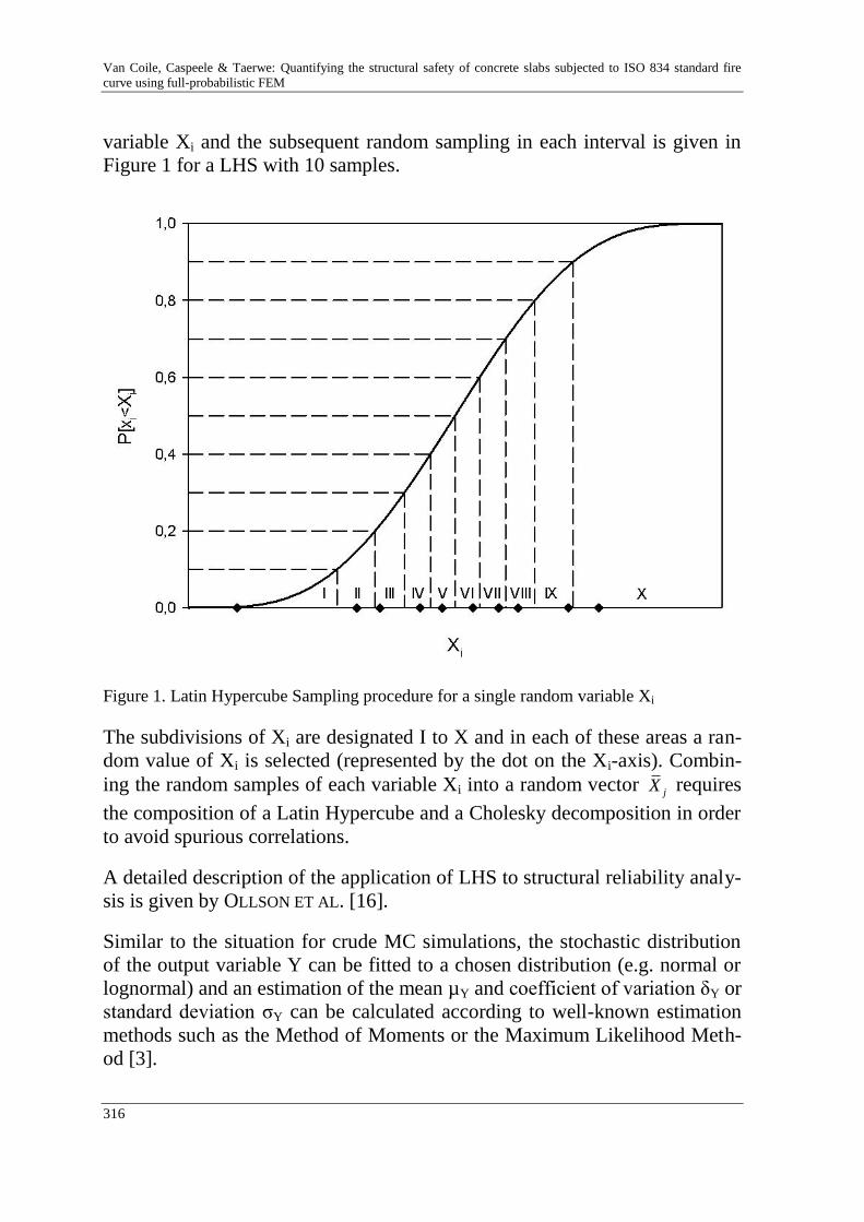
Van Coile, Caspeele & Taerwe: Quantifying the structural safety of concrete slabs subjected to ISO 834 standard fire
curve using full-probabilistic FEM
316
variable Xi and the subsequent random sampling in each interval is given in
Figure 1 for a LHS with 10 samples.
Figure 1. Latin Hypercube Sampling procedure for a single random variable Xi
The subdivisions of Xi are designated I to X and in each of these areas a ran-
dom value of Xi is selected (represented by the dot on the Xi-axis). Combin-
ing the random samples of each variable Xi into a random vector jX requires
the composition of a Latin Hypercube and a Cholesky decomposition in order
to avoid spurious correlations.
A detailed description of the application of LHS to structural reliability analy-
sis is given by OLLSON ET AL. [16].
Similar to the situation for crude MC simulations, the stochastic distribution
of the output variable Y can be fitted to a chosen distribution (e.g. normal or
lognormal) and an estimation of the mean µY and coefficient of variation δY or
standard deviation σY can be calculated according to well-known estimation
methods such as the Method of Moments or the Maximum Likelihood Meth-
od [3].
Moormann, Huber & Proske: Proceedings of the 10th International Probabilistic Workshop, Stuttgart 2012
317
For the set of N simulations performed by LHS, the sample moment m of or-
der r can be calculated by (6) [14] and consequently the mean µY and standard
deviation σY can be estimated by (7) and (8) in accordance with the Method of
Moments [3].
1 r
r jj
m YN
(6)
1ˆ
Y jj
µ m YN
(7)
2 2 2 2 2
,2 ,1 2 1
1ˆ ˆ ˆˆ
Y Y Y j Yj
µ m m YN
(8)
In this study the maximum bending moment capacity of a concrete slab ex-
posed to fire is assessed using the Finite Element software package ATENA.
The following procedure is carried out for each of the N LHS simulations:
1. The LHS samples of the stochastic variables are implemented
2. The slab is subjected to its self-weight
3. The slab is exposed to the ISO 834 standard fire curve for t minutes
4. A load-displacement test is simulated while maintaining the tempera-
ture distribution in the slab
5. Steps 1 to 4 are repeated for different fire exposure durations t
By determining the maximum load bearing capacity for different values of t,
the evolution of the bending moment capacity MR,fi,t during fire is determined
for each of the N slabs. The mean and standard deviation of MR,fi,t is assessed
through (7) and (8). In this study a lognormal distribution for the bending
moment capacity is assumed.

Van Coile, Caspeele & Taerwe: Quantifying the structural safety of concrete slabs subjected to ISO 834 standard fire
curve using full-probabilistic FEM
318
3 Methodology for calculating the reliability index and the fire re-
sistance time
3.1 Calculation of the reliability index
For a concrete slab exposed to fire the limit state function for bending can be
expressed by (9), taking into account that the event of a fire does not affect
the applied load on the concrete slab, in accordance with EN 1992-1-2 [5].
, ,R R fi t E EZ K M K M (9)
with MR,fi,t The bending moment capacity during fire.
ME The bending moment induced by the loads
KR The model uncertainty of the resistance effect
KE The model uncertainty of the load effect
A reliability index βslab is calculated from (9) by a FORM analysis. The bend-
ing moment capacity MR,fi,t is approximated by a lognormal distribution with
mean and coefficient of variation determined by the FEM LHS calculations.
For a concrete slab with a uniformly distributed permanent load gk (character-
istic value) and only a single uniformly distributed variable load qk (character-
istic value), the load ratio χ of the variable load to the total load is defined by
(10) and ME equals MQ + MG, which is correct for a statically determined
concrete slab.
Qkk
k k Qk Gk
Mq
q g M M (10)
with MGk Bending moment induced by gk.
MQk Bending moment induced by qk.
Under ambient design conditions (i.e. at 20°C) and assuming MRd = MEd, the
design value of the bending moment capacity can be calculated by (11),
adapted from EN 1990 [4].
0max ;1 1
Rd Gk G Q G QM M (11)
with G Partial factor for the permaenent load.
Moormann, Huber & Proske: Proceedings of the 10th International Probabilistic Workshop, Stuttgart 2012
319
0 Combination factor
Q Partial factor for the variable load
Reduction factor for unfavorable permanent loads
According to GULVANESSSIAN et al. [6], the permanent load’s characteristic
value can in general be assumed equal to its mean value. Thus, MGk is equal
to its mean value µG and for a given slab configuration (11) defines µG as a
function of the load ratio χ.
The standard deviation σG of the bending moment induced by the permanent
load, and the mean value μQ and standard deviation σQ of the bending moment
induced by the variable loads are calculated through equations (12)-(14), as
suggested in the literature study by HOLICKY and SYKORA [9]. For the bend-
ing moment MG induced by the permanent loads a normal distribution is used,
while for the bending moment MQ induced by the variable load a Gumbel dis-
tribution is assumed [9].
0.1G G (12)
0.6Q QkM (13)
0.35Q Q (14)
The model uncertainty KE of the load effect follows a lognormal distribution
with a mean value of 1 and a standard deviation of 0.1 [9].
It is not clear which model uncertainty KR would be appropriate for non-linear
FEM analysis of concrete elements. For a simplified cross-section calculation,
the model uncertainty KR can be approximated by a lognormal distribution
with mean 1.1 and standard deviation 0.1, based on [10]. Further in this paper
a lognormal model uncertainty KR with mean 1.05 and coefficient of variation
0.1 will be proposed for the FEM calculations. This proposed model uncer-
tainty lies within the boundaries for the model uncertainty for FEM as sug-
gested by SCHLUNE ET AL. [17].

Van Coile, Caspeele & Taerwe: Quantifying the structural safety of concrete slabs subjected to ISO 834 standard fire
curve using full-probabilistic FEM
320
3.2 Evaluation of the design format of EN 1992-1-2 and calculation of
the fire resistance time tR
EN 1992-1-2 [5] defines the structural fire resistance time tR by (3). The par-
tial factors for the calculation of MRd,fi,t and MEd,fi are equal to 1 and a combi-
nation factor fi is prescribed for the variable load.
It is unclear which safety level corresponds with this design format of EN
1992-1-2. However, for a given slab configuration one can calculate a limit
value for the reliability index which is implicitly determined by (3). If the re-
liability index βslab drops below this implicit limit value, the fire resistance
time is reached. The implicit limit value is a function of the time t of fire ex-
posure and will be designated βlimit,EC,t=tR.
Similar to equation (11), the mean bending moment µG* can be calculated for
a given slab configuration and load ratio χ under the assumption MRd,fi,t =
MEd,fi,t and considering the load combination Gk fi QkM M :
*
, , 11
Rd fi t G fiM (15)
with fi Combination factor in case of fire defined by EN 1992-1-2 [5].
The distributions of *
QM and *
GM can similarly be calculated as in equations
(12)-(14). Implementing these distributions in the limit state function (9) for
the time t results in:
* * *
, ,R R fi t E Q GZ K M K M M (16)
Consequently, the limit value βlimit,EC,t=tR for the reliability index is determined
by a FORM calculation.
This methodology allows for an objective evaluation of the design format of
EN 1992-1-2. The following procedure is used for a given slab configuration:
1. For a given time t the design value of the bending moment capacity
during fire MRd,fi,t is calculated.
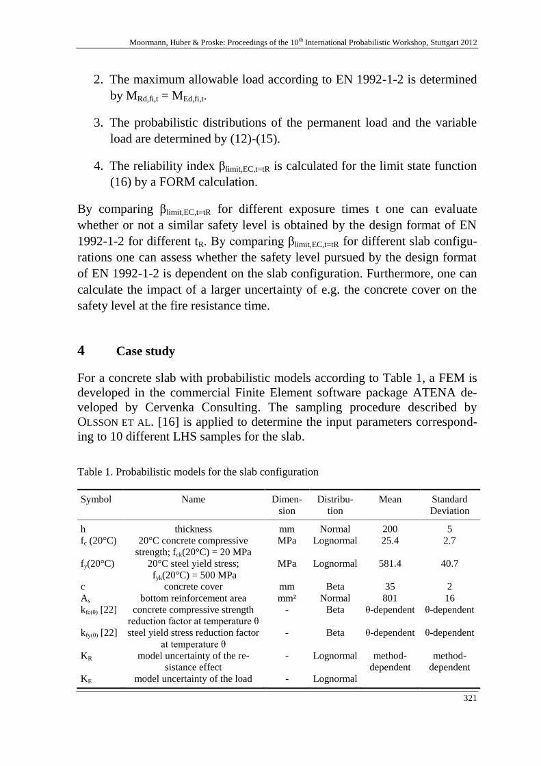
Moormann, Huber & Proske: Proceedings of the 10th International Probabilistic Workshop, Stuttgart 2012
321
2. The maximum allowable load according to EN 1992-1-2 is determined
by MRd,fi,t = MEd,fi,t.
3. The probabilistic distributions of the permanent load and the variable
load are determined by (12)-(15).
4. The reliability index βlimit,EC,t=tR is calculated for the limit state function
(16) by a FORM calculation.
By comparing βlimit,EC,t=tR for different exposure times t one can evaluate
whether or not a similar safety level is obtained by the design format of EN
1992-1-2 for different tR. By comparing βlimit,EC,t=tR for different slab configu-
rations one can assess whether the safety level pursued by the design format
of EN 1992-1-2 is dependent on the slab configuration. Furthermore, one can
calculate the impact of a larger uncertainty of e.g. the concrete cover on the
safety level at the fire resistance time.
4 Case study
For a concrete slab with probabilistic models according to Table 1, a FEM is
developed in the commercial Finite Element software package ATENA de-
veloped by Cervenka Consulting. The sampling procedure described by
OLSSON ET AL. [16] is applied to determine the input parameters correspond-
ing to 10 different LHS samples for the slab.
Table 1. Probabilistic models for the slab configuration
Symbol Name Dimen-
sion
Distribu-
tion
Mean Standard
Deviation
h
fc (20°C)
fy(20°C)
c
As
kfc(θ) [22]
kfy(θ) [22]
KR
KE
thickness
20°C concrete compressive
strength; fck(20°C) = 20 MPa
20°C steel yield stress;
fyk(20°C) = 500 MPa
concrete cover
bottom reinforcement area
concrete compressive strength
reduction factor at temperature θ
steel yield stress reduction factor
at temperature θ
model uncertainty of the re-
sistance effect
model uncertainty of the load
mm
MPa
MPa
mm
mm²
-
-
-
-
Normal
Lognormal
Lognormal
Beta
Normal
Beta
Beta
Lognormal
Lognormal
200
25.4
581.4
35
801
θ-dependent
θ-dependent
method-
dependent
5
2.7
40.7
2
16
θ-dependent
θ-dependent
method-
dependent
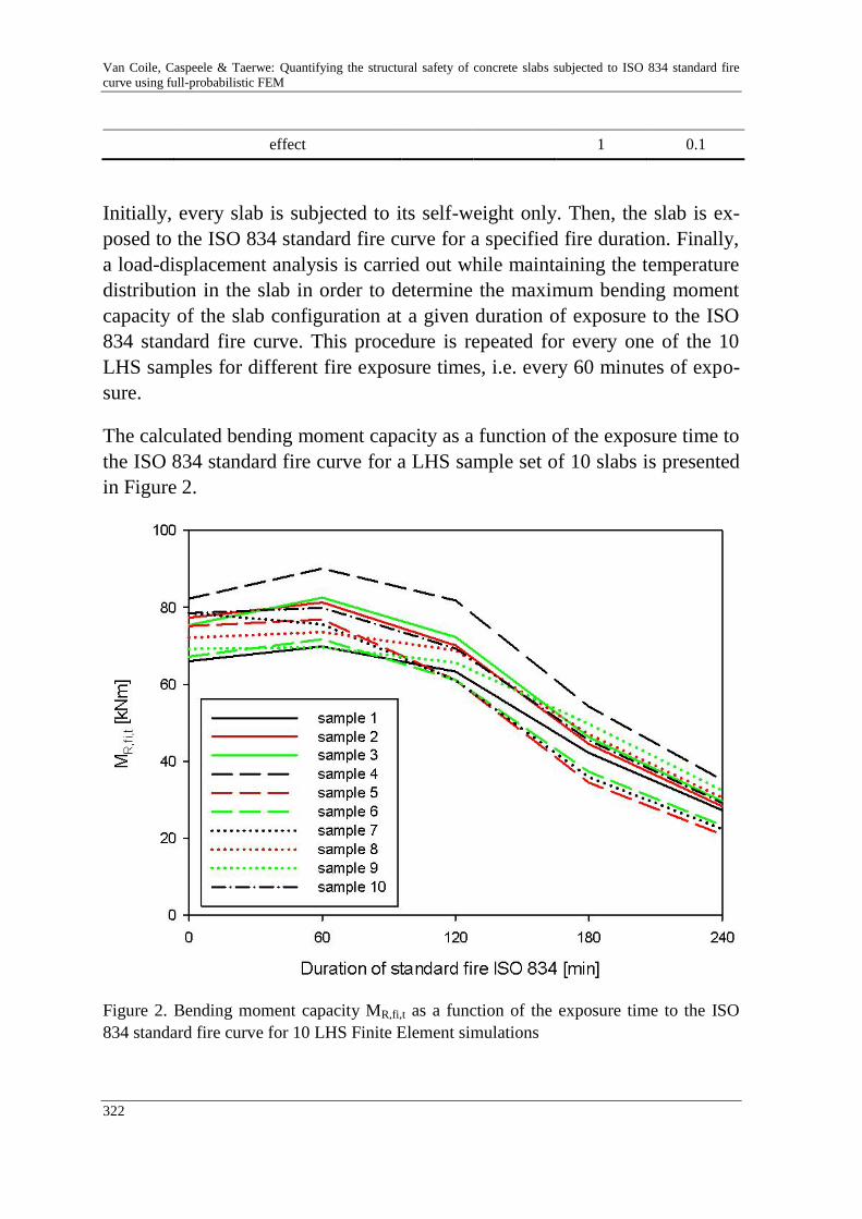
Van Coile, Caspeele & Taerwe: Quantifying the structural safety of concrete slabs subjected to ISO 834 standard fire
curve using full-probabilistic FEM
322
effect 1 0.1
Initially, every slab is subjected to its self-weight only. Then, the slab is ex-
posed to the ISO 834 standard fire curve for a specified fire duration. Finally,
a load-displacement analysis is carried out while maintaining the temperature
distribution in the slab in order to determine the maximum bending moment
capacity of the slab configuration at a given duration of exposure to the ISO
834 standard fire curve. This procedure is repeated for every one of the 10
LHS samples for different fire exposure times, i.e. every 60 minutes of expo-
sure.
The calculated bending moment capacity as a function of the exposure time to
the ISO 834 standard fire curve for a LHS sample set of 10 slabs is presented
in Figure 2.
Figure 2. Bending moment capacity MR,fi,t as a function of the exposure time to the ISO
834 standard fire curve for 10 LHS Finite Element simulations
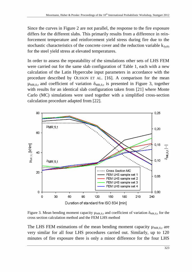
Moormann, Huber & Proske: Proceedings of the 10th International Probabilistic Workshop, Stuttgart 2012
323
Since the curves in Figure 2 are not parallel, the response to the fire exposure
differs for the different slabs. This primarily results from a difference in rein-
forcement temperature and reinforcement yield stress during fire due to the
stochastic characteristics of the concrete cover and the reduction variable kfy(θ)
for the steel yield stress at elevated temperatures.
In order to assess the repeatability of the simulations other sets of LHS FEM
were carried out for the same slab configuration of Table 1, each with a new
calculation of the Latin Hypercube input parameters in accordance with the
procedure described by OLSSON ET AL. [16]. A comparison for the mean
µMR,fi,t and coefficient of variation δMR,fi,t is presented in Figure 3, together
with results for an identical slab configuration taken from [21] where Monte
Carlo (MC) simulations were used together with a simplified cross-section
calculation procedure adapted from [22].
Figure 3. Mean bending moment capacity µMR,fi,t and coefficient of variation δMR,fi,t for the
cross section calculation method and the FEM LHS method
The LHS FEM estimations of the mean bending moment capacity µMR,fi,t are
very similar for all four LHS procedures carried out. Similarly, up to 120
minutes of fire exposure there is only a minor difference for the four LHS
Van Coile, Caspeele & Taerwe: Quantifying the structural safety of concrete slabs subjected to ISO 834 standard fire
curve using full-probabilistic FEM
324
procedures with respect to the coefficient of variation δMR,fi,t. There is howev-
er a larger scatter with respect to δMR,fi,t for fire exposure times exceeding 120
minutes. It is suggested that a small number of samples for the LHS procedure
is sufficient for calculations at lower temperatures, but a larger number of
samples may be required to have a more accurate estimation of the coefficient
of variation during fire.
As can be expected the non-linear FEM calculations indicate a higher average
bending moment capacity than calculated by the simplified cross-section cal-
culations. Furthermore, the strength reserve found by the FEM calculations as
compared to the simplified calculation increases from 5% at 0 minutes of ex-
posure to approximately 35% at 240 minutes of exposure. It is concluded that
the use of a FEM can have significant advantages for the calculation of con-
crete elements exposed to fire.
There is no clear difference in coefficient of variation δMR,fi,t for the cross sec-
tion MC simulations and the LHS FEM. However, a larger number of sam-
ples may be required to have a better estimation of the coefficient of variation
for the LHS FEM procedure.
Assuming a lognormal distribution for the bending moment capacity, equa-
tions (9) and (16) can be evaluated. It is however unclear which model uncer-
tainty KR is appropriate for non-linear FEM analysis [20]. If one calibrates KR
for the specific slab configuration investigated in this paper so that the relia-
bility index βslab for the LHS FEM procedure is approximately equal to βslab
for the simplified MC procedure at 20°C (i.e. at 0 min of exposure to the ISO
834 standard fire curve), a lognormal distribution with mean 1.05 and stand-
ard deviation 0.1 can be proposed, which lies within the boundaries for the
model uncertainty for FEM as suggested by [17]. In Figure 4 the reliability
index at 0 minutes of exposure (i.e. at 20°C) for the four LHS of 10 samples
each and the simplified MC calculation (1000 samples) are presented.
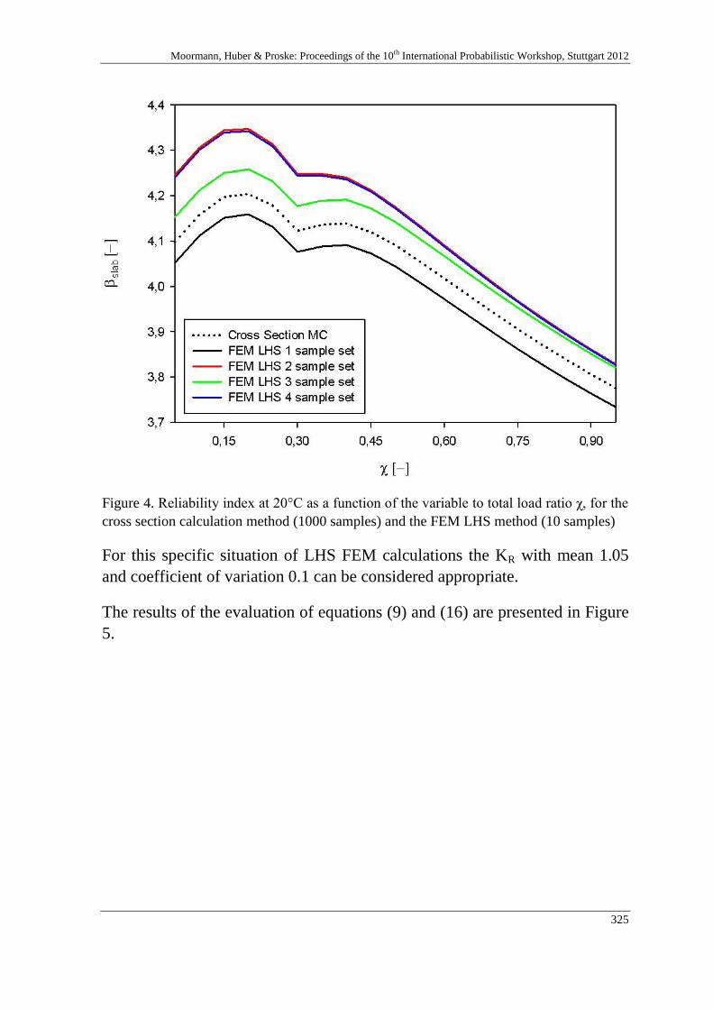
Moormann, Huber & Proske: Proceedings of the 10th International Probabilistic Workshop, Stuttgart 2012
325
Figure 4. Reliability index at 20°C as a function of the variable to total load ratio χ, for the
cross section calculation method (1000 samples) and the FEM LHS method (10 samples)
For this specific situation of LHS FEM calculations the KR with mean 1.05
and coefficient of variation 0.1 can be considered appropriate.
The results of the evaluation of equations (9) and (16) are presented in Figure
5.
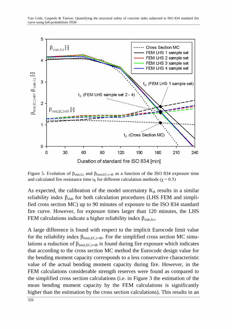
Van Coile, Caspeele & Taerwe: Quantifying the structural safety of concrete slabs subjected to ISO 834 standard fire
curve using full-probabilistic FEM
326
Figure 5. Evolution of βslab,fi,t and βlimit,EC,t=tR as a function of the ISO 834 exposure time
and calculated fire resistance time tR for different calculation methods (χ = 0.5)
As expected, the calibration of the model uncertainty KR results in a similar
reliability index βslab for both calculation procedures (LHS FEM and simpli-
fied cross section MC) up to 90 minutes of exposure to the ISO 834 standard
fire curve. However, for exposure times larger than 120 minutes, the LHS
FEM calculations indicate a higher reliability index βslab,fi,t.
A large difference is found with respect to the implicit Eurocode limit value
for the reliability index βlimit,EC,t=tR. For the simplified cross section MC simu-
lations a reduction of βlimit,EC,t=tR is found during fire exposure which indicates
that according to the cross section MC method the Eurocode design value for
the bending moment capacity corresponds to a less conservative characteristic
value of the actual bending moment capacity during fire. However, in the
FEM calculations considerable strength reserves were found as compared to
the simplified cross section calculations (i.e. in Figure 3 the estimation of the
mean bending moment capacity by the FEM calculations is significantly
higher than the estimation by the cross section calculations). This results in an
Moormann, Huber & Proske: Proceedings of the 10th International Probabilistic Workshop, Stuttgart 2012
327
increase of βlimit,EC,t=tR during fire, which indicates that according to the FEM
calculations, the Eurocode design value during fire corresponds with a more
conservative characteristic of the distribution of the bending moment capaci-
ty.
It should be noted that using the model uncertainty KR for FEM calculations
proposed by JCSS [12], i.e. a lognormal distribution with mean 1.2 and coef-
ficient of variation 0.15 (standard deviation 0.18) results in a significantly
higher estimation of the reliability index at exposure times larger than 120
minutes. Therefore, the model uncertainty proposed by JCSS is found to be
unsafe for these specific calculations. A literature study on model uncertain-
ties by SYKORA ET AL. [20] illustrates that there is currently no consensus on
the model uncertainty to be used for FEM calculations.
The structural fire resistance time tR is determined by the intersection of
βslab,fi,t and βlimit,EC,t=tR. In Figure 5 βslab,fi,t is defined by the assumption that MRd
= MEd at ambient conditions (i.e. at 20°C). Both calculation methods and all
LHS FEM calculations result in approximately the same fire resistance time
tR, but a difference is found for the reliability index at the fire resistance time.
It is concluded that the proposed methodology allows for an objective com-
parison of different design alternatives with respect to the fire resistance time
tR, irrespective of the calculation procedure used. This property can be of in-
terest for structural fire safety engineering when using FEM to design equiva-
lent solutions to prescriptive codes based on simple cross section calculations.
The FEM calculations indicate a higher reliability index β at the fire re-
sistance time as compared to simplified cross section calculations. Therefore
FEM calculations of concrete elements exposed to fire can constitute consid-
erable advantages when performing a reliability optimization.
5 Conclusions
The combination of Latin Hypercube Sampling and non-linear Finite
Element Models is found to be an efficient calculation procedure for
the analysis of concrete elements exposed to fire.
At 20°C the mean bending moment capacity calculated by the FEM
procedure is only slightly higher than the one determined by a simpli-
fied cross-section calculation. However, during fire the FEM calcula-
Van Coile, Caspeele & Taerwe: Quantifying the structural safety of concrete slabs subjected to ISO 834 standard fire
curve using full-probabilistic FEM
328
tions result in a significantly higher bending moment capacity, indicat-
ing that FEM calculations for concrete elements exposed to fire can
have considerable advantages for design.
There is currently no consensus on the model uncertainty KR for the re-
sistance effect to be used for non-linear FEM calculations at 20°C. A
lognormal distribution with mean 1.05 and coefficient of variation 0.1
is proposed for the specific situation investigated, chosen according to
the suggestions found in literature. However it is questionable whether
the same model uncertainty is appropriate at elevated temperatures.
A probabilistic procedure for the calculation of the structural fire re-
sistance time tR is proposed which allows for an objective comparison
of different design alternatives. With respect to tR, the proposed meth-
odology is found to be independent of the calculation method used (Fi-
nite Element Model or simplified cross section calculation method).
However, the FEM calculations indicate a higher reliability index β at
the fire resistance time as compared to simplified cross section calcula-
tions. Therefore FEM calculations of concrete elements exposed to fire
can constitute considerable advantages when performing a reliability
optimization.
6 Acknowledgements
RUBEN VAN COILE is a Research Assistant of the FWO Research Foundation
Flanders. The authors wish to thank the FWO for the financial support on the
research project “Probabilistic Formulation of the structural reliability of con-
crete structures subjected to fire in relation to risk-based decision making and
risk-transfer mechanisms”.
7 References
[1] Ang, A.H.-S.; Tang, W.H., Probability concepts in engineering (2nd
edition). John
Wiley & Sons, 2007
[2] Au, S.K.; Wang, Z.-H.; Lo, S.-M.: Compartment fire risk analysis by advanced Mon-
te Carlo simulation. Engineering Structures, 29 (2007), p. 2381-2390
Moormann, Huber & Proske: Proceedings of the 10th International Probabilistic Workshop, Stuttgart 2012
329
[3] Benjamin, J.R.; Cornell, C.A.: Probability, Statistics and Decision for Civil Engi-
neers. McGraw-Hill, 1970
[4] CEN.: European Standard EN 1990: Eurocode 0: Basis of structural design. Brus-
sels, 2002
[5] CEN.: European Standard EN 1992-1-2: Eurocode 2: Design of concrete structures:
Part 1-2: Structural fire design. Brussels, 2004.
[6] Gulvanessian, H.; Calgaro, J.-A.; Holický, M.: Designer’s guide to EN 1990: Eur-
code 0: Basis for structural design. Thomas Telford, 2002
[7] Guo, Q.; Jeffers, A.E.: Finite Element Reliability Analysis for Structural Safety
Evaluation in Fire. In: Fontana, M.; Frangi, A.; Knobloch, M. (eds): Proceedings of
the 7th
International Conference on Structures in Fire. Zürich, 2012, p. 469-478
[8] Hasofer, A.M.; Qu, J.: Response surface modelling of monte carlo fire data. Fire
Safety Journal 37 (2002), p. 772-784
[9] Holický, M.; Sýkora, M.: Stochastic models in analysis of structural reliability. Pro-
ceedings of the International Symposium on Stochastic Models in Reliability Engi-
neering, Life Sciences and Operation Management. Beer Sheva, 2010
[10] Holický, M.; Retief, J.V.; Dunaiski, P.E.: The reliability basis of design for structural
resistance. Proceedings of the Third International Conference on Structural Engi-
neering, Mechanics and Computation (SEMC). Cape Town, 2007
[11] ISO 834, Fire Resistance Tests – Elements of Buildings Construction – Part I - Gen-
eral Requirement, 1999
[12] Joint Committee on Structural Safety: JCSS Probabilistic Model Code,
www.jcss.byg.dtu.dk, Zürich, 2006
[13] Kang, S.-C.; Koh, H.-M.; Choo, J.F.: An efficient response surface method using
moving least squares approximation for structural reliability analysis. Probabilistic
Engineering Mechanics, 25 (2010), p. 365-371
[14] Keramat, M.; Kielbasa, R.: Latin Hypercube Sampling Monte Carlo Estimation of
Average Quality Index for Integrated Circuits. Analog Integrated Circuits And Signal
Processing 14 (1997), p. 131-142
[15] Novák, D.; Vorechovský, M.; Lehký, D.; Rusina, R.; Pukl, R.; Cervenka, V.: Sto-
chastic nonlinear fracture mechanics finite element analysis of concrete structures.
Proceedings of the 9th
International Conference on Structural Safety and Reliability
(ICOSSAR). Rome, 2005, p. 781-788
Van Coile, Caspeele & Taerwe: Quantifying the structural safety of concrete slabs subjected to ISO 834 standard fire
curve using full-probabilistic FEM
330
[16] Olsson, A.; Sandberg, G.; Dahlblom, O.: On Latin Hypercube Sampling for Structur-
al Reliability Analysis. Structural Safety 25 (2003), p. 47-68
[17] Schlune, H.; Plos, M.; Gylltoft, K.: Safety formats for nonlinear analysis tested on
concrete beams subjected to shear forces and bending moments. Engineering Struc-
tures, 33 (2011), p. 2350-2356
[18] Shi, K.; Guo, Q.; Jeffers, A.E.: Stochastic analysis of structures in fire by Monte Car-
lo simulation. In: Wald, F; Horová, K.; Jirku, J. (eds.): Proceedings of the Applica-
tion of Structural Fire Engineering Conference (ASFE). Prague, 2011, p. 355-360
[19] Sidibé, K., Duprat, F., Pinglot, M. and Bourret, B., Fire Safety of Reinforced Con-
crete Columns, ACI Structural Journal, 97 (2000), p. 642-647
[20] Sýkora, M.; Cervenka, V.; Holický, M.: Assessment of model uncertainties in the
analysis of reinforced concrete structures. In: Naprstek, J.; Fischer, C. (eds): Pro-
ceedings of the 18th
International Conference on Engineering Mechanics. Svratka,
2012
[21] Van Coile, R.; Caspeele, R.; Taerwe, L.: Global Resistance Factor for Concrete Slabs
exposed to Fire, In: Fontana, M.; Frangi, A.; Knobloch, M. (eds): Proceedings of the
7th
International Conference on Structures in Fire. Zürich, 2012, p. 775-784
[22] Van Coile, R.; Annerel, E.; Caspeele, R.; Taerwe, L.: Assessment of the safety level
of concrete slabs during fire. Fire Safety Science – Proceedings of the 10th
Interna-
tional Symposium. Maryland, 2011, 1115-1124
[23] Van Coile, R.; Caspeele, R.; Annerel, E.; Taerwe, L.: Assessment of the reduction of
the safety level of concrete slabs during fire. In: Gucma, L.; Van Gelder, P.; Proske,
D. (eds.): Proceedings of the 8th
International Probabilistic Workshop. Szczecin,
2010, p. 61-72

Moormann, Huber & Proske: Proceedings of the 10th International Probabilistic Workshop, Stuttgart 2012
331
Reliability of a crankshaft by using Markov
chain model with a probabilistic approach.
Nik Abdullah Nik Mohamed, Salvinder Singh Karam Singh
Faculty of Engineering and Built Environment, Department of Mechanical
Engineering, Universiti Kebangsaan Malaysia, Malaysia.
Mohd Salmi Md Noorani
Faculty of Science and Technology, Universiti Kebangsaan Malaysia,
Malaysia.
Abstract: This paper describes the probabilistic method of using Markov chain model to
determine the reliability of the crankshaft based on the Weibull distribution. The
crankshafts are constantly subjected to cyclic loading which will tend to display the effects
of fatigue which is stochastic in nature. The bending stresses are due to self-weight of the
piston, connecting rod and other components or misalignment of the piston and torsion
stress. Therefore, the fatigue failures generally are of the rotating bending type and
torsional based on the nature of its working condition. The Markov chain model was
constructed and the probability method was selected to represent the bending and torsion
loads acting on the crankshaft for a range of operating hours. The criteria for probability
loading for bending would be higher compared to torsion because the initial loading for the
crankshaft is bending due to its working condition. Based from the Markov chain model,
the shape and scale parameter was calculated and was used to determine the Weibull
probability density function, cumulative distribution function, hazard rate and hazard rate-
reliability. It was observed from the characteristic of the Weibull shape parameter that the
failure due to bending-torsion was an increasing failure rate (IFR) with the mean load to
failure (MLTF) 3.4 MPa. This can be seen from the behaviour of the crack that shows it
propagates from the fillet region towards the oil seal at a 45 degree angle.
1 Introduction
In this paper, the concept of probabilistic approach will be introduced by
using the Markov chain model in determining the failure of a crankshaft based
on bending and torsional loading. The aim of this paper was to develop the
reliability and statistical analysis on the crankshaft by using the Markov chain
model based on the applied loads. The development of the probabilistic
approach by using this model provides an alternative method in determining
Nik Abdullah, Salvinder & Salmi : Reliability of a crankshaft by using Markov chain model with a
probabilistic approach.
332
the failure of the crankshaft, whereby this model looks at a sequence of
events, and analyzes the tendency of one event to be followed by another.
From the developed Markov chain model, a new sequence of random but
related events, which will look similar to the original event, was generated.
The model developed was useful in analyzing dependent random events - that
is, events whose likelihood depends on what happened last over a transition
time.
Bending and torsion are main types of loading that will occur on the
crankshaft. The failures acting on the crankshaft are generally of the torsional
and rotating bending based on the nature of its working condition. The
operating condition of the crankshaft is that it will rotate at 720 degree for a
complete 4-stroke cycle which consist of the intake, combustion, power and
exhaust stoke. During the combustion and power cycle the pressure acting on
the piston head will be the highest where the compressed air–fuel mixture will
be ignited, usually by a spark plug, which in return will be ignited due to the
heat generated from the air-fuel mixture during the compression stroke. This
resulting massive pressure from the combustion of the compressed fuel-air
mixture forces the piston back down toward bottom dead centre based on
operating procedure of the crankshaft.
Salvatore et al. [12] mentioned that the reliability of the crankshaft is the
construction of the model that can be represented by the time to failure of the
crankshaft based on the distribution of load. From the reliability point of
view, it is possible that the crankshaft has influence on other sub-components
of the vehicle such as the connecting rod and the engine block. This can be
used in characterising the reliability dynamics of the crankshaft.
Hyun Jung et al. [5] mentioned that the crankshaft is the core element of the
engine of a vehicle, that transforms the translation motion generated by com-
bustion to rotational motion. Therefore the failure of crankshaft can cause
serious damage to the engine even though the crankshaft must be designed to
last a lifetime of an engine. Hyun Jung et al. [5] also did mention that practi-
cal case and investigation revealed that bending stress is much serve than tor-
sion. The fillet region is the highest point of stress on the crankshaft due to
loads from bending and torsion simultaneously. The failure due to cracks at
the fillet region starts from the fillet region and will propagate along the jour-
nal to the oilseal due to irregularities during the manufacturing process.
Asi [10] mentioned that the main reason of failure in a crankshaft is due to the
cyclic loading during rotation on its axis. The crankshaft is normally
subjected to bending stresses due to self-weight of the piston, connecting rod
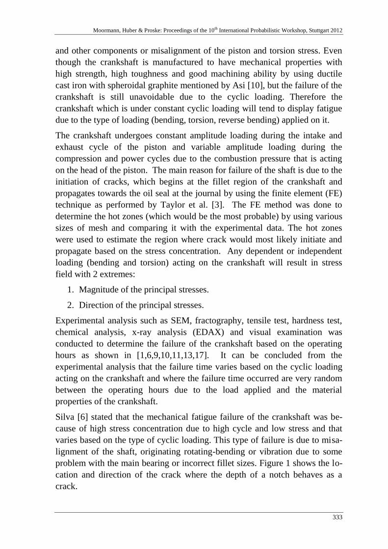
Moormann, Huber & Proske: Proceedings of the 10th International Probabilistic Workshop, Stuttgart 2012
333
and other components or misalignment of the piston and torsion stress. Even
though the crankshaft is manufactured to have mechanical properties with
high strength, high toughness and good machining ability by using ductile
cast iron with spheroidal graphite mentioned by Asi [10], but the failure of the
crankshaft is still unavoidable due to the cyclic loading. Therefore the
crankshaft which is under constant cyclic loading will tend to display fatigue
due to the type of loading (bending, torsion, reverse bending) applied on it.
The crankshaft undergoes constant amplitude loading during the intake and
exhaust cycle of the piston and variable amplitude loading during the
compression and power cycles due to the combustion pressure that is acting
on the head of the piston. The main reason for failure of the shaft is due to the
initiation of cracks, which begins at the fillet region of the crankshaft and
propagates towards the oil seal at the journal by using the finite element (FE)
technique as performed by Taylor et al. [3]. The FE method was done to
determine the hot zones (which would be the most probable) by using various
sizes of mesh and comparing it with the experimental data. The hot zones
were used to estimate the region where crack would most likely initiate and
propagate based on the stress concentration. Any dependent or independent
loading (bending and torsion) acting on the crankshaft will result in stress
field with 2 extremes:
1. Magnitude of the principal stresses.
2. Direction of the principal stresses.
Experimental analysis such as SEM, fractography, tensile test, hardness test,
chemical analysis, x-ray analysis (EDAX) and visual examination was
conducted to determine the failure of the crankshaft based on the operating
hours as shown in [1,6,9,10,11,13,17]. It can be concluded from the
experimental analysis that the failure time varies based on the cyclic loading
acting on the crankshaft and where the failure time occurred are very random
between the operating hours due to the load applied and the material
properties of the crankshaft.
Silva [6] stated that the mechanical fatigue failure of the crankshaft was be-
cause of high stress concentration due to high cycle and low stress and that
varies based on the type of cyclic loading. This type of failure is due to misa-
lignment of the shaft, originating rotating-bending or vibration due to some
problem with the main bearing or incorrect fillet sizes. Figure 1 shows the lo-
cation and direction of the crack where the depth of a notch behaves as a
crack.
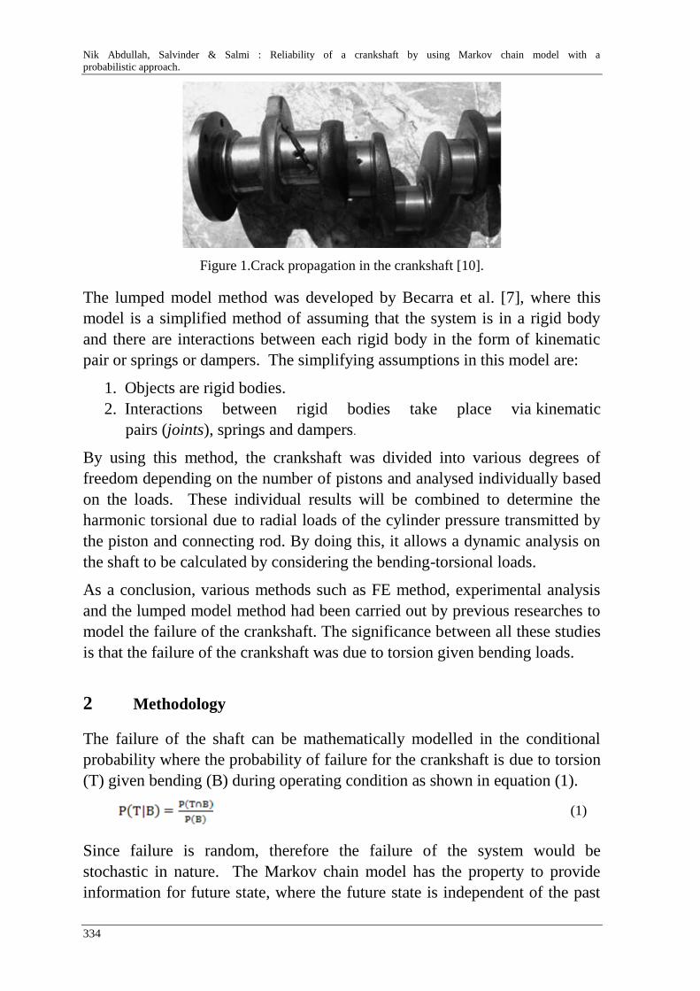
Nik Abdullah, Salvinder & Salmi : Reliability of a crankshaft by using Markov chain model with a
probabilistic approach.
334
Figure 1.Crack propagation in the crankshaft [10].
The lumped model method was developed by Becarra et al. [7], where this
model is a simplified method of assuming that the system is in a rigid body
and there are interactions between each rigid body in the form of kinematic
pair or springs or dampers. The simplifying assumptions in this model are:
1. Objects are rigid bodies.
2. Interactions between rigid bodies take place via kinematic
pairs (joints), springs and dampers.
By using this method, the crankshaft was divided into various degrees of
freedom depending on the number of pistons and analysed individually based
on the loads. These individual results will be combined to determine the
harmonic torsional due to radial loads of the cylinder pressure transmitted by
the piston and connecting rod. By doing this, it allows a dynamic analysis on
the shaft to be calculated by considering the bending-torsional loads.
As a conclusion, various methods such as FE method, experimental analysis
and the lumped model method had been carried out by previous researches to
model the failure of the crankshaft. The significance between all these studies
is that the failure of the crankshaft was due to torsion given bending loads.
2 Methodology
The failure of the shaft can be mathematically modelled in the conditional
probability where the probability of failure for the crankshaft is due to torsion
(T) given bending (B) during operating condition as shown in equation (1).
(1)
Since failure is random, therefore the failure of the system would be
stochastic in nature. The Markov chain model has the property to provide
information for future state, where the future state is independent of the past

Moormann, Huber & Proske: Proceedings of the 10th International Probabilistic Workshop, Stuttgart 2012
335
state given that we know the present state, which has the similar properties of
the crankshaft under operating condition.
The Markov chain model for loading on the crankshaft system was set in two
states, i.e. bending and torsion as shown in Figure 2. This model is in the
recurrent state whereby the loading of bending and torsion will be repeating
over time.
Figure 2. Markov chain state diagram of the crankshaft
The probabilistic equation of the Markov chain from Figure 2 can be
modelled as a memoryless condition based on equation (2), where it describes
the probability (Pr) of going from the bending state to the torsion state and
vice versa was based only on the given present state regardless of its past
condition.
(2)
Each probability matrices of bending (PB) and torsion, (PT) is set to be
independent of each other where each of the probability of failure due to
bending and torsion is a compliment of each other. In other words, for each
PT, it will contain the remaining PB and vice-versa for PT, as shown in
equation (3).
(3)
The torsion loading would only start to take effect when the crankshaft is in
the operating condition, due to rotation on its axis. Hence, the probability
matrix for the crankshaft (P) based on the operating hours (n) can be
illustrated in equation (4).
(4)
The Chapman-Kolmogorov method as shown in equation (5) was derived to
observe the changes that would over the loading states as time increases
whereby the outcome of each transition time is independent on its initial
condition. This was done to observe was there any steady state condition for
the probability matrix provided.
Probability of torsion
Probability of bending
B T
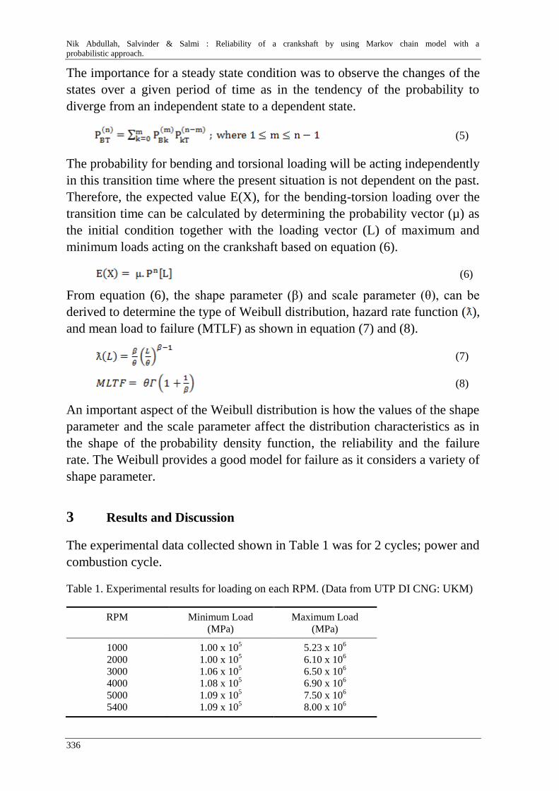
Nik Abdullah, Salvinder & Salmi : Reliability of a crankshaft by using Markov chain model with a
probabilistic approach.
336
The importance for a steady state condition was to observe the changes of the
states over a given period of time as in the tendency of the probability to
diverge from an independent state to a dependent state.
(5)
The probability for bending and torsional loading will be acting independently
in this transition time where the present situation is not dependent on the past.
Therefore, the expected value E(X), for the bending-torsion loading over the
transition time can be calculated by determining the probability vector (µ) as
the initial condition together with the loading vector (L) of maximum and
minimum loads acting on the crankshaft based on equation (6).
(6)
From equation (6), the shape parameter (β) and scale parameter (θ), can be
derived to determine the type of Weibull distribution, hazard rate function ( ),
and mean load to failure (MTLF) as shown in equation (7) and (8).
(7)
(8)
An important aspect of the Weibull distribution is how the values of the shape
parameter and the scale parameter affect the distribution characteristics as in
the shape of the probability density function, the reliability and the failure
rate. The Weibull provides a good model for failure as it considers a variety of
shape parameter.
3 Results and Discussion
The experimental data collected shown in Table 1 was for 2 cycles; power and
combustion cycle.
Table 1. Experimental results for loading on each RPM. (Data from UTP DI CNG: UKM)
RPM Minimum Load
(MPa)
Maximum Load
(MPa)
1000
2000
3000
4000
5000
5400
1.00 x 10⁵
1.00 x 10⁵
1.06 x 10⁵
1.08 x 10⁵
1.09 x 10⁵
1.09 x 10⁵
5.23 x 10⁶
6.10 x 10⁶
6.50 x 10⁶
6.90 x 10⁶
7.50 x 10⁶
8.00 x 10⁶
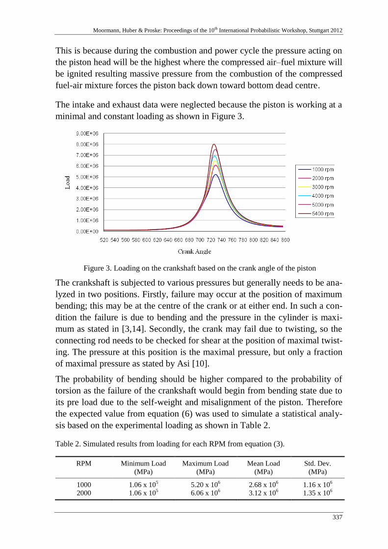
Moormann, Huber & Proske: Proceedings of the 10th International Probabilistic Workshop, Stuttgart 2012
337
This is because during the combustion and power cycle the pressure acting on
the piston head will be the highest where the compressed air–fuel mixture will
be ignited resulting massive pressure from the combustion of the compressed
fuel-air mixture forces the piston back down toward bottom dead centre.
The intake and exhaust data were neglected because the piston is working at a
minimal and constant loading as shown in Figure 3.
Figure 3. Loading on the crankshaft based on the crank angle of the piston
The crankshaft is subjected to various pressures but generally needs to be ana-
lyzed in two positions. Firstly, failure may occur at the position of maximum
bending; this may be at the centre of the crank or at either end. In such a con-
dition the failure is due to bending and the pressure in the cylinder is maxi-
mum as stated in [3,14]. Secondly, the crank may fail due to twisting, so the
connecting rod needs to be checked for shear at the position of maximal twist-
ing. The pressure at this position is the maximal pressure, but only a fraction
of maximal pressure as stated by Asi [10].
The probability of bending should be higher compared to the probability of
torsion as the failure of the crankshaft would begin from bending state due to
its pre load due to the self-weight and misalignment of the piston. Therefore
the expected value from equation (6) was used to simulate a statistical analy-
sis based on the experimental loading as shown in Table 2.
Table 2. Simulated results from loading for each RPM from equation (3).
RPM Minimum Load
(MPa)
Maximum Load
(MPa)
Mean Load
(MPa)
Std. Dev.
(MPa)
1000
2000
1.06 x 10⁵
1.06 x 10⁵
5.20 x 10⁶
6.06 x 10⁶
2.68 x 10⁶
3.12 x 10⁶
1.16 x 10⁶
1.35 x 10⁶
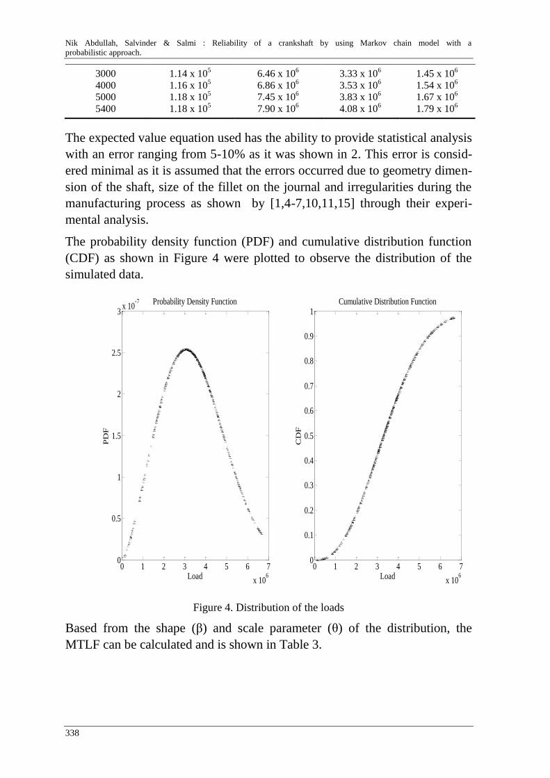
Nik Abdullah, Salvinder & Salmi : Reliability of a crankshaft by using Markov chain model with a
probabilistic approach.
338
3000
4000
5000
5400
1.14 x 10⁵
1.16 x 10⁵
1.18 x 10⁵
1.18 x 10⁵
6.46 x 10⁶
6.86 x 10⁶
7.45 x 10⁶
7.90 x 10⁶
3.33 x 10⁶
3.53 x 10⁶
3.83 x 10⁶
4.08 x 10⁶
1.45 x 10⁶
1.54 x 10⁶
1.67 x 10⁶
1.79 x 10⁶
The expected value equation used has the ability to provide statistical analysis
with an error ranging from 5-10% as it was shown in 2. This error is consid-
ered minimal as it is assumed that the errors occurred due to geometry dimen-
sion of the shaft, size of the fillet on the journal and irregularities during the
manufacturing process as shown by [1,4-7,10,11,15] through their experi-
mental analysis.
The probability density function (PDF) and cumulative distribution function
(CDF) as shown in Figure 4 were plotted to observe the distribution of the
simulated data.
0 1 2 3 4 5 6 7
x 106
0
0.5
1
1.5
2
2.5
3x 10
-7
Load
PD
F
Probability Density Function
0 1 2 3 4 5 6 7
x 106
0
0.1
0.2
0.3
0.4
0.5
0.6
0.7
0.8
0.9
1
Load
CD
FCumulative Distribution Function
Figure 4. Distribution of the loads
Based from the shape (β) and scale parameter (θ) of the distribution, the
MTLF can be calculated and is shown in Table 3.
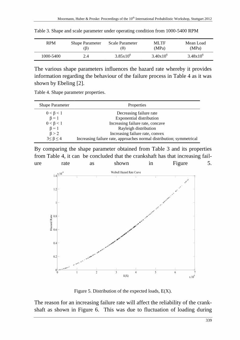
Moormann, Huber & Proske: Proceedings of the 10th International Probabilistic Workshop, Stuttgart 2012
339
Table 3. Shape and scale parameter under operating condition from 1000-5400 RPM
RPM Shape Parameter
(β)
Scale Parameter
(θ)
MLTF
(MPa)
Mean Load
(MPa)
1000-5400 2.4 3.85x10⁶
3.40x10⁶
3.48x10⁶
The various shape parameters influences the hazard rate whereby it provides
information regarding the behaviour of the failure process in Table 4 as it was
shown by Ebeling [2].
Table 4. Shape parameter properties.
Shape Parameter Properties
0 < β < 1
β = 1
0 < β < 1
β = 1
β > 2
3≤ β ≤ 4
Decreasing failure rate
Exponential distribution
Increasing failure rate, concave
Rayleigh distribution
Increasing failure rate, convex
Increasing failure rate, approaches normal distribution; symmetrical
By comparing the shape parameter obtained from Table 3 and its properties
from Table 4, it can be concluded that the crankshaft has that increasing fail-
ure rate as shown in Figure 5.
0 1 2 3 4 5 6 7
x 106
0
0.2
0.4
0.6
0.8
1
1.2
1.4x 10
-6
E(X)
Hazard
Rate
Weibull Hazard Rate Curve
Figure 5. Distribution of the expected loads, E(X).
The reason for an increasing failure rate will affect the reliability of the crank-
shaft as shown in Figure 6. This was due to fluctuation of loading during
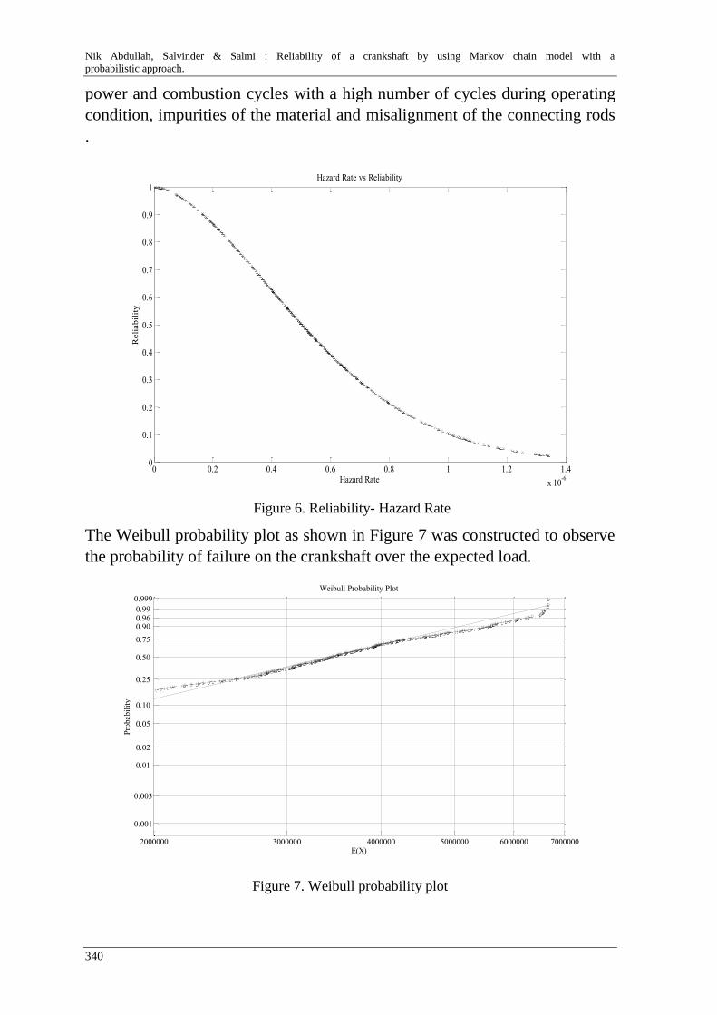
Nik Abdullah, Salvinder & Salmi : Reliability of a crankshaft by using Markov chain model with a
probabilistic approach.
340
power and combustion cycles with a high number of cycles during operating
condition, impurities of the material and misalignment of the connecting rods
.
0 0.2 0.4 0.6 0.8 1 1.2 1.4
x 10-6
0
0.1
0.2
0.3
0.4
0.5
0.6
0.7
0.8
0.9
1
Hazard Rate
Reli
abil
ity
Hazard Rate vs Reliability
Figure 6. Reliability- Hazard Rate
The Weibull probability plot as shown in Figure 7 was constructed to observe
the probability of failure on the crankshaft over the expected load.
2000000 3000000 4000000 5000000 6000000 7000000
0.001
0.003
0.01
0.02
0.05
0.10
0.25
0.50
0.75
0.90 0.96 0.99
0.999
E(X)
Pro
bab
ilit
y
Weibull Probability Plot
Figure 7. Weibull probability plot
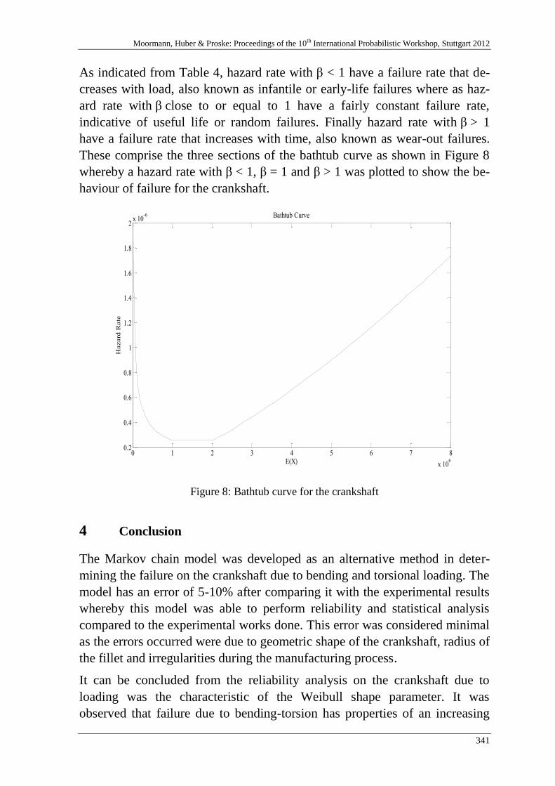
Moormann, Huber & Proske: Proceedings of the 10th International Probabilistic Workshop, Stuttgart 2012
341
As indicated from Table 4, hazard rate with β < 1 have a failure rate that de-
creases with load, also known as infantile or early-life failures where as haz-
ard rate with β close to or equal to 1 have a fairly constant failure rate,
indicative of useful life or random failures. Finally hazard rate with β > 1
have a failure rate that increases with time, also known as wear-out failures.
These comprise the three sections of the bathtub curve as shown in Figure 8
whereby a hazard rate with β < 1, β = 1 and β > 1 was plotted to show the be-
haviour of failure for the crankshaft.
0 1 2 3 4 5 6 7 8
x 106
0.2
0.4
0.6
0.8
1
1.2
1.4
1.6
1.8
2x 10
-6
E(X)
Hazard
Rate
Bathtub Curve
Figure 8: Bathtub curve for the crankshaft
4 Conclusion
The Markov chain model was developed as an alternative method in deter-
mining the failure on the crankshaft due to bending and torsional loading. The
model has an error of 5-10% after comparing it with the experimental results
whereby this model was able to perform reliability and statistical analysis
compared to the experimental works done. This error was considered minimal
as the errors occurred were due to geometric shape of the crankshaft, radius of
the fillet and irregularities during the manufacturing process.
It can be concluded from the reliability analysis on the crankshaft due to
loading was the characteristic of the Weibull shape parameter. It was
observed that failure due to bending-torsion has properties of an increasing
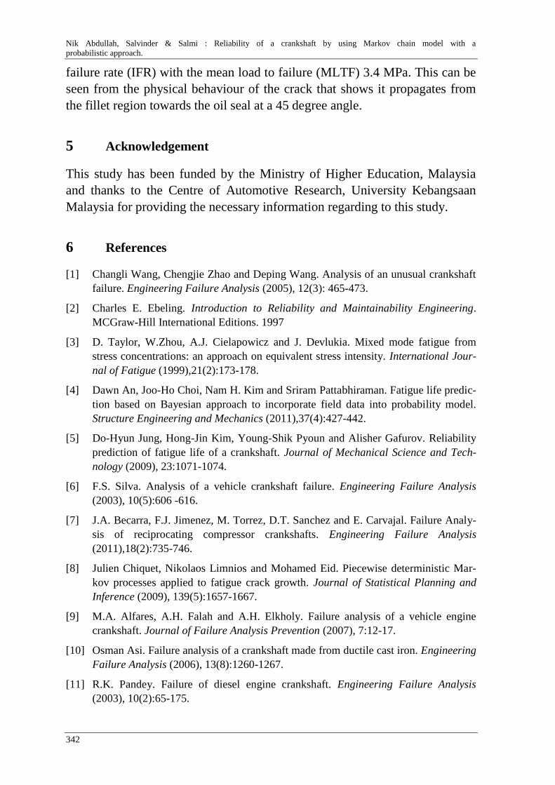
Nik Abdullah, Salvinder & Salmi : Reliability of a crankshaft by using Markov chain model with a
probabilistic approach.
342
failure rate (IFR) with the mean load to failure (MLTF) 3.4 MPa. This can be
seen from the physical behaviour of the crack that shows it propagates from
the fillet region towards the oil seal at a 45 degree angle.
5 Acknowledgement
This study has been funded by the Ministry of Higher Education, Malaysia
and thanks to the Centre of Automotive Research, University Kebangsaan
Malaysia for providing the necessary information regarding to this study.
6 References
[1] Changli Wang, Chengjie Zhao and Deping Wang. Analysis of an unusual crankshaft
failure. Engineering Failure Analysis (2005), 12(3): 465-473.
[2] Charles E. Ebeling. Introduction to Reliability and Maintainability Engineering.
MCGraw-Hill International Editions. 1997
[3] D. Taylor, W.Zhou, A.J. Cielapowicz and J. Devlukia. Mixed mode fatigue from
stress concentrations: an approach on equivalent stress intensity. International Jour-
nal of Fatigue (1999),21(2):173-178.
[4] Dawn An, Joo-Ho Choi, Nam H. Kim and Sriram Pattabhiraman. Fatigue life predic-
tion based on Bayesian approach to incorporate field data into probability model.
Structure Engineering and Mechanics (2011),37(4):427-442.
[5] Do-Hyun Jung, Hong-Jin Kim, Young-Shik Pyoun and Alisher Gafurov. Reliability
prediction of fatigue life of a crankshaft. Journal of Mechanical Science and Tech-
nology (2009), 23:1071-1074.
[6] F.S. Silva. Analysis of a vehicle crankshaft failure. Engineering Failure Analysis
(2003), 10(5):606 -616.
[7] J.A. Becarra, F.J. Jimenez, M. Torrez, D.T. Sanchez and E. Carvajal. Failure Analy-
sis of reciprocating compressor crankshafts. Engineering Failure Analysis
(2011),18(2):735-746.
[8] Julien Chiquet, Nikolaos Limnios and Mohamed Eid. Piecewise deterministic Mar-
kov processes applied to fatigue crack growth. Journal of Statistical Planning and
Inference (2009), 139(5):1657-1667.
[9] M.A. Alfares, A.H. Falah and A.H. Elkholy. Failure analysis of a vehicle engine
crankshaft. Journal of Failure Analysis Prevention (2007), 7:12-17.
[10] Osman Asi. Failure analysis of a crankshaft made from ductile cast iron. Engineering
Failure Analysis (2006), 13(8):1260-1267.
[11] R.K. Pandey. Failure of diesel engine crankshaft. Engineering Failure Analysis
(2003), 10(2):65-175.

Moormann, Huber & Proske: Proceedings of the 10th International Probabilistic Workshop, Stuttgart 2012
343
[12] Salvatore Distefano and Antonio Peliafito. Reliability and avaliability of dependent
dynamic system with DRBD’s. Reliability Engineering and System Safety (2009),
94(9):1381-1393.
[13] S.K. Bahumik, R. Rangaraju, M.A. Venkataswamy, T.A. Baskaran and M.A.
Parameswara. Fatigue fracture of crankshaft of an aircraft engine. Engineering Fail-
ure Analysis (2002), 9:255-263.
[14] W.F. Wu and C.C. Ni. Probabilistic models of fatigue crack propagation and their
experimental verification. Probabilistic Engineering Mechanics (2004), 19(3):247-
257.
[15] W.Y. Chien, J.Pan, D.Close and S.Ho. Fatigue analysis of crankshaft under bending
with consideration of residual stresses. International Journal of Fatigue (2005),
27(1):1-19.
[16] Xuanyang Lei, Guicai ZhPang, Ji Chen, Song Xigeng and Guangming Dong. Simu-
lation on the motion of crankshaft with a slant crack in crankpin. Mechanical Systems
and Signal and Processing (2007), 21:502-513.
[17] Zissimos P. Mourelatos. A crankshaft system model for structural dynamic analysis
of internal combustion engines. Computers and Structures (2001),79:2009-2027.

Nik Abdullah, Salvinder & Salmi : Reliability of a crankshaft by using Markov chain model with a
probabilistic approach.
344

Moormann, Huber & Proske: Proceedings of the 10th International Probabilistic Workshop, Stuttgart 2012
345
Probabilistic assessment of existing structures
Milan Holický, Miroslav Sýkora
Klokner Institute of the Czech Technical University in Prague, Prague
Abstract: Assessment of existing structures is in many aspects different from
that taken in designing new buildings. Effects of the construction process and
subsequent life of the structure, during which it may have undergone alteration,
deterioration, misuse, and other changes to its as-built (as-designed) state, must
be taken into account. That is why the assessment of existing structures often
requires application of sophisticated probabilistic methods, as a rule beyond the
scope of traditional design practice. Updating of probabilities and design val-
ues of basic parameters seem to provide effective tools in the assessment of ex-
isting structures.
1 Introduction
Assessment of existing structures is becoming a more and more important and
frequent engineering task. Continued use of existing structures is of a great
significance due to environmental, economic and socio-political benefits,
growing larger every year. These aspects are particularly relevant to tall build-
ings that always constitute a great social, economic and often also architectur-
al value. General principles of sustainable development regularly lead to the
need for extension of the life of a structure, in majority of practical cases in
conjunction with severe economic constraints.
That is why the assessment of existing structures often requires application of
sophisticated methods, as a rule beyond the scope of traditional design codes.
Nevertheless, apart from few national codes, three International Standards
ISO 2394 [1], ISO 13822 [2] and ISO 12491 [3], related to the assessment of
existing structures, have been recently developed. Additional information
may be found in a number of scientific papers and publications, for example
by Melchers [4], and Ellingwood [5]. Submitted paper is primarily based on
previous study by Holicky [6].
The approach to the assessment of an existing structure is in many aspects
different from that taken in designing the structure of a newly proposed build-
ing. The effects of the construction process and subsequent life of the struc-
ture, during which it may have undergone alteration, deterioration, misuse,
Holicky & Sykora: Probabilistic assessment of existing structures
346
and other changes to its as-built (as-designed) state, must be taken into ac-
count. However, even though the existing building may be investigated sever-
al times, some uncertainty in behaviour of the basic variables shall always
remain. Therefore, similarly as in the design of new structures, actual varia-
tion in the basic variables describing actions, material properties, geometric
data and model uncertainties is taken into account by partial factors or other
appropriate code procedures.
In general, an existing structure may be subjected to the assessment of its ac-
tual reliability in case of:
rehabilitation of an existing constructed facility during which new structural mem-
bers are added to the existing load-carrying system;
adequacy checking in order to establish whether the existing structure can resist
loads associated with the anticipated change in use of the facility, operational
changes or extension of its remaining working life;
repair of an existing structure, which has deteriorated due to time dependent envi-
ronmental effects or which has suffered damage from accidental actions, for exam-
ple, earthquake;
doubts concerning actual reliability of the structure.
Under some circumstances assessments may also be required by authorities,
insurance companies or owners or may be demanded by a maintenance plan.
The main general principles of the assessment may be summarized as follows:
Available scientific knowledge and know-how including currently valid codes
should be applied; historical practice and provisions valid in the time when the
structure was built (designed) should be used as guidance information only;
Actual characteristics of structural material, action, geometric data and structural
behaviour should be considered; original documentation including drawings should
be used as guidance material only.
The first principle should be applied in order to achieve similar reliability lev-
el as in case of newly designed structures. The second principle should avoid
negligence of any structural condition that may affect actual reliability (in fa-
vourable or unfavourable way) of a given structure.
Most of the current codes are developed assuming the concept of limit states
in conjunction with the partial factor method. In accordance with this method,
which is mostly considered here, basic variables are specified by characteris-
tic or representative values. The design values of the basic variables are de-
termined on the basis of the characteristic (representative) values and
appropriate partial factors.
It follows from the second principle that a visual inspection of the assessed
structure should be made whenever possible. Practical experience shows that
Moormann, Huber & Proske: Proceedings of the 10th International Probabilistic Workshop, Stuttgart 2012
347
inspection of the site is also useful to obtain a good feel for actual situation
and state of the structure.
As a rule the assessment need not to be performed for those parts of the exist-
ing structure that will not be affected by structural changes, rehabilitation, re-
pair, change in use or which are not obviously damaged or are not suspected
of having insufficient reliability.
Thus, actual properties of basic variables describing actions, material proper-
ties, and geometric data are to be considered. In addition, expected social and
economic consequences of a required intervention and possible structural
failure should be taken into account. That is why the assessment of existing
structures often requires application of sophisticated probabilistic methods, as
a rule beyond the scope of traditional design practice.
The most important step of the probabilistic assessment itself is specification
of the target reliability level (discussed by Holicky and Retief [7] during the
previous International Probabilistic Workshop in Braunschweig), evaluation
of inspection data and updating of prior information concerning all the basic
variables. Target reliability should be determined on the basis of probabilistic
optimization in conjunction with the probability updating. Typically the as-
sessment of existing structures is a cyclic process in which the first prelimi-
nary assessment must be often supplemented by subsequent detailed
investigations and assessment.
2 Basic variables
In accordance with the above-mentioned general principles, characteristic and
representative values of all basic variables shall be determined taking into ac-
count the actual situation and state of the structure. Available design docu-
mentation is used as a guidance material only. Actual state of the structure
should be verified by its inspection to an adequate extent. If appropriate, de-
structive or non-destructive inspections should be performed and evaluated
using statistical methods.
For verification of the structural reliability using partial factor method, the
characteristic and representative values of basic variables shall be considered
as follows:
Dimensions of the structural elements shall be determined on the basis of adequate
measurements. However, when the original design documentation is available and
no changes in dimensions have taken place, the nominal dimensions given in the
documentation may be used in the analysis.
Holicky & Sykora: Probabilistic assessment of existing structures
348
Load characteristics shall be introduced with the values corresponding with the ac-
tual situation verified by destructive or non-destructive inspections. When some
loads have been reduced or removed completely, the representative values can be
reduced or appropriate partial factors can be adjusted. When overloading has been
observed in the past it may be appropriate to increase adequately representative
values.
Material properties shall be considered according to the actual state of the structure
verified by destructive or non-destructive inspections. When the original design
documentation is available and no serious deterioration, design errors or construc-
tion errors are suspected, the characteristic values given in original design may be
used.
Model uncertainties shall be considered in the same way as in design stage unless
previous structural behaviour (especially damage) indicates otherwise. In some cas-
es model factors, coefficients and other design assumptions may be established
from measurements on the existing structure (e.g. wind pressure coefficient, effec-
tive width values, etc.).
Thus reliability verification of an existing structure should be backed up by
inspection of the structure including collection of appropriate data. Evaluation
of prior information and its updating using newly obtained measurements is
one of the most important steps of the assessment.
3 Probability updating
Using results of an investigation (qualitative and quantitative inspections, cal-
culations, proof loading) the properties and reliability estimates of the struc-
ture may be updated. Two different procedures can be distinguished:
1. Updating of the structural failure probability.
2. Updating of the probability distributions of basic variables.
Direct updating of the structural reliability (procedure (1)) can formally be
carried out using the basic formula of probability theory
P(F|I) = P(F ∩ I) / P(I) (1)
with P probability
F local or global failure
I inspection information
intersection of two events.
The inspection information I may consist of the observation that the crack
width at the beam B is smaller than at the beam A. An example of probability
updating using equation (1) is presented in Section 4.
The updating procedure of a univariate or multivariate probability distribution
(procedure (2)) is given formally as
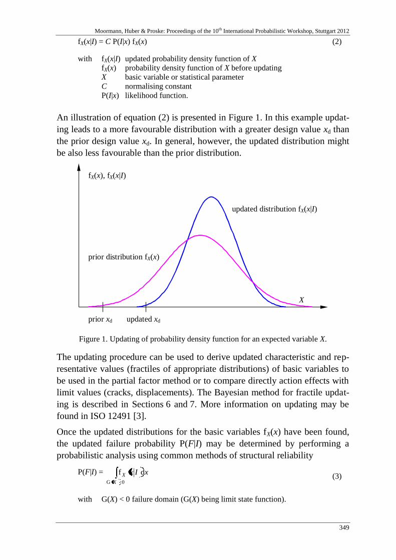
Moormann, Huber & Proske: Proceedings of the 10th International Probabilistic Workshop, Stuttgart 2012
349
fX(x|I) = C P(I|x) fX(x) (2)
with fX(x|I) updated probability density function of X
fX(x) probability density function of X before updating
X basic variable or statistical parameter
C normalising constant
P(I|x) likelihood function.
An illustration of equation (2) is presented in Figure 1. In this example updat-
ing leads to a more favourable distribution with a greater design value xd than
the prior design value xd. In general, however, the updated distribution might
be also less favourable than the prior distribution.
fX(x), fX(x|I)
X
prior distribution fX(x)
updated distribution fX(x|I)
updated xdprior xd
Figure 1. Updating of probability density function for an expected variable X.
The updating procedure can be used to derive updated characteristic and rep-
resentative values (fractiles of appropriate distributions) of basic variables to
be used in the partial factor method or to compare directly action effects with
limit values (cracks, displacements). The Bayesian method for fractile updat-
ing is described in Sections 6 and 7. More information on updating may be
found in ISO 12491 [3].
Once the updated distributions for the basic variables fX(x) have been found,
the updated failure probability P(F|I) may be determined by performing a
probabilistic analysis using common methods of structural reliability
P(F|I) =
0G
df
X
X xIx (3)
with G(X) < 0 failure domain (G(X) being limit state function).

Holicky & Sykora: Probabilistic assessment of existing structures
350
It should be proved that the probability P(F|I), given the design values for its
basic variables, does not exceed a specified target value.
4 Probability updating of a steel beam
This example of probability updating is adopted from [4,5]. Consider the limit
state function G(X), where X is a vector of basic variables, and the failure F is
described by the inequality G(X) < 0. If the result of an inspection of the
structure I is an event described by the inequality H > 0 then using equa-
tion (1) the updated probability of failure P(F| I) may be written as
P(F| I) = P(G(X) < 0| H > 0) = P(G(X) < 0 ∩ H > 0) / P(H > 0) (4)
For example consider a simply supported steel beam of the span L exposed to
permanent uniform load g and variable load q. The beam has the plastic sec-
tion modulus W and the steel strength fy.
Using the partial factor method the design condition Rd Sd > 0 between the
design value Rd of the resistance R and design value Sd of the load effect S
may be written as
W fyk / M - ( G gkL2/8 + Q qkL
2/8) > 0 (5)
with fyk characteristic yield strength
gk characteristic (nominal) value of permanent load g
qk characteristic (nominal) value of permanent load q
M, G, Q partial factors of steel, permanent and variable
load.
By analogy to equation (5) the limit state function G(X) follows as
G(X) = R - S = W fy - (gL2/8 + qL
2/8) (6)
where all the basic variables are generally considered as random variables de-
scribed by appropriate probabilistic models.
To verify its reliability the beam has been investigated and a proof loading up
to the level qtest is carried out. It is assumed that gact is the actual value of the
permanent load g. If the beam resistance is sufficient the information I ob-
tained is described as
I = {H > 0} = {W fy - (gact L2/8 + qtest L
2/8) > 0} (7)
with fy actual steel strength
gact actual permanent load determined reasonably accu-
rately using non-destructive methods.
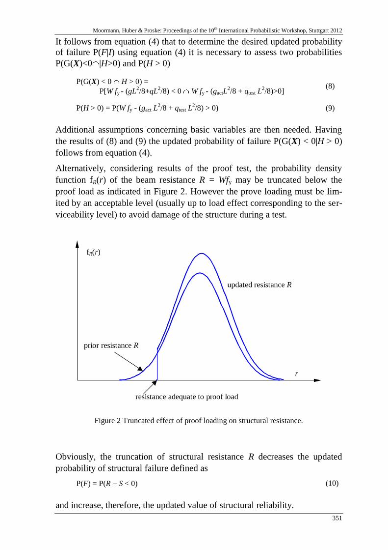
Moormann, Huber & Proske: Proceedings of the 10th International Probabilistic Workshop, Stuttgart 2012
351
It follows from equation (4) that to determine the desired updated probability
of failure P(F|I) using equation (4) it is necessary to assess two probabilities
P(G(X)<0 |H>0) and P(H > 0)
P(G(X) < 0 H > 0) =
P[W fy - (gL2/8+qL
2/8) < 0 W fy - (gactL
2/8 + qtest L
2/8)>0]
(8)
P(H > 0) = P(W fy - (gact L2/8 + qtest L
2/8) > 0) (9)
Additional assumptions concerning basic variables are then needed. Having
the results of (8) and (9) the updated probability of failure P(G(X) < 0|H > 0)
follows from equation (4).
Alternatively, considering results of the proof test, the probability density
function fR(r) of the beam resistance R = Wfy may be truncated below the
proof load as indicated in Figure 2. However the prove loading must be lim-
ited by an acceptable level (usually up to load effect corresponding to the ser-
viceability level) to avoid damage of the structure during a test.
fR(r)
r
updated resistance R
prior resistance R
resistance adequate to proof load
Figure 2 Truncated effect of proof loading on structural resistance.
Obviously, the truncation of structural resistance R decreases the updated
probability of structural failure defined as
P(F) = P(R S < 0) (10)
and increase, therefore, the updated value of structural reliability.
Holicky & Sykora: Probabilistic assessment of existing structures
352
5 Updating design values of basic variables
A more practical procedure is to determine updated design values for each
basic variable (procedure (2)). For a resistance parameter X, the design value
xd can be obtained using operational formula given in ISO 2394 [1], ISO
12491 [3] and study [6]. For normal and lognormal random variable it holds
xd = (1 - V)
xd = exp[- √(ln(1 + V2)) – 0.5 ln(1 + V
2)]
(11)
(12)
with xd updated design value of X
updated mean value
FORM sensitivity factor
target reliability index
V updated coefficient of variation of X.
Note that 2ln(1 )V V is equal to the standard deviation of the transformed
variable ln(X).
The value of the target reliability index is discussed by Holicky and Retief
[7], the sensitivity factors can be taken equal to those commonly used for
new structures (the values −0.7 for the dominating load parameter, +0.8 for
the dominating resistance parameter and the reduced values to 40 % for non-
dominating variables are recommended in ISO 2394 [1]).
As an alternative to procedure (2), one might also determine the characteristic
value xk first and calculate the design value xd by applying the appropriate
partial factor m
xd = xk / m (13)
For normal and lognormal random variable X the characteristic value xk are
xk = (1 - k V)
xd = exp[-k √(ln(1 + V2)) – 0.5 ln(1 + V
2)]
(14)
(15)
with k = 1.645 (5% fractile of the standardised normal distribu-
tion) usually applied for the characteristic strength.
This procedure may be applied for all basic variables. However, for geomet-
rical properties and variable loads also other distributions (in addition to the
normal and lognormal distribution) are frequently applied.
Note that a lower acceptable reliability level can be specified by reducing
- values for probabilistic design and reducing - values in the partial factor
method. For a material property X described by a normal or lognormal distri-
bution the partial factor m = xk / xd may be estimated using equation
Moormann, Huber & Proske: Proceedings of the 10th International Probabilistic Workshop, Stuttgart 2012
353
m = (1 - k V) / (1 - V), or m = exp[(-k + )√(ln(1 + V2))] (16)
which follows from general equations (11) to (15). All the symbols used in
(16) are defined above. The second expression in (16) for m is valid for the
lognormal distribution; similar expressions may be derived for other distribu-
tions.
6 Bayesian fractile updating
Fractiles of basic variables can be effectively updated using the Bayesian ap-
proach described in ISO 12491 [3]. This procedure is limited here to a normal
variable X only for which the prior distribution function ( ) of and is
given as
2 21
2
1, exp
2
nC s n m (17)
with C normalising constant
(n') = 0 for n' = 0 and (n') = 1 otherwise.
The prior parameters m', s', n', ' are parameters asymptotically given as
E( ) = m', E( ) = s', V( ) =s
m n, V
1
2 (18)
while the parameters n' and ' are independent and may be chosen arbitrarily
(it does not hold that ' = n' – 1). In equation (18) E(∙) denotes the expectation
and V(∙) the coefficient of variation of the variable in brackets. Equations (18)
may be used to estimate unknown parameters n' and ' provided the values
V( ) and V( ) are estimated using experimental data or available experience.
The posterior distribution function "( , ) of and is of the same type as
the prior distribution function, but with parameters m", s", n" and ", given as
n" = n' + n
" = ' + + ( n )
m"n"= n'm' + nm
"(s")2 + n"(m")
2 = '(s')
2 + n'(m')
2 + s
2 + nm
2.
(19)
with m sample mean
s sample standard deviation
n size of the observed sample
= n – 1 number of degrees of freedom.
The predictive value xp,pred of a fractile xp is then
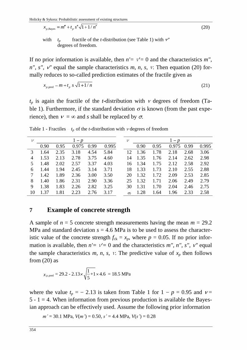
Holicky & Sykora: Probabilistic assessment of existing structures
354
,B 1 1/p ayes px m t s n (20)
with tp fractile of the t-distribution (see Table 1) with "
degrees of freedom.
If no prior information is available, then n'= '= 0 and the characteristics m",
n", s", " equal the sample characteristics m, n, s, . Then equation (20) for-
mally reduces to so-called prediction estimates of the fractile given as
,pred 1 1/p px m t s n (21)
tp is again the fractile of the t-distribution with degrees of freedom (Ta-
ble 1). Furthermore, if the standard deviation is known (from the past expe-
rience), then = and s shall be replaced by .
Table 1 - Fractiles tp of the t-distribution with degrees of freedom
1 p 1 p
0.90 0.95 0.975 0.99 0.995 0.90 0.95 0.975 0.99 0.995
3
4
5
6
7
8
9
10
1.64
1.53
1.48
1.44
1.42
1.40
1.38
1.37
2.35
2.13
2.02
1.94
1.89
1.86
1.83
1.81
3.18
2.78
2.57
2.45
2.36
2.31
2.26
2.23
4.54
3.75
3.37
3.14
3.00
2.90
2.82
2.76
5.84
4.60
4.03
3.71
3.50
3.36
3.25
3.17
12
14
16
18
20
25
30
1.36
1.35
1.34
1.33
1.32
1.32
1.31
1.28
1.78
1.76
1.75
1.73
1.72
1.71
1.70
1.64
2.18
2.14
2.12
2.10
2.09
2.06
2.04
1.96
2.68
2.62
2.58
2.55
2.53
2.49
2.46
2.33
3.06
2.98
2.92
2.88
2.85
2.79
2.75
2.58
7 Example of concrete strength
A sample of n = 5 concrete strength measurements having the mean m = 29.2
MPa and standard deviation s = 4.6 MPa is to be used to assess the character-
istic value of the concrete strength fck = xp, where p = 0.05. If no prior infor-
mation is available, then n'= '= 0 and the characteristics m", n", s", " equal
the sample characteristics m, n, s, . The predictive value of xp then follows
from (20) as
pred
1 = 29.2 - 2.13 +1 4.6 = 18.5 MPa
5p, x
where the value tp = 2.13 is taken from Table 1 for 1 p = 0.95 and =
5 - 1 = 4. When information from previous production is available the Bayes-
ian approach can be effectively used. Assume the following prior information
m’ = 30.1 MPa, V(m’) = 0.50, s’ = 4.4 MPa, V(s’) = 0.28
Moormann, Huber & Proske: Proceedings of the 10th International Probabilistic Workshop, Stuttgart 2012
355
It follows from equation (18)
24.6 1
= < 130.1 0.50
n , 2
1 1 = 6
2 0.28
The following characteristics are therefore considered: n' = 0 and ' = 6. Tak-
ing into account that = n - 1 = 4, equations (19) yield
= 5, = 10, = 29.2 MPa, = 4.5 MPan m s
and finally it follows from equation (20)
Bayes
1 = 29.2 - 1,81 +1 4.5 = 20.3 MPa
5p, x
where the value tp = 1.81 is taken from Table 1 for 1 p = 0.95 and = 10.
In this example the resulting characteristic strength is greater (by about 10 %)
than the value obtained by prediction method without using prior information.
Thus, when previous information is available the Bayesian approach may im-
prove (not always) the fractile estimate, particularly in the case of a great var-
iance of the variable. In any case due caution should be paid to the origin of
the prior information with regard to the nature of considered variable.
8 Concluding remarks
The main principles of the assessment of existing structures are:
- Currently valid codes for verification of structural reliability should be ap-
plied, historic codes valid in the period when the structure was designed,
should be used only as guidance documents;
- Actual characteristics of structural material, action, geometric data and
structural behaviour should be considered; the original design documentation
including drawing should be used as guidance material only.
Typically, the assessment of existing structures is a cyclic process in which
the first preliminary assessment is often supplemented by subsequent detailed
investigations and assessment. A report on structural assessment prepared by
an engineer should include a recommendation on possible intervention. How-
ever, the client in collaboration with the relevant authority should make the
final decision concerning possible interventions.
The assessment of existing structures often requires application of sophisti-
cated probabilistic methods, as a rule beyond the scope of traditional design
practice. The critical step of the probabilistic assessment itself is specification
Holicky & Sykora: Probabilistic assessment of existing structures
356
of the target reliability level discussed already during the previous Interna-
tional Probabilistic Workshop in Braunschweig. The other important steps of
the whole assessment include evaluation of inspection data and updating of
prior information concerning strength and structural reliability. It appears that
a Bayesian approach can provide an effective tool. Described methods of
probability updating are frequently used in assessment of existing structures.
Two types of probability updating are generally applied:
(1) Updating of the structural failure probability.
(2) Updating of the probability distributions of basic variables.
The second type of updating seems to be more operational and effective. It
enables to determine directly the design values of basic variables or updated
partial factors that can be subsequently used in structural assessment.
9 Acknowledgements
This study project has been conducted within the project CZ/11/LLP-
LdV/TOI/134005 Vocational Training in Assessment of Existing Structures,
funded with support from the European Commission (programme Leonardo
da Vinci). The paper reflects views only of the authors, and the Commission
cannot be held responsible for any use which may be made of the information
contained therein. Results of the project LG11043 have been utilised.
10 Literature
[1] ISO 2394: General principles on reliability of structures, 1998.
[2] ISO 13822: Basis for design of structures -Assessment of existing structures, 2008.
[3] ISO 12491: Statistical methods for quality control of building materials and compo-
nents, 1998.
[4] Melchers R.E.: Structural reliability analysis and prediction. Wiley & Sons, 2001.
[5] Ellingwood B.R.: Reliability-based condition assessment and LRFD for existing
structures. Structural Safety, 18 (2+3), 1996, 67-80.
[6] Holický M.: Assessment of existing structures. Chapter 9 of Structural Safety and Its
Quality Assurance. Edited by B.R. Ellingwood and Jun Kanda. ASCE, 2005.
[7] Holický M., Retief J.: Theoretical Basis of the Target Reliability, IPW, Braun-
schweig, 2011, 91-101.
Moormann, Huber & Proske: Proceedings of the 10th International Probabilistic Workshop, Stuttgart 2012
357
Stochastic material properties for different
concrete types: An experimental investigation
Thomas Zimmermann, Katharina Haider & Alfred Strauss
Institute for Structural Engineering, University of Natural Resources and Life
Sciences, Vienna, Austria
Abstract: Within this paper an experimental investigation on basic material
parameters as well as fracture mechanical properties for different concrete
types is presented. In total four different concrete types – C30/37 H,
C25/30 B3, C25/30 XC1 GK16 and C20/25 XC1 GK16 – were investigated.
The results of this investigation serve as a basis for further numerical assess-
ment with respect to (a) define suitable stochastic models and (b) to carry out
non-linear finite element analysis. An additional target was to capture the ef-
fects of testing procedure on the mechanical properties. The associated
knowledge of these material parameters is an important issue for a realistic re-
liability assessment of both new as well as existing structures.
1 Introduction
Design, computation and construction of engineering structures are generally
based on linear static analyses and on linear or multi-linear material models.
In the new generation of design specifications, dispersion effects and associ-
ated uncertainties, e.g. in material properties, are covered in the so-called
semi-probabilistic safety concept (SPSC) [3]. The SPSC guarantees desired
reliability levels over the life-cycle of a structure by careful selection of (a)
suitable safety factors for the resistance and for the action side, and of (b) load
combination factors.
The SPSC provides for particular structures, using fractiles of material prop-
erties and loads as inputs, the means for a standardized verification of the us-
ability and the static safety of the structures. The demanded general validity
of the SPSC for a wide range of structure types gives rise to reliability levels
that may turn out to be even higher than originally intended [13].
Zimmermann, Haider & Strauss: Stochastic material properties for different concrete types: An experimental investiga-
tion
358
Moreover an accurate knowledge concerning the material behaviour and the
available capacity of a structure can be used for further life-cycle analysis. In
particular, optimized strategies and concepts for maintenance and revitaliza-
tion over the life-time of a structure can be developed. If therefore also differ-
ent cost factors are taken into account a valuation concept and decision
concept for immediate and necessary future actions can be created. Investiga-
tions for different engineering structure can be found e.g. in [5] and [14].
However the knowledge of the scattering quantities and suitable stochastic
models are necessary.
The determination of the statistics and probability distributions of the random
variables describing material properties play an important role in the devel-
opment of probabilistic based design specifications. The choice of the proba-
bility distribution chosen to represent the material property data will have a
large effect on the calculated reliability. Assuming different distributions for
the material properties can result in computed probabilities of failure that vary
by over an order of magnitude. This is the result of the lower tail behaviour of
different cumulative distribution functions, which has become known as the
tail-sensitivity problem in structural reliability [2].
2 Laboratory tests
2.1 Materials and test setup
In general, the properties of concrete are characterized based on the compres-
sive strengths according to EN 206-1, on the exposure classes and on the
slump value. Nevertheless, the realistic modelling of structures requires the
incorporation of (a) nonlinear effects in the analysis and material properties,
which can be captured for e.g., concrete by a variable modulus of elasticity,
Ec the compressive strength, fc and the fracture energy, Gf, and of (b) uncer-
tainties in material and geometrical properties caused by nature, manufactur-
ing processes and curing among others. These requirements, together with the
newly characterized concrete classes in the Eurocode concept, forces the in-
terest in experimental investigations with commonly used concrete types, e.g.
C25/30 according to EN 206-1 or Önorm B 4710-1_ENREF_17.
In particular, the standardized compressive test and the wedge splitting test
were accomplished. These investigations were divided into four parts: (I)
concrete C30/37 H, (II) concrete C25/30 B3, (III) concrete C25/30 XC1 and
(IV) concrete C20/25 XC1. Table 1 shows the mixture for these different con-
crete types.
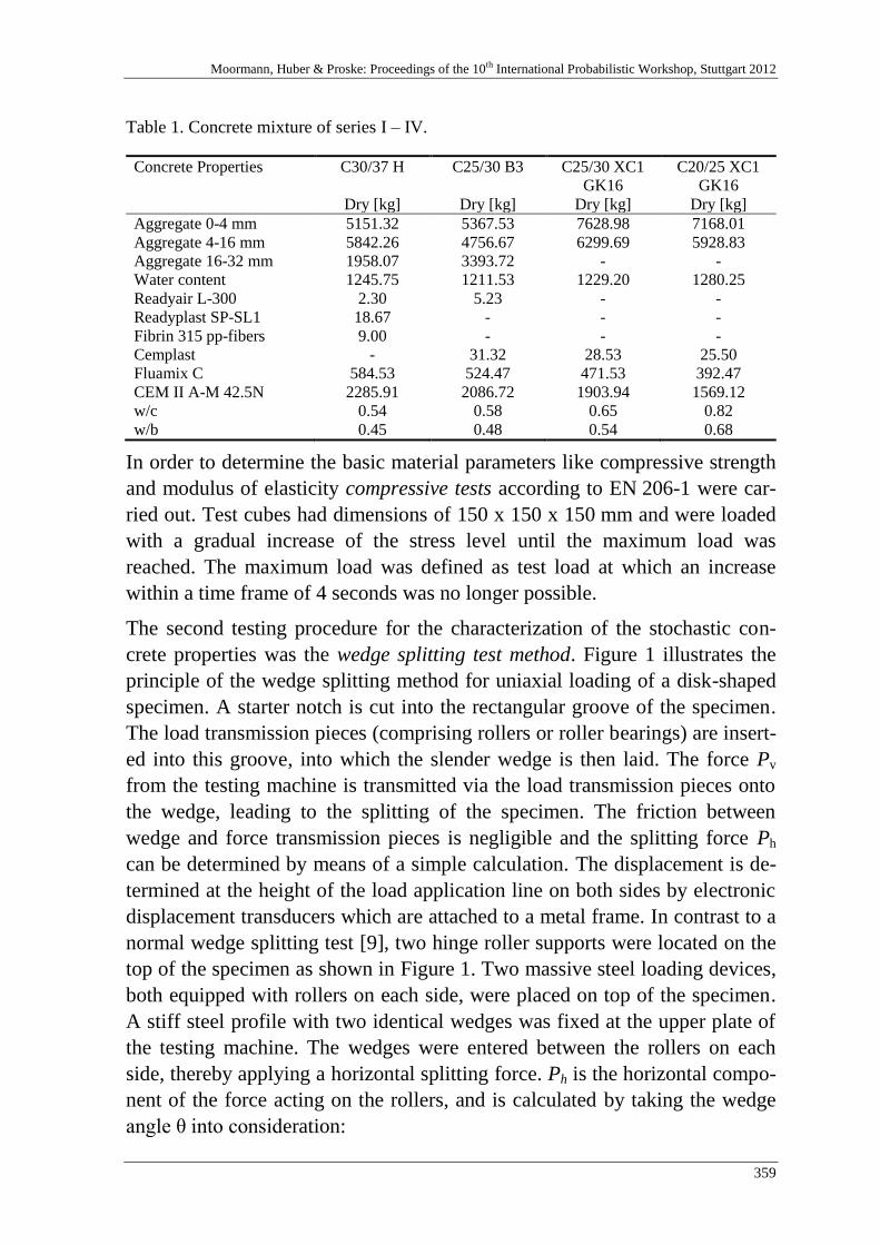
Moormann, Huber & Proske: Proceedings of the 10th International Probabilistic Workshop, Stuttgart 2012
359
Table 1. Concrete mixture of series I – IV.
Concrete Properties C30/37 H C25/30 B3 C25/30 XC1
GK16
C20/25 XC1
GK16
Dry [kg] Dry [kg] Dry [kg] Dry [kg]
Aggregate 0-4 mm 5151.32 5367.53 7628.98 7168.01
Aggregate 4-16 mm 5842.26 4756.67 6299.69 5928.83
Aggregate 16-32 mm 1958.07 3393.72 - -
Water content 1245.75 1211.53 1229.20 1280.25
Readyair L-300 2.30 5.23 - -
Readyplast SP-SL1 18.67 - - -
Fibrin 315 pp-fibers 9.00 - - -
Cemplast - 31.32 28.53 25.50
Fluamix C 584.53 524.47 471.53 392.47
CEM II A-M 42.5N 2285.91 2086.72 1903.94 1569.12
w/c 0.54 0.58 0.65 0.82
w/b 0.45 0.48 0.54 0.68
In order to determine the basic material parameters like compressive strength
and modulus of elasticity compressive tests according to EN 206-1 were car-
ried out. Test cubes had dimensions of 150 x 150 x 150 mm and were loaded
with a gradual increase of the stress level until the maximum load was
reached. The maximum load was defined as test load at which an increase
within a time frame of 4 seconds was no longer possible.
The second testing procedure for the characterization of the stochastic con-
crete properties was the wedge splitting test method. Figure 1 illustrates the
principle of the wedge splitting method for uniaxial loading of a disk-shaped
specimen. A starter notch is cut into the rectangular groove of the specimen.
The load transmission pieces (comprising rollers or roller bearings) are insert-
ed into this groove, into which the slender wedge is then laid. The force Pv
from the testing machine is transmitted via the load transmission pieces onto
the wedge, leading to the splitting of the specimen. The friction between
wedge and force transmission pieces is negligible and the splitting force Ph
can be determined by means of a simple calculation. The displacement is de-
termined at the height of the load application line on both sides by electronic
displacement transducers which are attached to a metal frame. In contrast to a
normal wedge splitting test [9], two hinge roller supports were located on the
top of the specimen as shown in Figure 1. Two massive steel loading devices,
both equipped with rollers on each side, were placed on top of the specimen.
A stiff steel profile with two identical wedges was fixed at the upper plate of
the testing machine. The wedges were entered between the rollers on each
side, thereby applying a horizontal splitting force. Ph is the horizontal compo-
nent of the force acting on the rollers, and is calculated by taking the wedge
angle θ into consideration:
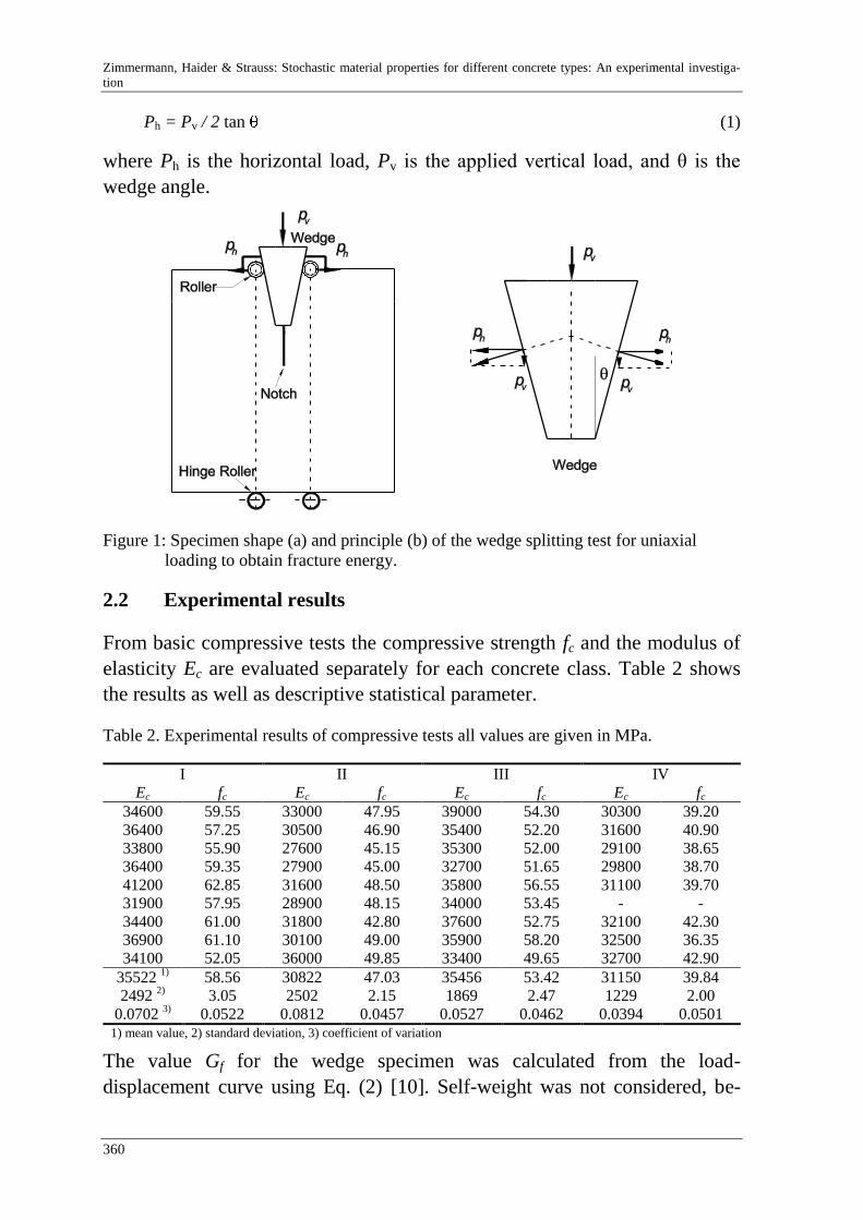
Zimmermann, Haider & Strauss: Stochastic material properties for different concrete types: An experimental investiga-
tion
360
Ph = Pv / 2 tan (1)
where Ph is the horizontal load, Pv is the applied vertical load, and θ is the
wedge angle.
Figure 1: Specimen shape (a) and principle (b) of the wedge splitting test for uniaxial
loading to obtain fracture energy.
2.2 Experimental results
From basic compressive tests the compressive strength fc and the modulus of
elasticity Ec are evaluated separately for each concrete class. Table 2 shows
the results as well as descriptive statistical parameter.
Table 2. Experimental results of compressive tests all values are given in MPa.
I II III IV
Ec fc Ec fc Ec fc Ec fc
34600 59.55 33000 47.95 39000 54.30 30300 39.20
36400 57.25 30500 46.90 35400 52.20 31600 40.90
33800 55.90 27600 45.15 35300 52.00 29100 38.65
36400 59.35 27900 45.00 32700 51.65 29800 38.70
41200 62.85 31600 48.50 35800 56.55 31100 39.70
31900 57.95 28900 48.15 34000 53.45 - -
34400 61.00 31800 42.80 37600 52.75 32100 42.30
36900 61.10 30100 49.00 35900 58.20 32500 36.35
34100 52.05 36000 49.85 33400 49.65 32700 42.90
35522 1)
58.56 30822 47.03 35456 53.42 31150 39.84
2492 2)
3.05 2502 2.15 1869 2.47 1229 2.00
0.0702 3)
0.0522 0.0812 0.0457 0.0527 0.0462 0.0394 0.0501 1) mean value, 2) standard deviation, 3) coefficient of variation
The value Gf for the wedge specimen was calculated from the load-
displacement curve using Eq. (2) [10]. Self-weight was not considered, be-
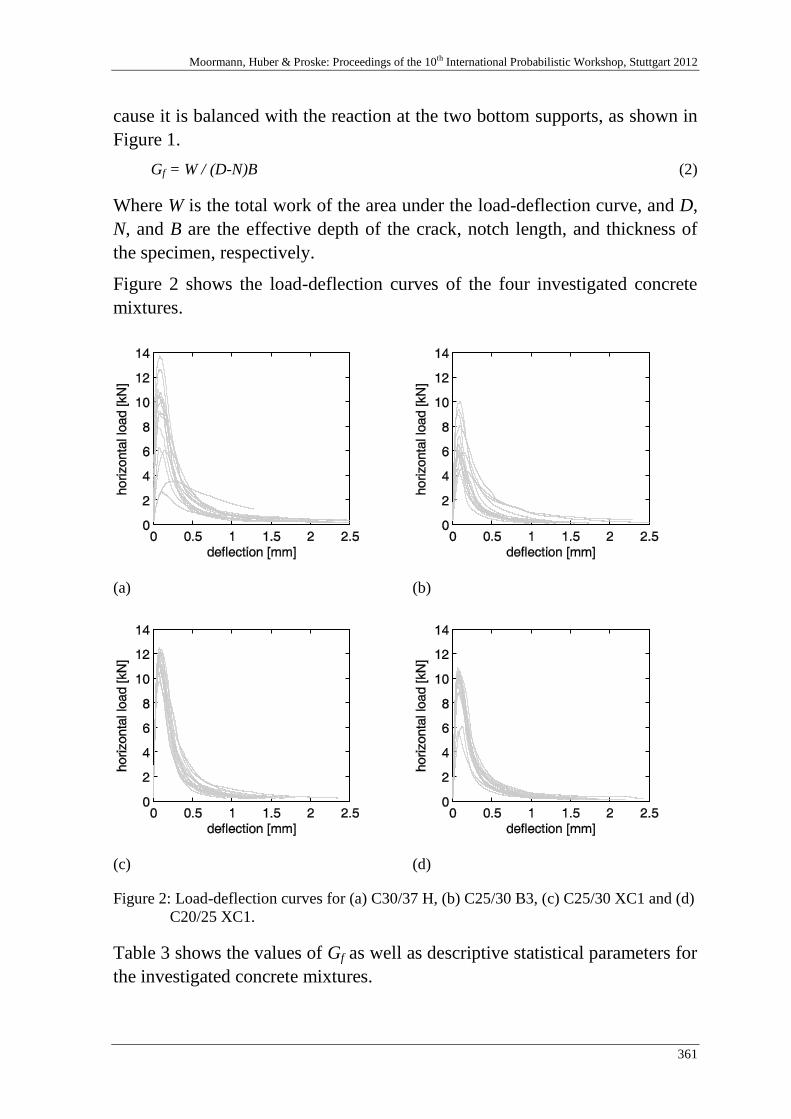
Moormann, Huber & Proske: Proceedings of the 10th International Probabilistic Workshop, Stuttgart 2012
361
cause it is balanced with the reaction at the two bottom supports, as shown in
Figure 1.
Gf = W / (D-N)B (2)
Where W is the total work of the area under the load-deflection curve, and D,
N, and B are the effective depth of the crack, notch length, and thickness of
the specimen, respectively.
Figure 2 shows the load-deflection curves of the four investigated concrete
mixtures.
(a) (b)
(c) (d)
Figure 2: Load-deflection curves for (a) C30/37 H, (b) C25/30 B3, (c) C25/30 XC1 and (d)
C20/25 XC1.
Table 3 shows the values of Gf as well as descriptive statistical parameters for
the investigated concrete mixtures.
Zimmermann, Haider & Strauss: Stochastic material properties for different concrete types: An experimental investiga-
tion
362
Table 3. Experimental results of wedge splitting tests all values are given in N/m.
I II III IV
223.7 223.7 183.3 163.7
189.0 189.0 167.9 135.0
185.4 185.4 187.9 163.9
207.9 207.9 179.3 120.3
173.9 173.9 201.4 137.2
165.7 165.7 179.6 -
203.6 203.6 190.2 124.6
123.3 - 172.0 153.8
161.8 161.8 188.2 171.4
181.6 1)
188.9 183.3 146.2
28.13 2)
20.30 9.52 18.22
0.1549 3)
0.1075 0.0519 0.1246 1) mean value, 2) standard deviation, 3) coefficient of variation
3 Probabilistic models
Depending on the distribution function different procedures for the estimation
of the unknown parameters have been used e.g. Method of Moments and
Method of Maximum Likelihood. However choosing of the best fitted model
to a given dataset was based on Kolmogorov Smirnov (KS) [1]. The fitting of
suitable probability density functions to the obtained data set was done by us-
ing program FReET [6], [7].
Table 4. Recommended values of statistics and distribution functions.
item pdf mean
[MPa]
std
[MPa]
cov skew-
ness
excess
Ec I Weibull max 35522 2643.3 0.07441 0.92819 1488
Ec II Weibull max 30822 2654.1 0.08611 0.60009 0.47757
Ec III Lognormal 35456 1982.5 0.05592 0.37134 0.24615
Ec IV Weibull max 31150 1313.7 0.04217 -0.30699 -0.18949
fc I Weibull min 58.556 32.395 0.05532 -0.72044 0.79474
fc II Weibull min 47.033 2.282 0.04852 -0.92431 14732
fc III Weibull max 53.417 26.153 0.04896 0.57068 0.40901
fc IV Lognormal 39.838 21.335 0.05356 0.16082 0.04602
Gf I Weibull max 181.59 29.834 0.16429 -0.53046 0.07344
Gf II Weibull max 188.88 21.706 0.11492 0.24819 -0.12609
Gf III Normal 183.31 10.093 0.05506 0 0
Gf IV Weibull max 146.24 19.479 0.13320 -0.05244 -0.28935
As a result of the fitting process the data set can be represented in most cases
by a Weibull distribution function. Using Weibull max or min is depending on
the skewness of data. However in some cases also Lognormal or Normal dis-
tribution is a suitable distribution function to represent the experimentally ob-
Moormann, Huber & Proske: Proceedings of the 10th International Probabilistic Workshop, Stuttgart 2012
363
tained data. It should be also taken into account that the accuracy of the fitting
process is highly influenced by the number of samples, especially if probabil-
ity density functions with more than two parameters are used.
4 Reliability assessment
In general, two basic analytical methods, FORM and SORM, can be used to
estimate structural reliability [1]. Furthermore, numerical approximation
techniques such as the Response Surface Method or Monte Carlo Sampling
are available. It was verified that FORM reliability analyses provides in many
cases an excellent approximation, even for nonlinear conditions. The design
of any structure requires that its resistance R is greater than the load effect Q.
This requirement (i.e., R > Q) is described by the limit state
g(X) = R – Q = 0 (3)
where X = {X1, X2, …, Xn}T = vector of random variables, g(X) = 0 = limit
state, and g(X) < 0 is the failure region. The reliability index then is defined
as
ß = (µR – µQ) / (2
R + 2Q)
1/2 (4)
where µR and µQ = mean resistance and mean load effect, respectively, and R
and Q = standard deviations of both variables. If the resistance R and the load
effect Q are normally distributed, g(X) is normally distributed too and the
probability of failure pf can be determined as
pf = Ф(-ß) (5)
where Ф = standard normal distribution. The calculation of the reliability in-
dex ß is a constrained optimization problem, where the closest point of the
limit state surface with regard to the origin is searched in the standard normal
space [12].
5 Conclusions
In order to determine experimentally the basic material parameters was well
as fracture mechanical properties for different concrete types, four concrete
types (C 30/37 H, C 25/30 B3, C25/30 XC1 GK16 and C20/25 XC1 GK16)
were investigated.
The basic material parameters like compressive strength and modulus of elas-
ticity were assigned by compressive tests according to EN 206-1. For the
Zimmermann, Haider & Strauss: Stochastic material properties for different concrete types: An experimental investiga-
tion
364
characterization of the stochastic concrete properties for non-linear modelling
purposes the wedge splitting test method was used.
After the laboratory tests the compressive strength fc and the modulus of elas-
ticity Ec were evaluated separately for each concrete class. Within this inves-
tigation the mean value, the standard deviation as well as the coefficient of
variation was calculated.
With respect to the wedge-splitting tests for all investigated concrete mixtures
the load-deflection curve was figured out and the descriptive statistical pa-
rameters out of the test results were calculated as well.
Afterwards, suitable probability density functions were fitted to the obtained
data-set of the obtained material parameters by using program FReET. The
best fitted probabilistic model was chosen by using the Kolmogorov Smirnov
test.
Obtained data as well as fitted probabilistic models can serve as a basis for a
further reliability assessment to calculate reliability index β and probability of
failure pf respectively.
6 Acknowledgement
The support of the experimental investigations by the project
CZ.1.07/2.3.00/30.0005 of Brno University of Technology is gratefully
acknowledged.
7 References
[1] Ang, A.H.-S.; Tang, W.H.: Probability Concepts in Engineering. John Wiley &
Sons, Inc. 2007
[2] Ditlevsen, O.: Uncertainty Modeling with Applications to Multidimensional Civil
Engineering Systems. McGraw-Hill International Book Co. New York, London,
1981
[3] Ellingwood, B.R.: Structural Reliability and Performance-Based Engineering,
Proceedings of the Institution of Civil Engineers: Structures and Buildings, 161, 199-
207, 2008
[4] EN 206-1 Concrete – Part 1: Specification, Performance, Production and Conformity
CEN/TC 104.
[5] Frangopol, D.M.; Strauss, A.; Bergmeister, K.: Lifetime cost optimization of struc-
tures by a combined condition-reliability approach, Engineering Structures, 31(7):
1572-1580, 2009

Moormann, Huber & Proske: Proceedings of the 10th International Probabilistic Workshop, Stuttgart 2012
365
[6] Novák, D.; Vořechovský, M.; Rusina, R.: FReET v.1.6 – program documentation.
User´s and Theory Guides. Červenka Consulting, Czech Republic,
http://www.freet.cz, 2011
[7] Novák, D.; Pukl, R.: Simulation of random behavior of engineering structures: From
parameters identification to reliability assessment. Proceedings of the 3rd Interna-
tional Symposium on Life-Cycle Civil Engineering, IALCCE 2012
[8] ÖNORM B 4710-1 – Part 1: Festlegung, Herstellung, Verwendung und
Konformitätsnachweis. 2003
[9] Petersson, P.E.: Fracture Energy of Concrete: Practical Performance and Experi-
mental Results, Cement and Concrete Research, V.10, No.1, pp.91-101, 1980
[10] Rossi, P.; Brühwiler, E.; Chhuy, S.; Jenq, Y.S.; Shah, S. P, “Fracture Properties of
Concrete as Determined by Means of Wedge Splitting Tests and Tapered Double
Cantilever Beam Tests, ” in: S. P. Shah, A. Carpentari (Eds.),Chapman & Hall, Lon-
don, pp. 87-126. 1990
[11] Schneider, J.: Sicherheit und Zuverlässigkeit im Bauwesen – Grundwissen für Inge-
nieure. Stuttgart, Teubner, 1996
[12] Shinozuka, M.: Basic Analysis of Structural Safety. Journal of Structural Engineer-
ing 1109(3): 721-740, 1983
[13] Strauss, A.; Bergmeister, K.; Hoffmann, S.; Pukl, R.; Novak, D.: Advanced Life-
Cycle Analysis of Existing Concrete Bridges, Journal of Materials in Civil
Engineering, 20, 9-19, 2008
[14] Strauss, A.; Frangopol, D.M.; Bergmeister, K.: Assessment of Existing Structures
Based on Identification, Journal of Structural Engineernig, ASCE, 136(1): 86-97,
2010

Zimmermann, Haider & Strauss: Stochastic material properties for different concrete types: An experimental investiga-
tion
366

Moormann, Huber & Proske: Proceedings of the 10th International Probabilistic Workshop, Stuttgart 2012
367
Development of a finite element model for ma-
sonry arch bridges incorporating stochastic
material parameters
Alexander Krawtschuk, Thomas Zimmermann, Katharina Haider,
Alfred Strauss & Oliver Zeman
Institute of Structural Engineering, University of Natural Resources and Life
Sciences, Vienna
Abstract: Due to the fact that historical arch bridges nowadays are one of the
oldest infrastructural buildings which are still in usage, the estimation of the
bearing capacity of these structures is quite important to companies responsible
for maintenance. In most cases the material parameters and the geometrical
shape are unknown which leads to an uncertainty in the determination of the
bearing behaviour. Therefore, this contribution focuses on the development of
a finite element model which aims for the detection of the most unfavourable
geometrical form of a masonry arch bridge, which is presented in this contribu-
tion by means of a sensitivity analysis of a few arch shapes (circular, three-
centre and parabolic shaped). As a second part, the contribution discusses the
procedure of the calibration of an appropriate finite element model for further
assessments. In addition the experimental program to determine the input pa-
rameters as well as to quantify stochastic properties is pointed out. By means of
these stochastic material parameters the accuracy of the finite element model
can be increased for a realistic and useable approach on existing historical arch
bridges.
1 Introduction
Arch bridges made from nature stone nowadays are the oldest structures which are still in
use on road and railway lines. With an average age of more than hundred years, these
structures often are seen as historical important buildings. Most of them had been con-
Krawtschuk, Zimmermann, Haider, Strauss & Zeman: Development of a finite element model for masonry arch bridges
incorporating stochastic material parameters
368
structed during the great building period of roads and railways from the 1840ies to 1900.
Lots of the considered nature stone bridges are constructed as circle or three centre curve,
some of them also in a parabolic form or catenaries or cycloid. The height of the apex cov-
er varies in a large range. When masonry was appropriated, usually sand, chalkstone or
clay bricks were used. For most bridges no observations of the material parameter are
available, as a result the stone and the mortar strengths are unknown. Under the usage of
the German railway company, there are more than 8000 arch bridges yet, although at local
roads there is an additional unknown number of them. In Austria, the railway network,
especially along the southern railway line has around 1000 arch bridges in usage. In whole
Europe, the stock of masonry railway bridges is estimated with around 70.000. In the
course of route expansion plans in the past especially arch bridges have been replaced by
new steel or reinforced concrete structures. Considerations of preservation, the budgetary
situation of the rail and road operators, as well as a sustainable, efficient usage of resources
and existing infrastructure are motivations to maintain and – if necessary – toughen up
existing arch bridges. Therefore, the issues of sustainability, durability and serviceability
become more important [4].
2 State of the art
The oldest existing arch bridges were designed based on experience. Later graphical meth-
ods for the static were available and approximation formulas based on the arch thrust line
to design major geometrical parameters such as span, arch shape and arch thickness at the
apex and the abutments were developed. These simplifying estimations can also now be
useful to perform the bearing capacity of existing arch bridges on the basis of their geomet-
rical parameters. Especially for old arch bridges which were designed for different loads at
their design and construction date, these methods can be used as an first estimation for the
current bearing capacity or the future use of these buildings. The recalculation of these
buildings under the valid load approach enables the assessment of the bearing capacity and
the suitability for an usage under nowadays valid load. Any necessary upgrading which
considers the conservation of the existing structures both preserves the appearance of the
arch bridges and saves costs. For the estimation of the bearing capacity as a result of a stat-
ic recalculation, the knowledge of the construction and the material properties is required.
If bridges are designed nowadays, e.g. made from reinforced concrete, steel or wood, these
parameters are well known. In case of existing arch bridges made from stone, brick or
rammed concrete, the material properties often cannot be identified, because too many fac-
tors influencing the bearing capacity [6].
The assessment of existing bridge structures can be used as a helpful method for the re-
sponsible organisations, e.g. road or railway maintenance companies, and the proper gov-
ernments. In terms of the life cycle concept, the increasing axle loads, load restrictions,
inspections, monitoring, maintenance measurements or even a replacement of the struc-
tures have to be considered. A conventional approach for the recalculation of arch bridges,
the elasticity theory can provide results which differ significantly from the actual bearing
capacity. The involvement of the wing walls and the interaction with the surrounding soil
influence the capacity significantly. Therefore the issue of structure-soil-interaction as de-
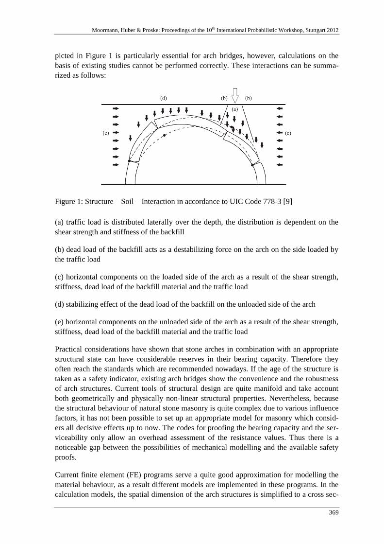
Moormann, Huber & Proske: Proceedings of the 10th International Probabilistic Workshop, Stuttgart 2012
369
picted in Figure 1 is particularly essential for arch bridges, however, calculations on the
basis of existing studies cannot be performed correctly. These interactions can be summa-
rized as follows:
Figure 1: Structure – Soil – Interaction in accordance to UIC Code 778-3 [9]
(a) traffic load is distributed laterally over the depth, the distribution is dependent on the
shear strength and stiffness of the backfill
(b) dead load of the backfill acts as a destabilizing force on the arch on the side loaded by
the traffic load
(c) horizontal components on the loaded side of the arch as a result of the shear strength,
stiffness, dead load of the backfill material and the traffic load
(d) stabilizing effect of the dead load of the backfill on the unloaded side of the arch
(e) horizontal components on the unloaded side of the arch as a result of the shear strength,
stiffness, dead load of the backfill material and the traffic load
Practical considerations have shown that stone arches in combination with an appropriate
structural state can have considerable reserves in their bearing capacity. Therefore they
often reach the standards which are recommended nowadays. If the age of the structure is
taken as a safety indicator, existing arch bridges show the convenience and the robustness
of arch structures. Current tools of structural design are quite manifold and take account
both geometrically and physically non-linear structural properties. Nevertheless, because
the structural behaviour of natural stone masonry is quite complex due to various influence
factors, it has not been possible to set up an appropriate model for masonry which consid-
ers all decisive effects up to now. The codes for proofing the bearing capacity and the ser-
viceability only allow an overhead assessment of the resistance values. Thus there is a
noticeable gap between the possibilities of mechanical modelling and the available safety
proofs.
Current finite element (FE) programs serve a quite good approximation for modelling the
material behaviour, as a result different models are implemented in these programs. In the
calculation models, the spatial dimension of the arch structures is simplified to a cross sec-

Krawtschuk, Zimmermann, Haider, Strauss & Zeman: Development of a finite element model for masonry arch bridges
incorporating stochastic material parameters
370
tion of one meter. The most important point for a correct modelling is to identify the rele-
vant meter-stripe and to describe the loadings correctly, particularly single loads in the
transversal direction of the arch.
The well-known graphical methods with thrust line have been followed by analytical
methods, particularly since the development of computational calculations. By means of
elasticity and plasticity theory, the models were enhanced, although there is still no satis-
factory solution approach for the issue of the discontinuous joint. Since a few years, some
FE-Programs can bear with discontinuous joints, but these models require an enormous
calculation effort. Additionally, there is the possibility that these models give completely
wrong results, as a result of unknown boundary conditions.
3 Motivation and Method
In order to develop an appropriate numerical model for the assessment of masonry arch
bridges the assessment procedure according to Figure 2 has been used. First of all in-situ
measurements on the real structure under defined loading situations were carried out. Sec-
ondly, based on a survey of the real structure a FE-model was set up. Another input for the
FE-model are results from laboratory tests in order to define the material properties. Af-
terwards the correlation between simulated (msi) and measured (mei) reactions is calculated.
If the accuracy between both values is in an appropriate state the FE-model is suitable for
further investigations (life-time assessment, decision-making tool etc.), otherwise an up-
date process has to be performed [8], [10].
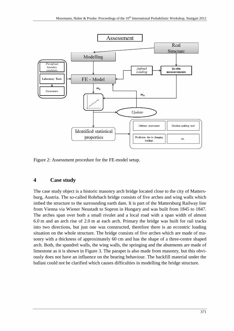
Moormann, Huber & Proske: Proceedings of the 10th International Probabilistic Workshop, Stuttgart 2012
371
Figure 2: Assessment procedure for the FE-model setup.
4 Case study
The case study object is a historic masonry arch bridge located close to the city of Matters-
burg, Austria. The so-called Rohrbach bridge consists of five arches and wing walls which
imbed the structure to the surrounding earth dam. It is part of the Mattersburg Railway line
from Vienna via Wiener Neustadt to Sopron in Hungary and was built from 1845 to 1847.
The arches span over both a small rivulet and a local road with a span width of almost
6.0 m and an arch rise of 2.0 m at each arch. Primary the bridge was built for rail tracks
into two directions, but just one was constructed, therefore there is an eccentric loading
situation on the whole structure. The bridge consists of five arches which are made of ma-
sonry with a thickness of approximately 60 cm and has the shape of a three-centre shaped
arch. Both, the spandrel walls, the wing walls, the springing and the abutments are made of
limestone as it is shown in Figure 3. The parapet is also made from masonry, but this obvi-
ously does not have an influence on the bearing behaviour. The backfill material under the
ballast could not be clarified which causes difficulties in modelling the bridge structure.
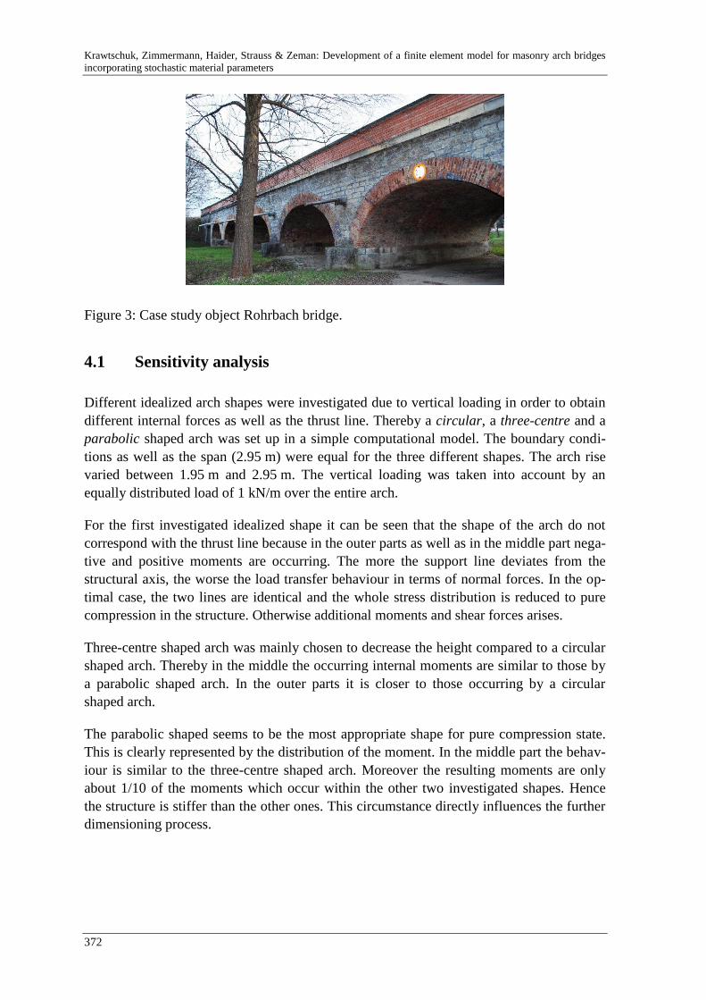
Krawtschuk, Zimmermann, Haider, Strauss & Zeman: Development of a finite element model for masonry arch bridges
incorporating stochastic material parameters
372
Figure 3: Case study object Rohrbach bridge.
4.1 Sensitivity analysis
Different idealized arch shapes were investigated due to vertical loading in order to obtain
different internal forces as well as the thrust line. Thereby a circular, a three-centre and a
parabolic shaped arch was set up in a simple computational model. The boundary condi-
tions as well as the span (2.95 m) were equal for the three different shapes. The arch rise
varied between 1.95 m and 2.95 m. The vertical loading was taken into account by an
equally distributed load of 1 kN/m over the entire arch.
For the first investigated idealized shape it can be seen that the shape of the arch do not
correspond with the thrust line because in the outer parts as well as in the middle part nega-
tive and positive moments are occurring. The more the support line deviates from the
structural axis, the worse the load transfer behaviour in terms of normal forces. In the op-
timal case, the two lines are identical and the whole stress distribution is reduced to pure
compression in the structure. Otherwise additional moments and shear forces arises.
Three-centre shaped arch was mainly chosen to decrease the height compared to a circular
shaped arch. Thereby in the middle the occurring internal moments are similar to those by
a parabolic shaped arch. In the outer parts it is closer to those occurring by a circular
shaped arch.
The parabolic shaped seems to be the most appropriate shape for pure compression state.
This is clearly represented by the distribution of the moment. In the middle part the behav-
iour is similar to the three-centre shaped arch. Moreover the resulting moments are only
about 1/10 of the moments which occur within the other two investigated shapes. Hence
the structure is stiffer than the other ones. This circumstance directly influences the further
dimensioning process.
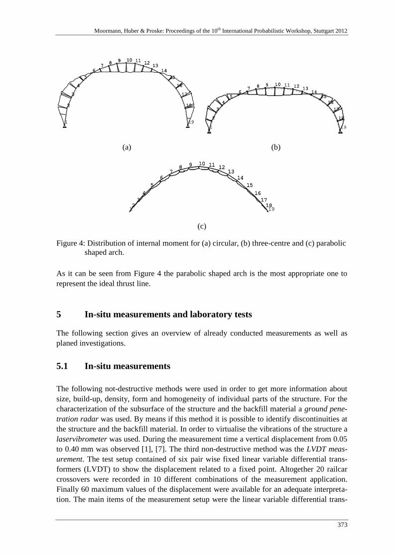
Moormann, Huber & Proske: Proceedings of the 10th International Probabilistic Workshop, Stuttgart 2012
373
(a)
(b)
(c)
Figure 4: Distribution of internal moment for (a) circular, (b) three-centre and (c) parabolic
shaped arch.
As it can be seen from Figure 4 the parabolic shaped arch is the most appropriate one to
represent the ideal thrust line.
5 In-situ measurements and laboratory tests
The following section gives an overview of already conducted measurements as well as
planed investigations.
5.1 In-situ measurements
The following not-destructive methods were used in order to get more information about
size, build-up, density, form and homogeneity of individual parts of the structure. For the
characterization of the subsurface of the structure and the backfill material a ground pene-
tration radar was used. By means if this method it is possible to identify discontinuities at
the structure and the backfill material. In order to virtualise the vibrations of the structure a
laservibrometer was used. During the measurement time a vertical displacement from 0.05
to 0.40 mm was observed [1], [7]. The third non-destructive method was the LVDT meas-
urement. The test setup contained of six pair wise fixed linear variable differential trans-
formers (LVDT) to show the displacement related to a fixed point. Altogether 20 railcar
crossovers were recorded in 10 different combinations of the measurement application.
Finally 60 maximum values of the displacement were available for an adequate interpreta-
tion. The main items of the measurement setup were the linear variable differential trans-
Krawtschuk, Zimmermann, Haider, Strauss & Zeman: Development of a finite element model for masonry arch bridges
incorporating stochastic material parameters
374
formers. They should record the displacements of the thread rods caused by the reaction of
the structure to the loading due to railcars.
From the obtained values of the measurement campaign it can be considered that the forces
from the crown along the diagonals go down to the abutments and the springer [5].
5.2 Laboratory tests
To obtain basic material parameters as well as their scatter laboratory tests on single bricks
were conducted. In a first test sequence compressive tests on normal sized bricks (25 x 12
x 6.5 cm) according to EN 772-1 [3] were carried out. The mean value of compressive
strength results in fb = 21.3 MPa, standard deviation s = 1.425 MPa and coefficient of vari-
ation cov = 0.0669. Based on this data the program FReET was used to fit a probability
density function (pdf) to the given data set. To choose the most appropriate pdf the Kol-
mogorov Smirnov test statistic was used [1]. This results in a Weibull distribution with m =
21.3, s = 1.425, b = 27.607 MPa. Additionally, tests should be performed with different
loading directions in order to obtain the compressive strength of bricks with respect to the
loading direction.
Beside the small scale testing one arch of the Rohrbach bridge will be reconstructed in the
scale 1:2. The arch will be built with bricks in compliance to the real structure and sup-
ported by artificial abutments. The backfill material can be varied with regards to its mix-
ture.
6 Conclusions
In this contribution it is shown how on the base of adequate measurement data and survey-
ing a FE-model of an existing masonry arch bridge can be set up for the evaluation process
of the bearing capacity as well as to incorporate stochastic properties. To determine the
most unfavourable shape of the arch a sensitivity analysis regarding the thrust line of three
possible arch shapes was carried out. For an increase of the accuracy and the practicability
of the model on the one hand laboratory tests were and are going to be performed to de-
termine the correlation of the measured values on the real object and the measured values
on a scale model; and on the other hand small scale tests on specimens taken from brick
stones under variable angles. These variable angles determine the variable loading direc-
tion which occurs on existing structures. Based on test results performed under a vertical
loading situation, which are already available, this extension to various angles will help to
characterize the material parameters in an appropriate way.
7 Acknowledgement
The support of the experimental investigations by the project CZ.1.07/2.3.00/30.0005 of
Brno University of Technology is gratefully acknowledged. Additionally the financial sup-

Moormann, Huber & Proske: Proceedings of the 10th International Probabilistic Workshop, Stuttgart 2012
375
port by the research projects ILATAS and NANUB are acknowledged. Further we would
like to thank Wienerberger for the provision of bricks for testing.
8 References
[1] Ang, A.H.-S.; Tang, W.H.: Probability Concepts in Engineering. John Wiley &
Sons, Inc. 2007
[2] Dengg, F.; Mendlig K.; Krawtschuk A.: Performing of non-destructive measurement
methods on existing arch bridge structures, Proceedings of the 3rd International
Symposium on Life-Cycle Civil Engineering, IALCCE 2012
[3] EN 772-1: Methods of test for masonry units – part 1: Determination of compressive
strength, 2000.
[4] Krawtschuk, A.; Strauss, A.; Wendner, R.; Zeman, O.: Inspection and Lifetime As-
sessment for Arch Bridges, in: Humberto Ramos R.; Guilherme Aris Parsekian
(Eds.), Proceedings of 15th International Brick And Block Masonry Conference;
ISBN: 978-85-63273-09-3, 2012
[5] Krawtschuk A.; Zeman, O.; Strauss, A.; Scheidl C.; Proske D.: Optimised monitor-
ing concepts for historical masonry arch bridges, Proceedings of the 3rd Internation-
al Symposium on Life-Cycle Civil Engineering, IALCCE 2012
[6] Proske, D.; van Gelder, P.: Safety of Historical Arch Bridges, Springer, Heidelberg,
2009
[7] Scheidl, C.; Chiari, M.; Kaitna, R.; Müllegger, M.; Krawtschuk, A.; Zimmermann,
T.; Proske, D.: Analysis debris-flow impact models, based on a small scale model-
ling approach, Surveys in Geophysics, online first, 2012
[8] Strauss, A.; Krawtschuk, A.; Wendner, R.; Frangopol, D.M.; Bergmeister, K.: Moni-
toring based assessment of a jointless bridge. Proceedings of 6th International Con-
ference on Bridge Maintenance, Safety and Management, IABMAS 2012, Italy,
2012
[9] UIC Code 778-3: Recommendations for the inspection, assessment and maintenance
of masonry arch bridges, April 2011
[10] Zimmermann, T.; Krawtschuk, A.; Strauss, A.; Wendner, R.: Extreme value statistics
for the life-cycle assessment of masonry arch bridges. Proceedings of 6th Interna-
tional Conference on Bridge Maintenance, Safety and Management, IABMAS 2012,
Italy, 2012

Krawtschuk, Zimmermann, Haider, Strauss & Zeman: Development of a finite element model for masonry arch bridges
incorporating stochastic material parameters
376

377
Mitteilungen des Instituts für Geotechnik
der Universität Stuttgart
Mitteilungen des Baugrundinstitutes Stuttgart
(Institut für Grundbau und Bodenmechanik)
der Universität Stuttgart
Hrsg.: Prof. Dr.-Ing. Dr. h.c. U. Smoltczyk
Nr. 01 Thamm, B. R. (1974) Anfangssetzungen und
Anfangsporenwasserüberdrücke
eines normalverdichteten wasser-
gesättigten Tones
Nr. 02 Gußmann, P. (1975) Einheitliche Berechnung von
Grundbruch und Böschungsbruch
Nr. 03 Feeser, V. (1975) Die Bedeutung des
Kalziumkarbonats für die
bodenphysikalischen
Eigenschaften vom Löß
Nr. 04 Du Thin, K. (1976) Standsicherheit von Böschungen:
Programm-Dokumentation
Nr. 05 Smoltczyk, U.
Pertschi, O.
Hilmer, K.
(1976) Messungen an Schleusen in der
UDSSR. Schleusennorm der
UDSSR (SN 30365)

Mitteilungen des Instituts für Geotechnik
378
Nr. 06 Hilmer, K. (1976) Erddruck auf
Schleusenkammerwände
Nr. 07 Laumans, Q. (1977) Verhalten einer ebenen, in Sand
eingespannten Wand bei nicht-
linearen Stoffeigenschaften des
Bodens
Nr. 08 Lächler, W. (1977) Beitrag zum Problem der Teil-
flächenpressung bei Beton am Bei-
spiel der Pfahlkopfanschlüsse
Nr. 09 Spotka, H. (1977) Einfluß der Bodenverdichtung
mittels Oberflächenrüttelgeräten
auf den Erd-druck einer
Stützwand bei Sand
Nr. 10 Schad, H. (1979) Nichtlineare Stoffgleichungen für
Böden und ihre Verwendung bei
der numerischen Analyse von
Grundbau-aufgaben
Nr. 11 Ulrich, G.
(1980) Verschiebungs- und
kraftgesteuerte Platten-
druckversuche auf
konsolidierenden Böden
Gußmann, P. Zum Modellgesetz der
Konsolidation
Nr. 12 Salden, D. (1980) Der Einfluß der Sohlenform auf
die Traglast von Fundamenten

Mitteilungen des Instituts für Geotechnik
379
Nr. 13 Seeger, H. (1980) Beitrag zur Ermittlung des
horizontalen Bettungsmoduls von
Böden durch Seitendruckversuche
im Bohrloch
Nr. 14 Schmidt, H.H. (1981) Beitrag zur Ermittlung des
Erddrucks auf Stützwände bei
nachgiebigem Baugrund
Nr. 15 Smoltczyk, U.
Schweikert, O.
(1981) Vorstudie über bauliche
Alternativen für
Durchgangsstraßen in Siedlungen
Nr. 16 Malcharek, K.
Smoltczyk, U.
(1981) Vergleich nationaler Richtlinien
für die Berechnung von
Fundamenten
Nr. 17 Gruhle, H.D. (1981) Das Verhalten des Baugrundes
unter Einwirkung vertikal
gezogener Ankerplatten als
räumliches Problem des
Erdwiderstandes
Nr. 18 Kobler, W. (1982) Untersuchungen über Böschungs-
und Grundbruch bei begrenzten
Lastflächen
Nr. 19 Lutz, W. (1983) Tragfähigkeit des geschlitzten
Baugrunds neben Linienlasten

Mitteilungen des Instituts für Geotechnik
380
Nr. 20 Smoltczyk, U. (1983) Studienunterlagen
“Bodenmechanik und
Grundbau“; überarbeitete
Ausgabe 1993
Nr. 21 Schweikert, O. (1984) Der Einfluß des
Böschungswinkels auf die
Berechnung des aktiven
Erddrucks
Nr. 22 Vogt, N. (1984) Erdwiderstandsermittlung bei
monotonen und wiederholten
Wand-bewegungen in Sand
Nr. 23 Buchmaier, R. (1985) Zur Berechnung von Kon-
solidationsproblemen bei nicht-
linearem Stoffverhalten
Nr. 24 Schad, H.
Smoltczyk, U.
(1985) Möglichkeiten der Böschungs-
sicherung bei kleinen Baugruben
Schad, H.
Zoller, P.
Sonderkonstruktionen der
Böschungssicherung
Nr. 25 Gußmann, P. (1986) Die Methode der Kinematischen
Elemente
Nr. 26 Steinmann, B. (1985) Zum Verhalten bindiger Böden
bei monotoner einaxialer
Beanspruchung
Nr. 27 Lee, S.D. (1987) Untersuchungen zur
Standsicherheit von Schlitzen im
Sand neben Einzelfundamenten

Mitteilungen des Instituts für Geotechnik
381
Mitteilungen des
Instituts für Geotechnik der Universität Stuttgart
Hrsg.: Prof. Dr.-Ing. Dr. h.c. U. Smoltczyk
Nr. 28 Kolb, H. (1988) Ermittlung der Sohlreibung von
Gründungskörpern unter
horizontalem kinematischen
Zwang
Nr. 29 Ochmann, H. (1988) Ebene Grenzzustände von
Erdböschungen im
stochastischen
Sicherheitskonzept
Nr. 30 Breinlinger, F. (1989) Bodenmechanische
Stoffgleichungen bei großen
Deformationen sowie Be- und
Entlastungsvorgängen
Nr. 31 Smoltczyk, U.
Breilinger, F.
Schad, H.
Wittlinger, M.
(1989) Beitrag zur Bemessung von
Tunneln in offener Bauweise
Nr. 32 Gußmann, P.
Schanz, T.
Smoltczyk, U.
Willand, E.
(1990) Beiträge zur Anwendung der
KEM (Erddruck, Grundbuch,
Standsicher-heit von
Böschungen)
Nr. 33 Gruhle, H.D. (1990) Der räumliche Erdwiderstand
vor überwiegend horizontal
belasteten Ankerplatten

Mitteilungen des Instituts für Geotechnik
382
Nr. 34 Henne, J. (1995) Zur Bewehrung von verformten
Bodenschichten durch Einsatz
zugfester Geokunststoffe
Nr. 35 Wittlinger, M. (1994) Ebene
Verformungsuntersuchungen zur
We-ckung des Erdwiderstandes
bindiger Böden
Nr. 36 Schad, H.
(1992) Zeit- und geschwindigkeits-
abhängiges Materialverhalten in
der Geotechnik – Experimentelle
Erfassung und numerische
Analyse
Nr. 37 Belz, I. (1992) Zur Ermittlung dynamischer
Boden-kennwerte in situ aus der
Systemantwort des Erregers
Nr. 38 Ma, J. (1994) Untersuchungen zur
Standsicherheit der durch
Stützscheiben stabilisierten
Böschungen
Nr. 39 Smoltczyk, U. (1994) Sonderheft: 25 Jahre Lehre und
Forschung in der Geotechnik
Nr. 40 Rilling, B. (1994) Untersuchungen zur
Grenztragfähigkeit bindiger
Schüttstoffe am Beispiel von
Lößlehm

Mitteilungen des Instituts für Geotechnik
383
Mitteilungen des
Instituts für Geotechnik der Universität Stuttgart
Hrsg.: Prof. Dr.-Ing. P.A. Vermeer
Nr. 41 Vermeer, P.A. (1996) Deponiebau und Geotechnik
Nr. 42 Vermeer, P.A. (1997) Baugruben in Locker- und Fest-
gestein
Nr. 43 Brinkmann, C. (1998) Untersuchungen zum Verhalten
von Dichtungsübergängen im
Staudammbau
Nr. 44 Fiechter-Scharr,
I.
(1998) Beeinflussung von Erdbaustoffen
durch Beimischen eines organo-
philen Bentonits
Nr. 45 Schanz, T. (1998) Zur Modellierung des
mechanischen Verhaltens von
Reibungsmaterialien
Nr. 46 Akinrogunde,
A.E.
(1999) Propagation of Cement Grout in
Rock Discontinuities Under
Injection Conditions
Nr. 47 Vogt-Breyer, C. (1999) Experimentelle und numerische
Untersuchungen zum
Tragverhalten und zur
Bemessung horizontaler
Schraubanker
Nr. 48 Vermeer, P.A. (1999) Neue Entwicklungen in der
Geotechnik

Mitteilungen des Instituts für Geotechnik
384
Nr. 49 Marcher, T. (2002) Resultate eines
Versuchsprogramms an Beaucaire
Mergel
Nr. 50 Marcher, T. (2003) Nichtlokale Modellierung der
Entfestigung dichter Sande und
steifer Tone
Nr. 51 Ruse, N.M. (2004) Räumliche Betrachtung der
Stand-sicherheit der Ortsbrust
beim Tunnelvortrieb
Nr. 52 Beutinger, P.H. (2005) Ein geotechnischer Beitrag zur
Standsicherheit mobiler Bau-
maschinen
Nr. 53 Wehnert, M. (2006) Ein Beitrag zur drainierten und
undrainierten Analyse in der
Geotechnik
Nr. 54 Möller, S. C. (2006) Tunnel induced settlements and
forces in linings
Nr. 55 Benz, T. (2007) Small-Strain Stiffness of Soils and
its Numerical Consequences
Nr. 56 Abed, A. (2008) Numerical Modeling of
Expansive Soil Behavior

Mitteilungen des Instituts für Geotechnik
385
Nr. 57 Hintner, J. (2008) Analyse der Fundamentver-
schiebungen infolge vertikaler
und geneigter Belastung
Nr. 58 Russelli, C. (2008) Probabilistic Methods applied to
the Bearing Capacity Problem
Nr. 59 Peña Olarte,
A.A.
(2008) Influence of Particle Shape on the
Global Mechanical Response of
Granular Packings:
Micromechanical Investigation of
the Critical State in Soil
Mechanics
Nr. 60 Neher, H. P. (2008) Zeitabhängiges Materialverhalten
und Anisotropie von weichen
Böden – Theorie und Anwendung
Nr. 61 Vermeer, P.A. (2008) Von der Forschung zur Praxis:
Symposium zum 80. Geburtstag
von Prof. U. Smoltczyk
Nr. 62 Satibi, S. (2009) Numerical Analysis and Design
Criteria of Embankments on
Floating Piles
Nr. 63 Lächler, A. (2009) Bedeutung herstellungsbedingter
Einflüsse auf das Trag- und
Verformungsverhalten von
Schlitzwänden

Mitteilungen des Instituts für Geotechnik
386
Nr. 64 Möllmann, A. (2009) Probabilistische Untersuchung
von Hochwasserschutzdeichen
mit analytischen Verfahren und
der Finite-Elemente-Methode

Mitteilungen des Instituts für Geotechnik
387
Mitteilungen des
Instituts für Geotechnik der Universität Stuttgart
Hrsg.: Prof. Dr.-Ing.habil. Ch. Moormann
Nr. 65 Moormann, Ch. (2011) 7. Stuttgarter Geotechnik-
Symposium
Nr. 66 Beuth, L. (2012) Formulation an Application of a
Quasi-Static Material Point
Method
Nr. 67 Moormann, Ch.,
Huber, M.,
Proske, D.
(2012) Proceedings of the
10th International Probabilistic
Workshop

Mitteilungen des Instituts für Geotechnik
388