14.581 international trade lecture 20: trade and growth...

14.581 International Trade— Lecture 20: Trade and Growth Empirics —

14.581

Week 11

Fall 2011

14.581 (Week 11) Trade and Growth Empirics Fall 2011 1 / 56

Plan for Today’s Lecture

Brief introduction.

Neoclassical growth models in open economies:

How large are the terms-of-trade effects that come with growth?

Does trade liberalization promote income convergence (as FPEtheorem would suggest)?

Structural Transformation in open economies.

Endogenous growth models in open economies:

What evidence is there for international knowledge spillovers?

Does technology embodied in physical goods (intermediate inputs orcapital equipment) lead to important international technology transfer?

Brief discussion of other effects: market size, competition.

Brief discussion of other ‘trade and growth’ channels.


Introduction: Trade and Growth Empirics

“Trade and Growth” is a field that is of great importance:

Obviously growth is important so understanding whether there isanything that countries can do to promote it (eg trade policy) is clearlyimportant.

Also, studies like Feyrer (2009) suggest that the empirical gains fromtrade/openness are quite a bit larger than those predicted in any staticmodel of trade. Perhaps ‘dynamic effects’ of openness (ie whereopenness changes technology) can have a bearing on this puzzle.

This is also a field that should be ripe for empirical work:

Theory is fundamentally ambiguous about how openness affects growthrates.

Additionally, theories often postulate concepts like ‘technologicalspillovers’ with some parameter governing the extent to which thesespillovers can occur. It is up to empirical work to measure those(extremely important) parameters.



Brief introduction.

Neoclassical growth models in open economies:How large are the terms-of-trade effects that come with growth?



Endogenous growth models in open economies:What evidence is there for international knowledge spillovers?





Neoclassical Growth Models in Open Economies

We’ll cover 3 papers:

Acemoglu and Ventura (QJE 2002) empirics

Ben-David (QJE 1993) on convergence

Structural Transformation in open economies


Acemoglu and Ventura (2002)

In the previous lecture we discussed the theory part of this paper.

Recall the key insights:

AK model: in autarky countries would grow at different rates.

Add simple (Armington with no trade costs) trade model: countriesgrow at the same rate.

Why? As a country accumulates K and produces more of its good, itfloods the world market with this good. This depresses the price of itsexport good, and hence its terms of trade. Lower terms of trade harmsthe country’s GDP (ie the return on its K). Lower return means lessincentive to accumulate.

Here we briefly cover the empirical side of AV (2002).

The punchline is that the forces for convergence created by TOT arelarge—too large in fact.


AV (2002): Question 1: Are growth rates similar aroundthe world?Yes. 660 QUARTERLY JOURNAL OF ECONOMICS

2

I~~~~~~~~~~~~~~~~T >~~~~~~~~~~~~~~ 1 KG SPflN' IRISR S

0 O~~~~~~~~~O OAN off w VEN

2~~~~~~~~~~m _ JIC G

o 0 SHA y IRN 0)T 0)

E -1 - G NIC 0

O ~~~~~CP 6CIWG GUY

-- SEN ZWE

BfN B9PA MLI TCD

I ~ ~~I I I -2 -1 0 1 2

Log Income in 1960 rel. to avg.

FIGURE I Log of Income per Worker in 1990 and 1960 Relative to World Average from

the Summers and Heston [1991] Data Set The thick line is the 45 degree line.

Existing frameworks for analyzing these questions are built on two assumptions: (1) "shared technology" or technological spillovers: all countries share advances in world technology, albeit, in certain cases, with some delay; (2) diminishing returns in production: the rate of return to capital or other accumulable factors declines as they become more abundant. The most popular model incorporating these two assumptions is the neoclassical (Solow-Ramsey) growth model. All countries have access to a common technology, which improves exogenously. Diminishing returns to capital in production pull all countries toward the growth rate of the world technology. Differences in economic policies, saving rates, and technology do not lead to differences in long-run growth rates, but in levels of capital per worker and income. The strength of diminishing returns determines how a given set of differences in these

Pritchett [1997] for the widening of the world income distribution since 1870 and Acemoglu, Johnson, and Robinson [2001b] for the reversal in relative economic rankings over the past 500 years, and widening over the past 200 years.


AV (2002): Question 2: Do Terms of Trade Move Enough?

Recall that country i ’s income level (yi ) is given by:

yi = µip1−σi Y (1)

µi = index of country i ’s technology level.Y = world GDP level (Y =

∑i yi ).

σ = elasticity of substitution across world (Armington) varieties (withσ > 1).

Taking logs this implies that TOT evolve over time (growth of TOT= πit) as:

πit =git − xtσ − 1

+ ∆ lnµit (2)

git = growth rate of country i ’s income.xt = growth rate of world income.Recall that price of Y is taken as the numeraire.



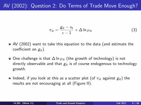
πit =git − xtε− 1

+ ∆ lnµit (3)

AV (2002) want to take this equation to the data (and estimate thecoefficient on git).

One challenge is that ∆ lnµit (the growth of technology) is notdirectly observable and that git is of course endogenous to technologygrowth.

Indeed, if you look at this as a scatter plot (of πit against git) theresults are not encouraging at all (Figure II).



676 Q

UA

RT

ER

LY

JOU

RN

AL

O

F E

CO

NO

MIC

S

0 0

0 0

z 8

50 L

fi C

3

E

0

0 m

;1

Q.

~ ~ ~ o~~~~~~~0c

O

___________ _

O

O_

O

>H

"OM

OJ

epel jo sw

iJ@

rO %

0

0 01

0~~~~~~~~~~~0

40 *

C00

0 0

co X

zNo

0 0I 0

) I

'O

0 0

C.~~~2 0>

a) >

o C

z -o~~~~~0 0

g ~

~ ~

~~~~~ Q

. -o.

L'70

0- C

D

coJ9 cO

2~~~~~~~~~~~ 0)

Ill Ill

I1 l

0 *

0 E

: 8pi 0SW

li

8p0~~ JO



πit =git − xtε− 1

+ ∆ lnµit (4)

But the model suggests an IV: conditional convergence (if the countryis out of steady-state):

git = −β ln yi ,t−1 + θZit + uit (5)

Here β is the (conditional) convergence coefficient.And Zit is a vector of variables that characterize where a country’ssteady-state level is.

AV (2002) use ln yt−1 as the excluded IV, and of course thereforeremember to include Zt in both the first and second stages.


AV (2002): Question 2: Do Terms of Trade Move Enough?Once AV instrument for gt the results are more encouraging

682 Q

UA

RT

ER

LY

JOU

RN

AL

O

F E

CO

NO

MIC

S

LO

L

00 '-4

0 0

U) ~~~~~~~~~~~~~~~l

01~~~ O

0

0

O

0~ I

-

U)

0

C

o /)

Um

co 00

e a!

U)

0). 0

z _ _

_ _

_ _

_ _

_ _

_ _

_

x w

~

~ ~

.

oOO

J N

p) JoSJUL

Ifl!UQ

w~~~~~~~

0 J:

~ ~

~ ~

bj- [itt

CC

) N

O,

o. o,

o .

O.

O

,

C?~~~~~~~

EH

M

0Wj

ap0J 4-4Jl

eps8

E

O

fi /

O2

I= 0

zZ

0 00

4

C,

Xi

U)} 0,

- t,

U))

0 0)a

/ Z

. to

U)

403 N

C t,

o ,

o o

UU

U

o .

? ?

-

_WoJfl3 epe l }0

SWJ8l

ienP!uC

O

U)

Z

U)

l

E

co C

zcJoJ U

)UJ[J

SJJ T

P'U

J


AV (2002): Question 2: Do Terms of Trade Move Enough?THE WORLD INCOME DISTRIBUTION 679

TABLE I IV REGRESSIONS OF GROWTH RATE OF TERMS OF TRADE

Adding Adding Adding Main Detailing political change change Nonoil

regression schooling indicat in Sch in Sch sample

(1) (2) (3) (4) (5) (6)

Panel A: Two-stage least squares

GDP Growth -0.595 -0.578 -0.458 -0.561 -0.455 -0.620 1965-1985 (0.265) (0.261) (0.221) (0.248) (0.187) (0.354)

Years of -0.001 -0.002 -0.000 -0.001 schooling 1965 (0.002) (0.002) (0.002) (0.002)

Years of -0.002 primary (0.003) schooling 1965

Years of -0.002 secondary (0.006) schooling 1965

Years of higher 0.019 schooling 1965 (0.034)

Log of life 0.043 0.045 0.034 0.020 0.046 expectancy (0.024) (0.024) (0.021) (0.027) (0.030) 1965

OPEC dummy 0.091 0.090 0.092 0.086 0.087 (0.009) (0.009) (0.009) (0.010) (0.009)

War dummy -0.013 (0.005)

Political 0.007 instability (0.023)

Log black -0.005 market (0.012) premium

Change in years 0.008 0.009 of schooling (0.004) (0.003) 1965-1985

Change in log of -0.000 -0.042 life expectancy (0.078) (0.045) 1965-1985

Panel B: First-stage for GDP growth

Log of GDP 1965 -0.019 -0.020 -0.024 -0.020 -0.020 -0.016 (0.004) (0.004) (0.004) (0.004) (0.004) (0.004)

R2 0.35 0.36 0.54 0.47 0.47 0.34

Panel C: Ordinary least squares

GDP Growth 0.037 0.037 0.038 0.041 -0.005 0.116 1965-1985 (0.106) (0.107) (0.107) (0.112) (0.103) (0.114)

N. of obs 79 79 70 79 79 74

"Growth Rate of Terms of Trade" is measured as the annual growth rate of export prices minus the growth rate of import prices. The OPEC dummy takes value 1 for five countries in our sample (Algeria, Indonesia, Iran, Iraq, and Venezuela). The political instability variable is the average of the number of assassinations per million inhabitants per year and the number of revolutions per year, the war variable is a dummy for countries that fought at least one war over the period 1965-1985, and the log black market premium is the average of the logarithm of the black market premium over the period 1965-1985. All the data are from the Barro-Lee data set.

Excluded instrument is log of output in 1965 in columns (1), (2), (3), and (4) and (6), while in column (5) excluded instruments are log of output in 1965, years of schooling in 1965, and the log of life expectancy in 1965.


AV (2002): Question 3: Are the Results Sensible?

Effect of growth on TOT:Coefficient (from 2SLS) in column 1 is -0.6. Structural interpretationof regression says that this is 1

σ−1 , or σ=2.6.This is reasonable compared to outside estimates of the Armingtonelasticity.

Convergence coefficient near steady-state:

This is β = τ(ρ+x∗)σ , where τ is the share of tradables in GDP (eg,

generously, around 0.3) and x∗ is the steady-state world growth rate.All of this implies β = 0.011, which is smaller than the β = 0.02 thatBarro (1991) finds.But we are not allowing for any other source of diminishing returns, orfor any technological catch-up.

The steady-state level of each country’s GDP:

This is y∗ = µφ(σ−1)/τ(

sx∗

)(σ−1)/τ.

Mankiw, Romer and Weil (QJE 1992) estimate something similar andfind a coefficient on s of around 2.With σ = 2.6 and τ = 0.3, the coefficient on s is too low.



Brief introduction.










Ben-David (QJE, 1993)

Ben-David (1993) asks whether we see faster convergence amongcountries that trade more.

He focuses on countries within free trade areas (FTAs) to proxy for‘countries that trade more’.

Paper starts with the European Economic Community (EEC).

And then moves on to wider FTAs (EFTA and Canada-USA).


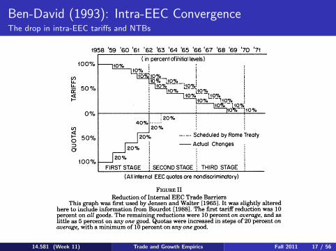
Ben-David (1993): Intra-EEC ConvergenceThe drop in intra-EEC tariffs and NTBs

EQUALIZING EXCHANGE 657

1958 '59 '60 '61 '62 '63 '64 '65 '66 '67 '68 '69 '70 '71

`100% 0 ( in percent of initial levels)

1100 10%

CO j 0%-10% i i LL 50%i ?;i0% @jO LL 10 110 % 10 ~ 500/a 10% jjO%

. . | .. ll~ 1 0% 0%

. l . ltio'O%

.20% 40% :......,

co ~~~~20%'i

;!50% AScheduled by Rome Treaty 3 = Actual Changes

100%~~~~~~~~~~~0/ 1100/

FIRST STAGE ,SECONDSSTAGE bTHIRD STAGE

(All internal EEC quotas are nondiscriminatory)

FIGURE II Reduction of Internal EEC Trade Barriers

This graph was first used by Jensen and Walter [1965]. It was slightly altered here to include information from Bourdot [1988]. The first tariff reduction was 10 percent on all goods. The remaining reductions were 10 percent on average, and as little as 5 percent on any one good. Quotas were increased in steps of 20 percent on average, with a minimum of 10 percent on any one good.

replaced by the Common Customs Tariff. The main difference between the EEC tariff reductions and those imposed by GATT was in their scope. While GATT negotiations produced tariff cuts on a commodity-by-commodity basis, the EEC lowered them on all goods at once, in a step-by-step progression specified in advance at the time of the signing of the Treaties of Rome. This across-the- board form of tariff reductions did in fact have some exceptions, particularly regarding some agricultural products that were ex- empted from the overall timetable and were instead governed by special regulations. Internal agricultural quotas, as well as minimum prices, came to be replaced by variable levies.

It should also be noted that only the initial tariff reduction of 10 percent in 1959, and the final removal of all customs duties in 1968, were to be applied uniformly across all goods. Countries were given discretion in the degree of reduction they imposed on each commodity, as long as they averaged the 10 percent drops agreed upon in the original timetable. They were further required to reduce the internal duties on each product by at least 25 percent and 50 percent, at the end of the first and second stages of the transition period, respectively.


Ben-David (1993): Intra-EEC ConvergenceTariff changes did affect trade flowsEQUALIZING EXCHANGE 659

a.

C 12

.0 E10 F

8 8

co 0)

E '~ 0 O. II (D 1950 1960 1970 1980 -3 Year > 0 Intra-EEC Imports 0 Non-EEC Industrial Countries

A Imports from Non-oil LDC's A Imports from Oil Producing LDC's

FIGURE IV

Origin of Imports, as a Percent of GDP

III with the ratio of total intra-EEC imports to GDP.8 In the pretransition period, the volume of imports from the rest of the world was stable, at approximately 11 percent of GDP. During these years there was a slight, though significant, rise in the intra-EEC imports to GDP ratio. This coincided with the partial liberalization that had already begun between the countries which would later form the European Economic Community.

During the transition period that followed, imports from the rest of the world declined a little, relative to GDP, while the ratio of intra-EEC trade doubled. In the twelve years following 1973, when nearly all the barriers on trade between the members of the European Economic Community had been removed, the fraction of intra-EEC trade, out of GDP, stabilized and remained between 10 and 11 percent. This compares with a rise in the ratio of non-EEC imports to GDP, which was due in large part to the liberalization of trade with other industrialized countries (which included the Community's new members). This is illustrated in Figure IV. The less pronounced, but significant, increase in imports from the

8. Data source: IMF, International Financial Statistics and Direction of Trade Statistics.


Ben-David (1993): Intra-EEC ConvergenceDramatic reduction in intra-EEC income disparities. But was this phenomenon alreadyunderway prior to WWII?

662 QUARTERLY JOURNAL OF ECONOMICS

E 8 0.4

-

0

6. 0.3 _

C

0.2

(B 0.1

1 870 1890 1910 1930 1950 1970

Year

FIGURE VII Per Capita Income Dispersion: Between Belgium, France, the Netherlands, and

Italy, 1870-1979

(v's) for the founding members of the EEC all the way back to 1870.10 The standard deviations displayed in Figure VII measure the income dispersion without Germany. The country is omitted to show that the postwar convergence which took place was not simply an outcome of German rebuilding following the war."1

The behavior of the or's clearly indicates that, during the prewar years, neither of the above two scenarios appears to hold. The dispersion of real per capita incomes was fairly stable from 1870 until the mid-1950s, with the or's fluctuating between 0.194 and 0.268. Only after the onset of trade liberalization did the standard deviations exhibit a level change (the minimum level of 0.104 was attained in 1968, the final year of the transition period).

Income Behavior of the Three New EEC Member-Countries

Shifting the focus to the next three countries to join the EEC (Ireland, Denmark, and the United Kingdom) examines the ques-

10. Maddison's data include all of the original EEC countries, with the exception of the smallest, Luxembourg. From Summers and Heston's data, however, it can be shown that exclusion of Luxembourg does not appreciably alter the main conclusions enumerated above. Therefore, its omission here should not be considered too serious a problem.

11. Germany was always among the poorest, in per capita terms, of the six countries. Today, it is one of the wealthiest countries in Europe. As a result of its heightened prosperity, it might be claimed that all of the convergence that has been witnessed within the EEC is due to the behavior of Germany. Thus, its exclusion should bias the results away from convergence.


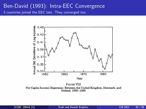
Ben-David (1993): Intra-EEC Convergence3 countries joined the EEC late. They converged too.


tion of whether their income differentials behaved in a manner similar to those of the original Six during the entire postwar period, despite the differences in the timing of their trade reforms. Furthermore, if these countries exhibited convergence upon elimination of their trade barriers, was this behavior any different than their preliberalization behavior?

Figure VIII displays the annual disparity among the Three. In contrast with the convergence that occurred among the Six, the or's of the Three actually increased until the mid-sixties. At that time the countries began to relax the trade restrictions that existed among themselves and later in the decade they began to liberalize trade with the Six. This coincided with a stabilization in the it's, followed by a reduction in the degree of income disparity. The rise in the income differentials of the Three during the eighties coincides with an increase in the ct's of the Six. This could be due to expansion of the EEC to include Greece (and later Spain and Portugal), as well as heightened benefits to LDCs.

Comparison of the EEC to Opposing Benchmarks

While the EEC countries have exhibited a significant reduction in the degree of income disparity among themselves, this has not been a prevalent feature of the international data. The remainder of this section focuses on a comparison of the EEC with opposing benchmark cases.

Wu 0.45 E 0

0' C 0.43 -

0

M0.41

C 0.39

W 0.37-

0.3

0.351

< 1950 1960 1970 1980

Year

FIGURE VIII Per Capita Income Dispersion: Between the United Kingdom, Denmark, and

Ireland, 1950-1985


Ben-David (1993): Intra-EEC ConvergenceRest of world was diverging (unconditionally) at this timeEQUALIZING EXCHANGE 665

1.2

E 0

1.0

o World (excl. EEC 6) 9 0.8 -

06 .? 0.6 -

U.S.States Top 25 (excl. EEC 6) 04

-~~~~~~ ~~E.E.C.

'a 0.2 C: C < 0 i

1934 1944 1954 1964 1974 1984

Year

FIGURE IX Comparison of Income Dispersions, 1929-1985

n

1.4 0

0.6 0

o 0.4 qa)

0.2

g 1950 1960 1970 1980

w Year

o EEC/US States A EEC/Mid 14(exclVen) o EEC/Top 25 * EEC/World 107

FIGURE X Ratio of Disparity in EEC to Disparity in Other Groups

(relative standard deviations)


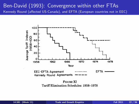
Ben-David (1993): Convergence within other FTAsKennedy Round (affected US-Canada), and EFTA (European countries not in EEC)


IV. LIBERALIZATION AND INCOME DISPARITY ELSEWHERE

While convergence has not appeared to be the dominant trend for most countries, there is evidence that income differentials among OECD countries have been declining during the postwar period. Although the EEC comprises a sizable proportion of these countries, not all the OECD convergence is due to EEC convergence. Furthermore, the timing of the EEC convergence was not identical to the timing among the other countries.

The impact of trade on convergence within the OECD becomes somewhat more plausible when one considers the origins of the OECD. Its predecessor, the OEEC (Organization for European Economic Cooperation), was established in 1948 to promote free trade within Europe and to provide suggestions regarding the distribution of American aid, which was contingent on relaxation of obstacles to trade. Most of the OEEC's success, as far as trade liberalization was concerned, came with the removal of up to 80 percent of the quantitative restrictions [Bourdot, 1988; Graduate Institute of International Studies, 1968] between its member countries, though it met with less success in eliminating tariff barriers.

In the 1960s the OEEC was supplanted by the OECD (Organi- zation for Economic Cooperation and Development) with the addition of non-European countries. Some of the trade liberalization within the OECD resulted from multilateral agreements under the auspices of the GATT, while a considerable amount of

100

x 80 _

9 60 -

00 U) 40

-

20 -.

A , . I . 1958 1962 1966 1970 1974 1978

Year

EEC-EFTA Agreement EFTA Kennedy Round Agreements

FIGURE XI Tariff Elimination Schedules: 1958-1978


Ben-David (1993): Convergence within other FTAsConvergence between US and Canada


0.24

o 0.20 -

(0

0.16 D 0 12 (0

J 0.08

,,0.04

0)

~~~~~ 0 ~ ~ ~ ~ V

1950 1960 1970 1980

Year

FIGURE XIII Gap in Per Capita Incomes: Between the United States and Canada, 1950-1985

Three times during this period, the United Kingdom Denmark, and Norway applied for EEC membership, finally signing the Treaty of Accession in January 1972. While Norway eventually opted to stay out of the EEC, the United Kingdom and Denmark, together with Ireland decided to join, becoming members of the EEC in January 1973. The remaining EFTA countries each tried to come to terms with the EEC during the sixties, but without success.

Austria, which ranked second in terms of per capita income among the five remaining countries before World War I, had fallen to last place by the end of World War II. After the Second World War, it rebounded dramatically, and this led to a steady decline in income differentials among the five throughout the postwar period. Austria, however, appears to be an outlier, as income differentials among the remaining countries (Switzerland, Sweden, Finland, and Norway) stayed fairly steady until the early sixties, beginning a slight decline during EFTA's liberalization period from 1961 through 1967. But the biggest decline in cr came after EFTA had abolished its internal trade barriers (Figure XIV).17 One possible explanation may be that, with the exception of the United King- dom, the size of the EFTA countries is very small (compared with the EEC) and the ratio of their internal trade to their external

17. Income disparity among all six EFTA countries (that is, with the inclusion of the United Kingdom and Denmark) was very similar to that of the four.


Ben-David (1993): Convergence within other FTAsConvergence within EFTA 6


0.20 E 0 c 0.18 -

o0160

C" 0

0.14

0

) 0.12

C C < oic?l I

1950 1960 1970 1980

Year

FIGURE XIV Per Capita Income Dispersion Among EFTA 6: Switzerland, Sweden, Denmark,

Norway, Finland, and the United Kingdom

trade is fairly small.18 A much larger proportion of EFTA's trade was with the EEC, so trade liberalization with the EEC may have had more of an impact on disparity within EFTA than its own, internal, liberalization.

Tariffs between EFTA and the EEC were reduced starting in mid-1968, in accordance with the Kennedy Round Agreements. Further agreements between the EEC and the EFTA countries provided for the continuation of this process, until the eventual elimination of nearly all tariffs on industrial goods by 1977 (the impact of this agreement on EFTA imports from the EEC may be seen in Figure XV).V9 In fact, not only did disparity within EFTA decline from 1968 through the mid-seventies, so also did the income gap between the EFTA and EEC mean incomes.

Table III gives an indication of how the timing of the convergence differed between the EEC and the other groups. The postwar period is divided into four periods. In the first period, which ran from 1951 to 1958 (the years prior to the formation of the EEC and

18. The ratio of EFTA 6's internal trade (measured by its imports) to its total imports rose from 17 percent (8 percent for the EFTA 4) prior to liberalization, to 22 percent (12 percent for the EFTA 4) by the end of the transition period in 1967. By comparison, total intra-EEC imports comprised 46 percent of total EEC imports by the end of their transition period, up from 30 percent at its inception.

19. Trade reform with the EFTA countries that became EEC members in the early seventies proceeded at the same pace as the overall liberalization between the EEC and the countries that remained in EFTA.


Ben-David (1993)

These are striking findings. But we need to remember some caveats:1 Other aspects of economic policy were liberalized as well in this time

period.

2 Mankiw, Romer and Weil (1992) find evidence for conditionalconvergence throughout the world, but not for unconditionalconvergence. Unfortunately, Ben-David (1993) is showing us plots (andrunning regressions) related to unconditional convergence. There is aserious risk that FTA countries have similar Solovian fundamentals andall we are seeing is conditional convergence. (But the timing of theconvergence is impressive, and a pure Solow story would require FTAmembers’ fundamentals to become more similar as they sign up to theFTA.)



Brief introduction.










Openness and the Structural Transformation

The ‘structural transformation’ (shifts in sectoral output shares asGDP grows) have received lots of recent attention.

Ngai and Pissarides (AER, 2007)Acemoglu and Guerrieri (JPE, 2008)Buera and Kaboski (2006, 2007).And others—“Baumol’s curse” being the foundation.

Most of this work (along with most of the work in the ‘growth’literature) works with an autarkic country model and then takes it tothe data.

This is probably misleading for thinking about growth (as, eg,Acemoglu and Ventura (2002) demonstrated).But it might be even worse for thinking about inter-sectoral issues,because trade means that countries’ inter-sectoral allocations areinterdependent. Matsuyama (JEEA, 2009) makes this point very nicely.Yi and Zhang (2010) and Teignier-Baque (2009, JMP) attempt toremedy this.



Brief introduction.










Openness and Endogenous Growth

Recall from previous (theory) lecture that the effect of openness ongrowth in endogenous growth models depends on:

1 The scope for technological spillovers. This should really be sub-dividedfurther into:

‘Knowledge spillovers’: transfer of technology that is not embodied inphysical inputs. Eaton and Kortum (IER, 1999) formalize this, but the‘model’ of knowledge spillover is just an exogenous diffusion process.‘Input trade’: transfer of technology that is embodied in physical inputs(intermediate inputs or ‘capital’). This is the mechanism in openeconomy versions of Romer-style engogenous growth (eg Grossman andHelpman book).

2 The ‘market size effect’. Openness creates larger markets, whichenlarges the gains from innovation and therefore makes firms want toinnovate more.

3 The ‘competition effect’. Larger markets have the down-side that a firmfaces higher competition and therefore gains less from any innovation.

We discuss empirical work motivated by these 3 phenomena.


Technological Spillovers and Openness

An enormous literature (surveyed by Keller (JEL, 2004)) hasattempted to measure technological spillover across countries (andpossibly even larger literature looks at spillovers within countries).

I will draw a distinction between:

‘Knowledge spillovers’: these leave no direct empirical trace, so they’reharder to pin down.

‘Input (intermediates and K) trade’: here we can actually track theflow of goods, and use prices, quantities and theories of input demandto quantify the effects of trade in ‘inputs’.



Brief introduction.










Knowledge Spillovers and Openness

A number of papers have looked at ‘knowledge spillovers’ across andwithin countries.

What do we mean by ‘knowledge spillovers’? A famous quote fromMarshall (1890):

“When an industry has thus chosen a locality...it is likely to staythere...so great are the advantages...The mysteries of the trade becomeno mysteries; but are as it were in the air...inventions and improvementsin machinery, in processes and the general organization of the businesshave the merits promptly discussed; if one man starts a new idea, it istaken up by others and combined with suggestions of their own...”


Knowledge Spillovers and Openness

A central challenge is to measure ‘knowledge’. Three approachesprevail:

1 Proxy for knowledge via inputs to knowledge: R&D expenditure.

2 Proxy for knowledge via outputs of knowledge: patents.

3 Proxy for knowledge via the effects of knowledge: TFP.

An ensuing challenge is how to regress one country’s ‘knowledge’ onanother country’s ‘knowledge’ and interpret the coefficient in a causalmanner.

The ‘peer effects’ literature in labor economics (eg Manski (ReStud,1993)) should make us very humble about the ability to do this.


Jaffe, Trajtenberg and Henderson (QJE 1993)

This was the first paper to use US patent data citations tosystematicaly document the geographic concentration of citations.

This is an extremely influential and highly-cited article (over 3000 onGoogle Scholar!)

The logic here:

An inventor (usually) “builds on the shoulders of giants” when comingup with a new product.

He/she is legally obliged (when filing a patent) to cite prior inventionsthat the present invention builds on.

The patent inspector also adds citations to the final published citation.


Jaffe, Trajtenberg and Henderson (QJE 1993): Results

Their finding is that citations (excluding self-cites) are more likely tooccur within the same US city, US state, and country then a ‘controlgroup’ would predict.

The ‘control group’ basically just adjusts for clustering of industries bygeography.

Eg, does Silicon Valley cite Silicon Valley because of knowledgespillovers or because everyone there is in the same industry?

We can easily control for industries because ‘industry’ is observed.But what about unobserved spatially correlated variables that affecteveryone in Silicon Valley?

This is one of the challenges of doing work on peer effects highlightedby Manski (1993).


Jaffe, Trajtenberg and Henderson (1993): Results590 QUARTERLY JOURNAL OF ECONOMICS

TABLE III GEOGRAPHIC MATCHING FRACTIONS

1975 Originating cohort 1980 Originating cohort

Top Other Top Other University corporate corporate University corporate corporate

Number of citations 1759 1235 1050 2046 1614 1210

Matching by country

Overall citation matching percentage 68.3 68.7 71.7 71.4 74.6 73.0

Citations excluding self-cites 66.5 62.9 69.5 69.3 68.9 70.4

Controls 62.8 63.1 66.3 58.5 60.0 59.6 t-statistic 2.28 -0.1 1.61 7.24 5.31 5.59

Matching by state



Controls 2.9 6.8 6.4 4.1 7.0 5.2 t-statistic 4.55 0.09 3.50 7.90 6.28 5.51

Matching by SMSA



Controls 1.0 1.3 1.2 1.1 3.6 2.3 t-statistic 6.43 4.80 8.24 9.57 6.28 5.52

Number of citations is less than in Table I because of missing geographic data for some patents. The t-statistic tests equality of the citation proportion excluding self-cites and the control proportion. See text for details.

At the SMSA level, 9 to 17 percent of total citations are localized. This again drops significantly when self-citations are excluded, but 4.3 percent of university citations, 4.5 percent of top corporate citations, and 8.7 percent of other corporate citations are localized excluding self-cites. This compares with control matching proportions of about 1 percent, and these differences are highly significant.


Coe and Helpman (EER, 1995)

Coe and Helpman (1995) look at international spillovers of R&Dexpenditure, and attempt to further restrict attention to spilloversoccurring through trading relationships.

Again, this is an enormously influential paper (with almost 3200Google Scholar cites, Helpman’s highest article!)

They estimate the following regression:

lnTFPct = αc + βDSDct + βFSF

ct + εct (6)

Here SDct is domestic R&D stocks. Stock data is from Grilliches.

And SFct is import-weighted foreign R&D stocks: SF

ct ≡∑

c′ 6=c mcc′Sc′ .


Coe and Helpman (1995)D.T. Coe, E. Helpman /European Economic Review 39 (1995) 859-887 869

Table 3

Total factor productivity estimation results (pooled data 1971-90 for 22 countries, 440 observations) a

6) (ii) (iii)

log Sd 0.097 0.089 0.078 G7. log Sd 0.134 0.156 log s’ 0.092 0.060 m.log S’ 0.294

Standard error R2

R2 adjusted

Cointegration tests: Levin and Lin (1992)

Levin and Lin (1993)

r-statistic on the lagged residual in the EC model

0.049 0.046 0.044 0.558 0.62 1 0.651 0.534 0.600 0.630

- 4.533 - 9.356 - 5.082 0.570 2.201 2.266

-5.451 - 6.293 - 6.974

a The dependent variable is log (total factor productivity). All equations include unreported, country-

specific constants. The critical value at the 10 percent confidence level is -6.78 for Lcvin and Lin

(1992), and - 1.64 for the other two cointegration tests; test statistics that are negative and greater in

absolute value than the critical values indicate that the equations are cointegrated. The EC (error

correction) model is the first difference of each equation augmented to include the lagged residual from

the equations reported above. Sd = domestic R and D capital stock, beginning of year; S’ = foreign R and D capital stock, beginning of year; G7 = dummy variable equal to 1.0 for the seven major

countries and equal to 0 for the other 15 countries; m = ratio of imports of goods and services to GDP,

both in the previous year.

cross-section dimension increases. ’ Unit root tests on the pooled data confirm that the variables are nonstationary, as shown in Table 2.

We report in Table 3 three pooled cointegrating regressions based on Eqs. (1)

and (2). ’ All of the equations include unreported country-specific constants. ’ Equation (i) is the basic specification where the estimated coefficients on the domestic and foreign R&D capital stocks are constrained to be the same for all

’ The test in Levin and Lin (1992) constrains the dynamics of the augmented Dickey-Fuller lo be the

same across all countries, whereas the test in Levin and Lin (1993) allows the dynamics to differ across

countries.

a As is standard practice when reporting cointegrating equations, we do not report standard errors for

the estimated coefficients because they are, in general, biased and their distribution is not asymptoti-

cally normal. In any event, the estimated standard errors are all small relative to the estimated

coefficients (one-fourth or less).

9 Including the country-specific constants generally makes little difference to the estimated parame-

ters. It does, of course, improve the goodness of fit somewhat: the adjusted R2 of equation (iii), for

example, increases from 0.532 to 0.630 when the country-specific constants are included. This means

that the lion’s share of the explained variance is due to our R&D capital stock variables rather than to

the country-specific constants.


The Coe and Helpman Approach

Keller (1998) criticized the extent to which these results spoke totrade flows as the channel through which international R&D effortsspill over across countries.

He showed that randomly-weighted (rather than import-weighted)international R&D stocks matter too.

Coe and Helpman have extended this work in a number of directions:

Coe, Helpman and Hoffmaister (EJ, 1997): North-South spillovers.

Bayoumi, Coe and Helpman (JIE 1999): how important are spilloversfor global growth?

Coe, Helpman and Hoffmaister (EER, 2009): Do good ‘institutions’promote the incorporation of a country’s neighbors’ R&D efforts?


Keller (AER, 2002)

Keller (2002) extended the Coe and Helpman (1995) approach by:

Looking at distance-weighted rather than import-weighted foreign R&Dstocks. Clearly this will then capture a more all-encompassing notion of‘geographical spillovers’, but will also be more ‘reduced form’ in thatthe emphasis is not on why we see spillovers.Doing the analysis at the industry-level, rather than the national level.

The specific regression that Keller (2002) runs is:

lnTFPcit = αci + αt + β ln[Scit + γ(∑g

Sgite−δDcg )] + εcit (7)

Here g is countries in the G5 (the big R&D producers), and the samplecountries c are not in the G5.Dcg is the distance between c and g .


Keller (2002)

cients, but not that of the estimated elasticitiesand other statistics reported below.

A. Benchmark Results

The benchmark estimates are presented inTable 2 together with their standard errors,shown in parentheses (fixed-effects estimates�ci and �t are available upon request).10 Thefirst specification is identical to equation (3),with distance entering exponentially and a com-mon G-5 R&D effect. The productivity effectfrom domestic R&D is estimated as � � 0.078,with a standard error of 0.013. This is compa-rable to estimates from related studies (seeGriliches, 1995). The parameter estimate of � �0.843 determines the relative potency ofdistance-deflated foreign R&D.

The parameter estimate of is equal to 1.005.This suggests that effective R&D from G-5countries is falling with bilateral distance. Thefinding is consistent with the localization hy-pothesis: productivity in countries that are faraway from the G-5 countries is lower than inthose located closer, because technology diffu-sion and its productivity effects are geographi-cally localized. In specification (2.2), I allow fortechnology sender effects that vary by G-5country, �g. Japan’s sender effect �J has beenset to one because it is only weakly identified.There is some evidence that the sender effectsof the United States and of Germany are larger,while that of the United Kingdom is smallerthan the average G-5 effect. However, the moregeneral model is not strongly preferred in terms

of standard model selection criteria such as theR2 and Akaike’s Information Criterion (AIC),11

and the estimated � and vary little from thosein column 1. In specification (2.3), the �g are allconstrained to equal one; this leads to similarresults.

In the last column of Table 2, I show theresults for the distance class specification.12 Theparameter � is estimated to equal 0.090, with astandard error of 0.012. This is also consistent

10 I rely primarily on bootstrapped standard errors forinference. They seem to be more reliable and, in any case,they are often much larger than standard errors based onfirst-order asymptotics. The bootstrapped standard errorsare heteroskedasticity consistent (through blockwise resam-pling for each country-by-industry combination) and rela-tively robust to serial correlation (through resampling twoconsecutive errors at a time); see Donald W. K. Andrews(1999) for references and further results. I report conven-tional asymptotic standard errors when they are clearlylarger than the bootstrapped ones; this is occasionally thecase, especially for the parameter �. I have also consideredthe possibility of spatial correlation among the disturbances.However, the correlation of fitted residuals among Europeancountries, e.g., is not significantly different from the corre-lation of errors between European and non-European coun-tries. This suggests that spatial correlation effects are notvery strong.

11 The latter is defined as AIC � ln� e�e

n � � 2k/n,

where e�e is the residual sum of squares, n the number ofobservations, and k the number of estimated parameters; alower AIC value is preferred.

12 The foreign R&D term is estimated as �� 1¥ Sgit((1 �� 2)Icg

S � (1 � �� 2 � �)IcgA � (1 � �� 2 � �)Icg

I ), so that,in equation (4), �� 1(1 � �� 2) and �� 1�. The value of�� 1 and �� 2 are set at 0.2 and 0.8, respectively, which is closeto what one obtains by estimating these parameters (at theexpense of robustness). In the estimation, a change in �� 1

leads to a corresponding change in the estimated � but doesnot affect �� and the major findings discussed below.

TABLE 2—GEOGRAPHIC LOCALIZATION:BENCHMARK RESULTS

(2.1) (2.2) (2.3) (2.4)

� 0.078 0.077 0.078 0.069(0.013) (0.013) (0.016) (0.023)

1.005 0.981 1.037(0.239) (0.196) (0.262)

� 0.090(0.012)

� 0.843(0.059)

�J 1.0(set)

�US 1.081(0.059)

�UK 0.616(0.060)

�G 1.188(0.060)

�F 0.944(0.060)

n 2808 2808 2808 2808R2 0.702 0.702 0.702 0.696AIC �4.233 �4.232 �4.234 �4.214

Notes: Standard errors are in parentheses; � measures theeffect of domestic R&D; � (and �g) measure the relativeeffect from G-5 country R&D; as well as � determine thedistance effects ( 0 and � 0, respectively, are consis-tent with localization); AIC � Akaike’s Information Crite-rion, as defined in the text.

129VOL. 92 NO. 1 KELLER: INTERNATIONAL TECHNOLOGY DIFFUSION


Knowledge Spillovers: Subsequent Work

Eaton and Kortum (EER, 1999):A structural model of R&D and diffusion. One sensible feature is thatdomestic knowledge and inwardly-diffused foreign knowledge don’t justmix naively. Firms only use the best ‘idea’ available today, regardless ofwhere it came from. Mathematics of characterizing ‘best’ idea comefrom Kortum (Ecta, 1997).

Griffith, Lee and van Reenen (2007):Consider the speed with which a patent gets cited. Use durationmodels to do this. Distance affects citation speed, but the effect ofdistance is falling over time.

Bloom, Schankerman and van Reenen (2008):Look for spillovers between US firms. Create separate measures of‘technological proximity’ and ‘product market proximity’ to separatelyidentify each. Instrument for R&D expenditure using R&D subsidies.

Branstetter, Fisman and Foley (QJE, 2006):A study of technology transfer between US multinational firms andtheir foreign affiliates (and then how these transfers change as IPRs inforeign countries improve).



Brief introduction.






Does technology embodied in physical goods (intermediateinputs or capital equipment) lead to important internationaltechnology? transfer?




Input Trade

New technology is often embodied in inputs that can (and do) moveacross countries.

We review here a literature that has described this effect theoreticallyand empirically.

One theoretical distinction is whether the embodied technology comesin the form of intermediate inputs or capital.

Empirically, however, these are hard to distinguish (since they are oftenmisclassified).


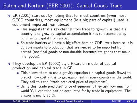
Eaton and Kortum (EER 2001): Capital Goods Trade

EK (2001) start out by noting that for most countries (even mostOECD countries), most equipment (ie a big part of capital) used isequipment imported from abroad.

This suggests that a key channel from trade to ‘growth’ is that if acountry is to grow by capital accumulation it has to accumulate bypurchasing capital from abroad.So trade barriers will have a big effect here on GDP levels because it isdurable inputs to production that are needed to be imported fromabroad (not final goods or non-durable intermediate goods that makefinal goods).

They develop an EK (2002)-style Ricardian model of capitalproduction and capital trade in GE.

This allows them to use a gravity equation (in capital goods flows) topredict how costly it is to get equipment in every country in the world.They call this the “trade predicted price of equipment”.Using this ‘trade predicted’ price of equipment they ask how much ofworld Y/L variation can be accounted for by trade in equipment. Theanswer is nearly 25 %.


EK (2001): Most countries import equipment

Table 2Trade in manufactures and equipment�

No. Country Imports in absorption Imports from &Big 7'

Manufactures Equipment Manufactures Equipment(%) (%) (%) (%)

1 Australia 25.8 58.0 72.1 81.12 Austria 41.5 62.3 76.5 80.63 Bangladesh 50.8 80.9 36.6 49.04 Canada 31.7 62.6 88.8 91.95 Denmark 57.2 92.0 67.0 78.76 Egypt 33.7 64.6 59.7 79.77 Finland 28.0 57.2 69.4 78.18 France 25.3 40.3 60.4 75.09 Germany 26.1 34.1 49.3 62.5

10 Greece 35.4 67.7 66.4 76.011 Hungary 29.1 53.0 33.0 38.112 India 12.2 24.3 53.6 73.913 Iran 26.6 45.7 55.7 74.314 Italy 29.0 54.9 59.7 73.115 Japan 5.3 4.7 45.8 73.816 Kenya 18.7 60.0 66.1 74.417 Korea 23.1 47.9 80.0 90.018 Malawi 42.4 99.3 44.1 64.419 Mauritius 35.3 87.6 46.3 61.420 Morocco 32.8 66.0 67.3 82.021 New Zealand 30.3 57.1 66.7 75.122 Nigeria 29.1 73.0 66.1 72.723 Norway 41.5 49.9 67.0 77.424 Pakistan 33.3 66.4 64.6 74.425 Philippines 23.5 72.3 57.2 75.826 Portugal 31.1 74.1 64.0 76.827 Spain 16.4 46.0 74.4 84.128 Sri Lanka 48.9 94.0 48.4 72.629 Sweden 41.5 80.5 57.4 70.030 Turkey 22.4 53.2 64.9 75.131 United Kingdom 28.7 46.1 57.2 70.032 United States 11.9 16.6 44.4 58.833 Yugoslavia 15.6 31.4 55.5 63.834 Zimbabwe 18.8 64.7 54.7 72.2

�All data are for 1985. Absorption (the denominator of the import share) is calculated as grossproduction plus imports less exports. Imports from the &Big 7' (France, Germany, Japan, Italy,Sweden, United Kingdom, and United States) are shown as a percentage of total imports. The tradedata are from Feenstra et al. (1997) and the production data are from UNIDO (1999).

1202 J. Eaton, S. Kortum / European Economic Review 45 (2001) 1195}1235


EK (2001): Most countries import equipment

Table 3Sources of equipment purchases�

Importing Source of equipment purchases (% of absorption)country

Home US Japan Germany UK France Italy Sweden

Europe:Austria 37.7 3.2 3.6 33.0 2.7 2.4 3.9 1.5Denmark 8.0 7.9 6.8 28.0 10.3 4.6 4.7 10.2Finland 42.8 4.7 5.7 13.8 5.1 2.7 2.8 10.0France 59.7 7.0 3.2 10.7 3.9 * 4.6 0.9Germany 65.9 5.2 5.1 * 3.6 3.5 3.0 0.9Greece 32.3 3.8 3.8 18.7 5.3 5.2 13.4 1.3Hungary 47.0 1.6 2.1 10.9 1.4 1.6 1.6 1.1Italy 45.1 6.6 3.7 16.6 5.6 6.2 * 1.4Norway 50.1 6.1 3.7 9.9 6.1 2.0 2.3 8.5Portugal 25.9 5.0 5.9 18.8 8.5 7.3 9.3 2.1Spain 54.0 6.5 5.2 10.9 4.2 5.4 5.4 1.2Sweden 19.5 10.3 8.0 20.7 9.4 4.7 3.3 *

Turkey 46.8 7.1 6.7 14.0 4.5 2.0 4.9 0.8UK 53.9 11.0 5.3 8.5 * 3.4 2.8 1.3Yugoslavia 68.6 2.9 0.6 8.2 1.6 1.5 4.0 1.2

Paci"c:Australia 42.0 15.9 16.3 5.5 4.5 1.2 2.1 1.5Canada 37.4 45.7 5.8 2.1 1.8 0.8 0.7 0.6Japan 95.3 2.7 * 0.4 0.2 0.1 0.1 0.1Korea 52.1 12.9 23.9 2.5 1.0 1.5 0.4 0.8New Zealand 42.9 11.6 15.6 4.8 6.7 1.5 1.7 1.0Philippines 27.7 26.0 18.1 5.3 2.2 1.7 0.9 0.5US 83.4 * 6.4 1.3 0.9 0.5 0.4 0.2

South Asia:Bangladesh 19.1 5.7 14.9 6.6 6.7 4.0 1.6 0.3India 75.7 3.7 4.0 4.5 2.9 1.9 0.8 0.3Iran 54.3 0.9 7.2 13.4 4.9 0.9 5.6 1.1Pakistan 33.6 11.5 12.2 9.7 8.5 2.5 3.9 1.2Sri Lanka 6.0 8.9 27.8 10.0 12.9 3.9 2.5 2.2

Africa:Egypt 35.4 10.0 8.0 10.7 5.3 6.3 10.2 0.9Kenya 40.0 4.0 7.4 7.4 17.4 3.3 3.7 1.4Malawi 0.7 8.0 5.6 7.0 26.9 8.7 6.3 1.3Mauritius 12.4 1.2 12.0 5.3 8.4 23.3 3.2 0.3Morocco 34.0 3.2 2.7 7.5 3.7 27.7 7.0 2.4Nigeria 27.0 8.1 8.0 8.8 16.7 5.5 5.5 0.5Zimbabwe 35.3 9.1 2.3 7.0 14.7 4.9 6.7 2.1

�All data are for 1985. Absorption of equipment is calculated as gross production of equipment-producing industries plus imports less exports. The trade data are from Feenstra et al. (1997) and theproduction data are from UNIDO (1999).

1204 J. Eaton, S. Kortum / European Economic Review 45 (2001) 1195}1235


EK (2001) meets Hseih and Klenow (AER, 2007)

HK (2007) cast doubt on the details of the EK (2001) mechanism.

They argue that if EK (2001) were right, then the price of equipmentwould be much higher in poor countries.

EK (2001)’s Figure 6 plots just this: the observed price of equipment(from the International Comparison of Prices (ICP) project).

EK’s reply would (presumably) be: We don’t really believe this ICPdata. Such data is very hard to collect. Our ‘trade predicted’equipment price (which is derived from the choices that firms in poorcountries make about whether to buy capital from home or fromGermany) is what we believe.


EK (2001): ICP Equipment Price Data

Fig. 6. Development and the price of equipment.

�� The variability across countries in the price of equipment is certainly consistent with theexistence of large trade costs. Heston et al. (1995) examine this variability in ICP prices in moredetail. In particular, they look at how cross-country variability in the price structure di!ers betweengoods that are tradable and those that are not. Although they "nd a bit less variability in the pricesof the tradable goods, they admit that the law of one price is far from holding among tradables. Theyconclude with a plea for a closer examination of how trade in#uences prices: `The extent andcharacter of a country's international trade certainly a!ects the price structure of its tradables versusthat of its nontradables, and this is a prime area to focus on.a We hope to be pushing in thatdirection here.

price of investment itself that is relevant for deciding where to buy equipment.The last two columns of Table 4 present both the denominator and numeratorof the relative price of equipment as measured by the ICP. While the relativeprice of equipment is substantially lower in richer countries, the reported priceof equipment itself is, if anything, higher in such countries (Fig. 6 illustrates).The ICP measure of equipment prices certainly varies across countries, but thenumbers do not show that it is systematically higher in the net importers thanin the net exporters of equipment. This last result is surprising: Home-bias andregionalism suggest that geographic barriers in capital goods trade are substan-tial, which would normally imply lower prices in exporting countries.��

We can summarize our discussion so far with seven apparent facts extractedfrom various data sources:

1. According to production data, a small group of R&D intensive countries arethe most specialized in equipment production.

J. Eaton, S. Kortum / European Economic Review 45 (2001) 1195}1235 1207


Intermediate Input Trade

There has been a lot of recent work on this. One source of confusionis whether we want to include cheaper intermediate inputs as part of‘productivity’ or simply as something that raises Y/L.

Broad, Greenfield and Weinstein (2006):

Estimate the ‘productivity’ effects inherent in a Romer-style productionfunction (which features ‘love of variety’, a la Dixit-Stiglitz).They make the assumption that if the same ‘good’ (eg groundnuts) isavailable from country A and country B, then these are differentvarieties of the good.They quantify the productivity benefits of all the new ‘varieties’ thatLDCs have been importing around the world between 1994 and 2003.Quantifying the gains from new varieties requires: CES assumption,estimate of the CES parameter, and the Sato-Vartia-Feenstra formula.(See Feenstra (AER, 1994)).This accounts for 15 % of productivity growth over the period.


Intermediate Input Trade

Amiti and Konings (AER, 2007):

Focus on the trade liberalization (lower tariffs) effects of cheaperimported intermediate goods for domestic firms. (Recall, most of thesefirm-level trade liberalization studies focus on how tariffs change theprices of the final goods in which firms compete.)

This takes seriously Corden’s old idea of “effective protection” (that animport-competing firm enjoys protection on its output good but suffersfrom protection on its input goods, so the appropriate measure of acountry’s level of protection should take both of these forces intoaccount).

The effects are large: about twice as large as those coming aboutthrough output goods tariffs.

Other important recent work by Goldberg, Khandelwal, Pavcnik andTopalova (QJE 2010).



Brief introduction.






Does technology embodied in physical goods (intermediate inputs orcapital equipment) lead to important international technology?transfer?




Endogenous Growth: Other Effects

There is not much work on these in a specifically international setting.

Market Size Effect:

But Acemoglu and Lin (QJE, 2003) does this domestically, using‘market size’ for pharmaceuticals generated by demographic change.Sokoloff (JEH, 1998) looks at innovation (patenting) around canals inthe early 19th century United States.Trefler and Lileeva (QJE 2010) and Bustos (AER 2010) potentially fitunder this heading, though the meachanisms at work are different.

Competition Effect:

Aghion, Bloom, Blundell, Griffith and van Reenen (QJE 2007) is a nicestudy of competition and innovation (patenting) in the UK. Some oftheir exogenous competition ‘shock’ variables relate to importcompetition.Some work surveyed in Tybout (Handbook chapter, 2001) can beinterpreted in this way.


Other Trade and Growth Channels

Institutional Change:

Acemoglu, Johnson and Robinson (AER, 2005): Gains from “AtlanticTrade” around the industrial revolution are too big to be gains fromtrade. Likely that trade openness changed domestic institutions for thebetter.Levchenko (ReStud 2007) formalized this notion.

Learning by Doing:

Very little work on this in general.Irwin and Klenow (JPE 1994) looks at LBD in the semiconductorindustry. Finds some evidence of learning both from both domesticproduction and foreign (other firms’) production.Irwin (JEH, 2000) is study of the US tinplate industry.Benkard (AER 2000) is purely domestic study of US airline industry.Thornton and Thompson (AER 2001) is purely domestic LBD study of‘liberty ship’ building in US.


14.581 international trade lecture 20: trade and growth...

Documents