14.581 international trade š lecture 14: firm ... · pdf fileš lecture 14: firm...

14.581 International Trade Lecture 14: Firm Heterogeneity Theory (I)

Melitz (2003)

14.581

Week 8

Spring 2013

14.581 (Week 8) Melitz (2003) Spring 2013 1 / 42

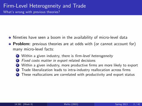
Firm-Level Heterogeneity and TradeWhats wrong with previous theories?

Nineties have seen a boom in the availability of micro-level data

Problem: previous theories are at odds with (or cannot account for)many micro-level facts:

1 Within a given industry, there is rm-level heterogeneity2 Fixed costs matter in export related decisions3 Within a given industry, more productive rms are more likely to export4 Trade liberalization leads to intra-industry reallocation across rms5 These reallocations are correlated with productivity and export status


Firm-Level Heterogeneity and TradeWhat does Melitz (2003) do about it?

Melitz (2003) will develop a model featuring facts 1 and 2 that canexplain facts 3, 4, and 5

This is by far the most inuential trade paper in the last 10 years

Two building blocks:1 Krugman (1980): CES, IRS technology, monopolistic competition2 Hopenhayn (1992): equilibrium model of entry and exit

From a normative point of view, Melitz (2003) may also providenewsource of gains from trade if trade induces reallocation of laborfrom least to most productive rms (more on that later)


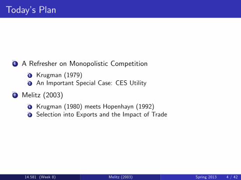
Todays Plan

1 A Refresher on Monopolistic Competition

1 Krugman (1979)2 An Important Special Case: CES Utility

2 Melitz (2003)

1 Krugman (1980) meets Hopenhayn (1992)2 Selection into Exports and the Impact of Trade


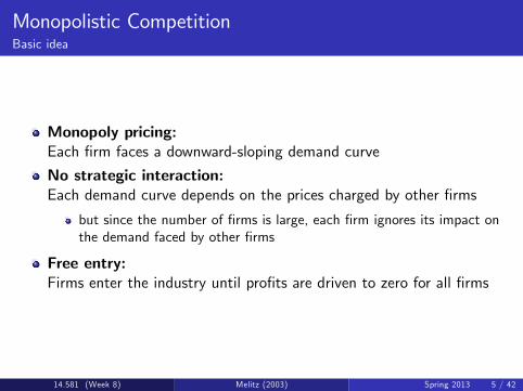
Monopolistic CompetitionBasic idea

Monopoly pricing:Each rm faces a downward-sloping demand curve

No strategic interaction:Each demand curve depends on the prices charged by other rms

but since the number of rms is large, each rm ignores its impact onthe demand faced by other rms

Free entry:Firms enter the industry until prots are driven to zero for all rms


Monopolistic CompetitionGraphical analysis

MR

q

p AC

MC

D


Krugman (1979)Endowments, preferences, and technology

Endowments: All agents are endowed with 1 unit of laborPreferences: All agents have the same utility function given by

U =R n0 u (ci ) di

where:

u (0) = 0, u0 > 0, and u00 < 0 (love of variety)σ (c) u 0

cu 00 > 0 is such that σ0 0 (why?)

IRS Technology: Labor used in the production of each variety is

li = f + qi/ϕ

where ϕ common productivity parameter


Krugman (1979)Equilibrium conditions

1 Consumer maximization:

pi = λ1u0 (ci )

2 Prot maximization:

pi =

σ (ci )σ (ci ) 1

wϕ

3 Free entry:

pi wϕ

qi = wf

4 Good and labor market clearing:

qi = Lci

L = nf +R n0qiϕdi


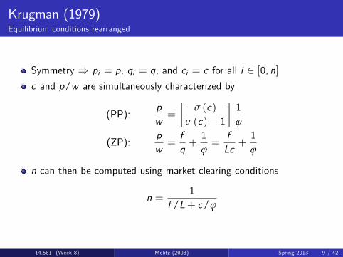
Krugman (1979)Equilibrium conditions rearranged

Symmetry ) pi = p, qi = q, and ci = c for all i 2 [0, n]c and p/w are simultaneously characterized by

(PP):pw=

σ (c)

σ (c) 1

1ϕ

(ZP):pw=fq+1ϕ=fLc+1ϕ

n can then be computed using market clearing conditions

n =1

f /L+ c/ϕ


Krugman (1979)Graphical analysis

(p/w)0

c0

Z

c

p/wP

PZ


Krugman (1979)Gains from trade revisited

(p/w)0

c1 c0

Z’

Z

c

p/wP

Z’

PZ(p/w)1

Suppose that two identical countries open up to trade

This is equivalent to a doubling of country size (which would have noe¤ect in a neoclassical trade model)

Because of IRS, opening up to trade now leads to:

Increased product variety: c1 < c0 ) 1f /2L+c1/ϕ >

1f /L+c0/ϕ

Pro-competitive/e¢ ciency e¤ects: (p/w)1 < (p/w)0 ) q1 > q0


CES UtilityTrade economistsmost preferred demand system

Constant Elasticity of Substitution (CES) utility corresponds to thecase where:

U =R n0 (ci )

σ1σ di ,

where σ > 1 is the elasticity of substitution between pair of varieties

This is the case considered in Krugman (1980)

What is it to like about CES utility?

Homotheticity (u (c) (c)σ1

σ is actually the only functional formsuch that U is homothetic)Can be derived from discrete choice model with i.i.d extreme valueshocks (See Feenstra Appendix B)

Is it empirically reasonable?


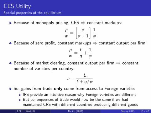
CES UtilitySpecial properties of the equilibrium

Because of monopoly pricing, CES ) constant markups:

pw=

σ

σ 1

1ϕ

Because of zero prot, constant markups ) constant output per rm:

pw=fq+1ϕ

Because of market clearing, constant output per rm ) constantnumber of varieties per country:

n =L

f + q/ϕ

So, gains from trade only come from access to Foreign varietiesIRS provide an intuitive reason why Foreign varieties are di¤erentBut consequences of trade would now be the same if we hadmaintained CRS with di¤erent countries producing di¤erent goods


CES UtilitySpecial properties of the equilibrium

Decentralized equilibrium is e¢ cientDecentralized equilibrium solves:

maxqi ,n

R n0 pi (qi ) qidi

subject to : nf +R n0qiϕdi L.

A central planner would solve:

maxqi ,n

R n0 (qi )

σ1σ di

subject to: nf +R n0qiϕdi L.

Under CES, pi (qi ) qi ∝ q11σ

i ) Two solutions coincideThis is unique to CES (in general, entry is distorted)This implies that many properties of perfectly competitive models willcarry over to this environment


Melitz (2003)Demand

Like in Krugman (1980), representative agent has CES preferences:

U =Z

ω2Ωq (ω)

σ1σ dω

σσ1

where σ > 1 is the elasticity of substitutionConsumption and expenditures for each variety are given by

q (ω) = Qp (ω)P

σ

(1)

r (ω) = Rp (ω)P

1σ

(2)

where:

P Z

ω2Ωp (ω)1σ dω

11σ

, R Z

ω2Ωr (ω) , and Q R/P


Melitz (2003)Production

Like in Krugman (1980), labor is the only factor of productionL total endowment, w = 1 wage

Like in Krugman (1980), there are IRS in production

l = f + q/ϕ (3)

Like in Krugman (1980), monopolistic competition implies

p (ϕ) =1

ρϕ(4)

CES preferences with monopoly pricing, (2) and (4), imply

r (ϕ) = R (Pρϕ)σ1 (5)

These two assumptions, (3) and (4), further imply

π (ϕ) r (ϕ) l (ϕ) = r (ϕ)σ

f



Comments:1 Higher productivity ϕ in the model implies higher measured productivity

r(ϕ)l (ϕ)

=1ρ

1 f

l (ϕ)

2 More productive rms produce more and earn higher revenues

q (ϕ1)q (ϕ2)

=

ϕ1ϕ2

σ

andr (ϕ1)r (ϕ2)

=

ϕ1ϕ2

σ1

3 ϕ can also be interpreted in terms of quality. This is isomorphic to achange in units of account, which would a¤ect prices, but nothing else


Melitz (2003)Aggregation

By denition, the CES price index is given by

P =Z

ω2Ωp (ω)1σ dω

11σ

Since all rms with productivity ϕ charge the same price p (ϕ), wecan rearrange CES price index as

P =Z +∞

0p (ϕ)1σMµ (ϕ) dϕ

11σ

where:

M mass of (surviving) rms in equilibriumµ (ϕ) (conditional) pdf of rm-productivity levels in equilibrium



Combining the previous expression with monopoly pricing (4), we get

P = M11σ /ρeϕ

where

eϕ Z +∞

0ϕσ1µ (ϕ) dϕ

1σ1

One can do the same for all aggregate variables

R = Mr (eϕ) , Π = Mπ (eϕ) , Q = M σσ1 q (eϕ)

Comments:1 These are the same aggregate variables we would get in a Krugman(1980) model with a mass M of identical rms with productivity eϕ

2 But productivity eϕ now is an endogenous variable which may respondto changes in trade cost, leading to aggregate productivity changes


Melitz (2003)Entry and exit

In order to determine how µ (ϕ) and eϕ get determine in equilibrium,one needs to specify the entry and exit of rms

Timing is similar to Hopenhayn (1992):1 There is a large pool of identical potential entrants deciding whether tobecome active or not

2 Firms deciding to become active pay a xed cost of entry fe > 0 andget a productivity draw ϕ from a cdf G

3 After observing their productivity draws, rms decide whether toremain active or not

4 Firms deciding to remain active exit with a constant probability δ


Melitz (2003)Aside: Pareto distributions

In variations and extensions of Melitz (2003), most commonassumption on the productivity distribution G is Pareto:

G (ϕ) 1

ϕ

ϕ

θ

for ϕ ϕ

g (ϕ) θϕθ ϕθ1 for ϕ ϕ

Pareto distributions have two advantages:1 Combined with CES, it delivers closed form solutions2 Distribution of rm sizes remains Pareto, which is not a badapproximation empirically (at least for the upper tail)

But like CES, Pareto distributions will have very strong implicationsfor equilibrium properties (more on this later)


Melitz (2003)Productivity cuto¤

In a stationary equilibrium, a rm either exits immediately or producesand earns the same prots π (ϕ) in each period

In the absence of time discounting, expected value of a rm withproductivity ϕ is

v (ϕ) = max0,∑+∞

t=0 (1 δ)t π (ϕ)= max

0,

π (ϕ)

δ

There exists a unique productivity level ϕ inf

nϕ 0 : π(ϕ)

δ > 0o

Productivity cuto¤ ϕ can also be written as:

π (ϕ) = 0


Melitz (2003)Aggregate productivity

Once we know ϕ, we can compute the pdf of rm-productivity levels

µ (ϕ) =

(g (ϕ)

1G (ϕ) if ϕ ϕ

0 if ϕ < ϕ

Accordingly, the measure of aggregate productivity is given by

eϕ (ϕ) = 11 G (ϕ)

Z +∞

ϕϕσ1g (ϕ) dϕ

1σ1


Melitz (2003)Free entry condition

Let π Π/M denote average prots per period for surviving rms

Free entry requires the total expected value of prots to be equal tothe xed cost of entry

0 G (ϕ) + π

δ [1 G (ϕ)] = fe

Free Entry Condition (FE):

π =δfe

1 G (ϕ) (6)

Holding constant the xed costs of entry, if rms are less likely tosurvive, they need to be compensated by higher average prots


Melitz (2003)Zero cuto¤ prot condition

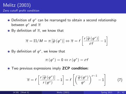
Denition of ϕ can be rearranged to obtain a second relationshipbetween ϕ and π

By denition of π, we know that

π = Π/M = π [eϕ (ϕ)], π = fr [eϕ (ϕ)]

σf 1

By denition of ϕ, we know that

π (ϕ) = 0, r (ϕ) = σf

Two previous expressions imply ZCP condition:

π = fr [eϕ (ϕ)]r (ϕ)

1= f

"eϕ (ϕ)ϕ

σ1 1

#(7)


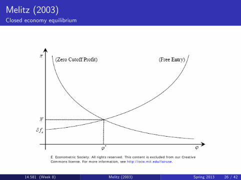
Melitz (2003)Closed economy equilibrium


É Econometric Society. All rights reserved. This content is excluded from our CreativeCommons license. For more information, see http://ocw.mit.edu/fairuse.

http://ocw.mit.edu/fairuse

Melitz (2003)Aside: the shape of the ZCP schedule

FE and ZCP, (6) and (7), determine a unique (π, ϕ), and thereforeeϕ, independently of country size Lthe only variable left to compute is M, which can be done using freeentry and labor market clearing as in Krugman (1980)

However, ZCP is not necessarily downward sloping:

it depends on whether eϕ or ϕ increases relatively fasterZCP is downward sloping for most common distributions

In the Pareto case, it is easy to check that eϕ/ϕ is constant:

So ZCP is at and average prots are independent of ϕ


Melitz (2003)Number of varieties and welfare

Free entry and labor market clearing imply

L = R = rM

We can rearrange the previous expression

M =Lr=

Lσ (π + f )

Like in Krugman (1980), welfare of a representative worker is given by

U = 1/P = M1

σ1 ρeϕSince eϕ and π are independent of L, growth in country size andcostless trade will also have the same impact as in Krugman (1980):

welfare % because of % in total number of varieties in each country


Melitz (2003)Open economy model

In the absence of trade costs, we have seen trade integration does notlead to any intra-industry reallocation (eϕ is xed)In order to move away from such (counterfactual) predictions, Melitz(2003) introduces two types of trade costs:

1 Iceberg trade costs: in order to sell 1 unit abroad, rms need to shipτ 1 units

2 Fixed exporting costs: in order to export abroad, rms must incur anadditional xed cost fex (information, distribution, or regulation costs)after learning their productivity ϕ

In addition, Melitz (2003) assumes that c = 1, ..., n countries aresymmetric so that wc = 1 in all countries



Monopoly pricing now implies

pd (ϕ) =1

ρϕ, px (ϕ) =

τ

ρϕ

Revenues in the domestic and export markets are

rd (ϕ) = Rd [Pdρϕ]σ1 , rx (ϕ) = τ1σRx [Pxρϕ]σ1

Note that by symmetry, we must have

Pd = Px = P and Rd = Rx = R

Let fx δfex . Prots in the domestic and export markets are

πd (ϕ) =rd (ϕ)

σ f , πx (ϕ) =

rx (ϕ)σ

fx


Melitz (2003)Productivity cuto¤s

Expected value of a rm with productivity ϕ is

v (ϕ) = max0,∑+∞

t=0 (1 δ)t π (ϕ)= max

0,

π (ϕ)

δ

But total prots of are now given by

π (ϕ) = πd (ϕ) +max f0,πx (ϕ)g

Like in the closed economy, we let ϕ infn

ϕ 0 : π(ϕ)δ > 0

oIn addition, we let ϕx inf

nϕ ϕ : πx (ϕ)

δ > 0obe the export

cuto¤In order to have both exporters and non-exporters in equilibrium,ϕx > ϕ, we assume that:

τσ1fx > f


Melitz (2003)Selection into exports


Exit Don’t Export Export

-fD

0

π

-fX

(ϕ*)σ−1 (ϕx)σ−1*

(ϕ)σ−1

πD

πX

Image by MIT OpenCourseWare.

Melitz (2003)Are exporters more productive than non-exporters?

In the model, more productive rms (higher ϕ) select into exports

Empirically, this directly implies larger rms (higher r (ϕ))

Question: Does that also mean that rms with higher measuredproductivity select into exports?

Answer: Yes. For this to be true, we need

rd (ϕ) + nrx (ϕ)ld (ϕ) + nlx (ϕ)

>rd (ϕ)ld (ϕ)

,

which always holds if τσ1fx > f

Comment: Like in the closed economy, this crucially relies on thefact that xed labor costs enter the denominator



In the open economy, aggregate productivity is now given by

eϕt = 1Mt

hMeϕσ1 + nMx (eϕx/τ)σ1

i 1σ1

where:

Mt M + nMx is the total number of varieties

eϕ = 11G (ϕ)

Z +∞

ϕϕσ1g (ϕ) dϕ

1σ1

is the average productivity

across all rms

eϕx = 11G (ϕx )

Z +∞

ϕxϕσ1g (ϕ) dϕ

1σ1

is the average productivity

across all exporters



Once we know eϕt , we can still compute all aggregate variables as:P = M

11σt /ρeϕt ,

R = Mt r (eϕt ) ,Π = Mtπ (eϕt ) ,Q = M

σσ1t q (eϕt )

Comment:

Like in the closed economy, there is a tight connection between welfare(1/P) and average productivity (eϕt )But in the open economy, this connection heavily relies on symmetry:welfare depends on the productivity of foreign, not domestic exporters


Melitz (2003)Free entry condition

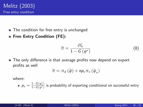
The condition for free entry is unchanged

Free Entry Condition (FE):

π =δfe

1 G (ϕ) (8)

The only di¤erence is that average prots now depend on exportprots as well

π = πd (eϕ) + npxπx (eϕx )where:

px =1G (ϕx )1G (ϕ) is probability of exporting conditional on successful entry


Melitz (2003)Zero cuto¤ prot condition

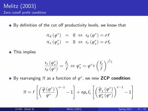
By denition of the cut o¤ productivity levels, we know that

πd (ϕ) = 0 , rd (ϕ

) = σf

πx (ϕx ) = 0 , rx (ϕx ) = σfx

This implies

rx (ϕx )rd (ϕ)

=fxf, ϕx = ϕτ

fxf

1σ1

By rearranging π as a function of ϕ, we new ZCP condition:

π = f

"eϕ (ϕ)ϕ

σ1 1

#+ npx fx

"eϕx (ϕ)ϕx (ϕ

)

σ1 1

#


Melitz (2003)The Impact of Trade


π

δfa

ϕa ϕ ϕ

Free entry

Trade

Autarky

Zero cutoff profit

π_

πa_



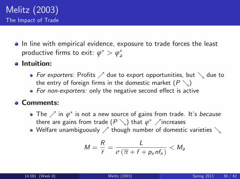
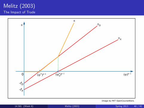
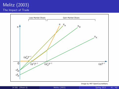
In line with empirical evidence, exposure to trade forces the leastproductive rms to exit: ϕ > ϕaIntuition:

For exporters: Prots % due to export opportunities, but & due tothe entry of foreign rms in the domestic market (P &)For non-exporters: only the negative second e¤ect is active

Comments:

The % in ϕ is not a new source of gains from trade. Its becausethere are gains from trade (P &) that ϕ %increasesWelfare unambiguously % though number of domestic varieties &

M =Rr=

Lσ (π + f + pxnfx )

< Ma




-fD

0

-fX

(ϕ*)σ−1 (ϕx)σ−1*

πD

ππ

πX

(ϕ)σ−1




-fD

0

π

-fX

(ϕa)σ−1

πDπaπ

πX

*

(ϕ∗)σ−1 (ϕ)σ−1(ϕx)σ−1∗

Lose Market Share Gain Market Share


Melitz (2003)Other comparative static exercises

Starting from autarky and moving to trade is theoretically standard,but not empirically appealing

Melitz (2003) also considers:1 Increase in the number of trading partners n2 Decrease in iceberg trade costs τ3 Decrease in xed exporting costs fx

Same qualitative insights in all scenarios:

Exit of least e¢ cient rmsReallocation of market shares from less from more productive rmsWelfare gains


MIT OpenCourseWarehttp://ocw.mit.edu

14.581 International Economics ISpring 2013

For information about citing these materials or our Terms of Use, visit: http://ocw.mit.edu/terms.

http://ocw.mit.edu

http://ocw.mit.edu/terms.

14.581 international trade š lecture 14: firm ... · pdf fileš lecture 14: firm...

Documents