14.581 international trade — — | lecture 25: trade ... · explaining trade policy gawande and...

— —

14.581

Spring 2013

14.581 Trade Policy Empirics Spring 2013 1 / 19

14.581 International Trade— Lecture 25: Trade Policy Empirics (I) —

14.581

Spring 2013

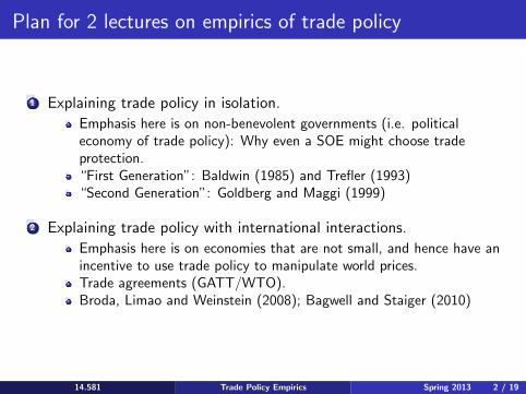
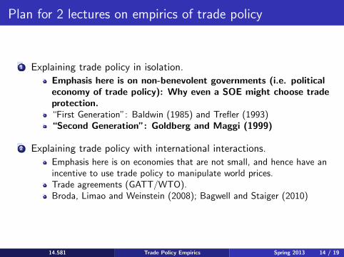
Plan for 2 lectures on empirics of trade policy

1 Explaining trade policy in isolation. Emphasis here is on non-benevolent governments (i.e. political economy of trade policy): Why even a SOE might choose trade protection. “First Generation”: Baldwin (1985) and Trefler (1993) “Second Generation”: Goldberg and Maggi (1999)

2 Explaining trade policy with international interactions. Emphasis here is on economies that are not small, and hence have an incentive to use trade policy to manipulate world prices. Trade agreements (GATT/WTO). Broda, Limao and Weinstein (2008); Bagwell and Staiger (2010)


Explaining Trade Policy

Gawande and Krishna (Handbook chapter, 2003) have a nice survey of this literature.

“If, by an overwhelming consensus among economists, trade should be free, then why is it that nearly everywhere we look, and however far back, trade is in chains?”

One answer: even in a neoclassical economy, trade policy might be optimal for a non-SOE. (Broda, Limao and Weinstein (2008) have recently improved support for this claim, as we will discuss later). Another answer: we live in an imperfectly competitive world where it is possible that even a SOE would want import tariffs/export subsidies. (Helpman and Krugman, 1987 book). Political economy answer: governments don’t maximize social welfare.


Gawande and Krishna (2003) Survey

Divide empirical work on ‘explaining trade policy’ into two epochs: 1

2

“First generation”: pre-Grossman and Helpman (1994) “Second generation”: post-GH (1994).

Nice example of the importance of theory for doing good empirical work in Trade.



1

2

Explaining trade policy in isolation. Emphasis here is on non-benevolent governments (i.e. political economy of trade policy): Why even a SOE might choose trade protection. “First Generation”: Baldwin (1985) and Trefler (1993) “Second Generation”: Goldberg and Maggi (1999)

Explaining trade policy with international interactions. Emphasis here is on economies that are not small, and hence have an incentive to use trade policy to manipulate world prices. Trade agreements (GATT/WTO). Broda, Limao and Weinstein (2008); Bagwell and Staiger (2010)


“First Generation” Empirical work I

This body of work was impressive and large, but it always suffered from a lack of strong theoretical input that would suggest:

What regression to run. What the coefficients in a regression would be telling us. What endogeneity problems seem particulary worth worrying about.


“First Generation” Empirical work II

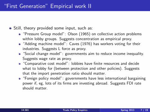
Still, theory provided some input, such as: “Pressure Group model”: Olson (1965) on collective action problems within lobby groups. Suggests concentration as empirical proxy. “Adding machine model”: Caves (1976) has workers voting for their industries. Suggests L force as proxy. “Social change model”: governments aim to reduce income inequality. Suggests wage rate as proxy. “Comparative cost model”: lobbies have finite resources and decide what to lobby for (between protection and other policies). Suggests that the import penetration ratio should matter. “Foreign policy model”: governments have less international bargaining power if, eg, lots of its firms are investing abroad. Suggests FDI rate should matter.


Trefler (JPE 1993)

Trefler (1993) conducts a similar empirical exercise to Baldwin (1985), but for:

Focus on ‘NTB coverage ratios’ (the proportion of imports in an industry that are subject to any sort of NTB) rather than tariffs. This is attractive since US tariffs are so low in this period that there isn’t much variation. Also true that tariffs (being under the remit of GATT/WTO) are constrained by international agreements in a way that NTBs are not. Attention to endogeneity issues and specification issues:

Simultaneity: Protection depends on import penetration ratio (IPR) but IPR depends on protection. Truncation: IPR can’t go negative. NTB coverage ratio can’t go negative.


Trefler (1993)

Trefler (1993) estimates the following system by FIML:

Where N∗ = MγM + XN βN + εN , M∗ = NγN + XM βM + εM , N is the NTB coverage ratio and M is the import penetration ratio.

XN is Baldwin (1985) style variables explaining protection.

XM is H-O style variable explaining trade flows.


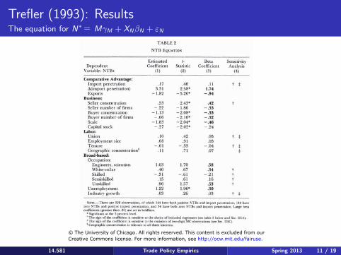
Trefler (1993): ResultsThe equation for N ∗ MγM + XNβN + εN


© The University of Chicago. All rights reserved. This content is excluded from ourCreative Commons license. For more information, see http://ocw.mit.edu/fairuse.

=

http://ocw.mit.edu/fairuse

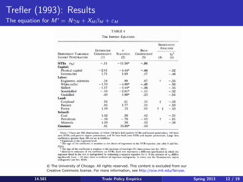
Trefler (1993): ResultsThe equation for M ∗ NγN + XMβM + εM

B. The Import Equation 14.581 Trade Policy Empirics Spring 2013 12 / 19


=

=


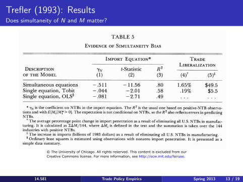
Trefler (1993): Results Does simultaneity of N and M matter?

150 JOURNAL OF POLITICAL ECONOMY

TABLE 5

EVIDENCE OF SIMULTANEITY BIAS

IMPORT EQUATION* TRADE

2 LIBERALIZATION DESCRIPTION 'YN t-Statistic R L

OF THE MODEL (1) (2) (3) (4)' (5)1

Simultaneous equations - .511 - 11.56 .80 1.65% $49.5 Single equation, Tobit -.044 -2.01 .58 .19% $5.5 Single equation, OLS? -.081 -2.71 .49 ... ...

* YN is the coefficient on NTBs in the import equation. The R2 is the usual one based on positive-NTB observations and with E[MiIM > 0]. The expectation is not conditional on NTBs, so the R 2 also reflects errors in predicting NTBs.

* The average percentage point change in import penetration as a result of eliminating all U.S. NTBs in manufacturing. It is calculated as XAMi/144, where AM, is defined in the text and the summation is taken over the 144 industries with positive NTBs.

The increase in imports (billions of 1983 dollars) as a result of eliminating all U.S. NTBs in manufacturing. Ordinary least squares is estimated using observations with nonzero import penetration. It is presented as a

simple data summary.

equations t-statistic is very large and the R2 has risen to .80. This is indicative of simultaneity bias. Indeed, with the Hausman (1978)





1

2

Explaining trade policy in isolation. Emphasis here is on non-benevolent governments (i.e. political economy of trade policy): Why even a SOE might choose trade protection. “First Generation”: Baldwin (1985) and Trefler (1993) “Second Generation”: Goldberg and Maggi (1999)

Explaining trade policy with international interactions. Emphasis here is on economies that are not small, and hence have an incentive to use trade policy to manipulate world prices. Trade agreements (GATT/WTO). Broda, Limao and Weinstein (2008); Bagwell and Staiger (2010)


“Second Generation” Empirical Work

Grossman and Helpman (‘Protection for Sale’, AER 1994) provided a clean theoretical ‘GE’ (the economy is not really GE, but the lobbying of one industry does affect the lobbying of another) model that delivered an equation for industry-level equilibrium protection as a function of industry-level observables: � � � �

ti 1 + ti

= − αL

a + αL

zi ei

+ 1

a + αL Ii ×

zi ei

. (1)

Where: ti is the ad valorem tariff rate in industry i . Ii is a dummy for whether industry i is organized or not. 0 ≤ αL ≤ 1 is the share of the population that is organized into lobbies. a > 0 is the weight that the government puts on social welfare relative to aggregate political contributions (whose weight is 1). zi is the inverse import penetration ratio. ei is the elasticity of import demand.


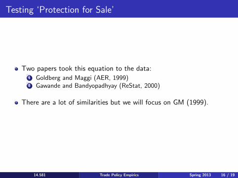
Testing ‘Protection for Sale’

Two papers took this equation to the data: 1

2

Goldberg and Maggi (AER, 1999) Gawande and Bandyopadhyay (ReStat, 2000)

There are a lot of similarities but we will focus on GM (1999).


Goldberg and Maggi (1999)

There a host of key challenges in taking the GH (1994) equation to the data:

How to measure ti ? Ideally want NTBs (not set cooperatively under GATT/WTO) measured in tariff equivalents. Absent this GM (1999) use coverage ratios, as in Trefler (1993). They experiment with different proportionality constants (1/µ) between coverage ratios and t and also correct for censoring of coverage ratios.

Data on ei is obviously hard to get. GM (1999) use existing estimates but also consider them as measured with error, so GM (1999) take ei over to the LHS.


Goldberg and Maggi (1999)

More challenges: How to measure Ii ? Can get data on total political contributions in the US by industry (by law these are supposed to be reported), but all ‘industries’ have at least some contributions, so all seem ‘organized’. GM (1999) experiment with different cutoffs in this variable. This isn’t innocuous since contributions are endogenous in the GH (1994) model. GM (1999) use as instruments for Ii a set of typical Baldwin (1985)-style regressors, ie Trefler’s N equation.

zi is endogenous (as Trefler (1993) highlighted). GM (1999) use Trefler-style instruments for zi (Trefler’s M equation).


GM (1999): Results MLE estimates.

AND MAGGI: PROTECTION FOR SALE 1145

size,

not the them in

results with the

In Ta- the posi-

TABLE 1-RESULTS FROM THE BASIC SPECIFICATION

(G-H MODEL)

Variable ,U = 1 ,U = 2 3

X?IMj -0.0093 -0.0133 -0.0155 (0.0040) (0.0059) (0.0070)

(Xi/Mi) * I 0.0106 0.0155 0.0186 (0.0053) (0.0077) (0.0093)

Implied (3 0.986 0.984 0.981 (0.005) (0.007) (0.009)

Implied aL 0.883 0.858 0.840 (0.223) (0.217) (0.214)

residual in (4) and a predetermined set of ex- planatory variables. Our previous discussion 14.581 Trade Policy Empirics Spring 2013 19 / 19

Courtesy of Pinelopi Koujianou Goldberg, Giovanni Maggi and the American Economic Association. Used with permission.

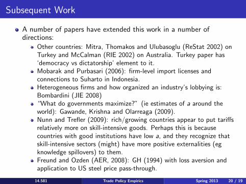
Subsequent Work

A number of papers have extended this work in a number of directions:

Other countries: Mitra, Thomakos and Ulubasoglu (ReStat 2002) on Turkey and McCalman (RIE 2002) on Australia. Turkey paper has ‘democracy vs dictatorship’ element to it. Mobarak and Purbasari (2006): firm-level import licenses and connections to Suharto in Indonesia. Heterogeneous firms and how organized an industry’s lobbying is: Bombardini (JIE 2008) “What do governments maximize?” (ie estimates of a around the world): Gawande, Krishna and Olarreaga (2009). Nunn and Trefler (2009): rich/growing countries appear to put tariffs relatively more on skill-intensive goods. Perhaps this is because countries with good institutions have low a, and they recognize that skill-intensive sectors (might) have more positive externalities (eg knowledge spillovers) to them. Freund and Ozden (AER, 2008): GH (1994) with loss aversion and application to US steel price pass-through.


MIT OpenCourseWarehttp://ocw.mit.edu

14.581 International Economics ISpring 2013

For information about citing these materials or our Terms of Use, visit: http://ocw.mit.edu/terms.

http://ocw.mit.edu

http://ocw.mit.edu/terms.

14.581 international trade — — | lecture 25: trade ... · explaining trade policy gawande and...

Documents