COVER SHEET

This is the author version of article published as: Higgins, A. and Ferreira, Luis and Kozan, Erhan (1996) Optimisation of train schedules to achieve minimum transit times and maximum reliability. In Proceedings 13th International Symposium on Transportation and Traffic Theory, Lyon, France. Copyright 1996 Elsevier Accessed from http://eprints.qut.edu.au

Higgins, A., Ferreira, L. and Kozan, E. (1996). “Optimisation of train schedules to achieve minimum transit times and maximum reliability”, Proceedings of the 13th International Symposium on Transportation and Traffic Theory, 589 - 614.

31

OPTIMISATION OF TRAIN TIMETABLES TO

ACHIEVE MINIMUM TRANSIT TIMES AND

MAXIMUM RELIABILITY Andrew Higgins, Luis Ferreira and Erhan Kozan

ABSTRACT

The overall timetable reliability is a measure of the likely performance of the timetable as a whole, in terms of schedule adherence. The concept is a critical performance measure for both urban and non-urban rail passenger services, as well as rail freight transportation. This paper deals with the scheduling of trains on single track corridors, so as to minimise train trip times and maximise reliability of train arrival times. A method used to quantify the amount of risk of delay associated with each train, each track segment, and the schedule as a whole, is used as the reliability component of the constrained optimisation model. The methodology used to estimate the risk of delay is put forward. The paper also describes a number of alternative solution techniques for the scheduling problem. These techniques include exact optimal solutions using branch and bound, and heuristic approaches, such as genetic algorithms, nearest neighbourhood heuristic and tabu search. Some of the results of using these alternative approaches are briefly described. The schedule produced using risk of delay in the objective function, will be the most efficient in terms of delay due to train conflicts and delay that may occur due to unexpected events. The model and solution techniques are applied to the problem of determining improved positions of sidings on a single track corridor, with respect to a given schedule.

2

INTRODUCTION Efficient train scheduling is designed to achieve a given level of customer service whilst minimising overall train operating costs. Customer service in this context is made up of several attributes which include overall journey time, punctuality and reliability of train arrivals. Transit time reliability is a function of a range of factors, namely: the degree of 'slackness' built into the schedule; the number and position of train conflicts; priorities for each train; station dwell times; and train speeds are all influencing variables. This paper combines a risk of delay model developed by Higgins et al. (1995b), with optimal and heuristic techniques so as to give the optimal/near optimal schedule with respect to train trip times and reliability. The best schedule with respect to minimal train trip time alone, will give the most efficient schedule if there are no unexpected delays to trains. Since this is not the case in practice, a schedule optimised with respect to delay may have a large amount of risk of delays. The objective function presented in this paper is minimised with respect to two components, namely: conflict delays; and risk of delays. Conflict delay is defined as the time loss due to a train conflict being resolved at a siding, when a crossing or overtaking manoeuvre takes place. Risk of delay is the amount of delay due to unforeseen events. The risk of delay is analysed by categorising it into three components, namely: train, track and terminal related risk of delay. A known distribution of delays for each of these components can be obtained from historical data. The risk of delay to any train is calculated as the delay incurred to the train minus the expected recoverability from that delay. This is the general structure for each of the risk of delay components, although the effect of delay to the trains is different for each of the three components. The next section gives a brief critical overview of past work in the area of single track scheduling optimisation. After formulating the train scheduling optimisation model, the methodology used to estimate the risk of delay is described in detail. The various solution techniques used are highlighted including: optimal solutions, genetic algorithms and tabu search heuristics. Finally, an extension of the model is used to determine improved positions of sidings on a single line track with respect to a resolved schedule. In this case, the track segments become decision variables and the final solution will produce the improved siding positions, as well as the optimal schedule given these siding locations.

3

PAST WORK There is a great deal of literature which deals with scheduling trains so as to minimise lateness or conflict delay (Szpigel, 1973; Kraft, 1987; Jovanovic, 1989; Kraay et al., 1991 and Higgins et al., 1996). All of these techniques use the branch and bound approach (sometimes with a lower bound) to determine the optimal schedule. When fast computation times are required, and this is considered more important than finding the optimal solution, heuristic techniques are used (Mills et al., 1991; Kraay, 1993; Cai and Goh, 1992; Kraay et al., 1988; and Higgins et al., 1995b). Some research has been undertaken to estimate train delays due to unforeseen events. However, such work has either not been applied to a schedule as a whole, or has been too complex to be used in an objective function. The risk of delay to a train when it is travelling in the same direction as another train which is delayed, is analysed by Carey and Kwiecinski (1994). The first train is subject to random delay and the risk to the second train is dependent on the headway between the two trains. Estimates of the expected trip time of the train due to the delay are calculated by non-linear regression and heuristic methods. The model is simple but useful for determining ideal headways between trains travelling in the same direction. Chen and Harker (1990) are the first to develop a model to determine the train delay of a given unresolved schedule. They model the probability of a train dispatcher delaying a particular train due to a conflict. This probability model is based on a historical dispatching behaviour. The actual conflict delay between two trains is based on this probability, as well as the probability of the two trains interfering with each other. The resulting system of equations is solved using iterative methods. The model was enhanced by Harker and Hong (1990) to include a partially double track corridor. Hallowell (1993) improves upon several of the deficiencies of these two models by allowing the trains to enter/exit at any point of the track corridor; accounting for an optimal meet/pass process; and allowing train priorities to be a function of expected delays. All models are somewhat unrealistic for the following reasons: (a) The models do not consider the way trains clear after an unforeseen event when a severe bottleneck may occur. Trains will clear in bunches so as to keep the overall delay as small as possible. The models do not restrict one train at a siding at a time, so the total risk of delay from a long unforeseen event may be modelled inaccurately; (b) The sidings are assumed to be equally spaced. This means the model would not be very accurate when applied to a track corridor with many short and long track segments. Unforeseen events are only treated as a departure time distribution and track delays are not considered explicitly;

4

(c) The total conflict delay for a particular train is assumed to be the sum of delays for each conflict. In a congested schedule when the trains are bunched, the situation often occurs where a train must wait at a siding for two opposing trains to cross. The total conflict delay is less than the sum of the individual conflict delays; and (d) The models are too complex to be used in an objective function for schedule or siding location optimisation. Higgins et al. (1995b) developed mathematical equations to model the amount of risk of delay associated with a train schedule. The model comprises of three components, namely: train ;track; terminal/siding related risk of delay. The model is based on replicating the effects on the schedule due to unforeseen events. In this paper, the risk of delay model is used for schedule optimisation.

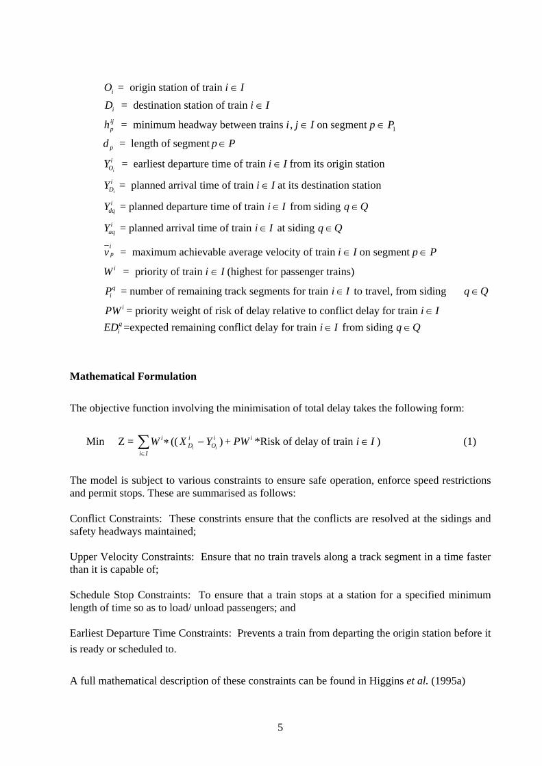
THE TRAIN SCHEDULING MODEL Definition of Variables The set of trains is given by I={1,2,.....,m,m+1,.....,N} for which inbound trains are from 1 to m and outbound are from m+1 to N. The ordering of the trains in this set considered in terms of expected departure time. The variables used in the paper are listed and described below. Let: P P P= { 1 2, } where: P P1 2= set of single line tracks, = set of double line tracks The arrival and departure time continuous decision variables are as follows: X i I q Qaq

i = arrival time of train at siding ∈ ∈

X i I q Qdqi = departure time of train from siding ∈ ∈

X i IOi

i = departure time of train from its origin station ∈

X i IDi

i = arrival time of train at its destination station ∈

The required input parameters for the model are defined as follows:

5

O i Ii = origin station of train ∈ D i Ii = destination station of train ∈

h i j I p Ppij = minimum headway between trains , on segment ∈ ∈ 1

d p Pp = length of segment ∈

Y i IOii = earliest departure time of train from its origin station∈

Y i IDi

i= planned arrival time of train at its destination station∈

Ydqi = planned departure time of train i I∈ from siding q Q∈

Yaqi = planned arrival time of train i I∈ at siding q Q∈

v i I p Ppi = maximum achievable average velocity of train on segment ∈ ∈

W i Ii = priority of train (highest for passenger trains)∈

Piq = number of remaining track segments for train i I∈ to travel, from siding q Q∈

PW i = priority weight of risk of delay relative to conflict delay for train i I∈ EDi

q =expected remaining conflict delay for train i I∈ from siding q Q∈ Mathematical Formulation The objective function involving the minimisation of total delay takes the following form: Min Z = W X Yi

Di

Oi

i Ii i

∗ −∈∑ (( ) + PW i *Risk of delay of train i I∈ ) (1)

The model is subject to various constraints to ensure safe operation, enforce speed restrictions and permit stops. These are summarised as follows: Conflict Constraints: These constrints ensure that the conflicts are resolved at the sidings and safety headways maintained; Upper Velocity Constraints: Ensure that no train travels along a track segment in a time faster than it is capable of; Schedule Stop Constraints: To ensure that a train stops at a station for a specified minimum length of time so as to load/ unload passengers; and Earliest Departure Time Constraints: Prevents a train from departing the origin station before it is ready or scheduled to. A full mathematical description of these constraints can be found in Higgins et al. (1995a)

6

CALCULATION OF RISK OF DELAY This section describes the train related risk of delay component of equation 1. The reader is referred to Higgins et al. (1995a) for the derivation of track and terminal related risk of delay. The following assumptions are made in conjunction with the train related risk of delay model: • A delaying train is a train that breaks down or slows down due to train dependent problems

and causes delay to other trains; • A siding/station will usually have enough room to accommodate only one train; • When a delaying train clears the track segment, all trains waiting which are to travel in the

same direction will be given right of way, since they can follow the delaying train on the same track segment. The conflict delay will be lower if all trains travelling in the same direction as the delaying train go first.

The following information is to be provided by the user: • The initial priority of each train. This may be a function of train type, (eg. passenger vs

freight train) and customer considerations; • The distribution of length of source delays and the probability of the delay occurring due to

unforeseen events on tracks and at sidings. A different set of distributions for each type of source delay must be obtained.

Figure 1 shows the regions which trains would be delayed due to a delaying train, where Tq is the length of time of source delay (unforeseen event).

7

q-1

q-1

q

q+1

q+1

q+2

Time

Point of Delay ec

a b d

q

Figure 1: Regions of delay for other trains when considering path of delaying train

Referring to Figure 1, if an inbound train (departing siding q-1∈Q and terminating at siding q+2∈Q) is to arrive at siding q+1∈Q at the time indicted by region a, it will experience a delay of at least the time indicated by b plus the time for the trains in the other direction to clear. If more than one train is to arrive at siding q+1∈Q in periods a and b, they will have to wait at sidings q+2, q+3∈Q and so on (if there are any outbound trains in region c), since the trains travelling in the same direction as the delaying train will clear first (in bulk). Region c represents the trains directly affected by the delaying train (travelling in the same direction). If a second outbound train has already departed siding q∈Q when the delaying train stops or slows down, it will wait on that track segment until the first train starts moving again. Region d represents inbound trains which are not directly affected by the delaying train, but are delayed by the clearing outbound trains. Region e is the set of trains travelling in the same direction as the delaying train which are affected by the clearing of trains (in bulk) from regions a and b. Region e will only apply if the trains travelling in the opposite direction to the delaying train clear first (ie. no trains in region c). If region e applies, the delaying train will wait at siding q+1∈Q for the other trains to cross. Region d will apply when region e does not. The determination of risk of delay due to track or terminal related unforeseen events are also based on the principles of these delay regions. Figure 1 refers to the case when an outbound train is the delaying train. The inbound delaying train instance is analogous. To construct the model, the following variables are defined using Figure 1 (for when the delaying train j I∈ is outbound).

Let Downset j q

Tq, be the set of trains travelling in the same direction as the delaying train j I∈

and arrive at siding q∈Q in the time marked by region c. Let NDS j qTq, be the number of trains in

Distanc

8

this set. Let Oppdownset j qTq, be the set of inbound trains that arrive at siding q+1∈Q in the

periods indicated by a and b, NODS j qTq, be the number of trains contained in this set (when

delaying train j I∈ is outbound). Let wj qTqRgiond , be the set containing any train(s) i I∈

travelling in the opposite direction to the delaying train, which pass through siding q+1∈Q in the period indicated by d, and conflicts with train j I∈ on track segment w P∈ 1 given its new

delayed path. These are the trains which are affected by the clearing of trains from region c after the delaying train has cleared. Let w

j qTqRgione , be the set containing any train(s) i I∈

travelling in the same direction as the delaying train, which passes through siding q∈Q in period e, and conflicts with train ch I∈ on track segment w P∈ 1 given its new delayed path.

The train ch I∈ is the first train travelling in periods a and b. A train i I∈ is classed as being in region a or b if: X X X X Tqaq

idqj

dqi

aqj> < ++ +, 1 1 and train j I∈ is outbound

X X X X Tqaqi

dqj

aqi

aqj

+ +> < +1 1 , and train j I∈ is inbound

A train i I∈ is classed as being in region c if: X X X Tq Xdq

idqj

dqi

dqj> < +, and train j I∈ is outbound

X X X Tq Xdqi

dqj

dqi

dqj

+ + + +> < +1 1 1 1, and train j I∈ is inbound

A train i I∈ is classed as being in region d if:

X X Tq X X Tq dvdq

iaqj

Oi

aqj k

kj

k Pi

cfq

+ + +∈

> + < + ++

∑1 1 11

, and train j I∈ is outbound

X X Tq X X Tq dvdq

iaqj

Oi

aqj k

kj

k Pi

cfq

> + < + +∈∑, and train j I∈ is inbound

This represents any train which crosses the path of the clearing of the trains travelling in the same direction as the delaying train. The path of the clearing of trains commences from when the trains travelling in the same direction as the delaying train begin to clear, until the termination station is reached. A train i I∈ is classed as being in region e if:

9

X X Tq X X Tq dvdq

idqj

Oi

aqj k

kch

k Pi

chq

> + < + ++∈ +∑, 1

1

and train j I∈ is outbound

X X Tq X X Tq dvdq

idqj

Oi

aqj k

kch

k Pi

chq

+ +∈

> + < + + ∑1 1 , and train j I∈ is inbound

The prioritised delay that would be suffered due to a delaying train suffering a source delay of Tq to clear to a siding, takes the form: priority*(delay due to delaying train - expected amount of time which can be recovered). The recoverability component is required to make an estimate of the delay at the destination. The actual recoverability of a train would not be known unless the schedule is resolved or optimised. This would have to be done for all combinations of source delay Tq. Since the time to do this would be prohibitive, an unbiased estimate of the recoverability is made. The analytical equation for the delay suffered by outbound train i I∈ due to another delaying outbound train j I∈ is:

W X Tq X X X Tq EDdv

iaqj

aqi

Di

aqj

iq k

ki

k Pi

iq

* (( ) ( ( ) ))+ + ++

∈

+ − − − + − −+

∑1 1 11

1

(2)

if i Downset j qTq∈ ,

and the delay to inbound train i I∈ due to outbound delaying train j I∈ is:

W X Tq NDS hdv

X X X

Tq NDS hdv

EDdv

iaqj

j qTq

pij

sNDS

zp s

p scf dq z

iDi

aqj

j qTq

pij

sNDS

zp s

p scf i

p z k

ki

k P

j qTq

i

j qTq

iq z

i

* ( * (

* ))

,

,

,

,

+=

≠

−+

++ +

=≠

−+

+

+

∈

+ + + − − − −

− − − −

∑

∑ ∑+

11

0

1

1

10

1 (3)

if i Oppdownset j qTq∈ ,

where:

zi Oppdownset NDS

NDSj qTq

qj

qj=≠=

⎧⎨⎪

⎩⎪

position of train in if if

, 01 0

The delay to outbound train i I∈ in region d, given an inbound delaying train j I∈ is:

10

W X Tq NDS h

dv

dv

X

X EDdv

iaqj

j qTq

pij s

scf

s q

ww s

w scf dw

i

s

z

Di

iw z k

ki

k Pi

iw z

* ( * * * * * *

( ))

,2 2 2 2 211

11

+ + + + −

− − −

+= −

−

−−

=

−

∈

∑ ∑

∑−

(4)

if i Rgiondwj qTq∈ +, 1

where:

zi Rgiond NODS q wj q

Tqj qTq

=− − +⎧

⎨⎩

+ +position of train in + if > otherwise

w, , ( )1 1 1 0

0

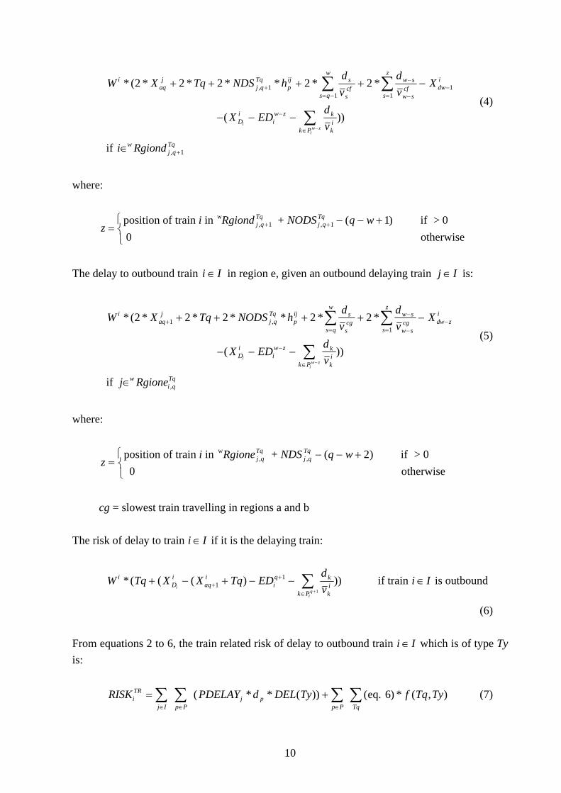
The delay to outbound train i I∈ in region e, given an outbound delaying train j I∈ is:

W X Tq NODS h

dv

dv

X

X EDdv

iaqj

j qTq

pij s

scg

s q

ww s

w scg dw z

i

s

z

Di

iw z k

ki

k Pi

iw z

*( * * * * * *

( ))

,2 2 2 2 211

+=

−

−−

=

−

∈

+ + + + −

− − −

∑ ∑

∑−

(5)

if j Rgionewi qTq∈ ,

where:

zi Rgione NDS q wj q

Tqj qTq

=− − +⎧

⎨⎩

position of train in + if > otherwise

w, , ( )2 0

0

cg = slowest train travelling in regions a and b

The risk of delay to train i I∈ if it is the delaying train:

W Tq X X Tq EDdv

iDi

aqi

iq k

ki

k Pi

iq

*( ( ( ) ))+ − + − −++

∈ +∑1

1

1

if train i I∈ is outbound

(6) From equations 2 to 6, the train related risk of delay to outbound train i I∈ which is of type Ty is: RISK PDELAY d DEL Ty f Tq Tyi

TR

j I p Pj p

p P Tq

= +∈ ∈ ∈∑ ∑ ∑ ∑( * * ( )) ( ) * ( , )eq. 6 (7)

11

1 2 4

5 6 7

Time

where: DEL Ty f Tq Ty

Tq w P

( ) (( ) ( ) ( ) ( )) * ( , )= + + +∑ ∑∈

eq. 2 eq. 3 eq. 4 eq. 5

PDELAYi = the probability of a train related delay occurring to delaying train i I∈

f(Tq,Ty) = the probability a train of type Ty will suffer a delay of length Tq. This is the source delay distribution.

The risk of delay to train i I∈ is RISKi

TR +Track related risk of delay+Terminal related risk of

delay. Calculation of Expected Remaining Conflict Delay

In this section, the expected remaining conflict delay EDiq is calculated for train i I∈ from

siding q Q∈ . The example considered in Figure 2 is when train 6 is inserted from siding 1. The

dashed line represents the unresolved path of train 6 which may be a new train inserted, or a delayed train at siding 1.

Figure 2: New path for train 6 for which EDiq must be calculated

When calculating ED6

1 for the delayed path of train 6, it is assumed the path of the other trains

are fixed up to the point of conflict with train 6. This is unlike the delay model proposed by Chen and Harker (1990) which calculates the expected conflict delay of each train in the schedule when the paths of all trains are variable.

1 1

2

2

3

3

4

4

5

3

Distanc

12

For the remainder of this section, train i I∈ is the delayed train for which the remaining conflict delay is to be calculated. The assumptions made with the conflict delay model are as follows: • The cumulative amount of conflict delay to the delayed train i I∈ between siding q Q∈

and the destination, is assumed to be normally distributed. The model is not restricted to the normality assumption, and other distributions which may better represent this delay can be used; and

• The path of any train other than the delayed train is assumed fixed. This is valid since the schedule is already resolved. The path of other trains do not change prior to the conflict with the delayed train. The arrival and departure time of train i I∈ at each siding q Q1∈

are X aqi

1 and X dqi

1 respectively. This is because the path of this train must be re-scheduled.

The arrival and departure times of each of the other trains j I∈ at each siding q Q1∈ are

Yaqj1 and Ydq

j1 respectively, since the path of these trains is already fixed.

Since the objective function involves the minimisation of delay, the probability that train i I∈

will be delayed by a train j I∈ in a conflict is WW W

j

i j+, as this is the proportion of time it is

more beneficial to delay train i I∈ . Let Gijp1 be the delay to train i I∈ due to train j I∈ on

track segment p P1 1∈ . From Petersen (1974), the expected delay is:

E( )( )

( )G

WW W d

vdvijp

j

i j p

pi

p

pj1

1

1

1

12= + ±

where the sign in the second term is '+' for a crossing and '-' for a overtake. Let SS pi

1 be the set

of trains j I∈ which have a probability of greater than zero of conflicting with train i I∈ , on track segment p P1∈ . The expected conflict delay to train i I∈ from all other trains on track

segment p P1∈ , is:

pp Gijp ijpj SS p

i1 1

1

* ( )E∈∑ (8)

where ppijp1 is the probability of train i I∈ conflicting with train j I∈ on track segment

p P1∈ , and is equal to:

P P( ) ( )X Y Xdv

Ydqi

aqj

dqi p

pi dq

j1 1 1

1

11 1< + > + i>m, j≤m

P P( ) ( )X Y Xdv

Ydqi

aqj

dqi p

pi dq

j1 1 1 1 1 1

1

11+ + +< + > j>m, i≤m

13

q+1

1 2

a

Distance

Time

P P( ) ( )X Y Xdv

Ydqi

dqj

dqi p

pi aq

j1 1 1

1

11 1< + > + i,j>m, i<j

P P( ) ( )X Y Xdv

Ydqj

dqi

dqj p

pi aq

i1 1 1

1

11 1< + > + i,j>m, i>j

P P( ) ( )X Y Xdv

Ydqi

dqj

dqi p

pi aq

j1 1 1 1 1 1

1

11+ + +< + > i,j≤m, i<j

P P( ) ( )X Y Xdv

Ydqj

dqi

dqj p

pi aq

i1 1 1 1 1 1

1

11+ + +< + > i,j≤m, i>j

Train i I∈ may meet with two trains on the same track segment and may be delayed by both (see Figure 3). The delay suffered to train i I∈ due to both trains is the maximum of these delays and not the addition, as would be calculated in equation 8.

Figure 3: Conflict with two trains on same segment Given that train j I∈ is the first train and j I+ ∈1 is the second train, the expected amount of delay subtracted from equation 8 is:

P(train i I∈ conflicts with trains j j I and + ∈1 on segment p P1 1∈ )*P(train i I∈ is

delayed by train j+1∈I on segment p P1 1∈ )*E( Gijp1 ) = Qijp1 *E( Gijp1 )

where: P(train i I∈ conflicts with trains j j I and + ∈1 on segment p P1 1∈ ) =

P P( ) ( )X Y Xdv

Ydqi

aqj

dqi p

pi dq

j1 1 1

1

11 11< + > ++ i >m, j,j+1≤m (9)

P P( ) ( )X Y Xdv

Ydqi

aqj

dqi p

pi dq

j1 1 1 1 1 1

1

111

+ + ++< + > i≤ m, j,j+1>m (10)

p

q 3

b

14

If train i I∈ is outbound, the expected delay to train i I∈ before and including track segment p P1 1∈ is:

E pi

1 = E pi1 1− + pp Gijp ijp

j SS pi

1 11

* ( )E∈∑ - Q Gijp ijp1 1* ( )E i>m (11)

If train i I∈ is inbound, the expected delay to train i I∈ after and including track segment p P1 1∈ is:

E pi1

# = E pi1 1+

# + pp Gijp ijpj SS p

i1 1

1

* ( )E∈∑ - Q Gijp ijp1 1* ( )E i≤m (12)

The calculation of the variance is similar to that of Chen and Harker (1990) and is given by: Vp

i1 = Vp

i1 1− + ( ) * ( ) ( )( ) * ( ( ))pp Q G pp Q pp Q Gijp ijp ijp ijp ijp

j SSijp ijp ijp

pi

1 1 1 1 1 1 121

1

− + − − +∈∑ V E +

COV( , )k SSj SS

ijp ikppi

pi

o o∈∈∑∑

11

1 1 i>m, j,k≤m (13)

V pi1

# = V pi1 1+

# + ( ) * ( ) ( )( ) * ( ( ))pp Q G pp Q pp Q Gijp ijp ijp ijp ijpj SS

ijp ijp ijppi

1 1 1 1 1 1 1 121

1

− + − − +∈∑ V E +

COV( , )k SSj SS

ijp ikppi

pi

o o∈∈∑∑

11

1 1 i≤m, j,k>m (14)

where:

V( ) ( ) * ( ) ( )Gd W

W Wdv

dvijp

p j

i j

p

pi

p

pj1

1 2 1

1

1

1

2

314

= −+

+

oijp1 = Gijp1 when train i I∈ conflicts with train j I∈ on segment p P1 1∈ , and train i I∈ is

not delayed by train j I+ ∈1 on segment p P1 1∈

oijp1 =0 otherwise

COV( , )o oijp ikp1 1 =P(train i I∈ conflicts with trains j k I, ∈ on segment p P1 1∈ and train

i I∈ is not delayed by trains j k I+ + ∈1 1, on segment p P1 1∈ )* E( , )G Gijp ikp1 1 - ( ) * ( ) * ( ) * ( )pp Q pp Q G Gijp ijp ikp ikp ijp ikp1 1 1 1 1 1− − E E

P(train i I∈ conflicts with trains j k I, ∈ on segment p P1 1∈ and train i I∈ is not delayed

by trains j k I+ + ∈1 1, on segment p P1 1∈ )

= P(train i I∈ conflicts with trains j k I, ∈ ) - P(train i I∈ conflicts with trains j,k, j k I+ + ∈1 1, and is delayed by trains j k I+ + ∈1 1, on segment p P1 1∈ )

P(train i I∈ conflicts with trains j,k, j k I+ + ∈1 1, and is delayed by trains j k I+ + ∈1 1, on segment p P1 1∈ ) =

P P( ) ( )X Y Xdv

Ydqi

aq dqi p

pi dq1 1 11

11 1

1< + > ++α β * ppi pβ 1 i>m

15

P P( ) ( )X Y Xdv

Ydqi

aq dqi p

pi dq1 1 1 1 1 1

1

11

1+ + +

+< + >α β * ppi pβ 1 i≤ m

α =min(j,k), β =max(j,k).

It is assumed the covariance between Vpi1 1− and the second term in equation 13 is zero. The

same applies to V pi1 1+

# in equation 14. It is assumed that X dqi

1 is normally distributed with mean

Ydqi

1 + DT + E pi

1 and variance Vpi1 if i>m, and with mean Ydq

i1 + DT + E p

i1 1−

# and variance V pi1 1−

# if

i≤ m. The model is not confined to the arrival and departure times being normally distributed. In practical situations, it is more likely the arrival/departure times will be a skewed distribution with the tail towards late arrivals/departure times. Solving equations 12 and 14 requires the solution to a system through an iterative method. There are NS-1 systems of equations to solve, where NS is the number of sidings. An efficient method is as follows: Let t

piE 1 , t

piE 1

# , tpiV 1 , t

piV 1

# have the same definition as E pi

1 , E pi1

# ,Vpi1 ,V p

i1

# except at iteration t. Let:

X dq

i1∼N(Ydq

i1 + DT + t

piE 1 1− , t

piV 1 1− ) t=1,i>m

X dqi

1∼N(Ydqi

1 + DT + tpiE−1

1 , tpiV−11 ) t>1,i>m

X dqi

1∼N(Ydqi

1 + DT + tpiE 1 , t

piV 1 ) t=1,i≤m

X dqi

1∼N(Ydqi

1 + DT + tpiE−−

11 1 , t

piV−−

11 1 ) t>1,i≤m.

The algorithm to determine t

piE 1 , t

piE 1

# , tpiV 1 , t

piV 1

# , and EDiq is:

0. Let t=0. 1. Let t=t+1, t

piE −1 = t

piE # = t

piV −1 = t

piV # =0.0 assuming no unforeseen events.

IF i>m, obtain tpiE 1 and t

piV 1 for all segments p P1 1∈ s.t. p1>p-1 and p1< Di .

IF i≤m, obtain tp

iE 1# and t

piV 1

# for all segments p P1 1∈ s.t. p1<p and p1≥ Di .

2. IF i>m and tpi t

piE E1

11 1− <− ε , t

pi t

piV V1

11 2− <− ε (where ε ε1 2, are small) ∀ ∈p P1 1 s.t. p1>p-

1 and p1< Di , THEN

Go to Step 3.

ELSE IF i≤m and tpi t

piE E1

11 1

# #− <− ε , tp

i tp

iV V11

1 2# #− <− ε ∀ ∈p P1 1 s.t. p1<p and p1≥ Di ,

THEN Go to Step 3. ELSE

16

Go to Step 1. END {IF}. 3. IF i>m THEN EDi

q = tDiE

i −1

ELSE EDi

q = tD

iEi

# .

END {IF}.

SOLUTION TECHNIQUES The single line train scheduling model is solved using optimal and heuristic solution techniques. Since the problem is NP-Hard, larger problem sizes may only be able to be solved in real-time using heuristic techniques. Optimal Solutions The best known technique for optimising the train scheduling problem is by branch and bound. A depth first search is used for the resolution of conflicts. Each node in the branch and bound tree represents a partial solution (ie. partially resolved schedule), and the depth (in terms of number of levels) in the tree determines the number of conflicts resolved in this partial solution. A node at the ninth level of the tree will be a partially resolved schedule where the first nine conflicts are resolved. Each node will have two branches as either of the two trains in the conflict can be delayed. A train is delayed at the nearest feasible siding. The arrival and departure times of the trains in each partial solution are determined by solving the linear/non-linear sub-problem (integer variables fixed). Full details of the branch and bound technique as well as the lower bound can be found in Higgins et al. (1996) Heuristic Solution Techniques Although improved lower bounds for the branch and bound procedure reduce the calculation time, the optimal solution cannot be guaranteed in any less time. Test results show that the problems solved are all optimised within a fixed time (say X minutes) but this is not a guarantee that all possible problems of this size will be solved within X minutes. This would be a problem if the branch and bound technique was used to schedule trains in real-time.

17

Nearest Neighbourhood Heuristic The nearest neighbourhood heuristic (NNH) is the most common of such heuristics. Before it can be applied, a feasible initial solution must be obtained. The initial solution can be obtained by several methods, such as early terminated branch and bound procedure, simulation or another heuristic which does not start with an initial solution. The heuristic works by taking a conflict (keeping all other conflicts fixed) and resolving it on each neighbouring siding. If the solution is improved it is kept, otherwise the old solution remains. Feasibility must be ensured at all times when testing for improvement as a move may cause two trains to be at a siding at once. The main disadvantage of the general NNH is that a move only shifts the position of one conflict at a time. Situations do occur where shifting the position of two or more conflicts at the same time is the only way to improve the solution. The complexity order grows when considering a move which shifts the position of more than one conflict simultaneously. The size of the neighbourhood for which a move shifts one conflict is of order O( CO ) where CO is the number of conflicts in the schedule. When testing a move involving a simultaneous shift of n conflicts, the number of moves to be tested is up to 2n CO

nC* . Implementation on a computer would be prohibitive for anything other than the smallest of problems. Due to the way trains interact, not all of these moves need to be tested. For a move which shifts the position of two conflicts, only two neighbouring conflicts (where one train is involved in both) need to be considered, as the outcome of shifting one conflict is not directly related to the outcome of shifting the other, when they are not neighbouring. Also, two directly dependent conflicts will have a train in common and if one of the conflicts is shifted further outbound so will the other. This reduces the size of the neighbourhood to be linear with respect to the number of conflicts. The new neighbourhood is defined as follows: When considering a particular conflict in a train schedule, there are four possible moves. For the outbound train, all of the remaining conflicts for that train can be moved one siding inbound from the current position, or one siding outbound from the current position. The same applies to the inbound train in the conflict. Genetic Algorithms (GA) Since the train scheduling problem is a linear/non-linear mixed integer program, whenever a new solution is produced, its fitness must be evaluated by solving a linear/non-linear program. For GA (Goldberg, 1989; Davis, 1987 and 1991; and Spears et al., 1991), an efficient string representation must be established that will allow a smaller population to be used and faster convergence without sacrificing solution quality.

18

2

1 3

4 5 6

Distance

Time

The best representation is to use each conflict in the train schedule instance as a gene. Each gene will contain the delayed train, the train with right of way and the track segment which the conflict occurs. This is illustrated in Figure 4. The first conflict is between trains 1 and 4 on track segment 2. Train 1 is delayed and thus takes the first place in the gene.

1,4,2 2,4,3 5,1,2 5,2,3 3,5,3 6,3,2Parent

Gene 1 Gene 2 Gene 3 Gene 4 Gene 5 Gene 6

Figure 4a: Chromosome representation of train schedule (shown in Figure 1b)

Figure 4b: Six conflict train schedule

Just changing one conflict (gene) is found not to be a good form of mutation in the train scheduling problem. A mutation here is the selection of a move from the new neighbourhood as there is a greater probability of improving the solution. The travel time of each train on each track segment is used to filter out moves which are more likely to improve the solution. It is desirable to keep the initial population as small as possible so as to keep the number of generations small. The population is generated using a probabilistic method. Each resolved train schedule instance is generated by resolving each of the conflicts as they appear in time at one of the two nearest sidings. The probability of resolving the conflict at the siding is a function of the conflict delay that would occur. Tabu Search (TS) TS (Glover 1990 and 1993) is applied to the train scheduling problem in the same way as the NNH. The base version is defined as follows: A move will shift one conflict. A sample of the neighbourhood is taken randomly where moves drawn probabilistically in terms of the

2

3 3

4 4

5 2

1 1

19

likelihood of improving the solution. Although this creates a biased sample of the neighbourhood, good moves are found more often. Moves which create infeasible solutions are discarded. If new unresolved conflicts are found after a move, they are resolved by moving the conflict to the nearest feasible siding. Different modifications were made to the base version and were tested on train schedules for which the size varied between 12 and 110 conflicts or between 9 and 50 trains. The approaches which improved on the base version are summarised below. Improved Neighbourhood: Uses the improved neighbourhood structure instead of only shifting a single conflict in each move. The new neighbourhood worked well on most problems but poorly on some. This is because the new neighbourhood could not allow some single conflict moves to be performed. Intensified Search: Temporarily searches a larger portion of the neighbourhood when a new best solution so far is found. The method requires more calculations but gives all round improvement over the base version. Penalty Search: Penalises a move by adding to the objective function a constant multiplied by the number of times the move had been tried previously. This method was found to prevent long term repetition and worked well on most problems. New Initial Solution: When diversification is performed, a new initial solution is generated randomly using the same method as for genetic algorithms. This appears to be a good form of diversification for the train scheduling problem, since the new initial solution may be totally different from the previous one. This version along with the intensified search version produced the best results overall. Comparisons of Solution Techniques Comparisons were made between each of the heuristics and the optimal solution when using the branch and bound technique. The results, in terms of average increase in conflict delay over the optimal solution, are shown in Table 1. The GA and TS techniques produced better results than the NNH on all problems, with the GA results out-performing the TS on most occasions. The NNH with the new neighbourhood gave better results than the neighbourhood which moves one conflict at a time. This was more evident for larger problems. The TS and GA heuristics required significantly more calculations than the NNH. The number of calculations did not increase significantly with problem size for any heuristic (as was the case with a branch and bound procedure).

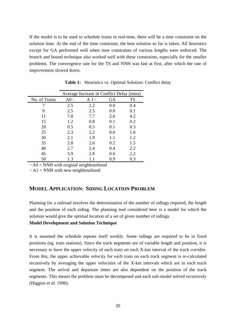
20

If the model is to be used to schedule trains in real-time, there will be a time constraint on the solution time. At the end of the time constraint, the best solution so far is taken. All heuristics except for GA performed well when time constraints of various lengths were enforced. The branch and bound technique also worked well with these constraints, especially for the smaller problems. The convergence rate for the TS and NNH was fast at first, after which the rate of improvement slowed down.

Table 1: Heuristics vs. Optimal Solution: Conflict delay

Average Increase in Conflict Delay (mins) No. of Trains A0 ( )1 A 1 ( )2 GA TS

7 2.5 2.2 0.0 0.4 9 2.5 2.5 0.0 0.1 11 7.8 7.7 2.6 4.2 15 1.2 0.8 0.1 0.2 20 0.5 0.5 0.1 0.3 25 2.3 2.2 0.0 1.6 30 2.1 1.9 1.1 1.2 35 2.8 2.6 0.2 1.5 40 2.7 2.4 0.4 2.2 45 5.9 2.8 0.6 2.2 50 1.3 1.1 0.9 0.3

( )1 A0 = NNH with original neighbourhood ( )2 A1 = NNH with new neighbourhood

MODEL APPLICATION: SIDING LOCATION PROBLEM Planning for a railroad involves the determination of the number of sidings required, the length and the position of each siding. The planning tool considered here is a model for which the solution would give the optimal location of a set of given number of sidings. Model Development and Solution Technique It is assumed the schedule repeats itself weekly. Some sidings are required to be in fixed positions (eg. train stations). Since the track segments are of variable length and position, it is necessary to have the upper velocity of each train on each X-km interval of the track corridor. From this, the upper achievable velocity for each train on each track segment is re-calculated recursively by averaging the upper velocities of the X-km intervals which are in each track segment. The arrival and departure times are also dependent on the position of the track segments. This means the problem must be decomposed and each sub-model solved recursively (Higgins et al. 1996).

21

An initial unresolved schedule and initial siding positions will be input to the solution procedure. If no initial sidings positions are available, they can be estimated using simulation or by assuming the sidings to be equally spaced. The first sub-model determines the optimum train schedule and is solved using the branch and bound technique. The second sub-model is a constrained non-linear program and can be solved using a specialised software package such as GAMS/MINOS 5.2 (Brooke et al. 1988). The purpose is the determination of the optimum siding positions given a fixed train schedule. The decision variables are now the track segment lengths and the arrival and departure times of the trains. Output from the second sub-model is used as input to the first. If the conflict resolution strategy does not change from one iteration to the next, the sidings are at the improved locations and the algorithm has converged. Output from the algorithm is the improved siding locations with the associated optimal train schedule. Model Testing The model was tested on a problem consisting of 20 scheduled trains and 8 sidings. The problem was chosen to demonstrate the advantage of having the sidings at the optimal locations. The objective of the model was to delay due to conflicts as well as risk of delay. The first sub-problem in Figure 4 was solved using the branch and bound technique and the second sub-problem was solved using GAMS/MINOS. The decomposition procedure converged in 3 iterations and within 4 minutes on a 80486DX PC. The optimal schedules given the current and improved siding positions are demonstrated in Figures 4a and 4b respectively. The total conflict delay for this schedule is 0.9 hours less, and the total delay (conflict delay plus risk of delay) is 0.4 hours less, than when the sidings are positioned with respect to conflict delay only.

Figure 4a: Optimal schedule given current siding locations

22

Figure 4b: Optimal schedule given improved siding locations

CONCLUSIONS This paper has briefly described two inter-related models: one which optimises a given pattern of train demand operating mainly under single track conditions; and another which estimates the likely risk of trains being delayed. The results of the latter model are then used to optimise schedules taking into account train trip times, as well as reliability of arrival times. Although the models presented here are aimed mainly at train operations over single track, the basic principles can be applied to multi-track operations, by modifying the reliability estimation procedure and the conflict resolution algorithms. The models can be used to provide an aid to train dispatchers in resolving train conflicts under single track operations; and they can also be used to plan the introduction of new services, by allowing estimates to be made of the likely resultant changes in reliability of train arrivals over the entire timetable. The likely impact of track, train and station/terminal investment, on train trip times and arrival reliability can be estimated by optimising a given schedule with and without the investment under study. The risk of delay component of the objective function was separated into three categories, namely: train, track and terminal related delay. For each delay category, the calculation of risk of delay was based on modelling the effects on trains due to a probability distribution of unforeseen events. When an unforeseen event occurs, a train can be directly or indirectly affected. Both situations were modelled for all three delay categories. The risk of delay to a train given an unforeseen event was calculated as the length of delay due to the unforeseen event minus the amount of time which can be recovered. Optimal and heuristic solution techniques were used to solve a constrained optimisation model. The optimal solution technique is branch and bound based, and uses improved lower bound estimates of the remaining conflict delay to reduce the search space in the branch and bound tree. Three heuristics applied to the train scheduling problem. For the nearest neighbourhood

23

heuristic, an improved neighbourhood structure which allows the position of more than one conflict to be changed in a single move was presented. Genetic algorithms and tabu search were also applied to the train scheduling problem. An efficient problem representation was used for the genetic algorithm which allows the use of small population sizes. Several different versions of the tabu search heuristic were tested, with most versions differing in terms of how intensification/ diversification was performed. The genetic algorithm performed best out of all heuristic techniques when allowed to fully converge. When time constraints are enforced (as in the case in practice), the tabu search achieved the best results all round. The genetic algorithm performed poorly compared to the other heuristic and optimal solution techniques. The optimisation techniques were used to assist in determining the best position of sidings on a track corridor. A decomposition procedure was used iteratively to solve for the best siding positions, and best resolved schedule simultaneously. The branch and bound technique optimised the train scheduling sub-problem, and a specialised software package was used to solve the optimal siding location (fixed schedule) sub-problem. The siding location model can be used to determine the optimum number of sidings, as well as to position these sidings.

REFERENCES Brooke, A., Kendrick, D. and Meeraus, A. (1988). “GAMS: A User's Guide”, Scientific Press. Cai, X. and Goh, C. J. (1992). “A Fast Heuristic for the Train Scheduling Problem”, Optimisation: Techniques and Applications, 1, 596 - 603. Carey, M. and Kwiecinski, A. (1994). “Stochastic Approximation to the Effects of Headways on Knock-on Delays of Trains”, Transportation Research B, 28, 251-267. Chen, B. and Harker, P. (1990). "Two Moments Estimation of Delay on Single-Track Rail Lines with Scheduled Traffic", Transportation Science, 24, 261 - 275. Davis, L. (1987). Genetic Algorithms and Simulated Annealing, Pitman. Davis, L. (1991). Handbook on Genetic Algorithms, New York: Van Nos-trand Reinhold. Glover, F. (1990). "Tabu Search: A Tutorial", Interfaces, 20, 74 - 79. Glover, F. (1993). "A Users Guide to Tabu Search", Annals of Operations Research, 41, 3 - 28.

24

Goldberg, D. E. (1989). Genetic Algorithms in Search, Optimisation, and Machine Learning, Addison-Wesley. Hallowell S. (1993). “Optimal Dispatching Under Uncertainty: with Applications to Railroad Scheduling”, PhD Thesis, Department of Decision Sciences, Wharton School, University of Pennsylvania. Harker, P. and Hong, S. (1990). “Two Moments Estimation of the Delay on a Partially Double-Track Rail Line with Scheduled Traffic”, Transportation Research Forum, 30, 38 - 49. Higgins, A., Ferreira, L. and Kozan. (1996). “Modelling Single Line Rail Operations”, Transportation Research Record, 1489. Higgins, A., Kozan, E. and Ferreira, L. (1996). "Optimal Scheduling of Trains on a Single Line Track", Transportation Research B, 30, 147-161. Higgins, A., Ferreira, L and Kozan, E. (1995a). "Modelling Delay Risks Associated with Train Schedules", Transportation Planning and Technology, 19, 89 - 108. Higgins, A., Kozan, E and Ferreira, L. (1995b). "Rescheduling of Trains on a Single Line Track: Improved Heuristic Solution Techniques", Physical Infrastructure Research Report , 1-95, Queensland University of Technology, Brisbane. Jovanovic, D. (1989). "Improving Railroad On-time Performance: Models, Algorithms and Applications", PhD Thesis, Department of Decision Sciences, The Wharton School, University of Pennsylvania. Kraft, E. R. (1987). "A Branch and Bound Procedure for Optimal Train Dispatching", Journal of the Transportation Research Forum, 28, 263 - 276. Kraay, D. (1993). "Learning Methods in Optimisation: With Applications to Railroad Control", PhD Thesis at the Department of Decision Sciences. The Wharton School. University of Pennsylvania. Kraay, D., Harker, P. and Chen, B. (1988). "Optimal Pacing of Trains in Freight Railroads: Model Formulation and Solution", Working Paper 88-03-03, Decision Sciences Department, The Wharton School, University of Pennsylvania.

25

Kraay, D., Harker, P. and Chen, B. (1991). "Optimal Pacing of Trains in Freight Railroads", Operations Research, 39, 82 - 99. Mills, R. G., Perkins, S. E. and Pudney, P. J. (1991). "Dynamic Rescheduling of Long Haul Trains for Improved Timekeeping and Energy", Asia-Pacific Journal Operational Research, 8, 146 - 165. Petersen, E. R. (1974). "Over the Road Transit Time for a Single Track Railway", Transportation Science, 8, 65 - 74. Spears, W. M., Dejong, K. A., (1991). "An analysis of multi-point crossover" Foundations of Genetic Algorithms, G. J. E. Rawlins Ed, 301 - 315. Szpigel, B. (1973). "Optimal Train Scheduling on a Single Line Railway", Operations Research 72, 344 - 351.