1998 development of an atmospheric pressure microwave
TRANSCRIPT

University of WollongongResearch Online
University of Wollongong Thesis Collection University of Wollongong Thesis Collections
1998
Development of an atmospheric pressuremicrowave induced plasma beamStephen Allan GowerUniversity of Wollongong
Research Online is the open access institutional repository for theUniversity of Wollongong. For further information contact ManagerRepository Services: [email protected].
Recommended CitationGower, Stephen Allan, Development of an atmospheric pressure microwave induced plasma beam, Doctor of Philosophy thesis,School of Electrical, Computer and Telecommunications Engineering, University of Wollongong, 1998. http://ro.uow.edu.au/theses/1946


DEVELOPMENT OF AN ATMOSPHERIC PRESSURE MICROWAVE INDUCED PLASMA BEAM
A thesis submitted in fulfilment of the
requirements for the award of the degree
DOCTOR OF PHILOSOPHY
from
THE UNIVERSITY OF WOLLONGONG
by
STEPHEN ALLAN GOWER, BSC (HONS)
SCHOOL OF ELECTRICAL, COMPUTER AND
TELECOMMUNICATIONS ENGINEERING
1998

TABLE OF CONTENTS.
ABSTRACT I
LIST OF PUBLICATIONS/CONFERENCE PROCEEDINGS HI
LIST OF FIGURES VII
LIST OF TABLES XVII
ACKNOWLEDGEMENTS XVHI
CHAPTER 1. LITERATURE REVIEW 1
1.1 INTRODUCTION 1
1.2 REVIEW OF MICROWAVE CAVITY THEORY 1
1.3 A CHRONOLOGY OF APPLICATOR DEVELOPMENT 8
1.4 DETERMINATION OF PLASMA PARAMETERS 42
1.5 SUMMARY OF LITERATURE REVIEW.... 54
1.6 CONCLUSION 57
CHAPTER 2. EXPERIMENTAL DESIGN, EQUIPMENT AND PROCEDURES 61
2.1 INTRODUCTION 61
2.2 PULSED POWER SUPPLY 62
2.3 CONTINUOUS WAVE POWER SUPPLY 63
2.4 CIRCULATOR 64
2.5 DUAL DIRECTIONAL COUPLER 65
2.6 THREE STUB TUNER 66
2.7 SLOTTED WAVEGUIDE SECTION 67
2.8 POWER METER 68
2.9 MICROWAVE LEAKAGE METER 68
2.10 WELDING TABLE AND CONTROLLER 68
2.11 EXPERIMENTAL PROCEDURE 69
2.12 CONCLUSION 70
ii
CHAPTER 3. APPLICATOR DEVELOPMENT 71
3.1 INTRODUCTION 71
3.2 CYLINDRICAL CAVITY DESIGN 71
3.3 RECTANGULAR CAVITY DESIGN 82
3.4 WAVEGUIDE CAVITY DESIGN 84
3.5 WATER-COOLED WAVEGUIDE CAVITY DESIGN 88
3.6 CONCLUSION 96
CHAPTER 4. CHARACTERISATION OF THE PLASMA/APPLICATOR SYSTEM 99
4.1 INTRODUCTION 99
4.2 BACKGROUND THEORY OF VSWR 101
4.3 VSWR MEASUREMENTS ON THE NON-COOLED WAVEGUIDE APPLICATOR 102
4.4 ELECTRIC CIRCUIT MODEL OF THE WAVEGUIDE APPLICATOR 117
4.5 PLASMA IMPEDANCE MEASUREMENTS 124
4.6 VSWR MEASUREMENTS ON THE WATER-COOLED WAVEGUIDE APPLICATOR 129
4.7 PLASMA IMPEDANCE MEASUREMENTS ON THE WATER-COOLED WAVEGUIDE APPLICATOR. 131
4.8 PLASMA IMPEDANCE COMPARISONS 142
4.9 PLASMA BEAM LENGTH 143
4.10 HEAT CAPACITY OF THE PLASMA BEAM 153
4.11 PLASMA BEAM PRESSURE 158
4.12 CONCLUSION 161
CHAPTER 5. PLASMA TEMPERATURE DETERMINATION BY LASER SCATTERING
TECHNIQUES 165
5.1 INTRODUCTION 165
5.2 TEMPERATURE DETERMINATION 166
5.3 TEMPERATURE COMPARISONS 191
5.4 CONCLUSION 194

CHAPTER 6. APPLICATION OF THE PLASMA BEAM TO WELDING OF SHEET STEEL .
197
6.1 INTRODUCTION 197
6.2 RESULTS OF WELDING TRIALS 198
6.3 MODELLING OF WELDING PARAMETERS 209
6.4 COMPARISON WITH CONVENTIONAL WELDING TECHNIQUES 213
6.5 CONCLUSION 218
CHAPTER 7. CONCLUSION 219
CHAPTER 8. SUGGESTIONS FOR FURTHER WORK 230
8.1 INTRODUCTION 230
8.2 THE USE OF DIFFERENT DISCHARGE GASES 230
8.3 INCREASING THE ENERGY DENSITY AT THE WELD POOL 230
8.4 BEAM SHAPING TECHNIQUES 231
8.5 APPLICATION TO WELDING STEEL 231
8.6 APPLICATION TO WELDING CERAMICS 232
8.7 APPLICATION TO WELDING OF PLASTICS 232
8.8 APPLICATION TO CHEMICAL VAPOUR DEPOSITION OF DIAMOND FILMS 233
8.9 APPLICATION TO PLASMA SPRAYING 233
REFERENCES 234
APPENDKA 239
ENGINEERING DRAWING OF THE THREE-STUB TUNER GENERAL ASSEMBLY 239
APPENDIX B 240
ENGINEERING DRAWINGS OF THE PLASMA BEAM APPLICATOR AND COMPONENTS 240
REFERENCES 234
IV

ABSTRACT
Development of a device capable of producing a high power atmospheric pressure
plasma beam has been one of the goals of researchers since the development of the
magnetron. Until now, progress has been hampered for a variety of technical reasons
not the least being materials limitations and the unavailability of suitable microwave
generators. The work set forth in this dissertation describes the development of an
efficient, atmospheric pressure, plasma beam applicator capable of sustained operation
at powers in excess of 5 kW. Sustained operation at such high powers is accomplished
through innovative cooling techniques. The operating parameters necessary to produce
a stable plasma beam are elaborated upon, as are the physical properties of the plasma.
Properties such as beam temperature, length and pressure are characterised as a function
of the operating parameters of the system. Beam temperatures are determined using
laser scattering techniques from which 2D temperature profiles of the beam are
reconstructed.
The voltage standing wave ratio and complex impedance of the plasma are determined
as a function of microwave power, discharge gas flow rate and state of tuning of the
applicator for both cooled and non-cooled versions of the waveguide applicator. An
electric circuit model of the plasma/applicator system is then derived from these
measurements. Temperatures and impedances are compared to those reported in the
literature for similarly generated microwave plasmas.
Application of a microwave plasma beam to welding and joining applications is totally
absent from the literature. In this thesis, autogenous butt welding of sheet steel is
I

detailed and examination of the weld strength and weld microstructure as a function of
microwave power, discharge gas flow rate and travel speed performed. Results indicate
that welds performed using a microwave plasma beam are comparable in appearance
and quality to those generated using gas tungsten arc welding techniques.
n

LIST OF PUBLICATIONS/CONFERENCE PROCEEDINGS
Title: Microwave Induced Plasma Jet Welding and Joining.
Authors: S. A. Gower and D. DoRego.
Venue: CRC Project Number 93/15 Annual Technical Progress report, 1994.
Title/Seminar: Modelling of a Microwave Plasma Jet.
Authors: S. A. Gower and F. J. Paoloni
Venue: 20th AESfSE Plasma Physics Conference, Flinders University, 13th - 14th
of February, 1995.
Seminar:
Authors:
Venue:
A Microwave Induced Plasma Jet Welder (MIPJ).
S. A. Gower.
th cth C R C Project Leaders Meeting, CSIRO D M T Adelaide, AT - 5 m of April,
1995.
Seminar:
Authors:
Venue:
Modelling of a Microwave Plasma Jet.
S. A. Gower and F. J. Paoloni.
Inaugural JWRI-CRC for Material Welding and Joining Technical
:th Exchange, 6m of April, 1995.
Seminar: A Microwave Induced Plasma Jet Welder (MIPJ}
Authors: S. A. Gower.
Venue: W T I A Ulawarra Branch, Monthly Meeting, 21st of June, 1995.
ffl
Poster/Seminar: Microwave Induced Plasma Jet Welding (MIPJ).
Authors: S. A. Gower.
Venue: Postgraduate Research Student Open Day, 31 of August, 1995
Seminar: Applications of a Microwave Induced Plasma Jet.
Authors: S. A. Gower.
Venue: Vacuum arc ion beam workshop, Lawrence Berkeley National Labs,
Berkeley California, 25th - 28th of September, 1995.
Title: Microwave Induced Plasma Jet (MIPJ) Welding and Joining.
Authors: S. A. Gower.
Venue: 1994-1995 CRC for Materials Welding and Joining Annual Report.
Seminar: Microwave Induced Plasma Jet Welding and Joining.
Authors: S. A. Gower.
Venue: 2nd JWRI-CRC Technical Exchange, University of Wollongong, 11th of
March, 1996.
Seminar: Microwave Induced Plasma Jet.
Authors: S. A. Gower.
Venue: W T I A Panel 14 meeting, CSIRO Lindfield, Sydney, April 1996.

Title:
Venue:
High Power Microwave Gas Plasma Generation.
Authors: S. A. Gower, D. McLean and F. J. Paoloni.
th Australian Provisional Patent #PO0286, 6m of June, 1996
Seminar: Microwave Induced Atmospheric Pressure Plasma Jet.
Authors: S. A. Gower, C. Montross and F. J. Paoloni.
Venue: 12th Australian Institute of Physics Congress, University of Hobart, 1
5th of July, 1996.
St
Title/Seminar: Microwave Induced Plasma Jet for Welding.
Authors: S. A. Gower, D. DoRego and D. McLean.
Venue: Scientific and Industrial RF and Microwave Applications Conference,
RMIT, 9th-10th of July, 1996.
Seminar: Microwave Induced Plasma Jet Welding.
Authors: S. A. Gower.
Venue: th Industrial Automation Research Centre Meeting, 5 of September, 1996
Poster: Microwave Induced Plasma Jet Welding.
Authors: S. A. Gower and D. DoRego.
Venue: Post Graduate Research Student Open Day, 17th of September, 1996.
V

Title: Microwave Induced Plasma Jet Welding of Sheet Steel.
Authors: S. A. Gower, D. DoRego and A. Basu.
Venue: Australasian Welding Journal-Research Supplement, Vol 42, 40-46,
1997.
VI

LIST OF FIGURES.
FIGURE 1. EVOLUTION OF A CAVITY RESONATOR FROM A SIMPLE LC CIRCUIT, [l] 2
FIGURE2. COORDINATE SYSTEM AND DIMENSIONS USED FORTE MODE FIELD DERFVATION [3] 3
FIGURE 3. ELECTRIC AND MAGNETIC FIELD LINES FOR A TE101 RECTANGULAR CAVITY [3] 6
FIGURE4. SECTIONS THROUGH A CYLINDRICAL CAVITY SHOWING TM010 FIELD PATTERNS [3] 7
FIGURE 5. THE "ELECTRONIC TORCH" OF COBINE AND WILBUR [4], 1951 9
FIGURE6. THE TAPERED WAVEGUIDE APPLICATOR OF FEHSENFELD [5], 1965 11
FIGURE7. THE FORESHORTENED 3/4 WAVE COAXIAL APPLICATOR OF FEHSENFELD [5], 1965 12
FIGURE 8. THE FORESHORTENED 3/4 COAXIAL APPLICATOR OF FEHSENFELD [5], 1965 12
FIGURE 9. THE FORESHORTENED 1/4 WAVE RADIAL APPLICATOR OF FEHSENFELD [5], 1965 13
FIGURE 10. THE COAXIAL TERMINATION APPLICATOR OF FEHSENFELD [5], 1965 13
FIGUREII. THE FORESHORTENED 1/4 WAVE COAXIAL APPLICATOR OF FEHSENFELD [5], 1965 14
FIGURE 12. SCHEMATIC LAYOUT OF A COAXIAL PLASMA TORCH AS DESCRIBED BY SWIFT [12], 1966 15
FIGURE 13. WAVEGUIDE CONFIGURATION OF THE DISCHARGE GENERATOR OF MURAYAMA[ 13], 1968. 16
FIGURE 14. SCHEMATIC LAYOUT OF THE "MICROWAVE PLASMATRON" AS DESCRIBED BY ARATA ET AL
[14], 1973 17
FIGURE 15. CROSS SECTIONAL FRONT VIEW OF THE 30 KW PLASMATRON AS DESCRIBED BY ARATA ET AL
[15], 1973 18
FIGURE 16. CROSS SECTIONAL FRONT VIEW OF THE 30 KW PLASMATRON USED FOR CUTTING AS DESCRIBED
BYARATAETAL[16], 1975 20
FIGURE 17. SCHEMATIC DIAGRAM OF THE CUTTING SYSTEM DESCRIBED BY ARATA ETAL[ 17], 1975 20
FIGURE 18. CYLINDRICAL RESONANT CAVITY OF ASMUSSEN [18], 1974 21
FIGURE 19. THE MICROWAVE CAVITY OF BEENAKKER [19] FOROES APPLICATIONS, 1976 22
FIGURE 20. THE MICROWAVE SURFATRON OFMOISAN ET AL [20], 1979 23
FIGURE21. THE PLASMA TORCH BASED ON THE SURFATRON OF MOISANETAL [20], 1979 24
FIGURE 22. HYBRID CAVITY DESIGN OF BLOYET AND LEPRINCE [21,22], 1984-86 25
FIGURE 23. THE WAVEGUIDE SURFATRON OF MOISANETAL [23], 1987 26
vn
FIGURE 24. PLASMA CAVITY OF HELFRITCH ET AL FOR DESTRUCTION OF HAZARDOUS WASTES [25], 1987.
27
FIGURE 25. DIAMOND SYNTHESIS APPARATUS OFMITSUDA ET AL [26], 1989 28
FIGURE 26. THE AXISYMMETRIC MICROWAVE FIELD AND PLASMA GENERATOR OF GAUDREAU [27], 1989.
28
FIGURE 27. THE RESONANT CAVITY PLASMA JET FOR SPACE PROPULSION OF TAHARA ET AL [28], 1990.... 30
FIGURE 28. SCHEMATIC DIAGRAM OF THE SPECTROSCOPIC LIGHT SOURCE PROPOSED BY SULLIVAN [30],
1990 31
FIGURE 29. THE FOLDED COAXIAL CAVITY EXAMINED BY FORBES ETAL [31], 1991 32
FIGURE 30. THE STRAIGHT COAXIAL CAVITY EXAMINED BY FORBES ET AL [31], 1991 32
FIGURE 31. THE ENHANCED BEENAKKER CAVITY AS EXAMINED BY FORBES ETAL [31], 1991 33
FIGURE 32. THE STRIP LINE SOURCE AS EXAMINED BY FORBES ETAL [31], 1991 34
FIGURE 33. THE TM010 CAVITY OF BURNS AND BOSS [32], 1991 35
FIGURE 34. THE MICROWAVE PLASMA TORCH OF JIN ET AL [33], 1991 36
FIGURE 35. THE RECTANGULAR CAVITY OF MATUSIEWICZ [34], 1992 37
FIGURE36. THE RE-ENTRANT CAVITY DESIGN OF LUCAS AND LUCAS [35], 1992 38
FIGURE 37. THE TM010 CAVITY DESIGN OF LUCAS AND LUCAS [35], 1992 39
FIGURE 38. THE MICROWAVE ELECTROTHERMAL THRUSTER AS DESCRIBED BY POWER [37], 1992 40
FIGURE 39. THE LIQUID COOLED DISCHARGE TORCH OF MATUSIEWICZ ETAL [38], 1993 41
FIGURE 40. THE WAVEGUIDE BASED FIELD APPLICATOR OF MOISANETAL [40], 1995 42
FIGURE 41. PLASMA TEMPERATURE AND ELECTRON DENSITY AS A FUNCTION OF AXIAL DISTANCE, ARATA
ETAL [14], 1973 46
FIGURE 42. PLASMA TEMPERATURE AND ELECTRON DENSITY AS A FUNCTION OF TRANSMITTED POWER,
ARATA ETAL [14], 1973 47
FIGURE 43. PLASMA TEMPERATURE AS A FUNCTION OF RADIAL DISTANCE, ARATA ET AL [ 14], 1973 47
FIGURE 44. PLASMA TEMPERATURE AS A FUNCTION OF DISCHARGE GAS FLOW RATE, ARATA ET AL [ 14],
1973 48
FIGURE45. PLASMA IMPEDANCE AS A FUNCTION OF TRANSMITTED POWER, ARATA ETAL [14], 1973 48
FIGURE 46. PLASMA IMPEDANCE AS A FUNCTION OF DISCHARGE GAS FLOW RATE, ARATA ET AL [ 14], 1973.
vm
FIGURE 47. PLASMA PARAMETERS FOR A 40 MM IONISATION CHAMBER, ARATA ET AL [ 16], 1973 50
FIGURE 48. PLASMA PARAMETERS FOR A 20 MM IONISATION CHAMBER, ARATA ET AL [16], 1973 50
FIGURE 49. EFFECT OF TUBE DIAMETER ON PLASMA PARAMETERS FOR NITROGEN GAS, ARATA ET AL [ 16],
1973 51
FIGURE 50. EFFECT OF TUBE DIAMETER ON PLASMA PARAMETERS FOR ARGON GAS, ARATA ET AL [ 16],
1973 52
FIGURE 51. EFFECT OF DISCHARGE GAS FLOW RATE ON PLASMA PARAMETERS, ARATA ET AL [ 16], 1973.
52
FIGURE 52. TEMPERATURE DEPENDENCE ON INCIDENT POWER AND NOZZLE DIAMETER, ARATA ET AL [ 17],
1975 53
FIGURE53. TEMPERATURE DEPENDENCE ON GAS FLOW RATE AND NOZZLE DIAMETER, ARATAET AL[17],
1975 53
FIGURE 54. DIAGRAMMATIC REPRESENTATION OF EXPERIMENTAL APPARATUS 61
FIGURE 55. SCHEMATIC DIAGRAM OF THE CIRCULATOR USED 65
FIGURE 56. SCHEMATIC DIAGRAM OF DUAL DIRECTIONAL COUPLER USED 66
FIGURE 57. SCHEMATIC DIAGRAM OF A TRIPLE STUB TUNER 67
FIGURE 58. SCHEMATIC DIAGRAM OF A SLOTTED WAVEGUIDE SECTION 67
FIGURE 59. PHOTOGRAPH OF THE WELDING TABLE USED 69
FIGURE 60. STANDING WAVE PATTERN ABOUT THE IONISATION CHAMBER FOR A WAVEGUIDE APPLICATOR.
FORWARD CW MICROWAVE POWER = 360 W. NOTE: GRAPH IN REGION -80 TO 0 SCALED
DOWN BY A FACTOR OF 10 74
FIGURE 61. RAPID PROTOTYPING POLYSTYRENE MODELS USED TO MODEL PLASMA/CAVITY SYSTEM 74
FIGURE 62. PHOTOGRAPH OF 100 MM LONG CYLINDRICAL CAVITY 76
FIGURE 63. RESONANCE CHARACTERISTICS AS A FUNCTION OF CAVITY DIAMETER FOR THE 100 MM LONG
CAVITY 78
FIGURE 64. PHOTOGRAPH SHOWING OXIDISED BORON NITRIDE IONISATION CHAMBER 80
FIGURE 65. SCHEMATIC DIAGRAM OF THE RECTANGULAR CAVITY ATTACHED TO A SECTION OF WAVEGUIDE.
83
FIGURE 66. RESONANCE CHARACTERISTICS OF THE RECTANGULAR APPLICATOR. N.B.X-AXIS UNITS ARE
FREQUENCY (100 MHZ/DIVISION) AND K-AXIS UNITS ARE ATTENUATION (10 DB/DIVISION). .. 84
K

FIGURE 67. SCHEMATIC DIAGRAM OF THE WR340 WAVEGUIDE APPLICATOR 84
FIGURE 68. STANDING WAVE PATTERN FOR THE WAVEGUIDE APPLICATOR BOTH WITH AND WITHOUT
PLASMA. FORWARD CW MICROWAVE POWER = 2.0 KW 85
FIGURE 69. PERCENTAGE REFLECTED POWER AND VSWR AS A FUNCTION OF SLIDING SHORT POSITION.... 88
FIGURE 70. WATER COOLED WAVEGUIDE APPLICATOR 89
FIGURE 71. FINAL DESIGN OF THE WATER COOLED WAVEGUIDE APPLICATOR 92
FIGURE 72. PHOTOGRAPH OF THE WAVEGUIDE APPLICATOR COOLING SYSTEM COMPONENTS 94
FIGURE 73. PHOTOGRAPH OF DISMANTLED APPLICATOR WITH WELDING VESSEL 94
FIGURE 74. PHOTOGRAPH OF ASSEMBLED WAVEGUIDE APPLICATOR WITH WELDING VESSEL 95
FIGURE 75. PHOTOGRAPH OF THE WAVEGUIDE APPLICATOR OPERATING AT 5.25 KW 95
FIGURE 76. SCHEMATIC REPRESENTATION OF A VSWR PATTERN 101
FIGURE 77. SCHEMATIC DIAGRAM OF EXPERIMENTAL APPARATUS 103
FIGURE 78. STANDING WAVE PATTERN FOR THE NON-COOLED WAVEGUIDE APPLICATOR AND A 2.0 AND 2.4
KW PLASMA 104
FIGURE 79. STANDING WAVE PATTERN FOR THE NON-COOLED WAVEGUIDE APPLICATOR BOTH WITH AND
WITHOUT A PLASMA 105
FIGURE 80. STANDING WAVE PATTERN AS A FUNCTION OF LOAD-SLIDING SHORT DISTANCE 106
FIGURE 81. VSWR AS A FUNCTION OF LOAD-SLIDING SHORT DISTANCE 107
FIGURE 82. VSWR AS A FUNCTION OF MICROWAVE POWER 108
FIGURE 83. VSWR AS A FUNCTION OF DISCHARGE GAS FLOW RATE 109
FIGURE 84. VSWR AS A FUNCTION OF MICROWAVE POWER FOR A RE-TUNED CAVITY 110
FIGURE 85. VSWR AS A FUNCTION OF DISCHARGE GAS FLOW RATE FOR A RE-TUNED CAVITY 111
FIGURE 86. VSWR AS A FUNCTION OF POWER FOR TWO SLIDING SHORT POSITIONS 112
FIGURE 87. VSWR AS A FUNCTION OF POWER FOR NINE SLIDING SHORT POSITIONS 113
FIGURE 8 8. VOLTAGE MAXIMA POSITION AS A FUNCTION OF SLIDING SHORT-LOAD DISTANCE 114
FIGURE 89. THE EFFECT OF EXTERNAL CHOKES ON THE VSWR 116
FIGURE 90. ELECTRICAL CIRCUIT REPRESENTATION USED IN MICROWAVE PLASMA DIAGNOSTICS 117
FIGURE 91. PERCENTAGE REFLECTED POWER AND VSWR AS A FUNCTION OF SLIDING SHORT POSITION. .118
FIGURE 92. SMITH CHART SHOWING NORMALISED INPUT IMPEDANCE AS A FUNCTION OF LOAD-SLIDING
SHORT DISTANCE 120
X

FIGURE 93. ELECTRIC CIRCUIT MODEL OF THE WAVEGUIDE APPLICATOR 122
FIGURE 94. DIMENSIONS FOR INDUCTIVE SUSCEPTANCE CALCULATIONS 123
FIGURE 95. NORMALISED PLASMA IMPEDANCE (REAL) AS A FUNCTION OF SLIDING SHORT-LOAD DISTANCE.
125
FIGURE 96. NORMALISED PLASMA IMPEDANCE (IMAGINARY) AS A FUNCTION OF SLIDING SHORT-LOAD
DISTANCE 126
FIGURE 97. NORMALISED PLASM A IMPEDANCE (REAL) AS A FUNCTION OF MICROWAVE POWER 126
FIGURE 98. NORMALISED PLASMA IMPEDANCE (IMAGINARY) AS A FUNCTION OF MICROWAVE POWER. ... 127
FIGURE 99. NORMALISED PLASMA IMPEDANCE (REAL) AS A FUNCTION OF DISCHARGE GAS FLOW RATE FOR
A 0.7 KW PLASMA 128
FIGURE 100. NORMALISED PLASMA IMPEDANCE (IMAGINARY) AS A FUNCTION OF DISCHARGE GAS FLOW
RATE FOR A0.7 KW PLASMA 128
FIGURE 101. VSWR AS A FUNCTION OF MICROWAVE POWER FOR 5 SEPARATE DISCHARGE GAS FLOW
RATES 130
FIGURE 102. VSWR AS A FUNCTION OF DISCHARGE GAS FLOW RATE FOR A 3 KW PLASMA 131
FIGURE 103. NORMALISED PLASMA IMPEDANCE (REAL) AS A FUNCTION OF DISCHARGE GAS FLOW RATE FOR
A 3 KW PLASMA 132
FIGURE 104. NORMALISED PLASMA IMPEDANCE (IMAGINARY) AS A FUNCTION OF DISCHARGE GAS FLOW
RATE FOR A 3 KW PLASMA 133
FIGURE 105. REAL PLASMA IMPEDANCE COMPARISON FOR BOTH COOLED AND NON-COOLED APPLICATOR.
133
FIGURE 106. IMAGINARY PLASMA IMPEDANCE COMPARISON FOR BOTH COOLED AND NON-COOLED
APPLICATOR 134
FIGURE 107. NORMALISED PLASMA IMPEDANCE (REAL) AS A FUNCTION OF MICROWAVE POWER FOR FIVE
DISCHARGE GAS FLOW RATES 135
FIGURE 108. NORMALISED PLASMA IMPEDANCE (IMAGINARY) AS A FUNCTION OF MICROWAVE POWER FOR
FIVE DISCHARGE GAS FLOW RATES 136
FIGURE 109. NORMALISED PLASMA IMPEDANCE (REAL) AS A FUNCTION OF MICROWAVE POWER FOR A
DISCHARGE GAS FLOW RATE OF THREE LITRES PER MINUTE 137
XI
FIGURE 110. NORMALISED PLASMA IMPEDANCE (IMAGINARY) AS A FUNCTION OF MICROWAVE POWER FOR
A DISCHARGE GAS FLOW RATE OF THREE LITRES PER MINUTE 137
FIGURE 111. NORMALISED PLASMA IMPEDANCE (REAL) AS A FUNCTION OF MICROWAVE POWER FOR A
DISCHARGE GAS FLOW RATE OF FOUR LITRES PER MINUTE 138
FIGURE 112. NORMALISED PLASMA IMPEDANCE (IMAGINARY) AS A FUNCTION OF MICROWAVE POWER FOR
A DISCHARGE GAS FLOW RATE OF FOUR LITRES PER MINUTE 138
FIGURE 113. NORMALISED PLASMA IMPEDANCE (REAL) AS A FUNCTION OF MICROWAVE POWER FOR A
DISCHARGE GAS FLOW RATE OF FIVE LITRES PER MINUTE 139
FIGURE 114. NORMALISED PLASMA IMPEDANCE (IMAGINARY) AS A FUNCTION OF MICROWAVE POWER FOR
A DISCHARGE GAS FLOW RATE OF FIVE LITRES PER MINUTE 139
FIGURE 115. NORMALISED PLASMA IMPEDANCE (REAL) AS A FUNCTION OF MICROWAVE POWER FOR A
DISCHARGE GAS FLOW RATE OF SIX LITRES PER MINUTE 140
FIGURE 116. NORMALISED PLASMA IMPEDANCE (IMAGINARY) AS A FUNCTION OF MICROWAVE POWER FOR
A DISCHARGE GAS FLOW RATE OF SIX LITRES PER MINUTE 140
FIGURE 117. NORMALISED PLASMA IMPEDANCE (REAL) AS A FUNCTION OF MICROWAVE POWER FOR A
DISCHARGE GAS FLOW RATE OF SEVEN LITRES PER MINUTE 141
FIGURE 118. NORMALISED PLASMA IMPEDANCE (IMAGINARY) AS A FUNCTION OF MICROWAVE POWER FOR
A DISCHARGE GAS FLOW RATE OF SEVEN LITRES PER MINUTE 141
FIGURE 119. PLASMA BEAM LENGTH AS A FUNCTION OF MICROWAVE POWER 144
FIGURE 120. PHOTOGRAPH OF A 1.0 K W PLASMA BEAM 145
FIGURE 121. PHOTOGRAPH OF A 1.5 K W PLASMA BEAM 145
FIGURE 122. PHOTOGRAPH OF A 2.0 K W PLASMA BEAM 146
FIGURE 123. PHOTOGRAPH OF A 2.5 K W PLASMA BEAM 146
FIGURE 124. PHOTOGRAPH OF A 3.0 K W PLASMA BEAM 147
FIGURE 125. PHOTOGRAPH OF A 3.5 K W PLASMA BEAM 147
FIGURE 126. PHOTOGRAPH OF A 4.0 K W PLASMA BEAM 148
FIGURE 127. PHOTOGRAPH OF A 4.5 K W PLASMA BEAM 148
FIGURE 128. A 3.0 K W PLASMA BEAM OPERATING WITH A 3.0 L/MIN DISCHARGE GAS FLOW RATE 149
FIGURE 129. A 3.0 K W PLASMA BEAM OPERATING WITH A 4.0 L/MIN DISCHARGE GAS FLOW RATE 150
FIGURE 130. A 3.0 K W PLASMA BEAM OPERATING WITH A 5.0 L/MIN DISCHARGE GAS FLOW RATE 150
xn

FIGURE 131. A 3.0 K W PLASMA BEAM OPERATING WITH A 6.0 L/MIN DISCHARGE GAS FLOW RATE 151
FIGURE 132. A 3.0 K W PLASMA BEAM OPERATING WITH A 9.0 L/MIN DISCHARGE GAS FLOW RATE 151
FIGURE 133. A 5.25 K W PLASMA BEAM OPERATING WITH A 3.0 L/MIN DISCHARGE GAS FLOW RATE 152
FIGURE 134. EXPERIMENTAL ARRANGEMENT USED TO DETERMINE THE HEAT CAPACITY OF THE PLASMA
BEAM 154
FIGURE 135. HEAT TRANSFER DATA FOR THE NON-COOLED PLASMA (SMALL IONISATION CHAMBER) 155
FIGURE 136. HEAT TRANSFER DATA FOR THE NON-COOLED PLASMA (LARGE IONISATION CHAMBER) 156
FIGURE 137. RELATIVE PLASMA BEAM TEMPERATURE AS A FUNCTION OF DISCHARGE GAS FLOW RATE. .. 157
FIGURE 138. RELATIVE PLASMA BEAM TEMPERATURE AS A FUNCTION OF PLATE STANDOFF DISTANCE 158
FIGURE 139. EXPERIMENTAL ARRANGEMENT USED TO DETERMINE PLASMA PRESSURE 159
FIGURE 140. RELATIVE PLASMA PRESSURE AS A FUNCTION OF DISCHARGE GAS FLOW RATE 160
FIGURE 141. RELATIVE PLASMA PRESSURE AS A FUNCTION OF MICROWAVE POWER 161
FIGURE 142. SCHEMATIC DIAGRAM OF LASER SCATTERING EXPERIMENTAL APPARATUS 167
FIGURE 143. RAYLEIGH SCATTERED SIGNAL FOR ROOM TEMPERATURE ARGON 168
FIGURE 144. RAYLEIGH SCATTERED SIGNAL FOR A 5 K W ARGON PLASMA BEAM 169
FIGURE 145. PLASMA TEMPERATURE AS A FUNCTION OF MICROWAVE POWER FOR Z = 2 MM AND A
DISCHARGE GAS FLOW RATE OF 5 LITRES PER MINUTE 170
FIGURE 146. PLASMA TEMPERATURE AS A FUNCTION OF DISCHARGE GAS FLOW RATE FOR Z = 2 MM AND A
PLASMA BEAM POWER OF 4 K W 171
FIGURE 147. PLASMA TEMPERATURE AS A FUNCTION OF DISTANCE FROM NOZZLE FOR A 5 KW, 4 LITRE PER
MINUTE PLASMA BEAM 172
FIGURE 148. PLASMA TEMPERATURE AS A FUNCTION OF COOLANT GAS FLOW RATE FOR A 4.0 K W ARGON
PLASMA BEAM 173
FIGURE 149. APPLICATOR COOLANT TEMPERATURE AS A FUNCTION OF MICROWAVE POWER FOR A
COOLANT FLOW RATE OF 0.01875 LITRES PER SECOND AND A DISCHARGE GAS FLOW RATE OF
5 LITRES PER MINUTE 174
FIGURE 150. APPLICATOR COOLANT TEMPERATURE AS A FUNCTION OF COOLANT FLOW RATE FOR A 4 KW, 3
LITRE PER MINUTE PLASMA BEAM 175
FIGURE 151. PLASMA BEAM LENGTH AS A FUNCTION OF COOLANT FLOW RATE FOR A 4 KW, 3 LITRE PER
MINUTE PLASMA BEAM 175
xm

FIGURE 152. PLASMA TEMPERATURE AS A FUNCTION OF SLIDING SHORT-LOAD DISTANCE FOR A 3 KW, 5
LITRE PER MINUTE PLASMA BEAM 177
FIGURE 153. PLASMA BEAM LENGTH AS A FUNCTION OF SLIDING SHORT-LOAD DISTANCE FOR A 3 KW, 5
LITRE PER MINUTE PLASMA BEAM 177
FIGURE 154. PLASMA TEMPERATURE AS A FUNCTION OF DISCHARGE GAS FLOW RATE FOR VARIOUS ARGON
PLASMA BEAM POWERS 178
FIGURE 155. PLASMA TEMPERATURE AS A FUNCTION OF DISCHARGE GAS FLOW RATE FOR A 1.5 KW ARGON
PLASMA BEAM 179
FIGURE 156. PLASMA TEMPERATURE AS A FUNCTION OF DISCHARGE GAS FLOW RATE FOR A 2.0 KW ARGON
PLASMA BEAM 180
FIGURE 157. PLASMA TEMPERATURE AS A FUNCTION OF DISCHARGE GAS FLOW RATE FOR A 2.5 KW ARGON
PLASMA BEAM 180
FIGURE 158. PLASMA TEMPERATURE AS A FUNCTION OF DISCHARGE GAS FLOW RATE FOR A 3.0 KW ARGON
PLASMA BEAM 181
FIGURE 159. PLASMA TEMPERATURE AS A FUNCTION OF DISCHARGE GAS FLOW RATE FOR A 3.5 KW ARGON
PLASMA BEAM 181
FIGURE 160. PLASMA TEMPERATURE AS A FUNCTION OF DISCHARGE GAS FLOW RATE FOR A 4.0 KW ARGON
PLASMA BEAM 182
FIGURE 161. PLASMA TEMPERATURE AS A FUNCTION OF DISCHARGE GAS FLOW RATE FOR A 4.5 KW ARGON
PLASMA BEAM 182
FIGURE 162. PLASMA TEMPERATURE AS A FUNCTION OF RADIAL DISTANCE FOR A 5 KW, 3 LITRE PER
MINUTE PLASMA BEAM 183
FIGURE 163. PLASMA TEMPERATURE AS A FUNCTION OFX-AXIS RADIAL DISTANCE FOR A 3 KW, 5 LITRE PER
MINUTE PLASMA BEAM 184
FIGURE 164. PLASMA TEMPERATURE AS A FUNCTION OF Y- AXIS RADIAL DISTANCE FOR A 3 KW, 5 LITRE PER
MINUTE PLASMA BEAM 184
FIGURE 165. CONTOUR MAP OF PLASMA TEMPERATURE AS A FUNCTION OF X-AXIS RADIAL DISTANCE AND
DISTANCE FROM THE NOZZLE FOR A3 KW, 5 LITRE PER MINUTE PLASMA BEAM 186
FIGURE 166. PLASMA TEMPERATURE AS A FUNCTION OF K-AXIS RADIAL DISTANCE AND DISTANCE FROM THE
NOZZLE FOR A 3 KW, 5 LITRE PER MINUTE PLASMA BEAM 187
XTV

FIGURE 167. PLASMA TEMPERATURE AS A FUNCTION OF X-AXIS RADIAL DISTANCE FOR Z= 1 AND 2 MM AND
VARIOUS PLASMA BEAM POWERS 188
FIGURE 168. PLASMA TEMPERATURE AS A FUNCTION OF X-AXIS RADIAL DISTANCE FOR z=5 MM AND
VARIOUS PLASMA BEAM POWERS 189
FIGURE 169. PLASMA TEMPERATURE AS A FUNCTION OF X-AXIS RADIAL DISTANCE FOR Z= 10 MM AND
VARIOUS PLASMA BEAM POWERS 189
FIGURE 170. PLASMA TEMPERATURE AS A FUNCTION OF X-AXIS RADIAL DISTANCE FOR z=20 MM AND
VARIOUS PLASMA BEAM POWERS 190
FIGURE 171. PLASMA TEMPERATURE AS A FUNCTION OF X-AXIS RADIAL DISTANCE FOR Z=40 MM AND
VARIOUS PLASMA BEAM POWERS 190
FIGURE 172. MICROGRAPH AND MICROHARDNESS PROFILE FOR A WELD PRODUCED UNDER THE FOLLOWING
CONDITIONS: MICROWAVE POWER=2.8 KW, WELDING SPEED= 129 MM/MJN, DISCHARGE GAS
FLOWRATE=5.5 L/MIN. THE MEASURED TENSILE STRENGTH WAS 403 MPA 199
FIGURE 173. MICROGRAPH AND MICROHARDNESS PROFILE FOR A WELD PRODUCED UNDER THE FOLLOWING
CONDITIONS: MICROWAVE POWER=2.8 KW, WELDING SPEED=129 MM/MIN, DISCHARGE GAS
FLOW RATE=6.0 L/MIN. THE MEASURED TENSILE STRENGTH WAS 363 MPA 201
FIGURE 174. MICROGRAPH AND MICROHARDNESS PROFILE FOR A WELD PRODUCED UNDER THE FOLLOWING
CONDITIONS: MICROWAVE POWER=3.1 KW, WELDING SPEED= 140 MM/MIN, DISCHARGE GAS
FLOW RATE=5.0 L/MIN. THE MEASURED TENSILE STRENGTH WAS 399 MPA 202
FIGURE 175. MICROGRAPH AND MICROHARDNESS PROFILE FOR A WELD PRODUCED UNDER THE FOLLOWING
CONDITIONS: MICROWAVE POWER=3.1 KW, WELDING SPEED= 151 MM/MIN, DISCHARGE GAS
FLOWRATE=6.0 L/MIN. THE MEASURED TENSILE STRENGTH WAS 385 MPA 203
FIGURE 176. MICROGRAPH AND MICROHARDNESS PROFILE FOR A WELD PRODUCED UNDER THE FOLLOWING
CONDITIONS: MICROWAVE POWER=3.1 KW, WELDING SPEED=161 MM/MIN, DISCHARGE GAS
FLOW RATE=6.0 L/MIN. THE MEASURED TENSILE STRENGTH WAS 399 MPA 204
FIGURE 177. TYPICAL MICROGRAPH OF AN UNSUCCESSFUL WELD RESULTING FROM NON OPTIMUM WELDING
CONDITIONS 205
FIGURE 178. EFFECT OF PLASMA GAS FLOW RATE ON PLASMA TEMPERATURE AND PLASMA PRESSURE. .. 206
FIGURE 179. MICROGRAPH OF BUTT WELDED SAMPLES OF DIFFERENT THICKNESS' AS USED IN TAILORED
BLANK TECHNOLOGY 206
XV

FIGURE 180. MICROGRAPH OF 1 MM BUTT WELDED SAMPLES SHOWING THE EFFECT OF FIT-UP
MISALIGNMENT 207
FIGURE 181. WELD STRENGTH AS A FUNCTION OF DISCHARGE GAS FLOW RATE FOR A MICROWAVE POWER
OF 3.4 K W AND A WELDING SPEED OF 172 MILLIMETRES PER MINUTE 211
FIGURE 182. WELD STRENGTH AS A FUNCTION OF WELDING SPEED FOR A MICROWAVE POWER OF 3.4 K W
AND A DISCHARGE GAS FLOW RATE OF 5.5 LITRES PER MINUTE 212
FIGURE 183. CONTOUR PLOT OF WELD STRENGTH AS A FUNCTION OF DISCHARGE GAS FLOW RATE AND
WELDING SPEED 212
FIGURE 184. GENERAL ASSEMBLY VIEW OF THE THREE STUB TUNER 239
FIGURE 185. WATER-COOLED WAVEGUIDE APPLICATOR ENGINEERING DETAIL 240
FIGURE 186. VACUUM/PRESSURE VESSEL LID ENGINEERING DETAIL. PLANVIEW 241
FIGURE 187. VACUUM/PRESSURE VESSEL LID ENGINEERING DETAIL. FRONT VIEW 242
FIGURE 188. VACUUM/PRESSURE VESSEL LID ENGINEERING DETAIL. SIDE VIEW 243
FIGURE 189. VACUUM/PRESSURE VESSEL ENGINEERING DETAIL 244
FIGURE 190. WELDING TABLE ENGINEERING DETAIL. FRONT VIEW 245
FIGURE 191. WELDING TABLE ENGINEERING DETAIL. TOP VIEW 246
FIGURE 192. WELDING TABLE AND MOUNTING UNIT ENGINEERING DETAIL. SIDE VIEW. TO FIT INSIDE
VACUUM/PRESSURE VESSEL 247
FIGURE 193. WELDING TABLE IN MOUNTING UNIT AND POSITIONED IN VACUUM/PRESSURE VESSEL. TOP
VIEW 248
FIGURE 194. WELDING TABLE IN MOUNTING UNIT AND posmoNED IN VACUUM/PRESSURE VESSEL. FRONT
VIEW 249
XVI

LIST OF TABLES.
TABLE 1. THE CAVITIES EXAMINED BY FEHSENFELD ETAL [5], 1965 10
TABLE 2. PLASMA IMPEDANCE DATA OF COBINE AND WILBUR [4], 1951 43
TABLE 3. ELECTRODE SPOT PLASMA PARAMETERS AS MEASURED BY MURAYAMA [13], 1968 44
TABLE4. CENTRAL CORE AXIS PLASMA PARAMETERS AS MEASURED BY MURAYAMA [13], 1968 44
TABLES. PARAMETERS OF THE PLASMA MANTLE AS MEASURED BY MURAYAMA [13], 1968 45
TABLE 6. IONISATION CHAMBER DIAMETER AND MICROWAVE POWER FOR SELECTED REFERENCES 60
TABLE 7. CYLINDRICAL CAVITY INTERNAL DIAMETER/PLASMA DATA 82
TABLE 8. FORWARD AND REFLECTED POWER FOR A SELECTION OF IRISES 86
TABLE 9. EXPERIMENTAL WATER-JACKET THICKNESS DATA 91
TABLE 10. PLASMA ADMITTANCE AS A FUNCTION OF LOAD-SLIDING SHORT DISTANCE 121
TABLE 11. WELD STRENGTH TABULATED AS A FUNCTION OF OPERATING PARAMETERS FOR A 3.4 KW
PLASMA BEAM 208
TABLE 12. DEPENDENT AND INDEPENDENT VARIABLES USED FOR OPTIMISING WELDING PARAMETERS.
210

ACKNOWLEDGEMENTS
First and foremost I acknowledge the patience and support of my family, especially my
wife, over the last four years. I understand that keeping the hours of an astronomer with
two toddlers in the house has placed increased demands on family life, demands that she
has taken in her stride. I would like to thank my principal supervisor, Frank Paoloni, for
his vision, his confidence in my abilities and the inspiration he brought to the project.
When the road ahead lay un-signposted, Frank's enthusiasm was impetus enough to trek
into the unknown. Sadly, Frank passed away before completion of my doctoral studies
so this thesis is every bit for him as it is for me. Many thanks go out to my friends and
colleagues within the Illawarra Technology Corporation, principally David McLean.
When microwave equipment or advice on microwave engineering was needed David
was only too willing to help. For this, he has my gratitude. To all those who helped me
along the way I thank you also. I should also single out my joint supervisor for special
mention, Chris Cook. Thankyou Chris for the motivation and guidance you have
provided along the way especially in the preparation of my dissertation. I have learnt
many things from your "style of doing things" that I will carry forward into the future.
A special thankyou must go out to the Cooperative Research Centre for Materials
Welding and Joining and Associate Professor Animesh Basu without whom this project
would not have been possible.
xvm

CHAPTER 1. LITERATURE REVIEW.
1.1 Introduction.
The aim of the research reported in this thesis was to construct a microwave induced
plasma applicator capable of welding sheet steel. This brief imposed several restrictions
or requirements on the final design. These requirements were to produce: i) a well
collimated beam with a diameter as small as possible, ii) a plasma beam with sufficient
power to rapidly melt steel, iii) a discharge gas flow rate low enough to ensure molten
metal was not ejected from the weld pool, iv) the ability to shape the cross section of the
plasma beam.
To that end, this literature review gives an overview of the work published concerning
microwave discharges generated using coaxial and cavity applicators. Although it is
difficult to directly compare results from different authors due to the myriad of different
applicator designs, the modes of excitation as well as operation and plasma parameters
are discussed. The plasma/applicator system is covered as well as applications to
industry, science and space research. The object is to review the literature concerning
generation of plasmas using microwaves at atmospheric pressures and at microwave
frequencies of 915 MHz and 2450 MHz. A brief description of cavity modes for
cylindrical and rectangular cavities is given as a background to the discussion.
1.2 Review of Microwave Cavity Theory.
Transmission lines and waveguides are used to efficiently propagate electromagnetic
energy, whereas a resonator in any electrical system is an energy storage device [1].
1

Hence a resonator is equivalent to a resonant circuit element. At low frequencies, a
capacitor and an inductor are used to form a resonant circuit, Figure la. To make this
combination resonate at higher frequencies, the inductance and capacitance must be
reduced, as in Figure lb. To reduce the inductance still further, parallel straps are used
as in Figure lc. The limiting case is the completely enclosed rectangular box or cavity
resonator shown in Figure Id. In this geometry, the maximum voltage is produced
between the centre of the top and bottom plates.
Simple LC circuits Quasi cavity Enclosed cavity
o o ^ ^ (a) (b) (c) (d)
Figure 1. Evolution of a cavity resonator from a simple LC circuit, [1]
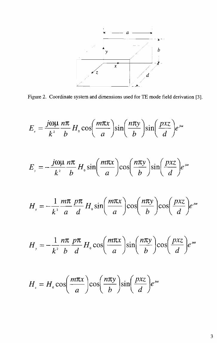
The TEmnp modes for a cavity resonator can be found in any elementary text and are
given below [2]. The expressions for electric and magnetic fields were derived from
Figure 2 with the z axis designated as the "direction of propagation". The existence of
perfectly conducting end walls at z=0 and z=d leads to the formation of standing waves,
i.e. no wave propagates within the cavity. The T E standing wave pattern within the
cavity is designated by the mnp subscript where m refers to variations of the fields in the
x direction, n in the v direction and p in the z direction.
2
a
/
/ /
/ d
_*._
Figure 2. Coordinate system and dimensions used for T E mode field derivation [3].
E = J'COLL nn ~V~~b
H^cos f mnx^
\ a J sin
f nny^ sin
' pxz^
V b J V d J jot
/COLL nn TT . ( mnx\
E =-+—?-—H sin k2 b ° V a J
cos sin ( pxz\ f nny^
\ b ) V d ) e j<at
H = 1 mn pn k2 a d
#„sin (mnx\
\ a J - cos
fnny^ cos
f pxz^
v b ) y d ) jo*
1 nn pn (mnx^ H = - — — ^ # o c o s
k2 b d \ a ) sin
(nny^ cos
(pxz^
\ b ) \ d jm
J
H =Hcos fmnx\ fnny^
cos \ a J
sin V o J
pxz V d j
i<m
3

where
k' = mn
\ a ) +
rnn\
The resonant frequency of the cavity is given by
1 i/mV rny ^n^ CO = - r = — + +
v*v p \d)
The preceding equations represent the electric and magnetic field components for
microwaves contained to a general rectangular cavity. However, this discussion is
confined to the dominant or TE101 mode as this mode represents the most desirable
condition for a microwave plasma applicator since the maximum electric field strength
is located along the central axis of the cavity as seen in Figure 3. For the TE101 mode,
these equations reduce to three non zero field components:
a fir.r\ ftr.7\ E =-j(D\iH0-sm
n
nx sin
U ) nz ,d
j(Ot
4

H =--H0sin d °
rnx^\
\a J
r COS
nz\ • e
jaii
V d)
H = Hn cos nx \
sin fnz\ jasi
V a ) v d )
Examining these three equations, w e see that the electric field has a maxima for x= a/2
and z=d/2, is in the y direction and becomes zero at the side walls as required by perfect
conductors [3]. The magnetic field lines lie in the x-z plane and surround the vertical
displacement current resulting from the time rate of change of Er There are equal and
opposite charges on the top and bottom walls because of the normal electric field ending
there. A current flows between the top and bottom, becoming vertical in the side walls.
This is analogous to a conventional resonant circuit, with the top and bottom acting as
capacitor plates and the side walls as the current path between them. This brings us full
circle to Figure 1 and the evolution of a cavity resonator from an LC circuit. The TE101
mode may be excited by a coaxially fed microwave probe inserted in the centre region
of the top or bottom face where Ey is a maximum or by a loop to couple to the maximum
Hx placed inside the front or back face. The best location for the probe or loop depends
on the impedance matching requirements of the microwave circuit of which the
resonator is a part. To couple microwave energy from a waveguide to the cavity, a hole
or iris at an appropriate location in the cavity wall is necessary. The field in the
waveguide must have a favourable component to excite the desired mode in the cavity
resonator.
5
Electric field
Magnetic field
U li n ll «i ll v
Side
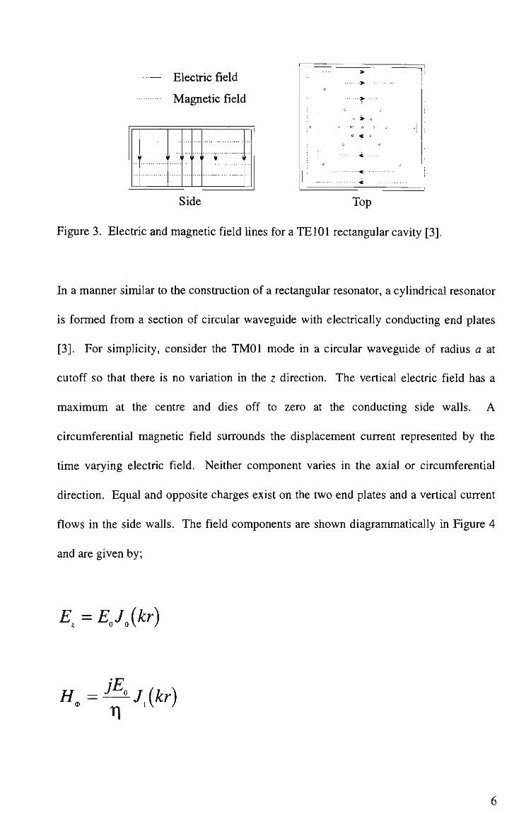
Figure 3. Electric and magnetic field lines for a TE101 rectangular cavity [3].
In a manner similar to the construction of a rectangular resonator, a cylindrical resonator
is formed from a section of circular waveguide with electrically conducting end plates
[3]. For simplicity, consider the T M 0 1 mode in a circular waveguide of radius a at
cutoff so that there is no variation in the z direction. The vertical electric field has a
m a x i m u m at the centre and dies off to zero at the conducting side walls. A
circumferential magnetic field surrounds the displacement current represented by the
time varying electric field. Neither component varies in the axial or circumferential
direction. Equal and opposite charges exist on the two end plates and a vertical current
flows in the side walls. The field components are shown diagrammatically in Figure 4
and are given by;
E. = E0J0(kr)
*1
6
k - p.. --2-405
a a
where the resonant frequency is
C0„ = 2.405
7(J£ a<sJ\ML
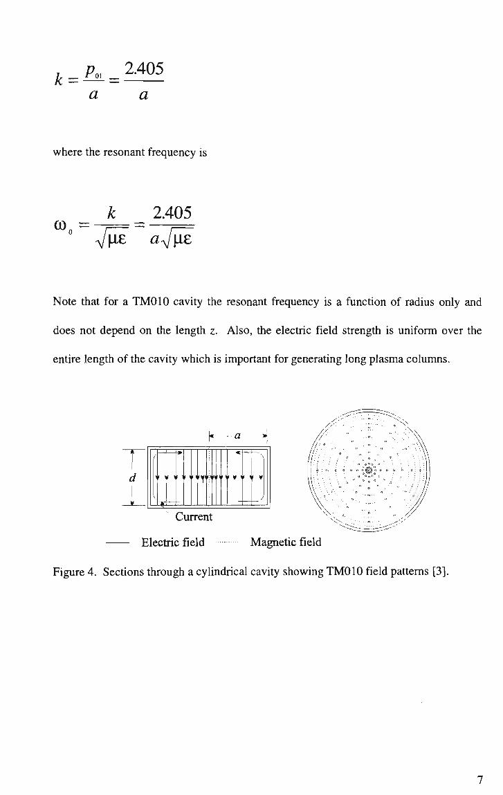
Note that for a T M 0 1 0 cavity the resonant frequency is a function of radius only and
does not depend on the length z. Also, the electric field strength is uniform over the
entire length of the cavity which is important for generating long plasma columns.
h~«-H t
I
\
1
*
f
-U-
— • » «- \
/
Current
Electric field Magnetic field
Figure 4. Sections through a cylindrical cavity showing T M 0 1 0 field patterns [3].
7

1.3 A Chronology of Applicator Development.
Research into ultra high frequency discharges in gases evolved from the development of
high power magnetrons used for radar purposes during the Second World War.
Equipment designed at the General Electric Research Laboratory, shown in Figure 5 and
reported on by Cobine and Wilbur [4], consisted of a coaxial applicator which produced
a torch like flame at atmospheric pressure from 1 kW developmental magnetrons
operating in the frequency range of 500-1100 MHz. The microwave energy was
coupled into a cavity which was then coupled to a coaxial section terminating in the
plasma torch. Tuning of the cavity was achieved by means of a tuning rod and the
coaxial section was adjustable to allow matching to the torch. The plasma gas flowed
out axially along the coaxial section. The torch was initiated by touching the inner
conductor with a carbon rod or a piece of insulated wire. Once the plasma was
established, the system was impedance matched by adjusting the length of the coaxial
section and the depth of penetration of the tuning slug. The efficiency of the torch
varied by as much as 60% depending on the plasma forming gas used and the discharge
tip had to be water cooled to prevent erosion. Plasma parameters were determined using
a 5.0 kW magnetron though it is not specified what the applicator arrangement was for
these tests.
8

Figure 5. The "Electronic Torch" of Cobine and Wilbur [4], 1951.
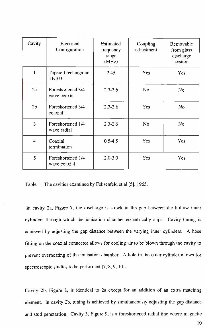
In 1965, Fehsenfeld [5] et al examined six microwave discharge cavities operating at
2450 MHz for use as spectroscopic light sources. The cavity assignments and
characteristics are given in Table 1. Medical diathermy units operating at 2450 MHz
and having a maximum output power of 125 W supplied the CW microwave power for
the cavities. These units were inexpensive and uncomplicated compared to government
surplus radar equipment. All of the cavities were designed to produce discharges in a 13
mm O.D. quartz tube.
Cavity 1, Figure 6, was the earliest cavity used [6] and consisted of a tapered waveguide
section with a slot cut into the narrow portion. The best operating characteristics were
obtained when the ionisation chamber was placed midway along the slot near the edge.
Coupling was achieved by an adjustable probe.
9
Cavity
1
2a
2b
3
4
5
Electrical
Configuration
Tapered rectangular TE103
Foreshortened 3/4
wave coaxial
Foreshortened 3/4
coaxial
Foreshortened 1/4
wave radial
Coaxial termination
Foreshortened 1/4 wave coaxial
Estimated frequency range (MHz)
2.45
2.3-2.6
2.3-2.6
2.3-2.6
0.5-4.5
2.0-3.0
Coupling
adjustment
Yes
No
Yes
No
Yes
Yes
Removable from glass discharge system
Yes
No
No
No
Yes
Yes
Table 1. The cavities examined by Fehsenfeld et al [5], 1965.
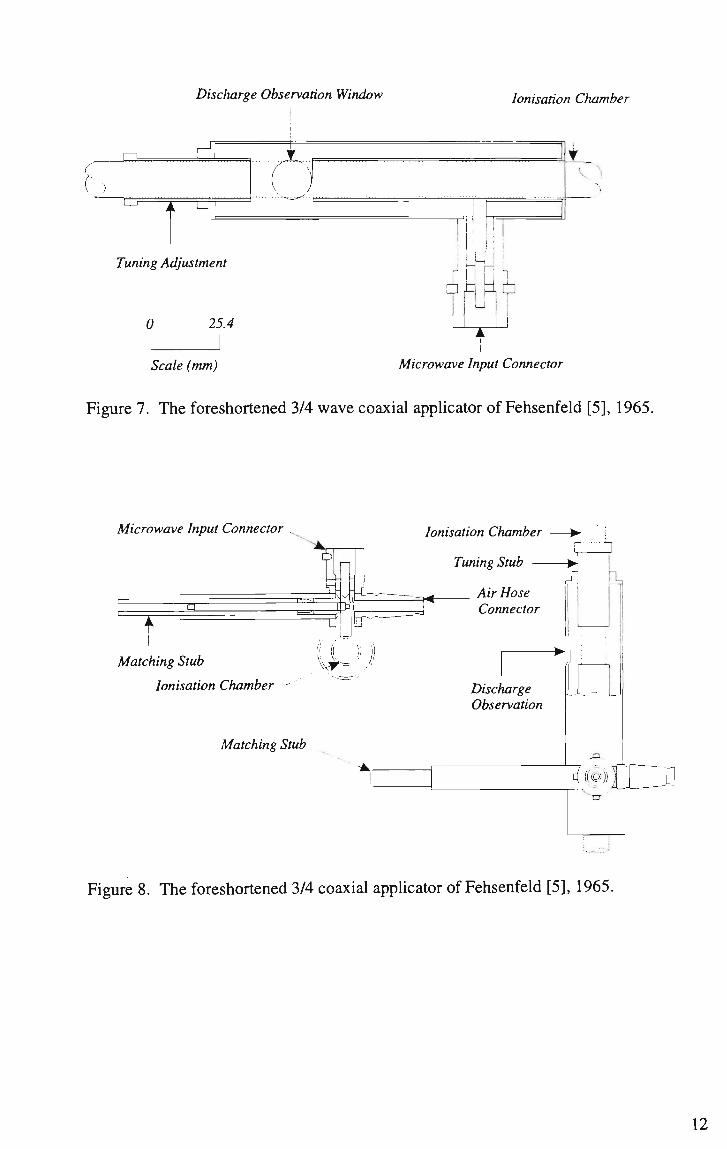
In cavity 2a, Figure 7, the discharge is struck in the gap between the hollow inner
cylinders through which the ionisation chamber eccentrically slips. Cavity tuning is
achieved by adjusting the gap distance between the varying inner cylinders. A hose
fitting on the coaxial connector allows for cooling air to be blown through the cavity to
prevent overheating of the ionisation chamber. A hole in the outer cylinder allows for
spectroscopic studies to be performed [7, 8, 9, 10].
Cavity 2b, Figure 8, is identical to 2a except for an addition of an extra matching
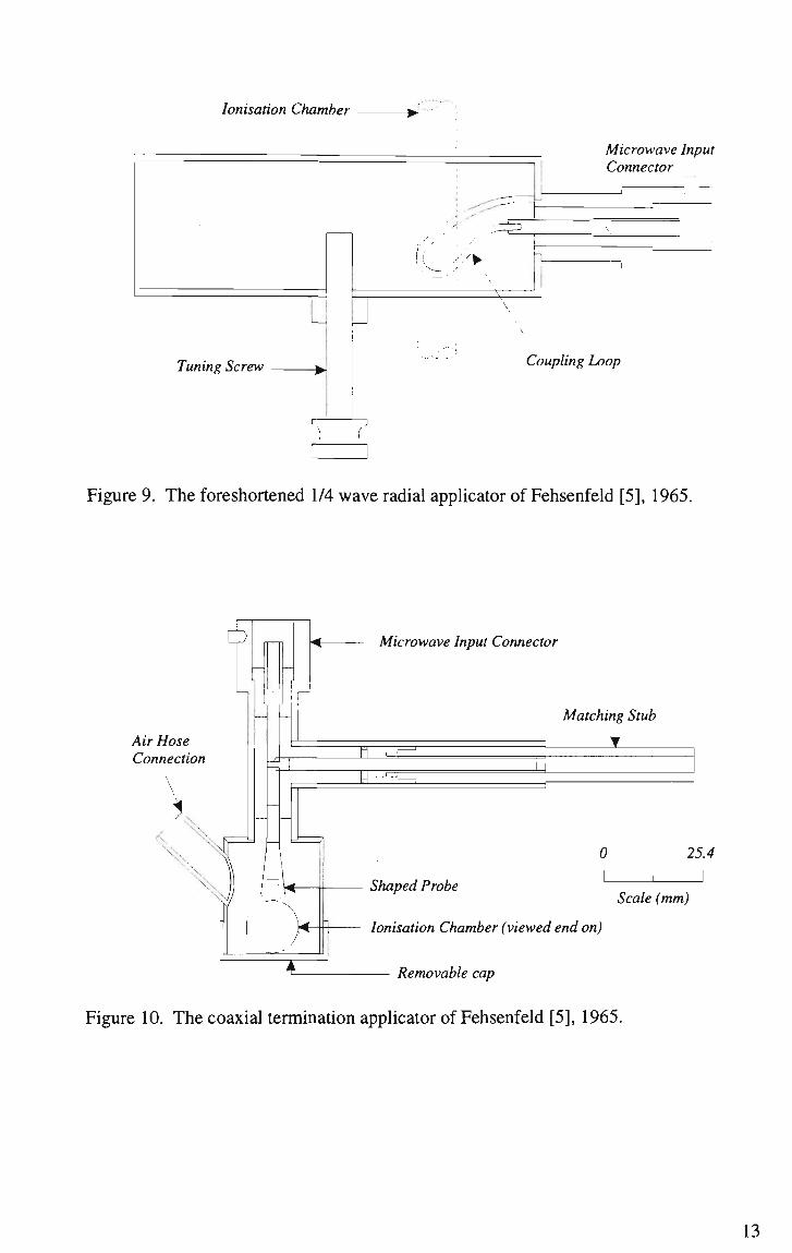
element. In cavity 2b, tuning is achieved by simultaneously adjusting the gap distance
and stud penetration. Cavity 3, Figure 9, is a foreshortened radial line where magnetic
10

3 0009 03254590 2
field coupling to the cavity is achieved via a large inductive loop. Air cooling of the
cavity is required to prevent the ionisation chamber from melting. The positioning of
the ionisation chamber hole was by trial and error to produce the most intense discharge.
In cavity 4 coupling is achieved via a matching stub located on the coaxial connector.
Supplementary coupling is achieved by adjustment of the shaped probe, see Figure 10.
Again air cooling of the ionisation chamber is necessary. Fehsenfeld draws attention to
the fact that this is not a resonant cavity in the sense of the other discharge cavities. He
goes on to say that the other cavities were designed to resonate at 2450 MHz and
perform over a limited band about this frequency whereas cavity 4 worked well over a
bandwidth greater than 1000 MHz.
Cavity 5, Figure 11, is a resonant cavity whose resonant frequency is adjusted by means
of a tuning stub and coupling by means of an adjustable slider. Cooling air for the
ionisation chamber is forced through a tube located in the body of the cavity.
Microwave Input Connector
Air Hose Connection
0 25.4 I i I
Scale (mm)
Tapered Rectangular Cavity Ionisation Chamber
Figure 6. The tapered waveguide applicator of Fehsenfeld [5], 1965.
11
Discharge Observation Window Ionisation Chamber
(
Tuning Adjustment
25.4
Scale (mm)
r ^
Microwave Input Connector
Figure 7. The foreshortened 3/4 wave coaxial applicator of Fehsenfeld [5], 1965.
Microwave Input Connector
>*.
T ^
Matching Stub
Ionisation Chamber
Matching Stub
Ionisation Chamber
Tuning Stub — Z
-=tr<-Air Hose Connector
n_
Discharge Observation
<#JF3]
Figure 8. The foreshortened 3/4 coaxial applicator of Fehsenfeld [5], 1965.
Ionisation Chamber
Tuning Screw
Microwave Input Connector
\
Coupling Loop
Figure 9. The foreshortened 1/4 wave radial applicator of Fehsenfeld [5], 1965.
6"
Air Hose Connection
<N
\\
Microwave Input Connector
r Matching Stub
>
25.4
Shaped Probe Scale (mm)
— Ionisation Chamber (viewed end on)
Removable cap
Figure 10. The coaxial termination applicator of Fehsenfeld [51, 1965.

Ionisation Chamber (viewed end on)
Tuning Stub
Microwave Input Connector
Removable Cap
Figure 11. The foreshortened 1/4 wave coaxial applicator of Fehsenfeld [5], 1965.
The two important things to note about all of these cavities is that they are coaxially fed
and that supplementary cooling of the ionisation chamber is necessary. In order to
increase the microwave power available for plasma generation, microwaves need to be
fed to the plasma cavity via waveguides. This overcomes the power handling limits of
coaxial cables. This is not necessarily an issue in the research lab but can be a problem
in an industrial environment where high levels of microwave power are needed for
applications such as welding of steel [11]. Swift describes a plasma torch [12] that is
coaxially fed and operates at power levels up to 2.5 kW. The unit operates at 2450 MHz
and is not based on a resonant cavity design but that of a coaxial applicator, Figure 12.
14

Tip- Plasma
, r 1
Coaxial -— Matching
Section
Shorting / Bridges
i !
u n.
From Microwave Source
Gas Fuel
J | Cooling
Figure 12. Schematic layout of a coaxial plasma torch as described by Swift [12], 1966.
The output of the magnetron is fed via a rigid 50 ohm coaxial line to the plasma torch
via a slotted line. Impedance matching of the plasma flame to the 50 ohm line is
accomplished by tuning the bridges in the two stub sections. A stream of cooling water
flows through the inner conductor of the matching element to cool the tip which screws
in and is interchangeable. The plasma gas flows axially along the inner conductor to the
tip in a similar manner to the electronic torch of Cobine and Wilbur [4]. The principal
difference between these two torches is the matching elements. Similarly though, the
plasma was initiated by an insulated rod with a pointed tungsten end which was placed
on the tip of the torch to produce the initiating spark.
A waveguide to coaxial transition, Figure 13, was the basis of the microwave discharge
system described by Murayama [13]. 400 W, 2469 MHz microwave energy was fed to
the coaxial waveguide via a rectangular waveguide. The discharge was generated on the
open end of the coaxial section where a water-cooled aluminium electrode was placed
15

on the tip of the inner conductor. Argon was used as the plasma forming gas and the
discharge was matched to the source by insertion of an inductive iris 63 mm from the
central axis of the coaxial waveguide. The discharge system was used for determination
of plasma parameters with the plasma being seeded with hydrogen, calcium and sodium
to facilitate the process.
Coaxial Waveguide
Rectangular Waveguide -
Flange
r . r ly-7
O , (jy-Tir--X
50v
<0
r-
Inductive Window ^ -o .- c
Discharge
- Aluminium Electrode
- Shorting Plate
w Inner Conductor s - Teflon Cylinder
Cooling Water _y Inlet and Outlet
Figure 13. Waveguide configuration of the discharge generator of Murayama [13],
1968.
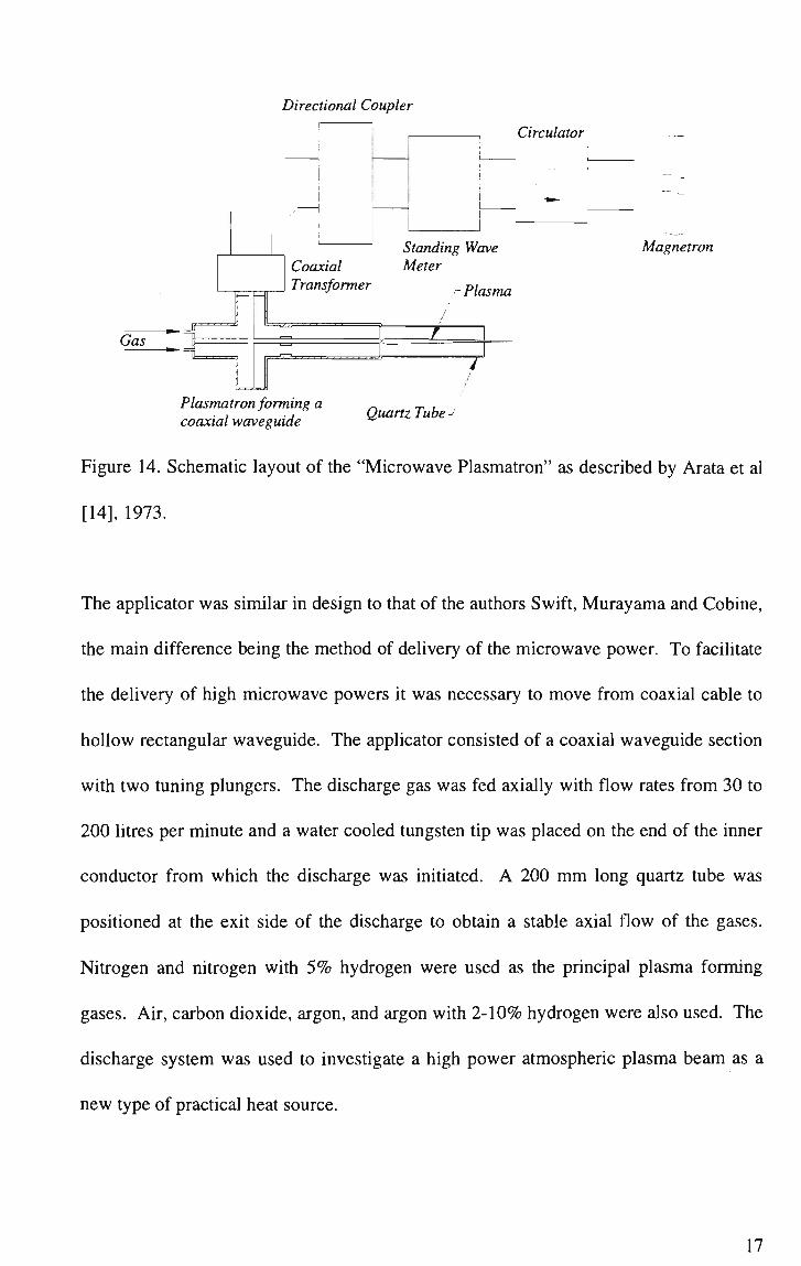
Work performed by Arata et al from 1973 to 1975 led to a series of four reports titled
"High Power Microwave Plasma Beam as a Heat Source". In Report 1 [14], subtitled
"Microwave Plasmatron in Nitrogen Gas", Arata et al used the arrangement given in
Figure 14 to deliver 3 kW at 2450 MHz of microwave power to a coaxial applicator via
rectangular waveguide.
16
Directional Coupler
._-= Gas m 1
"TL
Coaxial Transformer
Plasmatron forming a coaxial waveguide
Circulator
Standing Wave Meter
r Plasma
Quartz Tube
Magnetron
Figure 14. Schematic layout of the "Microwave Plasmatron" as described by Arata et al
[14], 1973.
The applicator was similar in design to that of the authors Swift, Murayama and Cobine,
the main difference being the method of delivery of the microwave power. To facilitate
the delivery of high microwave powers it was necessary to move from coaxial cable to
hollow rectangular waveguide. The applicator consisted of a coaxial waveguide section
with two tuning plungers. The discharge gas was fed axially with flow rates from 30 to
200 litres per minute and a water cooled tungsten tip was placed on the end of the inner
conductor from which the discharge was initiated. A 200 mm long quartz tube was
positioned at the exit side of the discharge to obtain a stable axial flow of the gases.
Nitrogen and nitrogen with 5% hydrogen were used as the principal plasma forming
gases. Air, carbon dioxide, argon, and argon with 2-10% hydrogen were also used. The
discharge system was used to investigate a high power atmospheric plasma beam as a
new type of practical heat source.
17

In Report 2, subtitled "Characteristics of 30 k W Plasmatron" [15], Arata et al examined
a 30 kW, 915 MHz plasma beam where the configuration of the plasmatron was
changed to the rectangular waveguide type in order to make the plasma axis parallel to
the electric lines of force.
Coupling Window
.— Tapered Waveguide
-i r, rv3
Copper Pipe for Water Cooling
Guide Copper Cylinder
Pyrex Tube Tuning Plunger
50 mm
7=>—;—-—c^sr Rectangular Cavity Resonator
Guide Copper Cylinder
Tangential Gas Inlet
Moveable Tungsten Ignition Wire
Figure 15. Cross sectional front view of the 30 k W plasmatron as described by Arata et
al [15], 1973.
Figure 15 gives the cross sectional front view of the plasmatron in detail. The main part
of the plasmatron was a water-cooled rectangular cavity resonator with dimensions
180x60x340 mm. A 40 mm I.D. Pyrex tube was inserted through the upper and lower
broad walls of the waveguide through which a tangential gas flow was introduced with
flow rates of 100-600 l/min. The protruding Pyrex tube was covered with water-cooled
copper cylinders to limit light emission and microwave leakage. The plasma was
ignited by inserting a tungsten wire into the Pyrex tube and sub matching was performed
18
by adjusting a tuning plunger at the end of the plasmatron. The primary matching
mechanism was an E-H tuner upstream from the plasmatron.
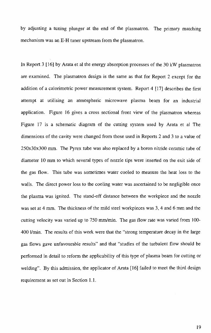
In Report 3 [16] by Arata et al the energy absorption processes of the 30 kW plasmatron
are examined. The plasmatron design is the same as that for Report 2 except for the
addition of a calorimetric power measurement system. Report 4 [17] describes the first
attempt at utilising an atmospheric microwave plasma beam for an industrial
application. Figure 16 gives a cross sectional front view of the plasmatron whereas
Figure 17 is a schematic diagram of the cutting system used by Arata et al The
dimensions of the cavity were changed from those used in Reports 2 and 3 to a value of
250x30x300 mm. The Pyrex tube was also replaced by a boron nitride ceramic tube of
diameter 10 mm to which several types of nozzle tips were inserted on the exit side of
the gas flow. This tube was sometimes water cooled to measure the heat loss to the
walls. The direct power loss to the cooling water was ascertained to be negligible once
the plasma was ignited. The stand-off distance between the workpiece and the nozzle
was set at 4 mm. The thickness of the mild steel workpieces was 3,4 and 6 mm and the
cutting velocity was varied up to 750 mm/min. The gas flow rate was varied from 100-
400 l/min. The results of this work were that the "strong temperature decay in the large
gas flows gave unfavourable results" and that "studies of the turbulent flow should be
performed in detail to reform the applicability of this type of plasma beam for cutting or
welding". By this admission, the applicator of Arata [16] failed to meet the third design
requirement as set out in Section 1.1.
19

Partially Tapered Waveguide
==QJ ^ ^
Copper Pipe -> /or Water Cooling
^ n^ -
Bf .
T"
— Tangential Gas Inlet
O-Ring
- Boron Nitride
- Guide Copper Cylinder
Rectangular Cavity Resonator
Moveable Tungsten ~~ Ignition Wire
Figure 16. Cross sectional front view of the 30 k W plasmatron used for cutting as
described by Arata et al [16], 1975.
Plasmatron
Work Piece —.
Pressure Gauge
Flow Meter
- Regulator
Shielding Box
Figure 17. Schematic diagram of the cutting system described by Arata et al [17], 1975.
20

In 1974, Asmussen et al [18] examined a cylindrical, variable length cavity operating at
2.45 GHz and 1.3 kW. Asmussen's cavity, shown in Figure 18, consisted of a 1.25 cm
I.D. quartz tube located on the axis of a 10.15 cm water cooled cylindrical cavity. The
quartz tube could be forced-air cooled when necessary. Small holes were cut into the
exterior walls of the cavity providing coaxial ports required for microwave diagnostic
measurements. Depending on the cavity mode excited, two adjustable loop coupling
antennae located in the side of the cavity, allowed the RF energy to be introduced into
the cavity. The cavity was tuned by means of a plunger that acted as a movable wall in
the plasma cavity system. RF energy is fed to the system coaxially and argon was used
as the discharge gas.
Holes for Coaxial Diagnostic Probes
Power Input Port
V-— \
v o
) M r\
Short-Length Adjuster
— Water Cooling ports
'— Screened Viewing Port
Quartz Ionisation Chamber
Figure 18. Cylindrical resonant cavity of Asmussen [18], 1974.
A cavity with the shape of a pillbox, as described by Beenakker [19], has found
applications in optical and atomic emission spectroscopy (OES and AES respectively)
and is represented schematically in Figure 19. The cavity consisted of a copper
cylindrical wall of I.D. 93 mm with a fixed bottom and a removable lid. The height of
21
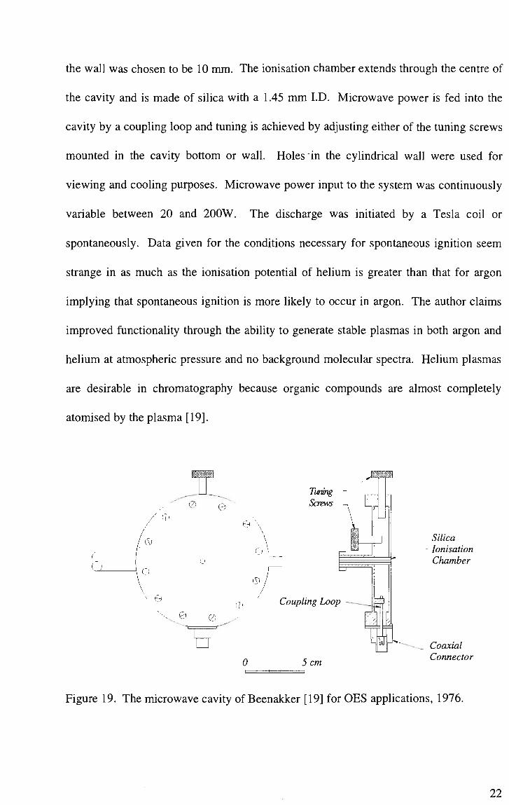
the wall was chosen to be 10 m m . The ionisation chamber extends through the centre of
the cavity and is made of silica with a 1.45 mm I.D. Microwave power is fed into the
cavity by a coupling loop and tuning is achieved by adjusting either of the tuning screws
mounted in the cavity bottom or wall. Holes in the cylindrical wall were used for
viewing and cooling purposes. Microwave power input to the system was continuously
variable between 20 and 200W. The discharge was initiated by a Tesla coil or
spontaneously. Data given for the conditions necessary for spontaneous ignition seem
strange in as much as the ionisation potential of helium is greater than that for argon
implying that spontaneous ignition is more likely to occur in argon. The author claims
improved functionality through the ability to generate stable plasmas in both argon and
helium at atmospheric pressure and no background molecular spectra. Helium plasmas
are desirable in chromatography because organic compounds are almost completely
atomised by the plasma [19].
Silica Ionisation Chamber
5 cm
Coaxial Connector
Figure 19. The microwave cavity of Beenakker [19] for O E S applications, 1976.
22

An atmospheric microwave discharge source known as a "Surfatron" was reported by
Moisan et al [20] in 1979. The device shown in axial cross section in Figure 20, is not a
resonant cavity but rather can be considered as a length of a coaxial transmission line. It
comprises two essential parts, the coupler and the excitation structure. The coupler is
constructed from a semi rigid coaxial cable terminated by a standard N-type coaxial
connector. An anodised aluminium plate is attached to the inner conductor and the
height or penetration depth of the plate relative to the inner coaxial tube determines the
coupling capacity. Minimising the reflected power is achieved by adjusting the height
of this plate. The research used 915 MHz, 700 W continuously variable microwave
power and for powers above 200 W, the surfatron was externally water-cooled.
LI =48.5 mm, 12=10 mm, g=3 mm. Dl=9 mm, D2=20 mm, 2b=6 mm.
. \ \ \ \ \ \ \ V V v
. \ \ \ \ y \ \ \ V \ \ \ -.
• \ \ \ \ . \ \ \ v \ 4^
?////////////'///. W . \ \ \ \ N
* •- V V , \ \ N
i^-r-Vri
^/>'A
y////.' //./••'/ /// v////y/////////y •/////,
/ /v-c
• /
Ll
N-Type Connector
Semi-Rigid Coaxial Cable
Coupler
2b] Dl
— 8 L2
D2
0 1 2 cm
Figure 20. The microwave surfatron of Moisan et al [20], 1979.
A small argon torch based on the surfatron is given in Figure 21. Small aluminium
wires, 1 mm were welded with this small torch. Other applications suggested by the
authors for the surfatron are as an excitation source for microsamples in O E S analysis,
23

as a spectroscopic light source for ultra violet study at pressures up to one atmosphere or
modified and used as a small welding torch.
Oxygen
~~i
i ' Argon
Figure 21. The plasma torch based on the surfatron of Moisan et al [20], 1979.
Bloyet and Leprince [21, 22] were granted two US patents dealing with a plasma
generator. The embodiment of both patents is identical, only the claims being different.
The plasma generator represented in Figure 22, is a hybrid coaxial/re-entrant cavity
design. Microwave energy is fed coaxially to a cylindrical re-entrant cavity. A hollow
metallic tube is passed coaxially through the centre of the cavity on the end of which the
plasma is generated and through which the discharge gas is passed. Ignition of the
plasma is accomplished by striking a spark between the end of the inner conductor and a
metallic rod brought into close proximity. The cavity was fed with 2450 MHz
microwave energy with power continuously varied from 15 to 500 W. The authors'
stress that this is not a resonant cavity confined to operation over a very limited
frequency range but a cavity with an operating bandwidth of order of 20% about the
24

nominal operating frequency. Matching is accomplished by adjusting the penetration of
a threaded rod located in the outer wall of the cavity.
Cylindrical Re-Entrant Cavity
Gas Inlet Hollow Metallic tube
Tuning Stub
N-Type Connector
Figure 22. Hybrid cavity design of Bloyet and Leprince [21, 22], 1984-86.
Moisan et al reported on a high power surface wave launcher [23] dubbed a "waveguide
surfatron". It consisted of both waveguide and coaxial line elements as seen in Figure
23. The microwave power is supplied from a generator to a rectangular waveguide
section terminated by a movable short circuit plunger. The coaxial section is attached
perpendicularly to the wall of the waveguide and its inner conductor extends into the
waveguide as a sleeve around the ionisation chamber forming a circular gap in the
immediate vicinity of the opposite wall. The waveguide surfatron design was first
proposed by Chaker et al [24] and has two matching mechanisms to effectively couple
microwave energy to the plasma column. Microwave powers up to 1.3 kW were tested
using this device with forced-air cooling of the ionisation chamber necessary for
25

microwave powers greater than 200 W . The I.D. and O.D. of the fused silica ionisation
chamber used was 10 and 47 mm respectively.
Coaxial Section •
Waveguide
Microwave Power Input •
y
Metal Sleeve /
Ionisation Chamber •
Figure 23. The waveguide surfatron of Moisan et al [23], 1987.
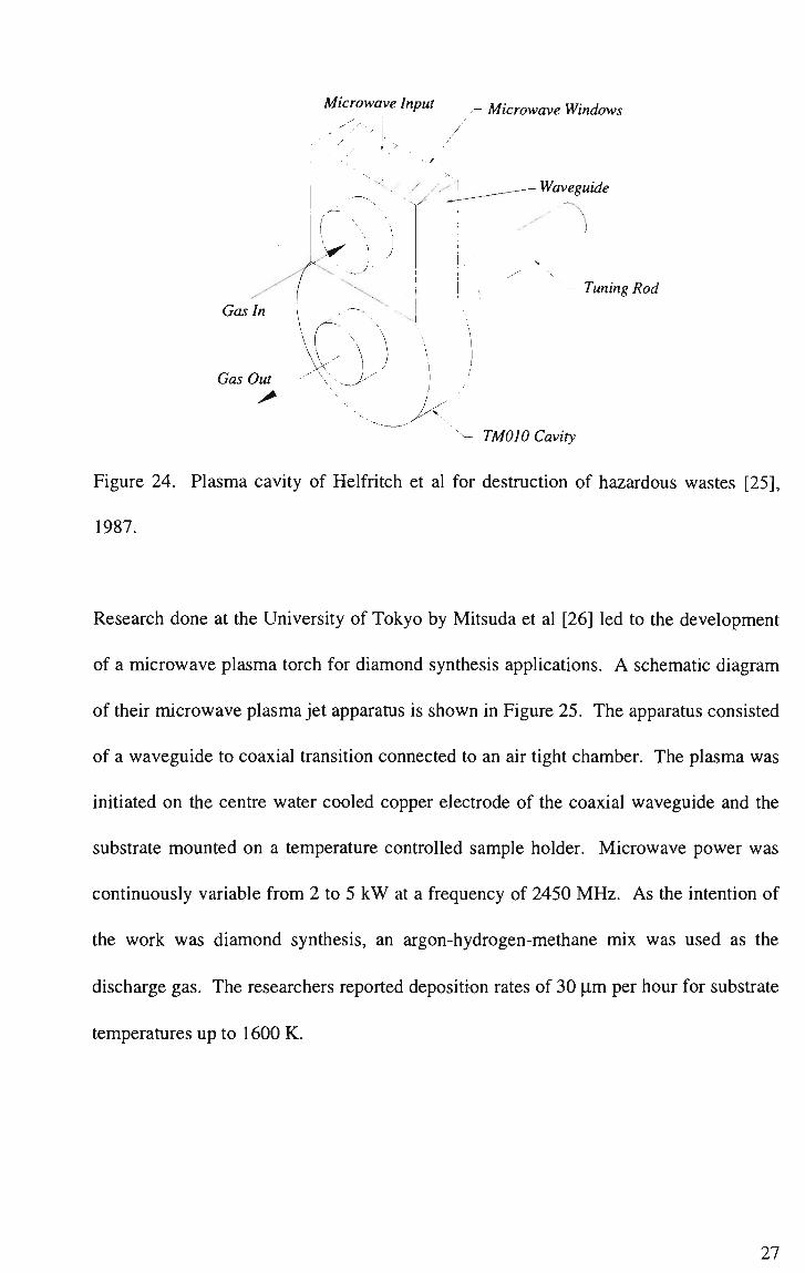
A TM010 resonant cavity was proposed by D. J. Helfritch et al for destruction of
hazardous wastes such as chlorinated hydrocarbons [25]. The article has very little
detail but gives the diagram shown in Figure 24. The cavity was constructed such that a
steel rod could be inserted into the cavity volume to allow for fine tuning to achieve
resonance. The author neglects to mention ignition methods or give any cross sectional
diagrams to indicate gas and waste flows. There is a claim of 1 kW of reflected power
for a forward power of 6 kW to achieve a plasma temperature of 4000 K but again, no
details are given. Both air and steam were used as the process gas.
Coaxial Plunger
Waveguide Plunger
Gap
26
Microwave Input Microwave Windows
Figure 24. Plasma cavity of Helfritch et al for destruction of hazardous wastes [25],
1987.
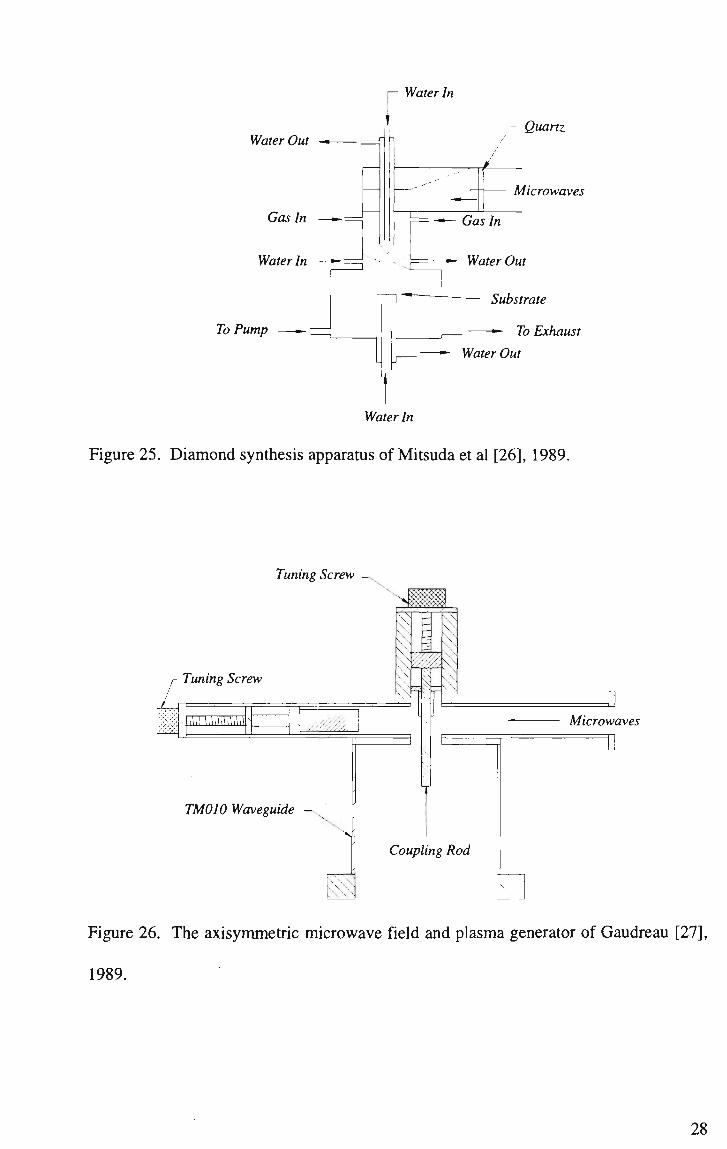
Research done at the University of Tokyo by Mitsuda et al [26] led to the development
of a microwave plasma torch for diamond synthesis applications. A schematic diagram
of their microwave plasma jet apparatus is shown in Figure 25. The apparatus consisted
of a waveguide to coaxial transition connected to an air tight chamber. The plasma was
initiated on the centre water cooled copper electrode of the coaxial waveguide and the
substrate mounted on a temperature controlled sample holder. Microwave power was
continuously variable from 2 to 5 kW at a frequency of 2450 MHz. As the intention of
the work was diamond synthesis, an argon-hydrogen-methane mix was used as the
discharge gas. The researchers reported deposition rates of 30 |Lim per hour for substrate
temperatures up to 1600 K.
27
r- Water In
Water Out
Gas In
Water In —*-='
- Quartz
Microwaves
Gas In
Water Out
To Pump
Substrate
,— — To Exhaust
—- Water Out
Water In
Figure 25. Diamond synthesis apparatus of Mitsuda et al [26], 1989.
Tuning Screw
Tuning Screw
gaum;
TM010 Waveguide - N
s
V ^
T
Coupling Rod
J] Microwaves
T]
Figure 26. The axisymmetric microwave field and plasma generator of Gaudreau [27],
1989.

In 1989, Gaudreau et al [27] were granted a U S patent for a microwave plasma
generator which is claimed to create an axisymmetric microwave field and plasma. The
device shown schematically in Figure 26, is essentially identical to that of Moisan's et al
[23]. The apparatus consists of a rectangular waveguide section through which a
conductive rod passes transversely and coaxially into a circular output waveguide.
There are matching elements on both the rectangular and circular waveguide sections.
The plasma apparatus is then mounted on a vacuum chamber in which experiments are
performed.
A microwave heating type plasma jet using a resonant cavity was investigated by Tahara
et al [28]. The subject of the research was a microwave plasma jet for space propulsion
that competes against the most widely used catalytic hydrazine thruster for attitude
control of artificial satellites. The device, shown schematically in Figure 27, consisted
of an aluminium TM011 resonant cavity and a 20 mm I.D. quartz ionisation chamber
located axially along the cylinder. Both the cavity and the ionisation chamber were
forced-air cooled. Matching was achieved by adjustment of a movable end wall. The
discharge gas was helium and microwave powers of 520 W at 2450 MHz were used.
Thrust was measured by the deflection of a target and thrust performance was evaluated.
The results obtained show that the thruster of Tahara et al [28] competes well against
the most widely used catalytic hydrazine thrusters for attitude control of artificial
satellites [29].
29

Discharge Plasma -
Centre Body -
Ionisation Chamber -
I'Q •'•'>' ''-"••' :
TJ
Pressure - Measurement Window
"C i :
'.. ~
'FOA
Working Gas In Resonant Cavity J COJ
Moveable Wall I 1 Microwave Input Window
Expanding Nozzle
0.1 m
Figure 27. The resonant cavity plasma jet for space propulsion of Tahara et al [28],
1990.
J. J Sullivan describes a resonant cavity design that requires no tuning mechanism and is
more stable in the US Patent # 4965540 [30]. The cavity was based on a cylindrical re
entrant design and the ionisation chamber extends axially though the centre of the cavity
as shown in Figure 28. Microwave power at 2450 MHz is fed coaxially to the cavity via
a coupling loop mounted through the cavity side wall. The claim of no tuning
mechanism relies on a low Q for the cavity and the coupling loop. The low Q for the
cavity is due to the increased conductance of a shorter plasma and that of the coupler
due to its lower reactance. A modification to the cavity is also proposed that allows for
liquid cooling to enable operation at higher powers. The modification consists of two
liquid cooled plates that attach to the top and bottom faces of the applicator and a
system of sealing rings and tubes to allow the coolant to circulate around a portion of
the ionisation chamber. The principal function of the cavity is as a spectroscopic light
source. No mention is given in the patent document of the microwave power level or
the discharge gas flow rates used.
30

Transparent Plasma
Figure 28. Schematic diagram of the spectroscopic light source proposed by Sullivan
[30], 1990.
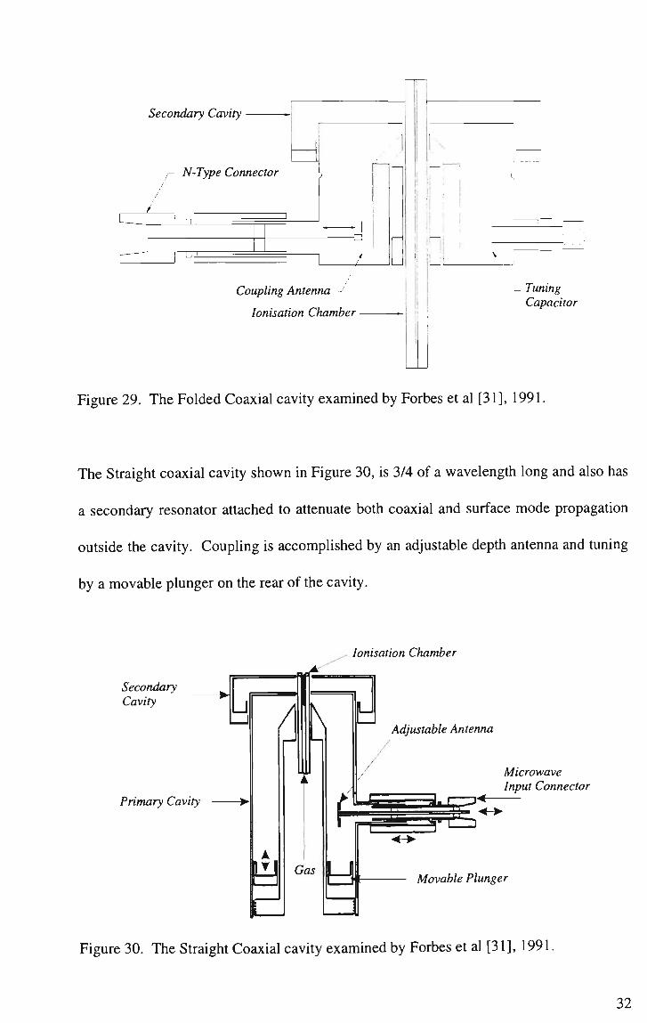
A comparison of microwave induced plasma sources was performed by Forbes et al in
JAAS [31]. The four cavities compared were a Folded coaxial, a Straight coaxial, an
Enhanced Beenakker TM010 and a Strip line source. The Folded coaxial cavity is a
modified surfatron-like structure and is shown in Figure 29. The folded coaxial line is
formed by the inner and outer walls of the tube (Figure 29-5) and is slightly shorter than
a quarter wavelength. The tapered tip coaxial conductor couples energy to the plasma
through the concentrating gap. Microwaves enter the cavity in a region where the local
electric field strength is a maximum. The second resonator placed at the output plane is
to reflect radiated microwaves back into the cavity. The discharge is maintained in a
quartz tube of I.D. 1 mm x O.D. 6 mm and is located axially within the cylindrical
cavity.
31
Secondary Cavity
Coupling Antenna -1
Ionisation Chamber
Tuning Capacitor
Figure 29. The Folded Coaxial cavity examined by Forbes et al [31], 1991.
The Straight coaxial cavity shown in Figure 30, is 3/4 of a wavelength long and also has
a secondary resonator attached to attenuate both coaxial and surface mode propagation
outside the cavity. Coupling is accomplished by an adjustable depth antenna and tuning
by a movable plunger on the rear of the cavity.
Ionisation Chamber
Secondary Cavity
Adjustable Antenna
Primary Cavity •
Microwave Input Connector
Movable Plunger
Figure 30. The Straight Coaxial cavity examined by Forbes et al [31], 1991.
32

The Beenakker cavity, shown previously in Figure 19, was modified to obtain a higher
coupling coefficient. This was achieved by the addition to the antenna of a movable
plate as used in the surfatron [20]. This eliminated the need for additional tuning at the
coupling loop and conventional frequency tuning could be achieved with a single screw.
The enhanced Beenakker cavity is shown in Figure 31.
Ionisation Chamber Antenna Plate
Figure 31. The Enhanced Beenakker cavity as examined by Forbes et al [31], 1991.
A schematic diagram of a strip line source is shown in Figure 32. The ionisation
chamber crosses the strip and is located at a region of maximum electric field strength
one quarter wavelength from the rear wall. At the other end of the strip, an adjustable
plate antenna couples microwave energy between a coaxial connector and the strip. A
capacitive tuner for adjusting the resonant frequency is located on the opposite side of
the strip with the strip being 3/4 of an electrical wavelength long. The plasmas were
initiated by inserting a nichrome wire attached to a small insulating rod into the
ionisation chamber. All four cavities described by Forbes are for OES applications and
33
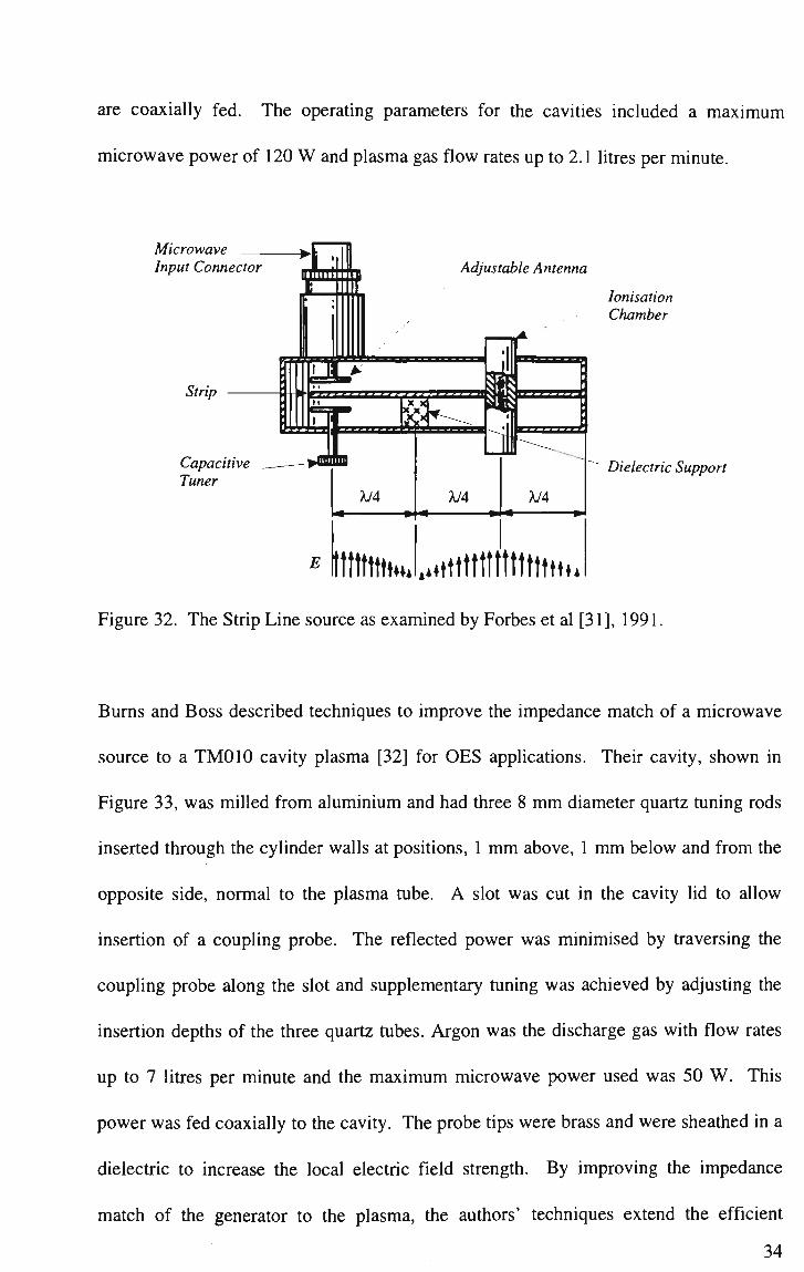
are coaxially fed. The operating parameters for the cavities included a maximum
microwave power of 120 W and plasma gas flow rates up to 2.1 litres per minute.
Microwave Input Connector Adjustable Antenna
Strip
Capacitive Tuner
lltltWtH.
Ionisation Chamber
..•ttttttttttttttm.
Dielectric Support
Figure 32. The Strip Line source as examined by Forbes et al [31], 1991.
Burns and Boss described techniques to improve the impedance match of a microwave
source to a TM010 cavity plasma [32] for OES applications. Their cavity, shown in
Figure 33, was milled from aluminium and had three 8 mm diameter quartz tuning rods
inserted through the cylinder walls at positions, 1 mm above, 1 mm below and from the
opposite side, normal to the plasma tube. A slot was cut in the cavity lid to allow
insertion of a coupling probe. The reflected power was minimised by traversing the
coupling probe along the slot and supplementary tuning was achieved by adjusting the
insertion depths of the three quartz tubes. Argon was the discharge gas with flow rates
up to 7 litres per minute and the maximum microwave power used was 50 W. This
power was fed coaxially to the cavity. The probe tips were brass and were sheathed in a
dielectric to increase the local electric field strength. By improving the impedance
match of the generator to the plasma, the authors' techniques extend the efficient
34

operating range of the microwave induced plasma and improve the detection limits and
sensitivities for a given amount or concentration of analyte.
h Argon _ i mmdM ^mrnh^
Plasma
Microwave Input — j (JTM "-1 !
I ^ Quartz Tuning Rods
i
Figure 33. The TM010 cavity of Burns and Boss [32], 1991.
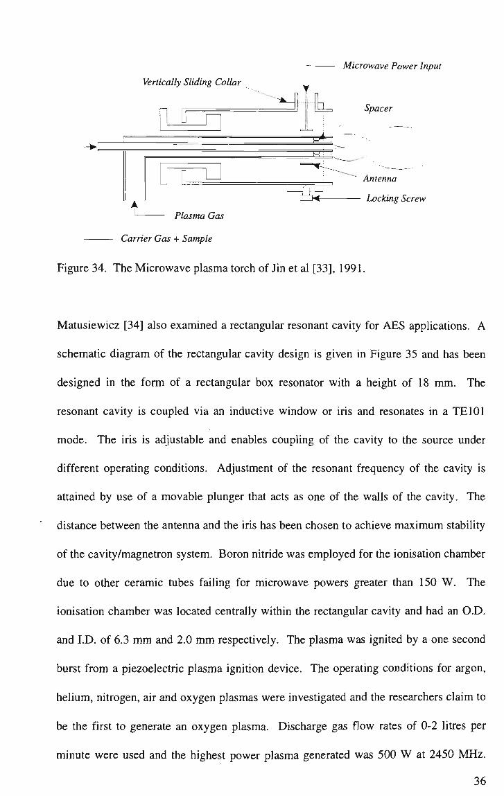
To overcome reported limitations such as the stability (and excitation capability) of the
resulting plasma being perturbed by small quantities of introduced foreign materials, Jin
et al [33] proposed the microwave plasma torch shown in Figure 34. The plasma torch
is similar in construction to the surfatron of Moisan [20], but has the ability to slide the
coupling antenna assembly along the length of the ionisation chamber. The ionisation
chamber is a concentric arrangement in which the plasma gas flows through the outer
tube and the carrier gas and sample flows along the inner. Microwave power is fed
coaxially and is continuously variable between 0 and 500 W at 2450 MHz. The torch is
designed for AES applications and detection limits of 1-50 ng/ml are claimed for most
of the elements studied.
35
Microwave Power Input
Vertically Sliding Collar
COM Locking Screw
Plasma Gas
Carrier Gas + Sample
Figure 34. The Microwave plasma torch of Jin et al [33], 1991.
Matusiewicz [34] also examined a rectangular resonant cavity for AES applications. A
schematic diagram of the rectangular cavity design is given in Figure 35 and has been
designed in the form of a rectangular box resonator with a height of 18 m m . The
resonant cavity is coupled via an inductive window or iris and resonates in a TE101
mode. The iris is adjustable and enables coupling of the cavity to the source under
different operating conditions. Adjustment of the resonant frequency of the cavity is
attained by use of a movable plunger that acts as one of the walls of the cavity. The
distance between the antenna and the iris has been chosen to achieve maximum stability
of the cavity/magnetron system. Boron nitride was employed for the ionisation chamber
due to other ceramic tubes failing for microwave powers greater than 150 W . The
ionisation chamber was located centrally within the rectangular cavity and had an O.D.
and I.D. of 6.3 m m and 2.0 m m respectively. The plasma was ignited by a one second
burst from a piezoelectric plasma ignition device. The operating conditions for argon,
helium, nitrogen, air and oxygen plasmas were investigated and the researchers claim to
be the first to generate an oxygen plasma. Discharge gas flow rates of 0-2 litres per
minute were used and the highest power plasma generated was 500 W at 2450 M H z .
36

The author claims superiority over the Beenakker cavity [19] in terms of electrical and
mechanical integrity, ease of tuning and extremely wide range of resonance and
coupling adjustments as well as excellent resistance to cavity detuning caused by
changes in plasma density with the introduction of wet aerosols.
Microwave Detector
1/2 Xg
3/8 Xg < •
£.
Magnetron
1 Inductive Window
if
Plasma
Plasma
Cavity
Ionisation Chamber
Gas
Figure 35. The rectangular cavity of Matusiewicz [34], 1992.
An International Patent submitted by Lucas and Lucas from The Welding Institute,
proposes a method for generating a plasma suitable for welding applications [35]. Two
applicator designs are proposed and both are coaxially fed and are based on a TM010
resonant cavity design. The first, shown schematically in Figure 36, consists of a
cylindrical cavity with an insertable slug that is transformed into a re-entrant cavity as
the slug is inserted. This increases the electric field strength in the region of the
discharge cavity. This ceramic button like cavity was located at the exit opening of the
resonant cavity, was circular in cross section and had a diameter of 7 mm and was 3 mm
high. A tungsten electrode is mounted within the cavity and the plasma gas was fed to it
37
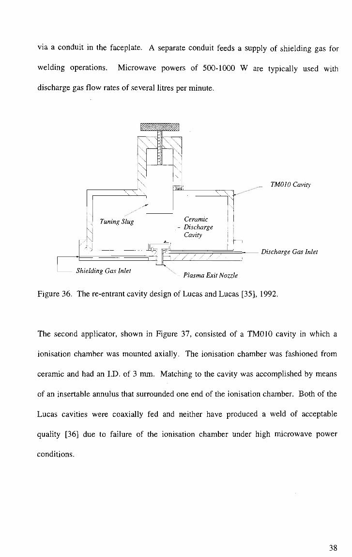
via a conduit in the faceplate. A separate conduit feeds a supply of shielding gas for
welding operations. Microwave powers of 500-1000 W are typically used with
discharge gas flow rates of several litres per minute.
\ \
Tuning Slug
Shielding Gas Inlet
ME
^ ^
Ceramic Discharge Cavity
^ s / / /. Plasma Exit Nozzle
TM010 Cavity
Discharge Gas Inlet
Figure 36. The re-entrant cavity design of Lucas and Lucas [35], 1992.
The second applicator, shown in Figure 37, consisted of a T M 0 1 0 cavity in which a
ionisation chamber was mounted axially. The ionisation chamber was fashioned from
ceramic and had an I.D. of 3 mm. Matching to the cavity was accomplished by means
of an insertable annulus that surrounded one end of the ionisation chamber. Both of the
Lucas cavities were coaxially fed and neither have produced a weld of acceptable
quality [36] due to failure of the ionisation chamber under high microwave power
conditions.
38

Discharge Gas Inlet -
Shielding Gas Inlet
Workpiece -^
\ \
TM010 Cavity
Ionisation Chamber
Workpiece Bias Supply
Nozzle
~~- Workpiece Bias Electrode
Figure 37. The TM010 cavity design of Lucas and Lucas [35], 1992.
Another application that can potentially gain from microwave induced plasma
technology is that of electrothermal space propulsion. Power has examined [37] the role
of microwaves in such an application and has constructed a TM011 operating at 915
MHz and 30 kW. The apparatus shown schematically in Figure 38, consists of resonant
cylindrical cavity with microwave and discharge gas feeds. A 5.7 T superconducting
magnet is included for implementation of a magnetic nozzle. The ionisation chamber is
fashioned from quartz for use at low powers and from alumina or boron nitride at high
powers. It has a 50 mm I.D. and is surrounded by a vacuum liner to minimise
conductive and convective heat losses. The vacuum liner provides an evacuated
annulus of 5 mm around the ionisation chamber. A moveable shorting wall or plunger
provides tuning capabilities and can be translated over such a distance as to allow for
tuning to TM011 or TM012 modes. At the time of writing, no plasmas had been
generated and the experimental work was limited to operation with a water load in place
of the cavity.
39
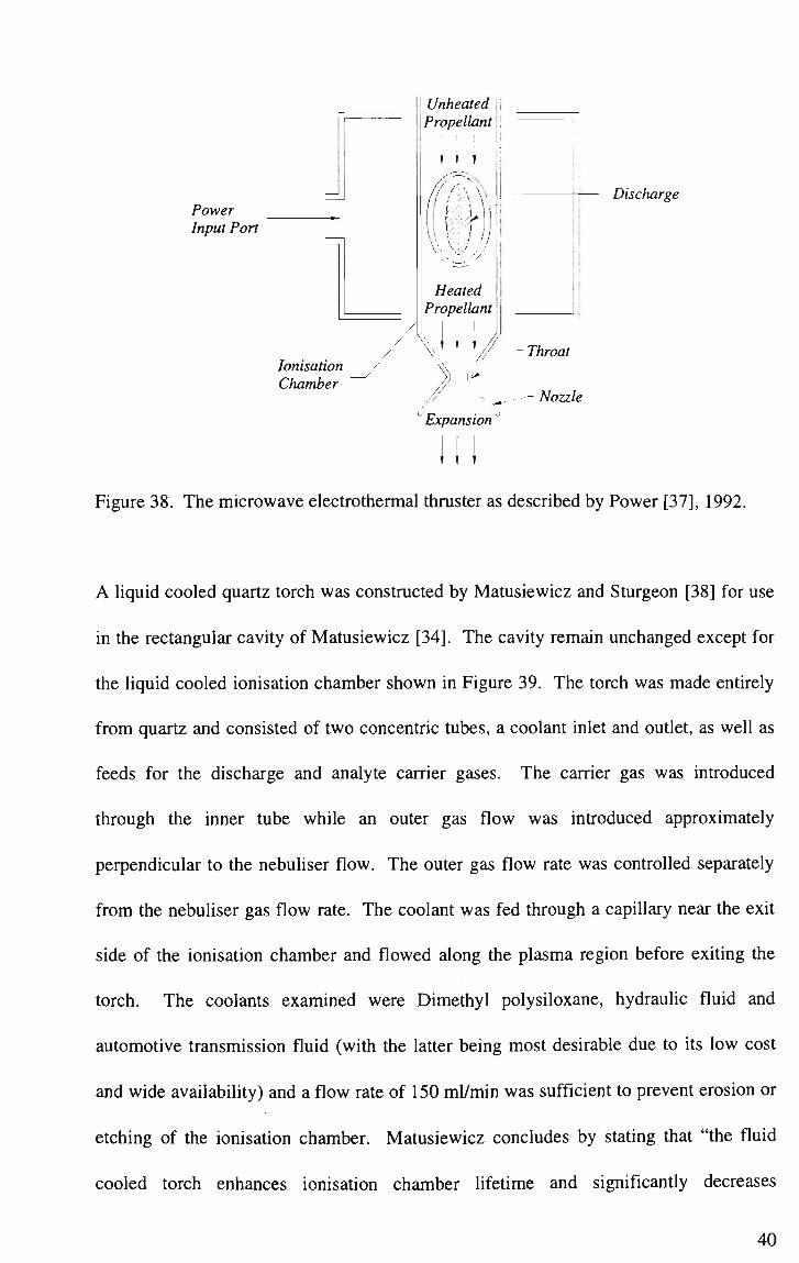
Power Input Port
—_
—
Ionisation Chamber
/ / y
Unheated Propellant
r i i
/fy-\
\\ at
Heated Propellant
i
- Throat
„- — M?zz
1 -
e
Discharge
L Expansion °
i t
Figure 38. The microwave electrothermal thruster as described by Power [37], 1992.
A liquid cooled quartz torch was constructed by Matusiewicz and Sturgeon [38] for use
in the rectangular cavity of Matusiewicz [34]. The cavity remain unchanged except for
the liquid cooled ionisation chamber shown in Figure 39. The torch was made entirely
from quartz and consisted of two concentric tubes, a coolant inlet and outlet, as well as
feeds for the discharge and analyte carrier gases. The carrier gas was introduced
through the inner tube while an outer gas flow was introduced approximately
perpendicular to the nebuliser flow. The outer gas flow rate was controlled separately
from the nebuliser gas flow rate. The coolant was fed through a capillary near the exit
side of the ionisation chamber and flowed along the plasma region before exiting the
torch. The coolants examined were Dimethyl polysiloxane, hydraulic fluid and
automotive transmission fluid (with the latter being most desirable due to its low cost
and wide availability) and a flow rate of 150 ml/min was sufficient to prevent erosion or
etching of the ionisation chamber. Matusiewicz concludes by stating that "the fluid
cooled torch enhances ionisation chamber lifetime and significantly decreases
40

erosion/ablation of the quartz tube surface, leading to a background emission spectrum
that is comparatively free of Si lines and molecular SiO bands in the UV-VIS and a
decreased continuum in the near IR [39]." The torch was ignited by inserting a section
of tungsten wire attached to a non-conducting handle.
Coolant In
_4. Outer
Coolant Out
Figure 39. The liquid cooled discharge torch of Matusiewicz et al [38], 1993.
A waveguide based field applicator [40] was used by Moisan et al for large diameter
plasma generation. The applicator consisted of a slotted antenna array bent into a
cylinder about an axis parallel to the slotted wall. This array is then housed within a
cylindrical chamber with flanges that acted as endplates as seen in Figure 40.
Microwaves were fed to the cavity via a tapered waveguide section and tuning was
accomplished using a standard waveguide plunger. The ionisation chamber was made
from quartz and was forced-air cooled with argon and helium being used as the
discharge gases. The microwave power supplied to the cavity was continuously variable
up to 1 kW at a frequency of 2.45 GHz.
41

Gas Inlet
"I -T-
Pressure Gauge
To Vacuum Aparatus
Flange
Ionisation Chamber
u
>.
Slot Array
Angular Waveguide
Flange
Input Taper
Standard Waveguide with Plunger
Figure 40. The waveguide based field applicator of Moisan et al [40], 1995.
1.4 Determination of Plasma Parameters.
Cobine and Wilbur [4] recorded an electron temperature ranging from 7.85E4 K at the
tip to 13.4E4 K near the inner electrode for a 350W atmospheric pressure discharge in
nitrogen. The measurements were obtained by means of a thin walled nickel tube (2.3
mm O.D., 0.76 mm wall) cooled by a strong stream of air passing through it. The probe
was located on the axis of the discharge and passed through the discharge at right
angles. The potential of the probe was measured relative to the inner conductor. The
authors report that reducing the power level by one half did not appreciably affect the
electron temperature (14.8E4) and the results generated are "at least of the correct order
of magnitude". The authors also make an estimation of the "flame temperature" of
between 1870-3740 K using buoyancy methods. This involves measuring the upward
deflection of a horizontally directed flame to determine the trajectory from which an
estimation of the temperature can be made. The plasma impedance was also measured
42
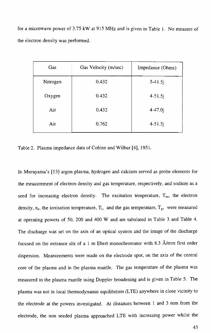
for a microwave power of 3.75 k W at 915 M H z and is given in Table 1. N o measure of
the electron density was performed.
Gas
Nitrogen
Oxygen
Air
Air
Gas Velocity (m/sec)
0.432
0.432
0.432
0.762
Impedance (Ohms)
5-41.5j
4-51.5J
4-47.0J
4-51.5J
Table 2. Plasma impedance data of Cobine and Wilbur [4], 1951.
In Murayama's [13] argon plasma, hydrogen and calcium served as probe elements for
the measurement of electron density and gas temperature, respectively, and sodium as a
seed for increasing electron density. The excitation temperature, Tex, the electron
density, ne, the ionisation temperature, T;, and the gas temperature, Tg, were measured
at operating powers of 50, 200 and 400 W and are tabulated in Table 3 and Table 4.
The discharge was set on the axis of an optical system and the image of the discharge
o
focused on the entrance slit of a 1 m Ebert monochromator with 8.3 A / m m first order
dispersion. Measurements were made on the electrode spot, on the axis of the central
core of the plasma and in the plasma mantle. The gas temperature of the plasma was
measured in the plasma mantle using Doppler broadening and is given in Table 5. The
plasma was not in local thermodynamic equilibrium (LTE) anywhere in close vicinity to
the electrode at the powers investigated. At distances between 1 and 3 mm from the
electrode, the non seeded plasma approached LTE with increasing power whilst the
43

seeded plasma deviated from LTE. Murayama interprets the deviation from LTE at
lower powers in the nonseeded plasma as being due to the inhomogeneity of the plasma.
Tex (K)
T,(K)
ne (IO14 cm"3)
Electrode
Spot
Non seeded
50 W
7900±100
7000±50
3.1+0.3
Non seeded
200 W
7500±90
6900±70
2.4±0.3
Non seeded
400 W
7100+90
6700±100
1.8±0.3
Electrode
Spot
Seeded
200 W
7400±90
6700±200
1.9±0.3
Table 3. Electrode spot plasma parameters as measured by Murayama [13], 1968.
Te- (K)
Ti(K)
ne(1014cnr3)
Central Core
Axis
Non seeded
50 W
7900±100
7400±70
6.1±0.7
Non seeded
200 W
6900±90
6800±200
2.0±0.6
Non seeded
400 W
6600±80
6600±100
1.5±0.4
Central Core
Axis
Seeded
200 W
6600+80
<6400
<1.0E14
Table 4. Central core axis plasma parameters as measured by Murayama [13], 1968.
44
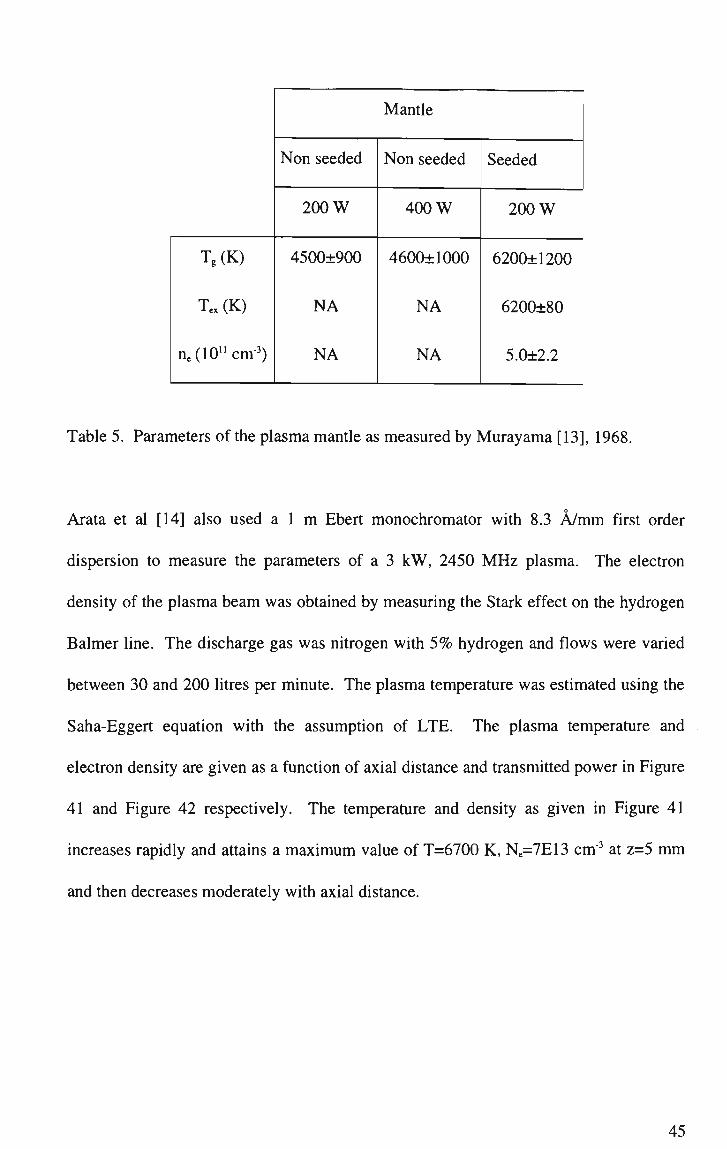
T,(K)
T« (K)
ne(10ncm-3)
Mantle
Non seeded
200 W
4500±900
NA
NA
Non seeded
400 W
4600±1000
NA
NA
Seeded
200 W
6200±1200
6200±80
5.0±2.2
Table 5. Parameters of the plasma mantle as measured by Murayama [13], 1968.
Arata et al [14] also used a 1 m Ebert monochromator with 8.3 A/mm first order
dispersion to measure the parameters of a 3 kW, 2450 MHz plasma. The electron
density of the plasma beam was obtained by measuring the Stark effect on the hydrogen
Balmer line. The discharge gas was nitrogen with 5% hydrogen and flows were varied
between 30 and 200 litres per minute. The plasma temperature was estimated using the
Saha-Eggert equation with the assumption of LTE. The plasma temperature and
electron density are given as a function of axial distance and transmitted power in Figure
41 and Figure 42 respectively. The temperature and density as given in Figure 41
increases rapidly and attains a maximum value of T=6700 K, Ne=7E13 cm'3 at z=5 mm
and then decreases moderately with axial distance.
45

N2+5V.H2 Plasma
Pt =1.8 kW
0 =56 l/min
r r . _1_ J L -l_
7.0 '£ u
r>
"o 6.0 -
H5.0 * z
--.JO
in
3.0 £
2.0 | in
1.0
I 2 3 U 5
Axial distance Z ( cm )
Figure 41. Plasma temperature and electron density as a function of axial distance,
Arata etal [14], 1973.
The plasma temperature and density increases nearly proportionally with power for
power levels >0.8 kW. The plasma temperature is given as a function of radial distance
and discharge gas flow rate for a 1.5 kW and 1.71 kW plasma respectively, in Figure 43
and Figure 44. As can be seen from these Figures, the plasma temperature is almost
constant for flow rates up to 200 l/min and the temperature decreases with radial
distance as would be expected. A standing wave meter in the rectangular waveguide
was used to measure the plasma impedance. Figure 45 and Figure 46 show the effect of
the plasma impedance on the transmitted power and discharge gas flow rate.
46

1.0 2.0 Transmitted power Pt ( kW )
Figure 42. Plasma temperature and electron density as a function of transmitted power,
Arata etal [14], 1973.
m 7.U O x •—
temp
erat
ure
CD
-8
E ro
K 6.0
1 0 0.1
Radial
N2+5'/.H2 Plasma Pt =1.5 k W <t> = 1-»1 l/min Z =12.5 m m
0.2 0.3 0.A distance ( cm )
Figure 43. Plasma temperature as a function of radial distance, Arata et al [14], 1973.
47
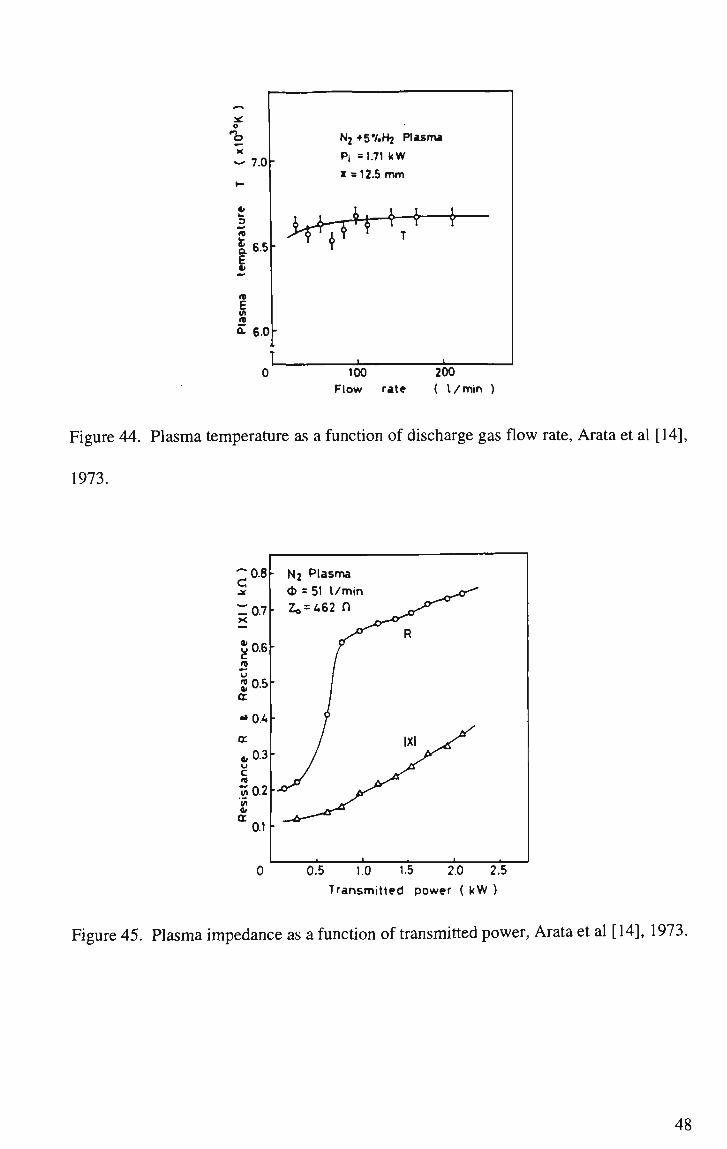
o
K
- 7.0
* |£6.5 E
ni
E in
« -- 6.0
N2+5V.H2 Plasma
Pi = 1.71 kW
i =12.5 m m
-L.
100 Flow rate
200 ( l/min )
Figure 44. Plasma temperature as a function of discharge gas flow rate, Arata et al [14],
1973.
ro.7 X
J 0.6 « TJ J 0.5 cc "-Or.
cr „0.3 u C it w0.2 «i « cr 0.1
- N2
0>: - Zo
•
•
•
—or
Plasma • 51 l/min --,62 n
• i
R
IXI y*^
0.5 1.0 1.5 2.0 2.5
Transmitted power ( k W )
Figure 45. Plasma impedance as a function of transmitted power, Arata et al [14], 1973.

700
S600h 4
£500
400
- 300
a 200
N, Plasma Pi «1.72 kW Z,-462 n
300 ?
-.200
* o
c.
cr
- t o o
100 200 Flow rate ( l/min )
Figure 46. Plasma impedance as a function of discharge gas flow rate, Arata et al [14],
1973.
Arata et al also examined the plasma properties of a 30 k W , 915 M H z plasmatron [16]
using spectroscopic methods. Plasma densities were again measured from Stark
broadening of the hydrogen Balmer line for various conditions by mixing various
percentages of hydrogen to the nitrogen (or argon) discharge gas. Assuming LTE the
temperature was then determined from the Saha equation. Good agreement was
obtained with plasma temperatures determined by measuring the relative intensity ratio
of hydrogen Balmer lines. Figure 47 shows there is little dependence of plasma
temperature or density on incident microwave power for a ionisation chamber diameter
of 40 mm. The temperature and density are about 6400 K and IE 14 cm3 for incident
powers between 10 and 25 kW. By reducing the ionisation chamber diameter to 20 mm,
the dependence of temperature and density on microwave power becomes more
pronounced as shown in Figure 48.
49

E o
t Tr.
c TJ
6.5
IMS'
N2 • 4.87.H2 Plasma
4 0 * PiP«
4^=200 l/tnin •fy^lO 1/min
•r-r-T
' - frl
0 5 10 15 20 25
Incident power f>. (kW )
Figure 47. Plasma parameters for a 40 m m ionisation chamber, Arata et al [16], 1973.
"E 4 u
>• 3
7.5
;7.0
N, +6 27.H2 plasma
20* pipe
4^,-152 t/min
4^,^10 l/min
6.5
L^ 0 5 10 15 20 25
Incident power Pt ( k W )
Figure 48. Plasma parameters for a 20 mm ionisation chamber, Arata et al [16], 1973.
The tendency of increasing temperature and density with decreasing ionisation chamber
diameter is shown in Figure 49 and Figure 50 for nitrogen and argon as the discharge
gases. This tendency supports the notion that a microwave plasma welder should be
based around a small diameter ionisation chamber. A 20 mm ionisation chamber
produced temperatures of about 6700 K and 7700 K in nitrogen and argon with
50
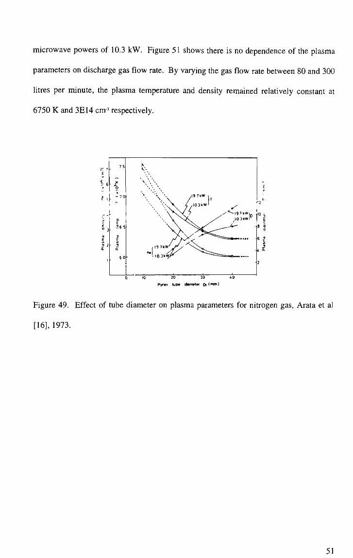
microwave powers of 10.3 k W . Figure 51 shows there is no dependence of the plasma
parameters on discharge gas flow rate. By varying the gas flow rate between 80 and 300
litres per minute, the plasma temperature and density remained relatively constant at
6750 K and 3E14 cm3 respectively.
r "* E
D J-
75
70
e 26 5
50
,!9 7kW
20 10
Pyrta tube <famttcr Dl (n*n)
-0
Figure 49. Effect of tube diameter on plasma parameters for nitrogen gas, Arata et al
[16], 1973.
51
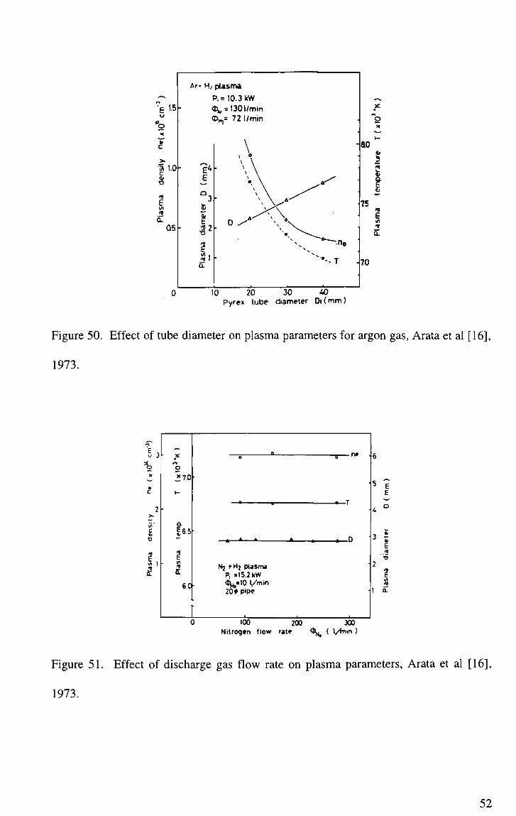
• E «
tl
c
fl.0 c t) lfl
E in
n a. Q5
Ar* H/ plasma
Pi = 10.3 kW <t»„ = 130 l/min <DM,= 72 l/min
g-4 E
3-
I 32 •A ,
<v 1
-ao
•», -T
"o
5
75 E m a
70
10 20 30 40 Pyrex tube diameter Dt(mm)
Figure 50. Effect of tube diameter on plasma parameters for argon gas, Arata et al [16],
1973.
3-
c d
Ir |
• O
37.0
Q.
|6.5
n E i/i
t E 6.0
o o
Nj I-HJ plasma P, -15.2 kW cfi sio l/min 20 # pipe
f
g n-
x * n '
•
100 200 300 Nitrogen tlow rale c|^ ( l/min )
-
E
a
E <« •5 2
I a
Figure 51. Effect of discharge gas flow rate on plasma parameters, Arata et al [16],
1973.

s:
8.0 w 3
7.5
N..H, plasma *„, z 321 t/min
•» s 20 l/min
a a.
7.0'
6.5
0
r."^"'
— - • * • '
^/ 4mm*
5mm*
8 mm nozzle
-x~ 20 pipe
10 15 20 Incident power Pj (kW)
Figure 52. Temperature dependence on incident power and nozzle diameter, Arata et al
[17], 1975.
©
I 80 ti
3
O u «l
a * 7-5 a E M O a.
7.0
N..H, plasma
4mm* nozzle P, :15kW
$„,-. 20 l/min
200 300 -.00
Gas flow rate $ (l/min)
Figure 53. Temperature dependence on gas flow rate and nozzle diameter, Arata et al
[17], 1975.
Arata et al [17] also examined the plasma temperature as a function of incident power
for various nozzle diameters, Figure 52 and gas flow rates for various nozzles, Figure
53. In each case, the temperature is greater for a smaller nozzle diameter as would be
expected from thermodynamic principals.
1.5 Summary of Literature Review.
Applicators for generating microwave plasmas can be broadly separated into two
groups. These are coaxial and cavity applicators. The coaxial applicators were first
used in the early 1950's and were generally low power devices that were coaxially fed
microwave power. In order to minimise degradation of the centre conductor or
discharge tip, materials such as copper and tungsten were used in conjunction with
water cooling techniques. This kept the tip cool enough so that erosion did not occur.
To generate plasmas with higher powers, it was necessary to use metallic waveguides to
deliver the microwave power instead of coaxial cables. The result was an applicator
that required a waveguide to coaxial transition and is well illustrated by Figure 13.
Coaxial cables however, have some benefits over waveguides, such as flexibility of the
cable and reduced bulk. Bulk is especially important as the microwave frequency is
reduced. For example, at 2450 MHz, a TE10 waveguide has internal dimensions of 43
x 86 mm whereas at 915 MHz, these dimensions increase to 120 x 240 mm. Coaxial
cables capable of carrying very high microwave powers are now available and are being
used in the generation of microwave plasmas [37]. Though these cables are not small,
they are still flexible. The cable used by Power [37] measured 12.5 cm in diameter and
was rated at 32 kW of CW microwave power at 915 MHz. The cut-off frequency was
960 MHz and the attenuation was less than 0.05 dB over a 5 m length. Using such a
54
high power rated cable should allow the generation of a microwave plasma using the
coaxial techniques described in Section 1.3. These techniques do not require the
ionisation chamber used in cavity applicators. The ionisation chamber is prone to
failure due to absorption of microwave energy with increasing temperature but does
produce a collimated plasma beam essential for applications such as high quality
welding.
The first resonant cavity applicators were coaxially fed devices for operation at low
powers [5]. As the power input to these devices was increased beyond a few hundred
Watts it became necessary to provide supplementary cooling of the ionisation chamber
to prevent tube failure. Many researchers [5, 18, 19, 23, 28, 40] used forced-air cooling
techniques to extend the life of their ionisation chambers. Arata et al [17] used water
cooling techniques to show that the plasma heat loss to the walls of a 20 mm ionisation
chamber was negligible due to the helical flow of gas producing a virtual cold wall.
Sullivan makes reference to water cooling in Reference [30]. In his design the annulus
of water surrounds only part of the ionisation chamber and is a mere 0.1 mm thick. He
goes on to say that water coolant can be replaced by air flow if desired. The implication
here is that water cooling is not necessary in his design though it may just be a case of
operating at low enough powers to ensure the ionisation chamber is in no danger of
failing. No information is given on operating parameters in the patent text. In fact not
all designs require supplementary cooling of the ionisation chamber as shown in
Reference [16]. If the I.D. is large enough then a gas wall can be formed that limits the
contact of the plasma with the walls of the ionisation chamber. Unfortunately, a large
I.D. also means a large diameter plasma which is not desirable for welding studies. To
overcome the large diameter plasma a nozzle arrangement can be used [17]. A nozzle
55

serves two functions; firstly it reduces the diameter of the plasma beam and secondly it
can increase the plasma temperature by adiabatic compression. Both are desirable
properties for optimal welding performance. Nozzles also have some undesirable side
effects when it comes to welding. The nozzle erodes with time due to contact with the
plasma and the erosion products contaminate the welding process. Also, as the nozzle
erodes, the plasma exit orifice increases in size leading to reduction in weld quality from
a larger heat affected zone.
Resonant cavity applicators can be subdivided into various groups. These are
rectangular, cylindrical, waveguide and waveguide field applicators. The literature
seems to favour cylindrical cavities possibly due to the ability to have a plasma greater
in length than a quarter wavelength though this may not be desirable for all applications.
The waveguide field applicator of Moisan et al [40] appears to be unique in the
literature and has applications in large area plasma generation. Throughout the literature
there has been a correlation between ionisation chamber diameter and microwave
power, i.e. high microwave powers are associated with tubes of large I.D. Those
cooling techniques in the literature have dealt with large diameter ionisation chambers
and high powers or with low powers and small diameter tubes. Plasma operation with
small diameter ionisation chambers and high microwave powers have not been
examined due mainly to the difficulty in maintaining a high temperature plasma in
contact with the walls of the ionisation chamber without failure.
Plasma parameters have been measured for both coaxially generated [4, 13] and cavity
generated plasmas [14, 16, 17]. For the three coaxially generated plasmas reviewed, the
maximum microwave powers used were 350 W with a nitrogen discharge gas flow
56

velocity of approximately 1 m/s, 1.8 k W with nitrogen gas flow rates of up to 200 l/min,
and 400 W with argon gas flow rates of 11 g/min (~ 9 litres/min). For cavity generated
plasmas, microwave powers of up to 20 kW were used with nitrogen discharge gas flow
rates from 80 to 300 l/min. None of the temperature measurement methods used a direct
means of measuring temperature. Instead, assumptions about the state of the plasma
were made and then temperatures determined using these assumptions. The assumption
was that the plasma was in a state of local thermodynamic equilibrium allowing
temperatures to be determined from densities using the Saha-Eggert equation. The
temperatures derived were generally between 5000 to 8000 K regardless of the
applicator used or the microwave frequency or power level. In some cases [4, 13], the
temperatures recorded were spot temperatures and are not indicative of the thermal
profile of the plasma. There has also been no systematic investigation to fully quantify
plasma parameters over the complete operating range of applicator variables.
1.6 Conclusion.
This literature survey enumerates applicator development since the late 1940's and has
examined the ways in which a plasma can be generated using microwaves. Though it
does not cover all the work done by all researchers, it does cover all major applicator
types and important advances in the science of generating microwave plasmas at
atmospheric pressure. Those applicators designed to operate at reduced pressures are
not covered nor are those that use methods other than microwaves for plasma generation
as they are outside the scope of this thesis.
57

Applications for microwave induced plasmas are diverse and research for use as a heat
source or in space propulsion is detailed. By far the most interest for microwave
induced plasma applications comes from the spectroscopy community. Microwaves are
capable of generating high power, inert, stable and luminous plasmas at atmospheric
pressure. Inert gases are preferable to molecular gases because of the absence of a
background molecular spectrum. Using a large diameter ionisation chamber (or cooling
of the tube) also leads to reduced atomic and molecular emission since ablation of the
tube walls does not occur from contact with the plasma thereby increasing sensitivity
and reducing detection limits.
As mentioned in the introduction, a microwave induced plasma applicator capable of
welding sheet steel requires: i) a well collimated beam with a diameter as small as
possible, ii) a plasma beam with sufficient power to rapidly melt steel, iii) a discharge
gas flow rate low enough to ensure molten metal is not ejected from the weld pool, iv)
and the ability to shape the cross section of the plasma beam. A small diameter, well
collimated beam can be most easily produced by use of a ionisation chamber that has a
small inside diameter. This translates to using a cavity applicator, as there is no
provision for a ionisation chamber in a coaxial design. To rapidly melt steel, high
microwave powers are necessary. Table 6 gives ionisation chamber I.D. and the
microwave power regime for those references cited in Section 1.3 that require a
ionisation chamber. As can be seen from this Table, high microwave powers combined
with small diameter ionisation chambers are virtually absent from the literature. It is
this area of research that this thesis embodies as well as application of microwave
induced plasmas to welding of sheet steel. The applicator must be able to operate
efficiently at low discharge gas flow rates and have the ability to change the shape of the
58

cross section of the plasma beam. To date, all plasma beams reported in the literature
are of circular cross section. The ability to shape the plasma beam is advantageous
when it comes to welding because one applicator can serve the purpose of preheating
the metal, melting and heat treatment of the weld in one pass. A similar method
employed currently in industry is known as multi cathode TIG (tungsten inert gas).
Here, separate TIG cathodes (and power supplies) provide, preheating, melting and heat
treatment functions. Both The Welding Institute (TWI) England and the Japanese
Welding Research Institute (JWRI) in Japan have examined microwave generated
plasmas as a heat source for cutting applications [35, 17]. Neither however, have
published any data on welding research using microwave plasmas. TWI have been
limited to low powers due to ionisation chamber failure [36] and JWRI possibly by the
high gas flow rates necessary to sustain the plasma in their applicator. As previously
mentioned, high gas flow rates expel the metal from the weld zone once it has become
molten so instead of welding a cutting action is initiated.
Application of microwave plasmas to welding and small diameter ionisation chambers
combined with high microwave powers are not covered in the literature. As such there
has been no systematic investigation to quantify plasma parameters or weld quality over
the range of applicator variables. This thesis will rectify these deficiencies.
59

Power (kW)
Tube I.D.
(mm)
Small
<5 mm
Medium
5<d< 10 mm
Large
> 10 mm
Low
P<0.5
19,28,31,32,
34,35
20,23
5, 18
Medium
0.5<P<1.5
35,38
20,23
18
High
P>1.5
17
15,16,37
Table 6. Ionisation chamber diameter and microwave power for selected references.

CHAPTER 2. EXPERIMENTAL DESIGN, EQUIPMENT AND PROCEDURES.
2.1 Introduction.
The goal of this thesis was to develop a microwave generated plasma device that could
produce a beam of plasma capable of welding sheet steel using off the shelf components
where possible. This chapter describes the componentry used to generate and measure
microwave radiation. It also describes the ancillary equipment used in the course of
experimentation but does not cover the design of the plasma beam applicator. This is
left for Chapter 3. Figure 54 represents diagrammatically those components of the
experimental apparatus that are detailed in Chapters 2 and 3.
Gas In
Output to Power Meter
1. Magnetron
Output to Power meter
Circulator with Water load
n Aid-
Slotted Section
Dual Port Directional Coupler
3 Stub Tuner
&<#' ,«.-*
Plasma Out
Sliding Short Circuit
CW>Y' ,.-*
Figure 54. Diagrammatic representation of experimental apparatus.
61

Also covered in this chapter is the experimental procedure required for prolonged and
safe operation of the microwave equipment. In the interest of safety and due to the
extreme voltages and high microwave powers used, it was occasionally necessary for
some procedures to be performed in conjunction with another doctoral student. It is
made clear in the text where data has been generated collaboratively.
2.2 Pulsed Power Supply.
The first microwave power supply used was constructed in-house by the Microwave
Applications Research Centre, a wholly owned company of the University of
Wollongong. It was rated at approximately 1.5 kW and produced microwave power
pulsed at the line frequency of 50 Hz. This was satisfactory for preliminary
experimentation but it became quite clear that continuous power was necessary to
prevent the plasma from extinguishing and then re-igniting 50 times per second. This is
important since the plasma was first initiated by use of a conducting wire inserted into
the high electric field region of the applicator. If the plasma then extinguishes, the wire
needs to be re-inserted so that the wire becomes a consumable and/or contaminant since
it must be left in place for continued plasma generation.
The shock wave from the expanding plasma front created a moderately loud bang when
the plasma was first initiated. At 50 Hz, the 50 bangs per second were so noisy that the
shock front could be quite plainly seen on an oscilloscope fitted with a microphone.
The noise was completely eradicated by using continuous microwave power.
62

2.3 Continuous W a v e Power Supply.
Conventional power supplies [41], used to drive high power continuous wave or CW
magnetrons, utilise a step-up transformer with its secondary high voltage output
connected to rectifiers to provide the dc high voltage for the magnetron. Although the
ideal power supply would provide a current source, present conventional design
provides a voltage source applied to the magnetron. In order to control the microwave
output power with a voltage source applied to the magnetron, it is necessary to adjust
the magnitude of the current in its electromagnet.
Funding was obtained to purchase a Spellman High Voltage Corporation MG10
switched mode 10 kW magnetron power supply. Along with the power supply, a
National YJ1600 6 kW water cooled magnetron, launcher and circulator were
purchased.
To evaluate power supply and magnetron operating conditions, filament current, anode
voltage, anode current as well as output power of the power supply were all monitored.
To evaluate the performance of the system, hour meters were implemented to log
magnetron hours as well as power supply high voltage hours.
Spellman [41] claims that high frequency, 20 kHz, resonant invertor technology
provides the following benefits over conventional magnetron supplies;
• A true current source for the magnetron allows direct control of the magnetron output
power and provides inherent current limiting capability during a fault condition.
63

• L o w output ripple current is obtained without the need for the energy storage filter
components that could damage the magnetron in case of an arc or fault condition. No
large values of capacitance or inductance are used.
• Reduced line frequency ripple is achieved through fast responding current feedback
circuits.
• The output power can be shut down in less that 30 microseconds after a fault signal is
received and then reapplied according to a pre-set programme. The fast response
prevents magnetron damage when signals are applied from fault monitor circuits
such as (TC-1) or arc detectors.
• The output power can be controlled through a remote interface. Inputs may be
derived from external sources such as temperature probes or a directional
coupler/detector that provides an indication of excessive reflected power.
• Size and weight reduction of the power supply (by a factor of five) is achieved
because high frequency invertor technology allows the use of small and light
magnetic components.
• Magnetron stress is minimised through automatic ramping of the anode voltage and
current.
• Remote and local control of the output powers are programmable, e.g. through a
PLC.
2.4 Circulator.
A circulator or isolator is a three port microwave device that is used to prevent reflected
microwaves from coupling to the magnetron antenna. In operation, magnetised ferrites
in the circulator employ Faraday rotation to couple microwaves incident on port 1 to
64
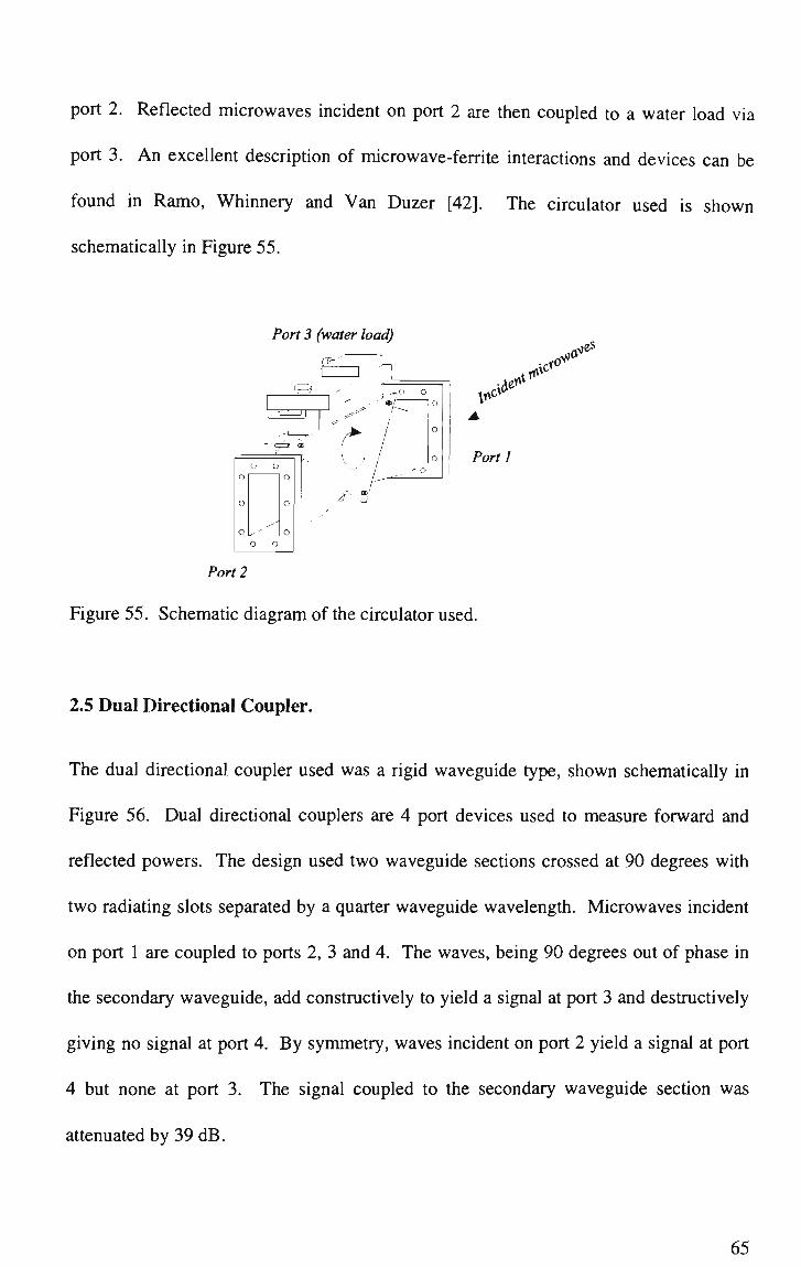
port 2. Reflected microwaves incident on port 2 are then coupled to a water load via
port 3. An excellent description of microwave-ferrite interactions and devices can be
found in Ramo, Whinnery and Van Duzer [42]. The circulator used is shown
schematically in Figure 55.
Port 3 (water load)
•Tr*
o
o
o
u o
^
o o
o
o
n
/
..xrt& r# 1
Port 1
rf-0* .V cf e-
Port2
Figure 55. Schematic diagram of the circulator used.
2.5 Dual Directional Coupler.
The dual directional coupler used was a rigid waveguide type, shown schematically in
Figure 56. Dual directional couplers are 4 port devices used to measure forward and
reflected powers. The design used two waveguide sections crossed at 90 degrees with
two radiating slots separated by a quarter waveguide wavelength. Microwaves incident
on port 1 are coupled to ports 2, 3 and 4. The waves, being 90 degrees out of phase in
the secondary waveguide, add constructively to yield a signal at port 3 and destructively
giving no signal at port 4. By symmetry, waves incident on port 2 yield a signal at port
4 but none at port 3. The signal coupled to the secondary waveguide section was
attenuated by 39 dB.
65

Port 4 Output to Power Meter
It. cv & tv-tr-
;r.T° V i* &
e-
Portl
Port 2
o o 0 1 10
o o
oi-" Io o o
Port 3 Output to Power Meter
Figure 56. Schematic diagram of dual directional coupler used.
2.6 Three Stub Tuner.
A stub tuner is an impedance matching device used to transform the impedance of the
load to match that of the source. If the impedances are matched then maximum power
is transferred to the load since there are no reflections from the load, i.e. the VSWR=1
where VSWR is defined as the voltage standing wave ratio. The method of impedance
matching of a single stub can be used to match any arbitrary, non zero, finite load
impedance to the characteristic impedance of a waveguide [43]. However, the single
stub method requires that the stub be inserted into the waveguide at a specific point,
which varies as the load impedance or the operating frequency is changed. This
requirement often presents practical difficulties since the specified insertion point may
occur at an undesirable location from a mechanical viewpoint or, more importantly, the
impedance of the plasma changes with each operating condition. An alternative method
to single stub impedance matching is to use two or more short circuited stubs inserted
into the waveguide at fixed, though not specific, locations as shown in Figure 57. A
triple or three stub tuner allows a greater range of impedances to be matched than a two
stub tuner. Engineering drawings of the three-stub tuner can be found in Appendix A.
66
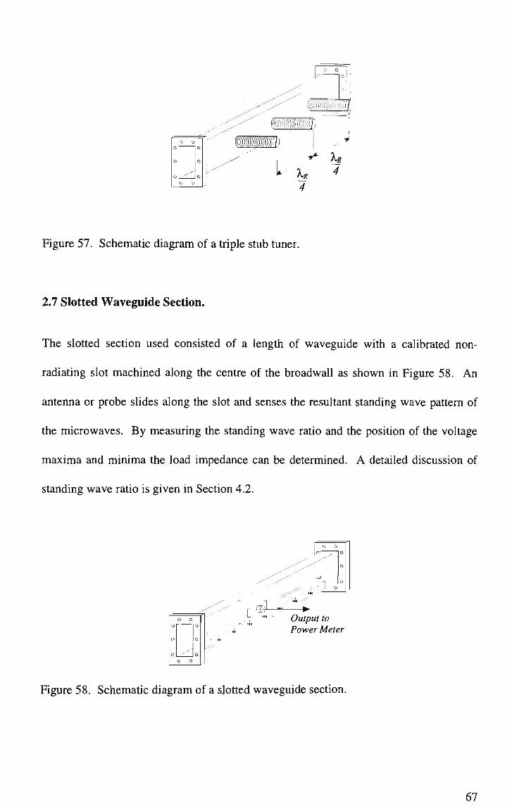
ijjiH!in;(ii':II7J
o o o I ' | o
o o
o I- \ o o o
mi * Xg 4
4
Figure 57. Schematic diagram of a triple stub tuner.
2.7 Slotted Waveguide Section.
The slotted section used consisted of a length of waveguide with a calibrated non-
radiating slot machined along the centre of the broadwall as shown in Figure 58. An
antenna or probe slides along the slot and senses the resultant standing wave pattern of
the microwaves. By measuring the standing wave ratio and the position of the voltage
maxima and minima the load impedance can be determined. A detailed discussion of
standing wave ratio is given in Section 4.2.
CTrr.
o
o
o
o o
0 o
u
0
o
1 - ° i • o
Output to Power Meter
Figure 58. Schematic diagram of a slotted waveguide section.
67

2.8 Power Meter.
Two Hewlett-Packard power meters, models 435A and 435B, with power sensing heads,
model 8481 A, were used for all power measurements. These were calibrated by
Hewlett-Packard during the course of experimentation to ensure accuracy. With 69 dB
attenuation, the power meters were capable of sensing microwave powers between 25 W
and 800 kW FSD though in reality, the attenuators would fail at these power levels. The
maximum power measured by the meters was 6.25 kW.
2.9 Microwave Leakage Meter.
Stray microwave radiation was measured using Holaday Industries, model 1501,
microwave survey meter. This device was calibrated for 2450 MHz and could detect
microwave radiation down to levels of 0.1 mW/cm2. In accordance with the guidelines
for occupational limits, microwave exposure was kept below 2 raW/cm2.
2.10 Welding Table and Controller.
The welding table was constructed in-house and was driven by an RS Components
stepper motor and control electronics via a 1.0 mm pitch lead screw to give a maximum
translation rate of approximately 150 mm/min. The lead screw was later replaced by a
high lead, 47 mm pitch, screw that gave a maximum translation rate of 7.0 m/min. This
replacement was necessary as preliminary welding trials determined that the translation
rate needed to be increased to run with microwave power levels exceeding 2 kW. The
table can be adjusted in three dimensions allowing for the greatest flexibility when it
comes to welding non uniform samples. The workpieces are held in place by a variety
68

of clamping jaws and are butted together in preparation for autogenous welding.
Sample stand-off distance can be varied by 50 mm and table travel is 250 mm. Control
of the table was accomplished via software written in-house using the virtual instrument
application "Visual Designer". A photograph of the welding table can be seen in Figure
59 and engineering drawings in Appendix B.
Figure 59. Photograph of the welding table used.
2.11 Experimental Procedure.
The individual microwave hardware elements are connected as shown in Figure 54.
When attaching microwave waveguide components together, it is necessary to ensure
the flange plates are securely fastened and the waveguides correctly aligned.
Reflections can occur from waveguide discontinuities due to poor alignment and
69

microwave leakage from improperly fastened flange plates, both of which contribute to
unnecessary experimental errors. In general, the slotted waveguide section was only
used during experimentation to determine cavity and/or plasma properties. It was not
used, for example, during welding trials.
When applying microwave power for an experiment, it was necessary to increase the
power slowly. Ramping the microwave power serves to prolong magnetron life. This is
important because a magnetron is an electron tube and therefore, classified as a
consumable by the manufacturer.
2.12 Conclusion.
Equipment able to provide the continuous power levels necessary for practical welding
was not available commercially. However, the equipment detailed in this chapter was
developed to allow for generation, monitoring and detection of microwave radiation
using commercially available and purpose built equipment. Efficient coupling of the
microwave energy to the load is accomplished by insertion of matching elements into
the microwave network. A purpose built welding table and instrumentation as well as
monitoring software and hardware were also constructed to facilitate welding studies.
70
CHAPTER 3. APPLICATOR DEVELOPMENT.
3.1 Introduction.
This chapter deals with applicator design and development. Theoretical considerations,
experimental results and efficiencies for rectangular and as well as cylindrical cavities
are covered. A complete set of cavities with diameters of 60 to 90 mm in increments of
2 mm were constructed to determine the optimum diameter for a cylindrical applicator.
These cavities were then tested at high power and at low power using a network
analyser. Also detailed in the chapter is the development of the waveguide applicator
from the test of concept design to the applicator used for welding trials. Matching with
irises, efficiencies, cooling jacket experiments and materials selection for the waveguide
applicator are also included here. In all instances, microwave power was delivered to
the applicator via WR340 waveguide. This waveguide has internal dimensions of 43 x
86 mm and microwaves propagate within the waveguide in the fundamental or TE10
mode. To generate a plasma, the discharge gas flow rate was set between 2 and 10
litres/minute. Microwave power was then delivered to the cavity and the plasma ignited
by a momentary insertion of an insulated tungsten wire into the ionisation chamber.
3.2 Cylindrical Cavity Design.
The resonant frequency of a cylindrical resonator is determined purely by the radius of
the cylinder. As shown in Chapter 1, the angular frequency is given by;
71

k 2.405
Where (j. and e are the permeability and permittivity of the material contained within the
cavity and a is the radial dimension.
For an air filled cavity resonating at 2450 MHz, the above relation gives a cylindrical
cavity radius of a = 46.8 mm. Note that this dimension only applies for an empty
cavity. With the addition of a ceramic ionisation chamber and plasma, the resonant
radius will change for a fixed driving frequency of 2450 MHz.
To experimentally determine the internal diameter of a cylindrical cavity, containing a
plasma and dielectric load, resonating at 2450 MHz in the TM010 mode, the following
experiment was devised:
a) Firstly, the VSWR and load impedance phase was determined for a set of operating
conditions, e.g. discharge gas flow rate of 5 litres/minute, a microwave power of
1.5 kW and a fixed cavity diameter. (The numerical value of VSWR is the square
root of the ratio of the voltage maxima to voltage minima as measured from the
standing wave pattern of the microwaves in the waveguide. This pattern was
measured using the slotted section and HP power meters given in Section 2.7 and
Section 2.8 respectively).
b) A section of 2.5 mm diameter brass tubing was then cut to such a length as to give
an identical VSWR and load impedance phase when examining the S21 parameters
72

on a network analyser. The S21 parameter is the ratio of the amplitude of the wave
leaving port 2 to the wave entering port 1. The rationale for using the brass tube to
mimic the plasma is based on the fact that the plasma behaves as a partially
conducting medium since it has some degree of ionisation. This is well illustrated
by examining the standing wave pattern for the waveguide applicator shown in
Figure 60. Extrapolating either curve to zero on the standing wave scale gives a
near minimum in the electric field strength, which is consistent with the boundary
conditions of E=0 on a conductor.
c) The length of brass tubing was then inserted into the ionisation chamber of a cavity
modelled from polystyrene and aluminium tape to simulate the plasma. Ideally,
when examined on the network analyser the resonant frequency of the cavity with
the dielectric and the simulated plasma would be 2450 MHz. If this was not the
case, a new cavity with a different inside diameter, hopefully giving the desired
resonant frequency, could be quickly constructed. This method of rapid
prototyping was relatively easy to do using polystyrene models wrapped in
aluminium tape. A photograph of a selection of polystyrene models can be seen in
Figure 61.
73

1000
a "3 800
g1 600
GO
2 400 4?
200
0 •1
• •
1P 1
• • •
1
JP J1 • •
I •_
1
1
1 1
••
1 »• ••
•
f£
I !
• i
•
•
•
•
•
- f " 1
Sliding short at -78 m m , Load at zero on ruler
ztzztzzt -1- - j - 1 1 1 -M 1
• • • T ; ; ; ! i !
•
• ; !
•
• •
1 1 '
. •
; .
• • •
i
I ' i
|
-4-— i
-80 -60 -40 -20 0 20 40 60 80 100 120 140 160 180 200 220 240 260 280
Standing Wave Scale (mm)
Figure 60. Standing wave pattern about the ionisation chamber for a waveguide
applicator. Forward CW microwave power = 360 W. Note: Graph in region -80 to 0
scaled down by a factor of 10.
Figure 61. Rapid prototyping polystyrene models used to model plasma/cavity system.
74
The network analyser used, a Hewlett-Packard model 8753C with model 85046A S
parameter test set, is designed for low power applications and so could not simulate the
change in effective dielectric constant of the applicator system with the change in
temperature associated with high power operation. As such, it was not known if each of
the polystyrene models would be capable of initiating and sustaining a plasma.
Therefore, a new experiment was devised to accommodate the elevated temperatures of
the applicator system when operating at high powers.
The four steps in the new experiment were:
a) Two cylindrical applicators were constructed from aluminium bar with outside
diameters of 100 mm and internal diameters of 50 and 60 mm. The first was 60 mm
long and the second 100 mm. The 100 mm long cavity is shown photographically in
Figure 62.
b) These applicators were then used to generate high power plasmas. Quartz and then
boron nitride were used as the ionisation chambers whilst using argon and then
nitrogen as the discharge gas.
c) The resonant frequency of the applicator was then determined using the network
analyser under three different conditions; empty, with ionisation chamber and with
ionisation chamber and simulated plasma.
d) The inside diameter of the applicator was then increased by 2 mm and the process of
high power and network analyser tests repeated. This was repeated until the I.D.'s
of the 60 and 100 mm long cavities reached 76 and 92 mm respectively. The work
on the 60 mm long cavity was performed by Duarte DoRego, a research student
from the Department of Mechanical Engineering at the University of Wollongong,
and is included here for completeness.
75

Figure 62. Photograph of 100 m m long cylindrical cavity.
Figure 63 shows the resonance characteristics of the 100 mm cylindrical cavity as a
function of internal diameter for the following conditions: empty, loaded with boron
nitride dielectric and loaded with boron nitride dielectric and simulated plasma. Also
represented for interest on the graph is the theoretical frequency for an empty cavity
resonating in the TM010 mode. Quite clearly, the theoretical values bear no
resemblance to the experimentally measured values. The main reason for this may be an
inappropriate coupling mechanism between the waveguide and the cavity. Since the
mode excited within a cylindrical cavity is critically dependent on the coupling
mechanism, one needs to carefully choose the coupling method to generate the required
field pattern. Instead of using a rectangular to cylindrical waveguide transition, an
inductive loop could have been used to couple energy to the cavity. This may have
produced the correct field pattern but would necessitate the use of coaxial cable to
76
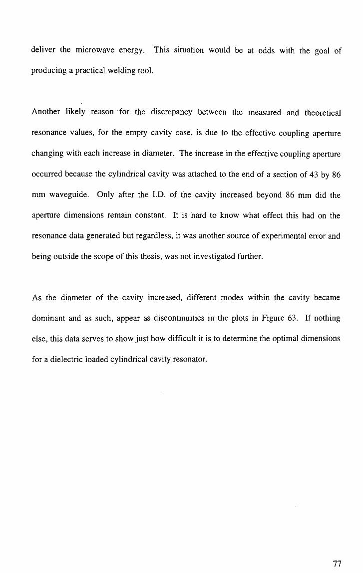
deliver the microwave energy. This situation would be at odds with the goal of
producing a practical welding tool.
Another likely reason for the discrepancy between the measured and theoretical
resonance values, for the empty cavity case, is due to the effective coupling aperture
changing with each increase in diameter. The increase in the effective coupling aperture
occurred because the cylindrical cavity was attached to the end of a section of 43 by 86
mm waveguide. Only after the I.D. of the cavity increased beyond 86 mm did the
aperture dimensions remain constant. It is hard to know what effect this had on the
resonance data generated but regardless, it was another source of experimental error and
being outside the scope of this thesis, was not investigated further.
As the diameter of the cavity increased, different modes within the cavity became
dominant and as such, appear as discontinuities in the plots in Figure 63. If nothing
else, this data serves to show just how difficult it is to determine the optimal dimensions
for a dielectric loaded cylindrical cavity resonator.
77

I 2200 o g OS 2000
1800
' Empty Cavity
Cavity + B N
Cavity + B N + Brass
Theoretical Freq.
60 64 68 72 76 80 84 Cavity Internal Diameter (mm)
88 92
Figure 63. Resonance characteristics as a function of cavity diameter for the 100 m m
long cavity.
Table 7 contains the cavity diameter/plasma data for both the 60 m m and 100 m m long
cavities. This data was generated using CW microwave power up to 2 kW with a triple
stub tuner used to match the load presented by the plasma/cavity system to the source.
The boron nitride used for the ionisation chamber was not pure and so has a higher loss
factor than the pure material. The greater the loss factor of a material, the more readily
it will absorb microwave energy. For example, distilled water has a loss factor of 76.7
[44], pure boron nitride has a loss factor of 0.00075 and quartz 0.0002 at 3000MHz.
This higher loss factor meant the tube heated through the absorption of microwave
energy and provided an electron source for plasma initiation (Figure 64 shows a
photograph of an impure boron nitride ionisation chamber that has failed due to
oxidation). The quartz tube was essentially transparent to microwaves and could not
initiate a plasma since it did not heat up. This is verified by experimental results given
78

in Table 7. The fact that a plasma could not be initiated in the quartz ionisation
chamber suggests that a plasma cannot be initiated purely from dielectric breakdown of
the discharge gas but needs initiating through some secondary mechanism such as
thermionic emission of electrons from the heated ionisation chamber, or from the spark
generated on the tip of a tungsten wire inserted into the cavity. This point is important
since it was initially thought that it might be possible to design an applicator that would
spontaneously initiate a plasma. From Table 7, it is also evident that it is easier to
generate an argon plasma than a plasma from nitrogen gas. This is consistent with the
ionisation energy of argon being lower than for nitrogen gas. However, the situation is
complicated since nitrogen gas is a diatomic molecule that can absorb energy in both
vibrational and rotational modes.
There was no attempt to determine the heat capacity or temperature of the plasma during
these experiments so it is not clear which internal diameter allowed the cavity to
resonate at 2450 MHz, thereby providing the "hottest" plasma. The fact that the plasma
could be easily generated for diameters of 88 and 78 mm, with nitrogen and argon as the
discharge gas respectively, implies that the plasmas generated from these two gases have
different properties and so behave differently.
79

Figure 64. Photograph showing oxidised boron nitride ionisation chamber
As it happens, the I.D. of the cavity is only critical if there are no matching elements in
the microwave network since a reasonable match for most I.D.'s was obtained by using
a stub tuner arrangement. The maximum efficiency obtained for a cylindrical cavity
was about 60% where the efficiency is defined as:
r,nn. . Forward Power - Reflected Power Efficiency =
Forward Power
It should be noted that there was no mechanism for fine tuning the resonant frequency
of these cavities and this may well be the reason for the relatively low efficiency
recorded.
80

Cavity
I.D.
50
52
54
56
58
60
62
64
66
68
70
72
74
76
78
80
82
84
86
88
90
92
60 M M CAVITY
BN
N2
N
N
N
N
Y
-
Y
N
Y
-
N
-
Y
Y4
BN
Ar
N
N
N
Y1
Y2
-
Y
Y
Y
N
N
N
Y3
Y
Si02
N2
N
N
-
-
N
-
-
-
-
-
-
-
N
-
Si02
Ar
N
N
N
N
N
-
-
N
-
N
N
N
N
N
100 M M CAVITY
BN
N2
N
Y
N
Y
N
Y
N
N
Y
Y
Y
Y
Y
N
Y6
Y
N
BN
Ar
N
Y
Y
Y
Y
Y
Y
Y
Y
Y5
Y
Y
Y
Y
Y
Y
Y
Si02
N2
-
-
-
-
N
-
-
-
N
-
-
-
-
-
N
N
-
Si02
Ar
-
-
-
-
N
-
-
N
N
N
N
N
N
N
N
-
-
81

Notes: All dimensions in m m
Y
N
1.
2.
3.
4.
5.
6.
-
: plasma was generated
: no plasma was generated
Degraded B N tube
Plasma generation intermittent
Feeble plasma
Degraded B N tube
Plasma easily generated, B N not glowing red hot
B N not glowing red hot
Data not taken
Table 7. Cylindrical cavity internal diameter/plasma data.
3.3 Rectangular Cavity Design.
A rectangular cavity with dimensions of 43x45x45 mm was constructed from
aluminium and had two fine tuning stubs. The first stub was aligned parallel with the
broadwall of the attached waveguide and was positioned mid wall. The second was
aligned parallel with the short-wall of the attached waveguide as shown in Figure 65.
This cavity is similar in design to that of Matusiewicz [34] in as much as the cavity is
attached to a section of standard waveguide and has smaller dimensions than that of the
waveguide. However, the method of tuning is different as an inductive iris is not used
in the design detailed here.
82
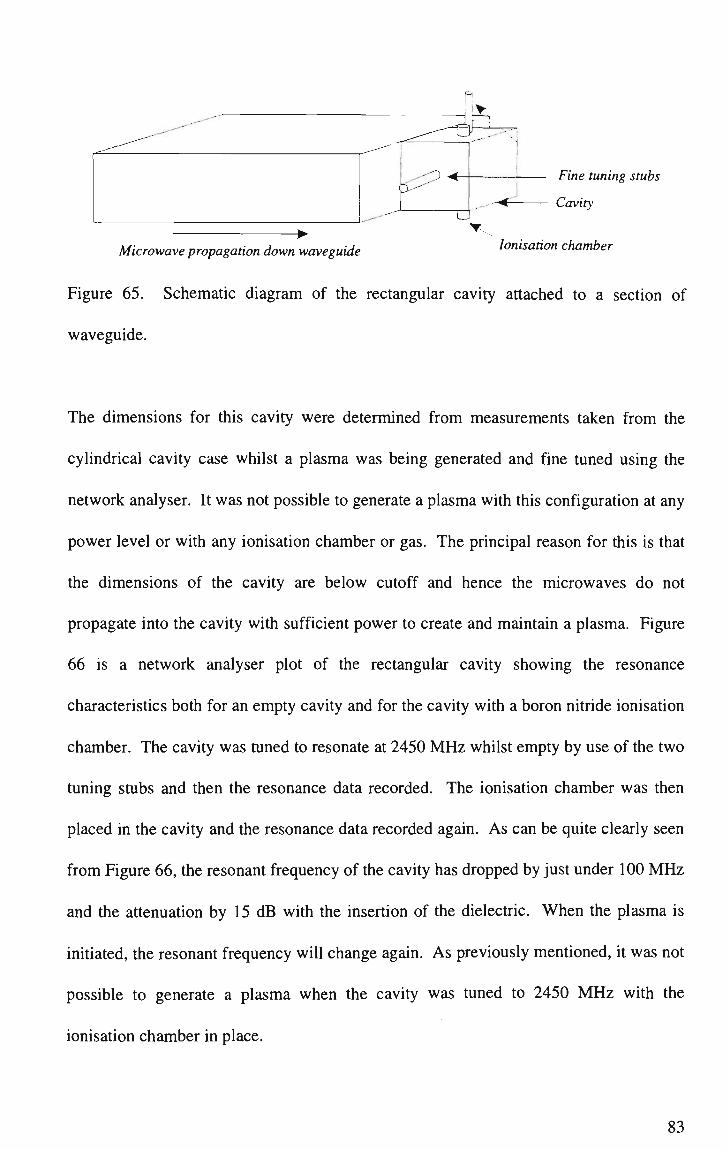
F1
=£ Fine? tuning stubs
----< Cavity
Microwave propagation down waveguide Ionisation chamber
Figure 65. Schematic diagram of the rectangular cavity attached to a section of
waveguide.
The dimensions for this cavity were determined from measurements taken from the
cylindrical cavity case whilst a plasma was being generated and fine tuned using the
network analyser. It was not possible to generate a plasma with this configuration at any
power level or with any ionisation chamber or gas. The principal reason for this is that
the dimensions of the cavity are below cutoff and hence the microwaves do not
propagate into the cavity with sufficient power to create and maintain a plasma. Figure
66 is a network analyser plot of the rectangular cavity showing the resonance
characteristics both for an empty cavity and for the cavity with a boron nitride ionisation
chamber. The cavity was tuned to resonate at 2450 MHz whilst empty by use of the two
tuning stubs and then the resonance data recorded. The ionisation chamber was then
placed in the cavity and the resonance data recorded again. As can be quite clearly seen
from Figure 66, the resonant frequency of the cavity has dropped by just under 100 MHz
and the attenuation by 15 dB with the insertion of the dielectric. When the plasma is
initiated, the resonant frequency will change again. As previously mentioned, it was not
possible to generate a plasma when the cavity was tuned to 2450 MHz with the
ionisation chamber in place.
83

CHI S21 log MAG 10 dB/ REF 0 dB 1: -27.843 dB
2 450.174 004 MHz
M A R 1 C E R 1 (Cavity plus Ionisation (bhamber) ; 2: -12.552 dB
2 368.774 004 MHz 2.450174004 G H z
M A R K E R 2 (Empty Cavity) 2.368774004 GFIz
;r J*
,.--
CENTRE 2 450.000 000 MHz SPAN 1 100.000 000MHz
Figure 66. Resonance characteristics of the rectangular applicator. N.B. ;t-axis units are
Frequency (100 MHz/division) and y-axis units are Attenuation (10 dB/division).
3.4 Waveguide Cavity Design.
A schematic diagram of the rectangular waveguide applicator is given in Figure 67. As
can be seen from the diagram, the applicator is a section of waveguide fitted with a
sliding short circuit, or movable tuning plunger, with the ionisation chamber passing
centrally through the broadwall of the waveguide.
Plasma Gas
Ionisation A Jntident Chamber Microwaves
o f
Plasma Beam Figure 67. Schematic diagram of the W R 3 4 0 waveguide applicator
84
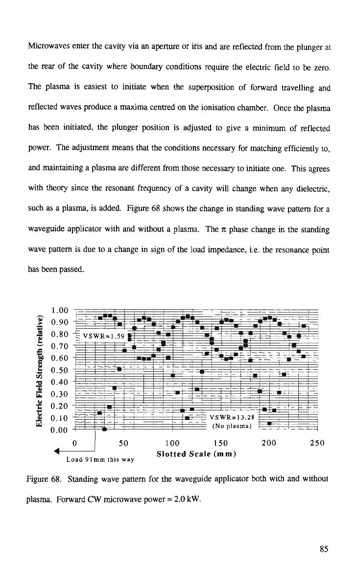
Microwaves enter the cavity via an aperture or iris and are reflected from the plunger at
the rear of the cavity where boundary conditions require the electric field to be zero.
The plasma is easiest to initiate when the superposition of forward travelling and
reflected waves produce a maxima centred on the ionisation chamber. Once the plasma
has been initiated, the plunger position is adjusted to give a minimum of reflected
power. The adjustment means that the conditions necessary for matching efficiently to,
and maintaining a plasma are different from those necessary to initiate one. This agrees
with theory since the resonant frequency of a cavity will change when any dielectric,
such as a plasma, is added. Figure 68 shows the change in standing wave pattern for a
waveguide applicator with and without a plasma. The n phase change in the standing
wave pattern is due to a change in sign of the load impedance, i.e. the resonance point
has been passed.
1.00 cu
% 0.80 -VSWR=1.59
B
• * _ •
-a
E u "C • _ -
3
Load 91mm this way
100 150 Slotted Scale ( m m )
250
Figure 68. Standing wave pattern for the waveguide applicator both with and without
plasma. Forward CW microwave power = 2.0 kW.
85
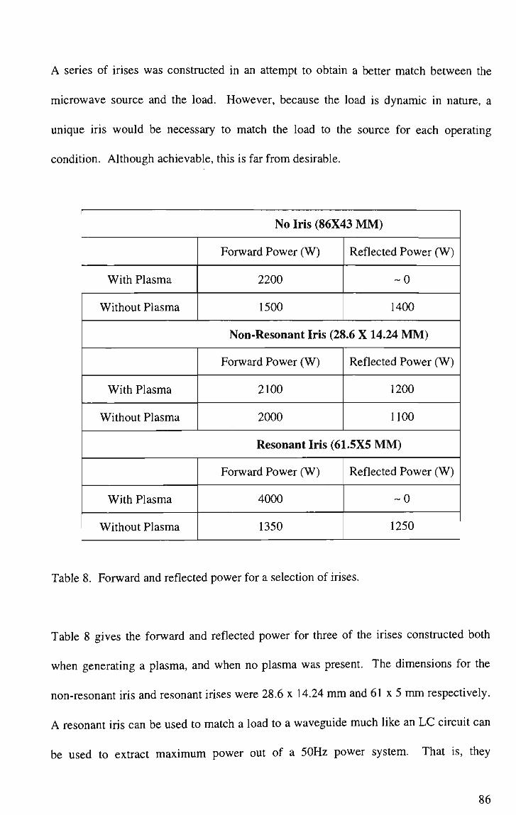
A series of irises was constructed in an attempt to obtain a better match between the
microwave source and the load. However, because the load is dynamic in nature, a
unique iris would be necessary to match the load to the source for each operating
condition. Although achievable, this is far from desirable.
No Iris (86X43 M M )
With Plasma
Without Plasma
Forward Power (W)
2200
1500
Reflected Power (W)
~0
1400
Non-Resonant Iris (28.6 X 14.24 M M )
With Plasma
Without Plasma
Forward Power (W)
2100
2000
Reflected Power (W)
1200
1100
Resonant Iris (61.5X5 M M )
With Plasma
Without Plasma
Forward Power (W)
4000
1350
Reflected Power (W)
~0
1250
Table 8. Forward and reflected power for a selection of irises.
Table 8 gives the forward and reflected power for three of the irises constructed both
when generating a plasma, and when no plasma was present. The dimensions for the
non-resonant iris and resonant irises were 28.6 x 14.24 mm and 61 x 5 mm respectively.
A resonant iris can be used to match a load to a waveguide much like an LC circuit can
be used to extract maximum power out of a 50Hz power system. That is, they
86
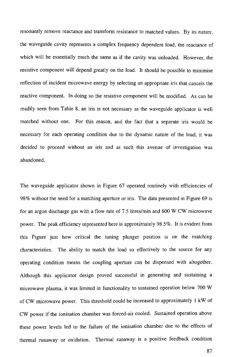
resonantly remove reactance and transform resistance to matched values. By its nature,
the waveguide cavity represents a complex frequency dependent load, the reactance of
which will be essentially much the same as if the cavity was unloaded. However, the
resistive component will depend greatly on the load. It should be possible to minimise
reflection of incident microwave energy by selecting an appropriate iris that cancels the
reactive component. In doing so the resistive component will be modified. As can be
readily seen from Table 8, an iris is not necessary as the waveguide applicator is well
matched without one. For this reason, and the fact that a separate iris would be
necessary for each operating condition due to the dynamic nature of the load, it was
decided to proceed without an iris and as such this avenue of investigation was
abandoned.
The waveguide applicator shown in Figure 67 operated routinely with efficiencies of
98% without the need for a matching aperture or iris. The data presented in Figure 69 is
for an argon discharge gas with a flow rate of 7.5 litres/min and 600 W CW microwave
power. The peak efficiency represented here is approximately 98.5%. It is evident from
this Figure just how critical the tuning plunger position is on the matching
characteristics. The ability to match the load so effectively to the source for any
operating condition means the coupling aperture can be dispensed with altogether.
Although this applicator design proved successful in generating and sustaining a
microwave plasma, it was limited in functionality to sustained operation below 700 W
of CW microwave power. This threshold could be increased to approximately 1 kW of
CW power if the ionisation chamber was forced-air cooled. Sustained operation above
these power levels led to the failure of the ionisation chamber due to the effects of
thermal runaway or oxidation. Thermal runaway is a positive feedback condition
87

whereby the ability of the ceramic ionisation chamber to absorb microwave energy
increases with temperature. As the ionisation chamber heats due to contact with the
plasma, it becomes more electrically conducting and absorbs more microwave energy,
which increases the temperature of the tube even further. The result is that the
ionisation chamber eventually heats until the melting point is reached and then fails.
80
70
12 60
as 50
40
£30
20
10
y <
ll I
* % Power Reflectec
•VSWR
• 4
• | • 1
r
* 1
<
' • . " 1
I
- 1 »
•
1 ! )
W !
+ :
:
' 1 1
• •
1 1
' i 1 i •
|
~ T 1 * , !
17
15
r 13
n
CO
75 76 77 78 79 80 81 Sliding Short-Load Distance (mm)
82 83
Figure 69. Percentage reflected power and V S W R as a function of sliding short
position.
3.5 Water-Cooled Waveguide Cavity Design.
To overcome the problem of thermal runaway, a more efficient mechanism for heat
removal was required. The opportunity arose [45] to discuss the cooling methods of
Arata et al [16] with Professor Shoji Miyake from the Japanese Welding Research
Institute. Though the cooling methods employed in the research of Arata were for
determining the heat loss through the walls of the ionisation chamber, using calorimetric
methods, it was reasoned that a similar method could be used to remove the heat from
88

the ionisation chamber thereby preventing thermal runaway. It was uncertain whether
such a manner could be employed since the applicator design and more importantly, the
ionisation chamber I.D., were different from those of Arata. As mentioned in Section
1.3, a helical gas flow in the ionisation chamber (10 mm I.D.) of Arata produced a cold
gas wall that prevented the plasma from coming into contact with the ionisation
chamber. As the ultimate goal of this research was to produce an applicator capable of
welding sheet steel, the 10 mm I.D. ionisation chamber of Arata would be far from
desirable. In addition, it would be extremely unlikely that one could create a helical
flow of gas inside a ionisation chamber with an I.D. of only 1-3 mm and so produce
the cold gas wall.
Plasma Gas
Coolant In 1 I
m_in Ionisation < incident Chamber Microwaves
1-0
l -* Coolant Out Plasma Beam
Figure 70. Water cooled waveguide applicator.
The waveguide applicator was modified to determine whether it was possible to initiate
and sustain a plasma inside an annulus of water. The modifications are reflected in
Figure 70 (compare Figure 67). For the initial experiment CW microwave power was
varied between 0.3 and 1.6 kW and the argon discharge gas flow rate set at 7.5 l/min.
Pyrex was used for the ionisation chamber and had dimensions of 3.44 x 5.10 mm (I.D.
89
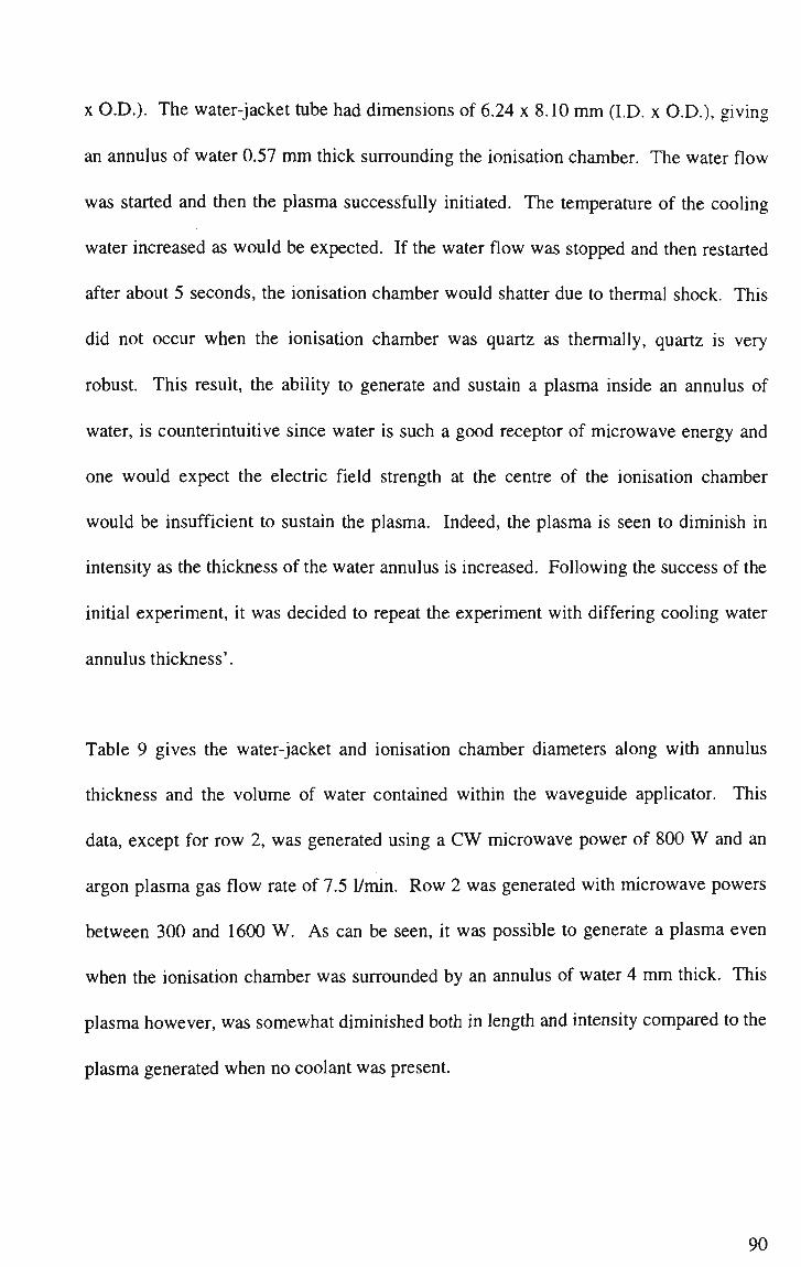
x O.D.). The water-jacket tube had dimensions of 6.24 x 8.10 m m (I.D. x O.D.), giving
an annulus of water 0.57 mm thick surrounding the ionisation chamber. The water flow
was started and then the plasma successfully initiated. The temperature of the cooling
water increased as would be expected. If the water flow was stopped and then restarted
after about 5 seconds, the ionisation chamber would shatter due to thermal shock. This
did not occur when the ionisation chamber was quartz as thermally, quartz is very
robust. This result, the ability to generate and sustain a plasma inside an annulus of
water, is counterintuitive since water is such a good receptor of microwave energy and
one would expect the electric field strength at the centre of the ionisation chamber
would be insufficient to sustain the plasma. Indeed, the plasma is seen to diminish in
intensity as the thickness of the water annulus is increased. Following the success of the
initial experiment, it was decided to repeat the experiment with differing cooling water
annulus thickness'.
Table 9 gives the water-jacket and ionisation chamber diameters along with annulus
thickness and the volume of water contained within the waveguide applicator. This
data, except for row 2, was generated using a CW microwave power of 800 W and an
argon plasma gas flow rate of 7.5 l/min. Row 2 was generated with microwave powers
between 300 and 1600 W. As can be seen, it was possible to generate a plasma even
when the ionisation chamber was surrounded by an annulus of water 4 mm thick. This
plasma however, was somewhat diminished both in length and intensity compared to the
plasma generated when no coolant was present.
90

Ionisation Chamber
(ID.)
10.3
3.44
8.04
5.80
5.76
4.00
3.21
(O.D.)
12.48
5.10
10.06
9.00
8.00
6.10
5.04
Water Jacket
(LD.)
13.26
6.24
13.26
13.26
13.26
13.26
13.26
(O.D.)
16.10
8.10
16.10
16.10
16.10
16.10
16.10
Annulus
Thickness
0.39
0.57
1.60
2.13
2.63
3.58
4.11
Water Vol.
(mm3)
678.05
436.59
2520.22
3203.56
3776.66
4681.42
5080.22
Plasma
Generation
Yes2
Yes
Yes2
Yes2
Yes2
Yes1 2
Yes1 2
Notes: All dimensions in millimetres.
1. Plasma somewhat diminished in intensity.
2. Microwave power 800 W .
Table 9. Experimental water-jacket thickness data.
The final design of the water cooled waveguide applicator was drawn from many
elements of the experimental programme, not the least the success of the water cooled
ionisation chamber, and needed to take into account the operational requirements
necessary for welding sheet steel. The design, as given in Figure 71, employs a counter
current coolant flow in which the coolant flows past the hottest part of the ionisation
chamber first. The coolant enters through the bottom of the waveguide and travels
along a small diameter brass tube before reaching the void between the coolant jacket
and the outside of the ionisation chamber near the plasma exit orifice. The coolant then
travels along the ionisation chamber and exits through a quick-fit connector at the top of
the applicator. The other advantage of counter current cooling is that the water-jacket
91

fills from the bottom up, thereby minimising possible air voids. This is especially
important if the annulus thickness, the distance between the O.D. of the ionisation
chamber and the I.D. of the coolant or water-jacket, is small. The coolant is contained
by Viton O-ring seals between the outside of the quartz coolant jacket and the applicator
body. The coolant is prevented from leaking into the plasma region by a taper lock fit
between the ends of the ionisation chamber and the applicator body. A compressive
force is applied to the taper lock by an adjustable brass face-plate at the plasma exit
orifice.
Compression Spring
Screw -In Constricting Baffle
Ionisation Chamber
Sliding Short Circuit Plunger
Coolant In
[j Plasma Initiation Plunger
Discharge Gas In
Coolant Out
Viton O-Ring Seals
Coolant Jacket
Taper Lock Fit
Brass Face-Plate Y Plasma Beam
Figure 71. Final design of the water cooled waveguide applicator.
The discharge gas enters the applicator through a quick-fit connector and then passes
through a constricting baffle before entering the ionisation chamber to be ionised and
ejected as a plasma. The purpose of the constricting baffle is twofold. Firstly, the gas
feed hole can be angled and offset to optimise gas flow dynamics within the ionisation
chamber. And secondly, the small diameter gas feed hole ensures that the plasma only
92

flows out through the exit orifice and not back along the gas feed line. The plasma is
initiated by a momentary insertion of the spring loaded initiating plunger into the
waveguide. No microwave leakage occurs during this action because the plunger is in
intimate contact with the applicator body which is at earth potential.
The ionisation chamber in the ultimate design was fashioned from pure boron nitride
and had an I.D. and O.D. of 3 mm and 15 mm respectively. The coolant jacket was
fashioned from quartz and had an I.D. and O.D. of 16 mm and 19 mm respectively.
This gave an annulus thickness of 0.5 mm which was more than adequate for a 6 kW
plasma when coolant flow rates were of the order of 0.5 litres/minute. An attempt to use
alumina for the ionisation chamber in this design was abandoned because the tube
would shatter due to thermal shock whenever the plasma was initiated. Figure 72 and
Figure 73 show the dismantled applicator with elements of the cooling system.
Specifically, in Figure 72 the alumina ionisation chamber and cooling jacket are visible
as are the coolant feed, gas manifold and associated brass componentry. Figure 73
shows the general arrangement of the applicator without the top plate, ionisation
chamber and gas feed system. The tuning plunger is clearly visible, as is the water feed
line and microwave transparent window. The applicator sits atop an atmospheric
control vessel of I.D. 400 mm. This vessel houses the welding table and allows welding
in a controlled atmosphere or at reduced pressure. It also has a viewing window to
monitor welding progress.
93
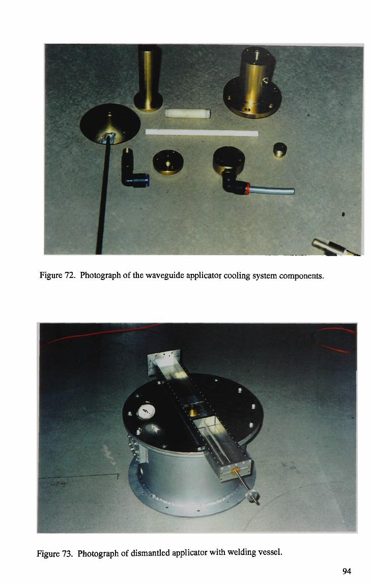
Figure 72. Photograph of the waveguide applicator cooling system components.
Figure 73. Photograph of dismantled applicator with welding vessel.
94
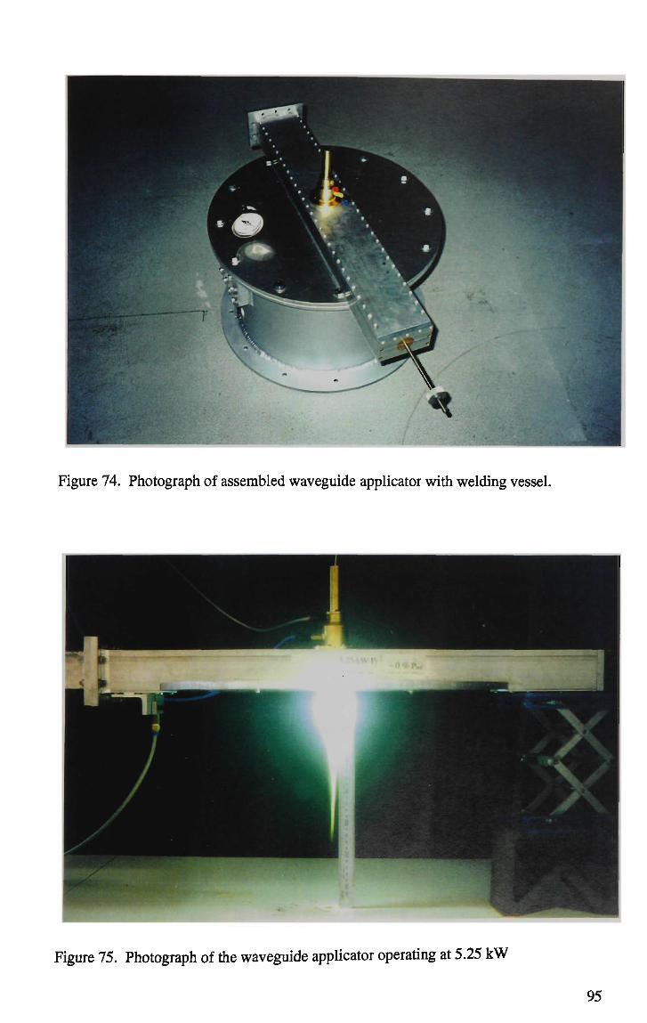
Figure 74. Photograph of assembled waveguide applicator with welding vessel.
Figure 75. Photograph of the waveguide applicator operating at 5.25 k W
95

Close-up detail of the assembled applicator without the welding vessel can be seen in
Figure 75. This photograph shows the applicator generating a 5.25 kW plasma beam
with an argon discharge gas flow rate of approximately 5 litres per minute. As can be
seen from this photograph, the plasma beam is well collimated over a length in excess of
220 mm.
The efficiency of the water-cooled waveguide applicator was no different from that of
the non cooled version. For example, it was possible to adjust the reflected power down
to 10 W with a forward microwave power of 3 kW. This gives an efficiency in excess
of 99.5 %. It should be noted however that this efficiency does not take into account
losses to the walls.
3.6 Conclusion.
Attempts at producing a cylindrical resonant cavity applicator suitable for materials
welding and joining applications were unsuccessful. The use of rapid prototyping, a
network analyser and high power tests showed that the maximum efficiency attainable
for the investigated cavity design was only 60 %. Rapid prototyping of the cavity
involved sculpting the desired cavity from Polystyrene foam and then wrapping it in
conducting aluminium tape. When examined using the network analyser, these
prototypes behaved as machined aluminium cavities would but take a fraction of the
time to construct. Being made from foam however, meant that operation was limited to
low power tests only. The low power limitation meant that it was not possible to use the
network analyser to model the cavity whilst generating a plasma. To overcome this, a
method was developed whereby a small diameter brass tube was used to simulate the
96
plasma for the low power tests. The dimensions of the brass tube were selected such
that it gave the same VSWR and load phase impedance when examined on the network
analyser. Rapid prototyping of the cavity as well as simulation of the plasma by a brass
insert allowed the electrical properties of the cavity to be determined at low powers.
High power tests were performed on a 100 mm long cavity fashioned from aluminium.
The internal diameter of the cavity started at 60 mm and was increased in 2 mm steps
until it reached 92 mm. For each of these increments a high power test was performed.
Results of these measurements showed that it was possible to generate a plasma for each
I.D. when using argon as the discharge gas. Results also showed that it was not possible
to spontaneously generate a plasma in argon using a cylindrical cavity. The electric
field strength of the microwaves in the cavity is insufficient to cause dielectric
breakdown in argon and thus, a secondary mechanism is necessary to initiate the
plasma. In the case of pulsed power and an impure boron nitride ionisation chamber,
this mechanism was thermionic emission of electrons from the heated tube. For the case
of CW microwave power and either quartz or pure boron nitride as the ionisation
chamber, it was necessary to insert a length of tungsten wire into the ionisation chamber
to initiate the plasma.
It was also not possible to generate a plasma in a rectangular cavity with dimensions 45
x 45 x 43 mm because the dimensions are below cut-off and thus, insufficient
microwave energy penetrates the cavity to sustain a plasma. Previous attempts by
researchers at producing high power plasmas in cavities with small diameter ionisation
chambers have resulted in failure due to materials limitations. In effect, the ionisation
chambers have melted due to thermal runaway. However, the task of designing,
97

building and testing a microwave plasma applicator that is suitable for welding and
joining applications has been successfully completed using a waveguide applicator. The
applicator is efficient, stable, operates at high powers and produces a highly collimated
plasma beam and is shown operating at 5.25 kW in Figure 75. Routine efficiencies are
greater than 98% without the use of a coupling aperture or iris and extended operation at
microwave power levels of 6 kW is possible.
Previous to the development of this device, power levels for comparable applicators
were limited to sustained operation below about 1 kW. The design detailed here is
revolutionary in that it uses a small diameter, water cooled ionisation tube to produce a
high power collimated beam. As shown in Table 6, a systematic investigation of these
operating parameters is all but absent from the literature. Indeed, this is the first time
that a high power plasma generated in a small diameter ionisation chamber has been
demonstrated.
98
CHAPTER 4. CHARACTERISATION OF THE PLASMA/APPLICATOR
SYSTEM.
4.1 Introduction.
Welding has been an accepted method for joining disparate samples for many years with
welding techniques and parameters being optimised through trial and error methods. In
essence, welding is still classified as a black art since many processes are not well
understood. As the use of a microwave induced plasma beam as a welding tool is
absent from the literature, much work at characterising the beams properties as a
function of external parameters is necessary. This chapter deals with the
characterisation of the plasma/applicator system. Specifically, the way the applicator
responds to external variables such as power, gas flow rate, applicator tuning etc. is
characterised as this information is essential to produce a device capable of consistent,
high quality welding. To that end, the research covered can be broadly divided into two
sections. The first deals with the electrical properties of the plasma and the second with
determination of the physical parameters of the plasma such as length, pressure and
temperature. The purpose of the applicator is to produce a well-collimated beam of
plasma into which is deposited as much microwave power as possible to produce a
practical welding tool. The amount of power deposited in the plasma is a measure of
the efficiency of the applicator and can be determined by measuring the VSWR of the
system. This means it is necessary to have a thorough understanding or knowledge of
what governs, controls and characterises the VSWR so that the applicator can be
operated at maximum efficiency.
99

Section 4.2 deals with the background theory of V S W R and how it relates to the
microwave power travelling within the waveguide. Section 4.3 examines the VSWR of
the non-cooled waveguide applicator, described in Section 3.4, as a function of the
variables determining the operating characteristics of the plasma. It specifically covers
microwave power, discharge gas flow rate and the state of tuning of the system. VSWR
measurements on the slotted line also allow the plasma impedance to be determined,
from which a simple electrical circuit model of the plasma/applicator system is
developed, given in Section 4.4. Section 4.5 examines the real and imaginary
impedance of the plasma as a function of the same variables that determine the
operating characteristics of the plasma listed above.
Section 4.6 and 4.7 investigates the VSWR and impedance attributes of the plasma
beam, respectively, as produced by the water-cooled applicator. The impedance
attributes of the water-cooled and non-cooled plasma beam are compared to those
reported in the literature in Section 4.8. The plasma beam length as a function of
microwave power and discharge gas flow rate is shown photographically in Section 4.9.
To overcome materials limitations associated with the limited operating range of
thermocouples, two methods of indirect temperature determination were devised and are
given in Section 4.10. These methods examined the heat capacity of the plasma as well
as the relative plasma temperature using heat conduction phenomena and K-type
thermocouples. Lastly, a differential pressure transducer was used to measure the
pressure exerted by the plasma beam for the various operating parameters. These results
are reported in Section 4.11.
100

4.2 Background Theory of V S W R .
When microwaves are incident on a waveguide discontinuity, part or all the microwave
energy is reflected and a standing wave envelope or pattern is formed [46]. Figure 76
shows the standing wave pattern for the case where the reflected and incident waves
have identical amplitudes. The distance separating successive voltage standing wave
maxima or minima is half of the waveguide wavelength in the slotted section, X .
•8 mtm
•a
i o
Z 2
3
l --
A A A A : :
o*-0
Discontinuity
• •
A s g — > 2
• \
10
Distance Along Waveguide
Figure 76. Schematic representation of a V S W R pattern.
The Electric field and hence the voltage along a waveguide is of the form
:=£,sin(ff) or V=V0sin(^)
The maximum value of the standing wave envelope corresponds to the sum of the
amplitudes of the incident and reflected waves, whilst the minimum corresponds to the
difference between the two. By sampling the microwave power along the slotted
101

section, the position of the voltage maxima and minima in relation to the load distance
can be determined. The VSWR is then given as
VSWR = ^-min
The ratio of the reflected wave to the incident wave is defined as the reflection
coefficient, p. In terms of the VSWR, the magnitude of the reflection coefficient is
given by
VSWR-l P~VSWR + l
In general, the standing wave envelope is not a sine curve, the minimum being sharper
than the maximum [47]. However, in the limiting case of p=l the curve does have the
form of a rectified sine function. Also, as the condition p=0 is approached, the curve
approximates a sinusoidal variation.
4.3 VSWR Measurements on the Non-Cooled Waveguide Applicator.
This section presents data obtained using the non-cooled waveguide applicator with CW
microwave radiation and argon as the discharge gas. The experimental set-up is shown
schematically in Figure 77. The data used to determine the VSWR was gathered using
the following procedure:
a) The plasma was initiated and the microwave power adjusted to the desired level.
102

b) The tuning plunger and then the tuning stubs adjusted to give a minimum reflected
power.
c) The probe was inserted into the slotted section as close as possible to the load and
the resultant power measured. *-
d) The power level at the probe and the probe position recorded. The power recorded
is the resultant power from superposition of forward and reflected microwaves
within the waveguide. It is not the power as set in step a), which is the total forward
power.
e) The probe was then repositioned in slotted section 5 m m further away from the load
(ionisation chamber).
f) The power level and the probe position was recorded again.
g) The process of repositioning and measuring the power level was repeated for the full
length of slotted section, approximately 200 m m .
Slotted Section
&
Magnetron Circulator Directional Coupler Waveguide Applicator
Figure 77. Schematic diagram of experimental apparatus.
This data, when plotted as the square root of the power as a function of slotted section
reading (or standing wave scale), typically gives results as shown in Figure 78. The data
labelled by V S W R = 1 . 3 is typical of the V S W R curve for the case where the source and
load are mismatched. The VSWR=1.1 curve may indicate the presence of higher order
modes generated at the load. These higher modes are cut off and are therefore
103
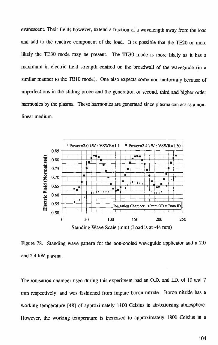
evanescent. Their fields however, extend a fraction of a wavelength away from the load
and add to the reactive component of the load. It is possible that the TE20 or more
likely the TE30 mode may be present. The TE30 mode is more likely as it has a
maximum in electric field strength centred on the broadwall of the waveguide (in a
similar manner to the TE10 mode). One also expects some non-uniformity because of
imperfections in the sliding probe and the generation of second, third and higher order
harmonics by the plasma. These harmonics are generated since plasma can act as a non
linear medium.
0.85
0.80
s b.
o SK TJ
fa o la
- * r
8 w
U./3
0.70
0.65
0.60
0.55
0.50
' Power=2.0 k W : VSWR=1.1 • Power=2.4 k W : VSWR=1.30
•.
i
i •
i
•
•
i
i •
f
• i I
i
'• i
i
i •
i
i
i
•
i
i
i
• i
Ic
1
»*"
j
i
' '
1
•
i
i •
l
i
• •l
.
1
• > * I •
:
1 • i
• !
1 f
.
L_U
'
f x— 1. p"t ' , •
1
misation Chamber: 10mm OD x 7mm ID 1 1 1 | ! 1 1 1 [ i ] 1 1
0 50 100 150 200 250
Standing Wave Scale (mm) (Load is at -44 m m )
Figure 78. Standing wave pattern for the non-cooled waveguide applicator and a 2.0
and 2.4 kW plasma.
The ionisation chamber used during this experiment had an O.D. and I.D. of 10 and 7
m m respectively, and was fashioned from impure boron nitride. Boron nitride has a
working temperature [48] of approximately 1100 Celsius in air/oxidising atmosphere.
However, the working temperature is increased to approximately 1800 Celsius in a
104
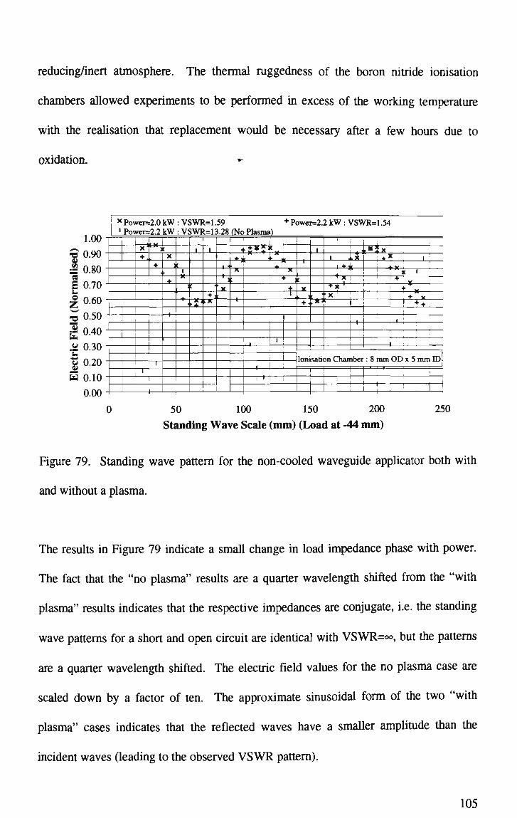
reducing/inert atmosphere. The thermal ruggedness of the boron nitride ionisation
chambers allowed experiments to be performed in excess of the working temperature
with the realisation that replacement would be necessary after a few hours due to
oxidation.
1.00 0.90
£ 0.80 cs
E u o Z
0.70 0.60 0.50
g 0.40 a 0.30
0.20 0.10 0.00
TJ
"oS fa JU
"E fa
xPower=-2.0kW:VSWR=1.59 + Power=2.2kW: VSWR=1.54 ! ' Power=2.2 k W : VSWR=13.28 (No Plasma)
x' • H
1
>
<K>
+ •I
1
1 —
c X .
(•
+
c 1
»
1
1
c
h*1
1
1
Irt-IX
| H
'* Fx c
!
Ix1 •i • / X f
I
„ f
-5*.. •f 1.
1 j 1
j. i !
* 4
1
*• >
t c X
I
I . : '
l«?x ,.s + ,,
i
*i" + C ' ^ , _ - + '
. 1
+ i t I
* * i
L* - ' ' 1 + '
! ' A i ! + • 1 I
i i
[ I : , : ' i i r ' f Ionisation Chamber : 8 m m O D x S m m ID
!
j
> i
i i I 1 ! !
— 1 — 1 — 1 — 1 — 1 , — 1 — ,
50 100 150 200 Standing Wave Scale (mm) (Load at -44 m m )
250
Figure 79. Standing wave pattern for the non-cooled waveguide applicator both with
and without a plasma.
The results in Figure 79 indicate a small change in load impedance phase with power.
The fact that the "no plasma" results are a quarter wavelength shifted from the "with
plasma" results indicates that the respective impedances are conjugate, i.e. the standing
wave patterns for a short and open circuit are identical with VSWR=-<>, but the patterns
are a quarter wavelength shifted. The electric field values for the no plasma case are
scaled down by a factor of ten. The approximate sinusoidal form of the two "with
plasma" cases indicates that the reflected waves have a smaller amplitude than the
incident waves (leading to the observed V S W R pattern).
105

Figure 80 is a most informative graph. The results indicate a steady change in the load
impedance magnitude and phase as the sliding probe position is increased from 4 mm to
68.2 mm. The fact that the 75.2mm results are almost a quarter wave shifted, from the
68.2 mm results, means that the impedance has changed sign, i.e. a resonance has been
passed. The resonance point is the point where maximum power is being transferred to
the plasma and the applicator is operating at peak efficiency. Knowledge of the
resonance point is very important in applicator design since it is the ideal operating
position for the applicator system. The ionisation chamber used in this experiment had
an O.D. and I.D. of 8 and 5 mm respectively.
**•-%
TJ 0) ft "rt
s O 55 TJ 0)
IZ u r .
u ii
5
10.00
9.00
8.00
7.00
6.00
5.00
4.00
3.00
2.00
1.00
0.00
* 4.0mm * 13.2mm — 2 3 . 2 m m * 33.2mm 43.2mm 53.2mm 63.2mm 68.2mm 75.2mm
,i
i\
>
• 7
'/w-
1
** .*. t
>< • r * * !_-> i
e „ * i '
'*< 1
^
C
1
' * • <
4 j i r
4 < >
J
c
t .-•;
1
'
/' ;' ! • • - • k?
-< ••'j
» /V *
••
:
\ •j
4f <;
t
9> *'•« P\
N
!
U-, {*J '•~v.
\
l -!Y' f-~i
•''"•.''
j,* V-. -\ \
f
* ' • '
'•*.,
j I •• :>x
_1 »'
/. .• •
,J' • .X
1
i ,'A
't'< 7-
i ).
'. J
X L_ i
xJ
, •••
1 _ i « • • *
1
i
50 100 150 200
Standing Wave Scale (mm) (Load at -66 m m )
250
Figure 80. Standing wave pattern as a function of load-sliding short distance.
106

35
30
25
g 20
£ 15
10
0
i *
!"
+
,
Yl/irl-
1
Wltii nosma
No Plasma
# •
1 • i
i
i
i • i
i
i
.
•
\
•
•
• • i
i
•
•
i 1 1
i
;
4
0 10 20 30 40 50 60 70 80 90
Distance between load & sliding short (mm)
Figure 81. VSWR as a function of load-sliding short distance.
Figure 81 shows the VSWR as a function of load-sliding short distance for the
waveguide applicator both with and without the plasma present and for a ionisation
chamber with an O.D. and I.D. of 8 and 5 m m respectively. This graph accurately
demonstrates the resonance previously mentioned as does Figure 88. In fact, there is a
shift in resonance of approximately 4 m m between the "with plasma" and "no plasma"
cases signifying an increase in the resonant frequency of the cavity when the plasma is
present. Also note the sharpness of the resonance dip in the "no plasma" graph
compared to the "with plasma" graph. This sharpness reveals that the quality factor of
the cavity, Q is greater in the absence of a plasma. A broad resonance peak is of benefit
when constructing an applicator since cavity dimensions are not as critical and the
applicator is less sensitive to drifts in the driving frequency.
Figure 82 shows the VSWR as a function of microwave power for powers between 2.0
and 3.4 k W . The discharge gas was argon with a flow rate of 15 litres per minute and
107

the O.D. and I.D. of the ionisation chamber was 9.6 m m and 6.0 m m respectively. As
can be seen from the graph, the VSWR appears to have a slight dependence on
microwave power and decreases by about 5 % from a power of 2.0 kW to a power of 3.4
kW. This result is significant since it means the applicator does not have to be re-tuned
if the operating power is altered. However, this dependence may be a function of the
way in which the experiment was performed since the applicator was not re-tuned for a
minimum reflected power after each increment of forward power. This issue of re-
tuning after each alteration in operating conditions is addressed during VSWR
determination experiments found later in this Chapter. In operation, it is very difficult
to tune the applicator accurately since a small change in the sliding short position can
lead to a dramatic change in the VSWR as can be seen from Figure 81.
1.70
1.60
1.50
S 1.40
> 1.30
1.20
1.10
1.00
• ] g 1 II 1 1 , 1.
I I i I ~-=Ezy: i t i : J :
1.9 2.1 2.3 2.5 2.7 2.9 3.1
Microwave Power (kW) 3.3 3.5
Figure 82. V S W R as a function of microwave power.
108

1.80
1.70
1.60
x 1.50
> 1.30
1.20
1.10
1.00
i I I t t -*-. : , I = = - • * • • ,
1 II II 1 ! i i , ; r
I II " ! ! I : M ._44 ; , ; • i i =: f 1 ! ' ' ' : ' : II ! , ; , , , ,
0 5 10 15 20 25 30 35 40 Discharge Gas Flow Rate (litres per minute)
Figure 83. VSWR as a function of discharge gas flow rate.
Figure 83 shows the V S W R as a function of discharge gas flow rate for flow rates of
between 5.0 and 37.5 litres per minute. Again the discharge gas was argon and the O.D.
and I.D. of the ionisation chamber was 9.6 m m and 6.0 m m respectively. This graph
shows a definite discontinuity in the curve occurring at a gas flow rate of 30 litres per
minute. This discontinuity was due to a partial failure of the ionisation chamber
because of oxidisation from operation at elevated temperatures. As can be seen from
Figure 83, the V S W R increases almost linearly with gas flow rate. Again, this
dependence may not represent the true effect since the applicator was not re-tuned after
each increment in gas flow rate. What this Figure does show however, is that the
plasma does change its behaviour with increasing gas flow rate when no other
parameters are varied.
An important note should be made here. Whenever quantitative experiments are to be
performed, it is imperative that the system is re-tuned after each variation in external
109

conditions otherwise ambiguities can occur in the experimental data that lead to
erroneous conclusions. To overcome any ambiguity that may be evident in Figure 82
and Figure 83, both experiments were redone and the results given in Figure 84 and
Figure 85. During the experiment, each time the power or gas flow rate was
incremented, the applicator was re-tuned to give a minimum in reflected power. This
ensures that variations in V S W R are a result of changes in power or gas flow rate and
not a result of cavity detuning. The results given in Figure 82 and Figure 83 are still
important since in practice one can still get these variations and conditions without re-
tuning.
1.7-1 1 1 1 1 1 1 1 1 1 1 : • :
u = = 4 > = I 1 : " 1.5 • 1 1 1 ' j
* 1.4 •] 1 1 l ' 1 £ , , 1 , , . 1 1 1 : , 1 > 1.3 ' 1 r-1-] | 1 ' 1
1.2 " 1 '
0.5 0.7 0.9 1.1 1.3 1.5 1.7 1.9
Microwave Power (kW)
Figure 84. V S W R as a function of microwave power for a re-tuned cavity.
In Figure 84, the VSWR appears to increase to a plateau as the power is increased. This
may be because of a levelling-off of one of the plasma parameters such as temperature
or even as a result of non-linear heating with power of the ionisation tube. Figure 85
reveals the linear dependence of V S W R on discharge gas flow rate. Neglecting the
110

wayward points corresponding to 5 and 25 litres per minute, a linear fit to the data
points yields an R squared value for this curve of 0.95. The decrease of V S W R with
increasing gas flow rate may be due to the cooling effect of the extra gas or the altering
of the gas flow dynamics with increasing flow rate. Regardless of the mechanism, the
trend in Figure 85 is unmistakable.
C/5
1.46
1.45
1.44
1.43
1.42
1.41
1.4
1.39
1.38
1.37
1.36
1.35
1
•
1
I
1 I
1
1
1
•
1
]
• 1 1
' !
! i i ! ! '
'
i ' '
1
1
1
" I T a I 1
, i
2.5 7.5 12.5 17.5 22.5 27.5
Discharge Gas Flow Rate (litres per minute)
32.5
Figure 85. V S W R as a function of discharge gas flow rate for a re-tuned cavity
The data given in Figure 82 and Figure 84 shows well the ambiguity that can occur
when the system is not re-tuned between each experiment. To reveal the true nature of
the effect of power on VSWR, the following experiment was performed. The
microwave power was set at a predetermined level, the sliding short at a predetermined
position and the VSWR recorded. The sliding short position was incremented 0.3 mm
closer to the resonance point and the VSWR recorded again. This process of increment
and measure was repeated until the resonance point had been passed. The sliding short
was re-zeroed and the microwave power level incremented to a new value. The process
111
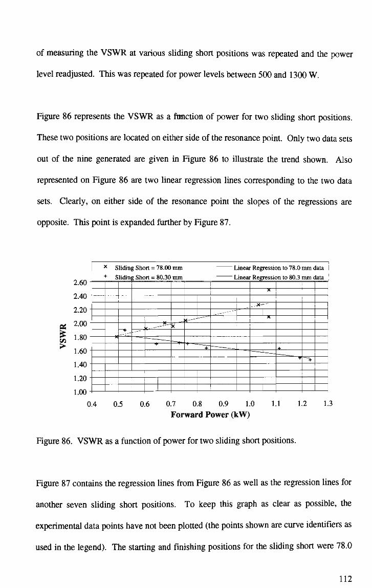
of measuring the V S W R at various sliding short positions was repeated and the power
level readjusted. This was repeated for power levels between 500 and 1300 W .
Figure 86 represents the VSWR as a function of power for two sliding short positions.
These two positions are located on either side of the resonance point. Only two data sets
out of the nine generated are given in Figure 86 to illustrate the trend shown. Also
represented on Figure 86 are two linear regression lines corresponding to the two data
sets. Clearly, on either side of the resonance point the slopes of the regressions are
opposite. This point is expanded further by Figure 87.
>
2.60
2.40
2.20
2.00
1.80
1.60
1.40
1.20
1.00
x snaing snort = VH.UU m m + Slidin
*
z, snort = SU.JU m m
K "
+
__*£-X
"•C* '—
Linear Regression to /8.U m m data
Linear Regression to 80.3 m m data
^~+~
1 1
__ ----" x-
X
X
. '
+ • * >
0.4 0.5 0.6 0.7 0.8 0.9 1.0
Forward Power (kW) 1.1 1.2 1.3
Figure 86. V S W R as a function of power for two sliding short positions.
Figure 87 contains the regression lines from Figure 86 as well as the regression lines for
another seven sliding short positions. T o keep this graph as clear as possible, the
experimental data points have not been plotted (the points shown are curve identifiers as
used in the legend). The starting and finishing positions for the sliding short were 78.0
112
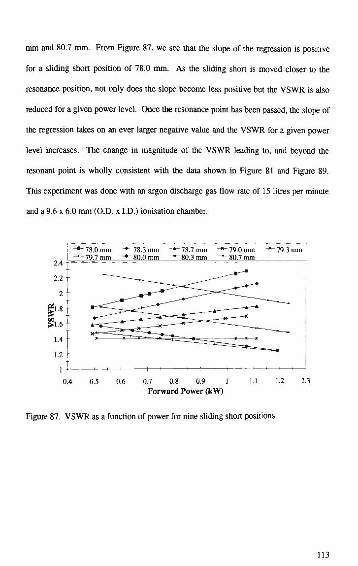
m m and 80.7 m m . From Figure 87, we see that the slope of the regression is positive
for a sliding short position of 78.0 mm. As the sliding short is moved closer to the
resonance position, not only does the slope become less positive but the VSWR is also
reduced for a given power level. Once the resonance point has been passed, the slope of
the regression takes on an ever larger negative value and the VSWR for a given power
level increases. The change in magnitude of the VSWR leading to, and beyond the
resonant point is wholly consistent with the data shown in Figure 81 and Figure 89.
This experiment was done with an argon discharge gas flow rate of 15 litres per minute
and a 9.6 x 6.0 mm (O.D. x I.D.) ionisation chamber.
2.4
2.2-
2"
|l.8
£l.6
1.4
1.2
1
78.0 m m 79.7 m m
78.3 m m 80.0 m m
78.7 mm 80.3 mm
79.0 mm 80.7 m m
79.3 mm
H 1 1 r-
0.4 0.5 0.6 0.7 0.8 0.9 1
Forward Power (kW)
1.1
H 1 r-
1.2 1.3
Figure 87. V S W R as a function of power for nine sliding short positions.
113

170 '—?
1 •5-c o '•S 08
8 J 08
a IS 5 &
3 "3 >
160
150
140
130
120
110 100
90
80
i
j
i ! ' . , ; ' • • ! '
i
- r
i
•
- i '
r ! : i i i .• ; : ! | i i ' ' • ; • !
1 j | i , i i | ' :
: - • i ! i
! ! i i ! ' , : I
i • i I I !
T-• :
1 j ! ! 1 :
1 S"i_! -_ • : I 1 ! ! : - » ] - * • • •
70 71 72 73 74 75 76 77 78 79 80 81 82 83 84 85 86
Sliding Short-Load Distance ( m m )
Figure 88. Voltage maxima position as a function of sliding short-load distance.
The data in Figure 88 was generated using argon as the discharge gas with a flow rate of
7.5 litres per minute and a ionisation chamber with an O.D. and I.D. of 9.6 and 6.0 mm
respectively. The microwave power was set at 700 W and not altered for the duration of
the experiment. The sliding short-load distance was set at 70 mm and the position of a
voltage maximum on the slotted scale recorded. The sliding short was then moved a
quarter turn, 0.31 mm, closer to the load and the position of the same voltage maxima
recorded. This procedure was repeated until the sliding short-load distance was 85.5
mm. This span was necessary to encapsulate the resonance condition which, from
Figure 88, occurred at a sliding short-load distance of approximately 79.9 mm. Note
that the location of the resonance condition in Figure 88 is different from that in Figure
81. This is because of a number of factors, such as ionisation chamber dimension,
discharge gas flow rate and microwave power level. Specifically, for Figure 81 the
values for each were 8x5 mm, 20 l/min and 2.2 kW and Figure 88 the values were 9.6
x 6 mm, 7.5 l/min and 700 W.
114
A hitherto unmentioned benefit of the cavity applicator over the coaxial applicator is the
reduced leakage of microwave radiation. Prior to striking a plasma, the coaxial
applicator is essentially just an antenna radiating into free space. The situation does not
change drastically after the plasma ha*, been struck. The effect of the plasma is to
reduce the radiated levels of microwave radiation as this radiation loses energy to the
plasma. For the case of the cavity applicator, no microwave radiation escapes when
there is no plasma since the microwaves are completely enclosed within the cavity.
After the plasma has been initiated, the radiated levels of microwaves increase due to
the finite conductivity of the plasma. Were the plasma to be a perfect conductor then it
would act as an efficient antenna, or a waveguide to coaxial transition, and radiate
microwave energy from within the cavity to free space. To determine the effect of these
radiative losses on the plasma properties, the plasma exit orifice and the discharge gas
inlet were fitted with chokes. The plasma was then initiated and the VSWR determined
as a function of load-sliding short distance. The results, shown in Figure 89, are for a
ionisation chamber with an O.D. and I.D. of 9.6 and 6.0 mm respectively. The
discharge gas was argon with a flow rate of 7.5 litres per minute and the microwave
power level was set at 700W. As can be readily seen from Figure 89, the external
chokes had no effect on the VSWR measured. This result is important since it means
that an effective microwave plasma welder can be fitted with chokes to minimise
microwave leakage without impacting on the operational characteristics of the device.
115
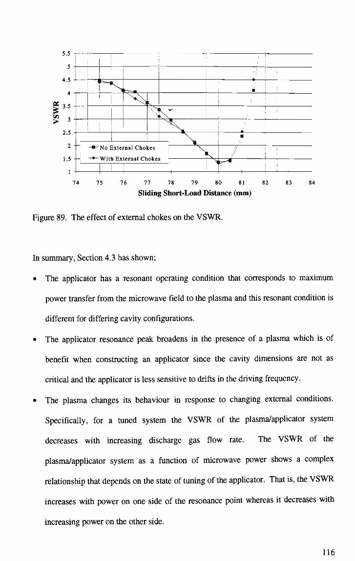
: .' ! '
" * \ »
-*- No External Chokes
-•-With External Chokes
1 H 1
;/ j
! * i
• i -
• •
./ i
1 1— — i — i — •
74 75 76 77 78 79 80 81 82 83 84
Sliding Short-Load Distance (mm)
Figure 89. The effect of external chokes on the V S W R .
In summary, Section 4.3 has shown;
• The applicator has a resonant operating condition that corresponds to maximum
power transfer from the microwave field to the plasma and this resonant condition is
different for differing cavity configurations.
• The applicator resonance peak broadens in the presence of a plasma which is of
benefit when constructing an applicator since the cavity dimensions are not as
critical and the applicator is less sensitive to drifts in the driving frequency.
• The plasma changes its behaviour in response to changing external conditions.
Specifically, for a tuned system the V S W R of the plasma/applicator system
decreases with increasing discharge gas flow rate. The V S W R of the
plasma/applicator system as a function of microwave power shows a complex
relationship that depends on the state of tuning of the applicator. That is, the V S W R
increases with power on one side of the resonance point whereas it decreases with
increasing power on the other side.
116

• External chokes have no effect on the plasma properties and hence the measured
VSWR. This is an important practical result since it means that an effective
microwave plasma welder can be fitted with chokes to minimise microwave leakage
without impacting on the operational characteristics of the device.
4.4 Electric Circuit Model of the Waveguide Applicator.
To model the electrical properties of the plasma/applicator system, it is necessary to
measure the VSWR as a function of load-sliding short distance, Ls. This involves not
only measuring the load-sliding short distance and minimum and maximum field
intensities but the positions of those minima and maxima with respect to the load.
Incident • A O O 1
V\n Source
i _ 0 O 1 Reflected < A
Figure 90. Electrical circuit representation used in microwave plasma diagnostics.
Once the VSWR and the distance to the load, d, are known (shown schematically in
Figure 90), a Smith Chart is employed to determine the impedance of the load as seen
from the point A -A. Combining this with knowledge of how the plasma behaves
electrically will then allow an electrical circuit analogue to be developed.
"load
117

Once the data has been plotted on the Smith chart and the normalised load impedance,
ZLoad, and load admittance, Yu^, determined, all that is needed is to subtract the
admittance presented by the sliding short, YstUb, from the load admittance to give the
plasma admittance, Ypiasma. i.e. -*-
v = LLoad
1
'Load
x PUxsmar * Stub
The data used to derive the electrical circuit model of the plasma/applicator system is
shown graphically in Figure 91. An alumina ionisation chamber with an O.D. and I.D.
of 9.6 and 6.0 mm respectively was used for this experiment.
80
70
H 60
| 50
u 40
J? 30
20
10
<> i
II 1
• % Power Reflected
1"VSWR
P=0.6 kW, Gas How="
* A >
4 *
• i
L — j - . !
-J1 - . - •
i
'.5 l/min p
•
•
•
• • •
i
1 II « |
•
•
•
1 <
i '
i
i
' •
i
17
15
13
11
(/}
75 76 77 78 79 80 81 Sliding Short-Load Distance (mm)
82 83
Figure 91. Percentage reflected power and V S W R as a function of sliding short
position.
This data has been plotted on the Smith Chart shown in Figure 92 along with reference
points denoting the starting and finishing points of the sliding short circuit traverse.
118

Recall that the sliding short circuit is at zero on the "load-sliding short distance" scale
and that the distance between the load and the sliding short circuit is denoted by Ls. In
Table 10, Ls and VSWR were experimentally measured, ZLoad and YLoad determined from
the Smith Chart shown in Figure 92, and YStUb, Ypi-sma, and Zpiasma calculated using
^ = - ; ' c o t ( ( 5 Ls) and P - . ^8
where A,g is the waveguide wavelength.
119
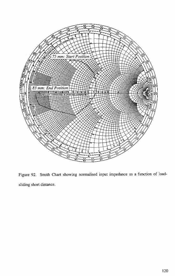
Figure 92. Smith Chart showing normalised input impedance as a function of load-
sliding short distance.
120
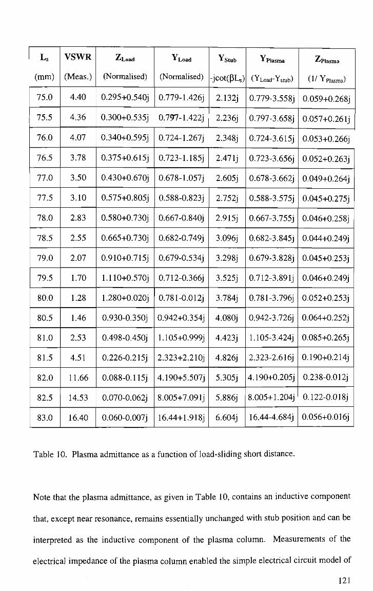
Ls
(mm)
75.0
75.5
76.0
76.5
77.0
77.5
78.0
78.5
79.0
79.5
80.0
80.5
81.0
81.5
82.0
82.5
83.0
VSWR
(Meas.)
4.40
4.36
4.07
3.78
3.50
3.10
2.83
2.55
2.07
1.70
1.28
1.46
2.53
4.51
11.66
14.53
16.40
--'Load
(Normalised)
0.295+0.540J
0.300+0.535J
0.340+0.595J
0.375+0.615j
0.430+0.670J
0.575+0.805J
0.580+0.730J
0.665+0.730J
0.910+0.715J
1.110+0.570J
1.280+0.020J
0.930-0.350J
0.498-0.450J
0.226-0.215j
0.088-0.115j
0.070-0.062J
0.060-0.007J
YLoad
(Normalised)
0.779- 1.426J
0.797-1.422j
0.724-1.267J
0.723- 1.185J
0.678-1.057J
0.588-0.823J
0.667-0.840J
0.682-0.749J
0.679-0.534J
0.712-0.366J
0.781 -0.012j
0.942+0.354J
1.105+0.999J
2.323+2.210J
4.190+5.507J
8.005+7.09 lj
16.44+1.918j
Ystub
-jcot(PLs)
2.132J
2.236J
2.348J
2.47 lj
2.605J
2.752J
2.915J
3.096J
3.298J
3.525J
3.784J
4.080J
4.423J
4.826J
5.305J
5.886J
6.604J
* Plasma
(YLoad" Ysmb)
0.779-3.558J
0.797-3.658J
0.724-3.615J
0.723-3.656J
0.678-3.662j
0.588-3.575J
0.667-3.755j
0.682-3.845J
0.679-3.828J
0.712-3.891J
0.781-3.796J
0.942-3.726j
1.105-3.424j
2.323-2.616j
4.190+0.205J
8.005+ 1.204J
16.44-4.684j
-^Plasma
(1/Ypiasma)
0.059+0.268J
0.057+0.26 lj
0.053+0.266J
0.052+0.263J
0.049+0.264J
0.045+0.275J
0.046+0.258J
0.044+0.249J
0.045+0.253J
0.046+0.249J
0.052+0.253J
0.064+0.252J
0.085+0.265J
0.190+0.214j
0.238-0.012J
0.122-0.018j
0.056+0.016j
Table 10. Plasma admittance as a function of load-sliding short distance.
Note that the plasma admittance, as given in Table 10, contains an inductive component
that, except near resonance, remains essentially unchanged with stub position and can be
interpreted as the inductive component of the plasma column. Measurements of the
electrical impedance of the plasma column enabled the simple electrical circuit model of
121
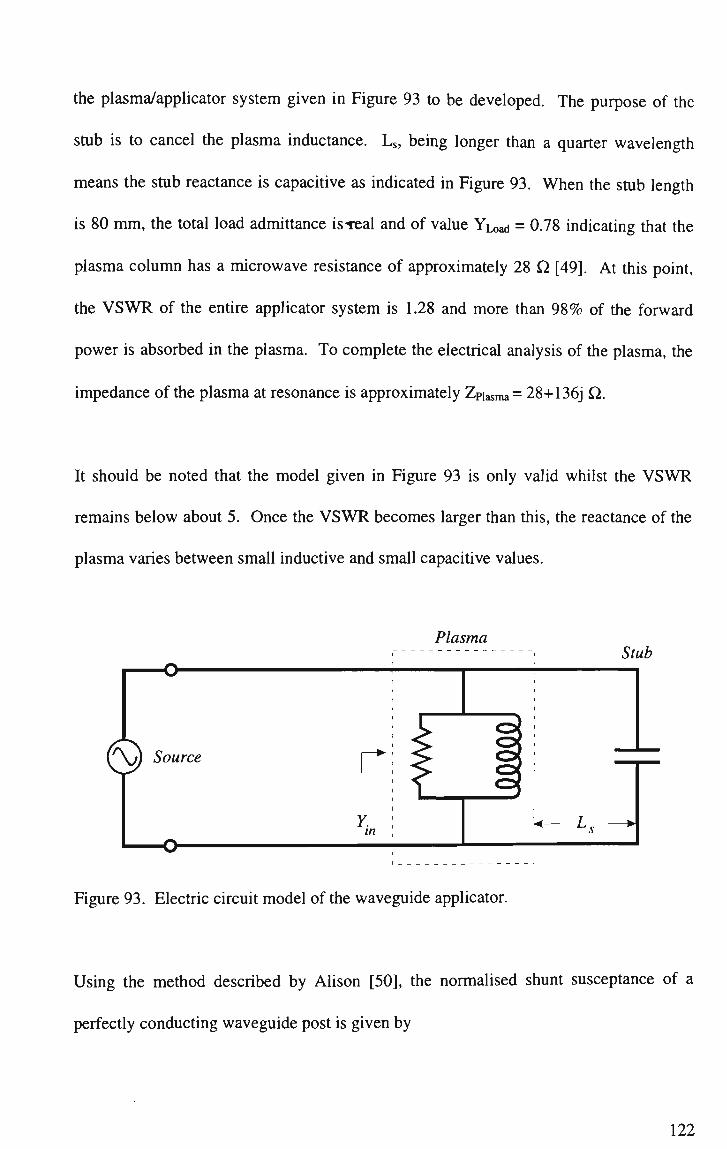
the plasma/applicator system given in Figure 93 to be developed. The purpose of the
stub is to cancel the plasma inductance. Ls, being longer than a quarter wavelength
means the stub reactance is capacitive as indicated in Figure 93. When the stub length
is 80 mm, the total load admittance is real and of value YLoad = 0.78 indicating that the
plasma column has a microwave resistance of approximately 28 Q [49]. At this point,
the VSWR of the entire applicator system is 1.28 and more than 98% of the forward
power is absorbed in the plasma. To complete the electrical analysis of the plasma, the
impedance of the plasma at resonance is approximately Zpiasma= 28+136j Q.
It should be noted that the model given in Figure 93 is only valid whilst the VSWR
remains below about 5. Once the VSWR becomes larger than this, the reactance of the
plasma varies between small inductive and small capacitive values.
Plasma Stub
Figure 93. Electric circuit model of the waveguide applicator.
Using the method described by Alison [50], the normalised shunt susceptance of a
perfectly conducting waveguide post is given by
122

-2X 8 • 2
-sin fnx^
b~ a a J-ln ^ 4a . f^W
V nd
sin nx
\avj - 2 sin'
fnx^ r
\a J
nd\
K7Xj
where the dimensions are defined as:
d • <—
M
^
a
- x — >
•
A
b
1 v
Figure 94. Dimensions for inductive susceptance calculations.
Modelling the plasma column as a perfectly conducting wire of diameter 6 mm (equal to
the inside diameter of the ionisation chamber) stretched across the waveguide and using,
1) ^g=0.1744 m
2) a=0.086m
3) b=0.043m
4) x=0.043m
5) X=0.1224 m
123

the calculated value for the inductive susceptance at resonance is -4.52. This compares
quite favourably with the experimental value of -3.796, for example, the model predicts
that a wire diameter of 5.07 mm, leads to a normalised susceptance at resonance
identical to the experimentally determined value. This result further justifies the validity
of the electrical circuit model of the plasma/applicator system given in Figure 93.
4.5 Plasma Impedance Measurements.
Following the method prescribed in Section 4.4 or the method of Ramo et al. [51], it is
relatively straightforward to generate the plasma impedance as a function of the
operating variables of the system. Figure 95 and Figure 96 give the real and imaginary
normalised plasma impedance as a function of sliding short-load distance for the non-
cooled waveguide applicator. This is a graphical representation of the data used to
determine the electric circuit model of the plasma previously given in Table 10. As can
be readily seen from Figure 95, the normalised real impedance of the plasma is
approximately constant as resonance is approached. As resonance is passed, the
impedance increases rapidly to achieve a maximum value approximately five times
greater than when at resonance. We see from Figure 91 that this occurs where the
VSWR starts to increase sharply. Figure 96 shows the effect on the imaginary
component of the normalised impedance as the sliding short-load distance is varied.
When the sliding short-load distance is 82 mm, the plasma is a purely resistive load and
has a microwave resistance of approximately 140 £2.
Figure 97 and Figure 98 give the normalised plasma impedance (real and imaginary
respectively) as a function of microwave power. We see from these two graphs that the
124
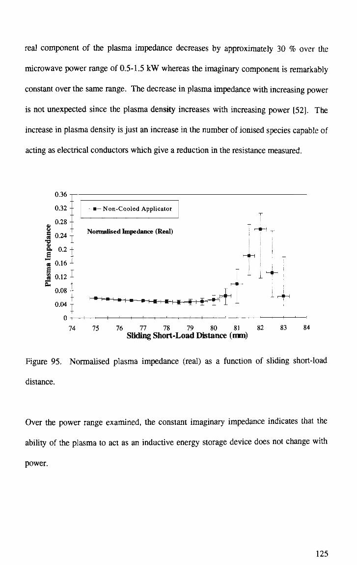
real component of the plasma impedance decreases by approximately 30 % over the
microwave power range of 0.5-1.5 kW whereas the imaginary component is remarkably
constant over the same range. The decrease in plasma impedance with increasing power
is not unexpected since the plasma density increases with increasing power [52]. The
increase in plasma density is just an increase in the number of ionised species capable of
acting as electrical conductors which give a reduction in the resistance measured.
u u e 08
•8 a. E M 03
S ce 08
0.36
0.32 -
0.28 -
0.24-
0.2-
0.16
0.12 -f
0.08
0.04
0
Non-Cooled Applicator
Normalised Impedance (Real)
T
1 1
* + ^ - + * + § + i + r t K£ -I 1 H -> 1 1 1
74 75 76 77 78 79 80 81
Sliding Short-Load Distance (mm) 82 83 84
Figure 95. Normalised plasma impedance (real) as a function of sliding short-load
distance.
Over the power range examined, the constant imaginary impedance indicates that the
ability of the plasma to act as an inductive energy storage device does not change with
power.
125

-)
u s 08
"8 a E 08
E 08
0.35
0.3
0.25
0.2-
0.15 -
0.1 -
0.05
0
-0.05
-0.1
Normalised Impedance (imaginary)
Non-Cooled Applicator
-i h -i 1 -
74 75 76 77 78 79 80 81 82
Sliding Short-Load Distance (mm) 83 84
Figure 96. Normalised plasma impedance (imaginary) as a function of sliding short-
load distance.
*~ Non-Cooled Applicator
* — I 1 vr i
Normalised Impedance (Real) ) 1 1 1 1 1 1 1 1 1 1 1 1 1 1 1 1 1 1 1 1 1 1 1—H 1 1 1 1-
0.4 0.6 0.8 1 1.2
Microwave Power (kW) 1.4 1.6
Figure 97. Normalised plasma impedance (real) as a function of microwave power.
126

0.3
0.25 " u u § 0.2
"8 a I 0.15 t 08
S o.i 0.05 "
0.4
i
~"~~ Non-Cooled Applicator Normalised Impedance (Imaginary)
- t — i — i — i — i — i — i — | — i — l — y — i — ! — i — i — i — i — i -
0.6 0.8 1 1.2
Microwave Power (kW) 1.4 1.6
Figure 98. Normalised plasma impedance (imaginary) as a function of microwave
power.
Figure 99 and Figure 100 give the normalised plasma impedance (real and imaginary
respectively) as a function of discharge gas flow rate for a 0.7 kW plasma. The results
shown indicate that both the microwave resistance and the inductive reactance of the
plasma increases with increasing gas flow rate. As will be shown later in this Chapter,
the plasma temperature decreases with increasing flow rate thereby decreasing the
number of charge carriers in the plasma which leads to an increase in microwave
resistance of the plasma. The increase in the inductive reactance of the plasma in Figure
100 and the constant value in Figure 98 can be explained in terms of the gas density
within the ionisation chamber. As the discharge gas flow rate is increased, the pressure
and subsequently the gas density inside the ionisation tube increases. It is not
unreasonable to hypothesise that the inductive reactance of the plasma is a function of
gas density since a greater energy storage capacity would require a greater number of
storage mediums. This cannot be the whole story however since as the temperature of
127

the plasma increases, with increasing power, one would expect the gas density to
decrease thereby reducing the reactance. This clearly does not happen in Figure 98 so
there may be more than one mechanism leading to the reactance of the plasma.
0.24
I 08
"8 ft
£ 08
E ce OS Pr
0.2
0.16 -
0.12 -
0.08
0.04 -Non-Cooled Applicator Normalised Impedance (Real)
H 1 1 1 1 1 1 1 1 h H 1 1 1 1 1 1 h -I 1 1 1 1 1 V-
0 2 4 6 8 10 12 14 16 18 20 22 24 26 28 30 32
Discharge Gas Flow Rate (litres per minute)
Figure 99. Normalised plasma impedance (real) as a function of discharge gas flow rate
for a 0.7 kW plasma.
0.35
0.3-
v H 0.25 -
"8 5. 0.2-
E g 0.15 -
E £ 0.1-0.05 "
0
T -*- i
Non-Cooled Applicator Normalised Impedance (Imaginary)
•A 1 1 1 1 h -I 1 1 1 1 1 1 1 1 1 1 1 1 1 i I ' 1 1 -
2 4 6 8 10 12 14 16 18 20 22 24 26 28 30 32
Discharge Gas Flow Rate (litres per minute)
Figure 100. Normalised plasma impedance (imaginary) as a function of discharge gas
flow rate for a 0.7 kW plasma.
128

4.6 V S W R Measurements on the Water-Cooled Waveguide Applicator.
Section 4.3 covered VSWR measurements on the non-cooled waveguide applicator and
Section 4.4 considered the electric circuit model for the waveguide applicator derived
from these measurements. This section presents VSWR data obtained for the water-
cooled version of the waveguide applicator. Prior to commencing this phase of
experimentation, a more stable and reliable magnetron power supply was purchased.
An estimation of experimental errors is also given where the word "estimation" is
carefully chosen since it is very difficult to replicate some of the parameters that may
affect the plasma properties for each experiment. For example, the rate of change of
temperature of the applicator is dependent on radiative and convective losses to the
surrounding atmosphere. As there was no control over the temperature, humidity or
turbidity of the atmosphere, it is reasonable to assume that the data has systematic or
non-estimatible errors. A source of random or non-estimatible error is the alignment of
the short circuit tuning plunger. The plunger has copper beryllium fingers attached to
the periphery to ensure a good electrical contact. As the direction of motion of the
plunger is changed, play in the connecting shaft allows the face of the plunger to move
out of square with respect to the waveguide. This misalignment could lead to noticeable
errors if the plunger were located at the resonant position. For example, this may be the
reason for the wayward data point in Figure 101 corresponding to 1.75 kW on the 3
litres/minute curve.
129

5 litres/min
0.5 1.5 2 2.5 3 3.5 4
Microwave Power (kW) 4.5 5.5
Figure 101. V S W R as a function of microwave power for 5 separate discharge gas flow
rates.
Figure 101 represents the V S W R as a function of microwave power for discharge gas
flow rates between 3 and 7 litres per minute. Without exception, the VSWR reduces
with increasing power for a fixed gas flow rate. Error bars have been omitted from this
Figure for clarity. Figure 102 shows the VSWR as a function of discharge gas flow rate
for a 3 kW plasma. Two curves are represented as an indication of repeatability.
Firstly, the VSWR was measured for a flow rate decreasing from 10 to 1 litres/minute
and then the VSWR measured whilst increasing the gas flow rate from 1 to 10
litres/minute. These findings show that the curves are generally the same within the
experimental limits and are also in agreement with the non-cooled applicator case. This
result is important because it shows that within experimental limits the method of data
collection has no bearing on the outcome of the experiment.
130

2
1.9
1.8
1.7
1.6 rt
11.5 >
1.4
1.3
1.2-
1.1 -
1
1 to 10 litres/minute
10 to 1 litres/minute
H 1 r- H 1 1 1 1 1 1 1 r-
0 2 3 4 5 6 7 8 9 Discharge Gas Flow Rate (litres per minute)
10 11
Figure 102. V S W R as a function of discharge gas flow rate for a 3 k W plasma.
4.7 Plasma Impedance Measurements on the Water-Cooled Waveguide
Applicator.
This section is similar to Section 4.5 in that it deals with the plasma impedance as a
function of external variables such as microwave power and discharge gas flow rate.
However, the data presented here is for the water-cooled waveguide applicator whereas
the data presented in Section 4.5 was for the non-cooled version. This difference was
made obvious because the range over which either applicator can operate is different
and thus some aspects of the data generated are not directly comparable between the two
designs. Wherever possible however, comparable experimental data from each
applicator is presented on the one Figure.
Figure 103 and Figure 104 show the normalised plasma impedance (real and imaginary
respectively) as a function of discharge gas flow rate for a 3 kW plasma. Again, two
sets of experimental data were generated. The first, by decreasing the gas flow rate from
131

10 to 1 litres/minute and the second, by increasing it from 1 to 10 htres/minute. As with
Figure 102, the results for the two curves on each of these Figures are in general
agreement within experimental error. The normalised plasma impedance (real), as
shown in Figure 103, increases in magnitude by between two and three times over the
discharge gas flow range of 1 to 10 litres/minute whereas the normalised impedance
(imaginary), as shown in Figure 104, decreases by about 20%. Another thing to note
about Figure 104 is that the curve shows the same general trends as the VSWR as a
function of discharge gas flow rate shown in Figure 102. The error bars were calculated
by determining the maximum possible excursions for the impedance about the measured
values as calculated from errors in variable determination. This method of error
determination results in different values for the positive and negative error bars as seen
graphically in Figure 95 and Figure 96.
0.32
0.28 -9»
s 0.24 -f 08
8. 0.2- E i - i 5 0.16 -f E 012 T
J-
0.08 -
0.04 4-
1 to 10 (Real) 10 to 1 (Real)
Normalised Impedance (Real) r — | 1 1 1 1 1 1 1 1
0 1 2 3 4 5 6 7 8 9 10 11 Discharge Gas Flow Rate (litres per minute)
Figure 103. Normalised plasma impedance (real) as a function of discharge gas flow
rate for a 3 kW plasma.
132
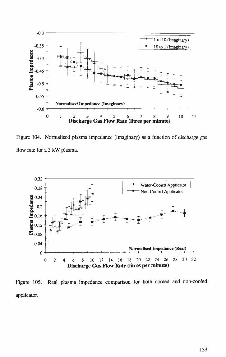
0.3
-0.35 1
u
Jj -0.4 1 Q.
I -0.45 1 08
E 3 -0.5 H
-0.55 -
-0.6
~* 1 to 10 (Imaginary)
* 10 to 1 (Imaginary)
Normalised Impedance (Imaginary) i — i — i — i — i — i — i — i — i — i — i — H r-
0 1 2 3 4 5 6 7 8 9 10 11 Discharge Gas Flow Rate (litres per minute)
Figure 104. Normalised plasma impedance (imaginary) as a function of discharge gas
flow rate for a 3 kW plasma.
' Water-Cooled Applicator
Non-Cooled Applicator
J.-4—i
Normalised Impedance (Real) \ — i — i — i — i — i — i — i — i — i — i — i — i — i — i — i — i — i — i — i — i
0 2 4 6 8 10 12 14 16 18 20 22 24 26 28 30 32 Discharge Gas Flow Rate (litres per minute)
Figure 105. Real plasma impedance comparison for both cooled and non-cooled
applicator.
133

Figure 105 and Figure 106 shows the real and imaginary plasma impedance
comparisons for both cooled and non-cooled applicator, respectively. From Figure 105
it can be seen that the trends for impedance as a function of gas flow rate are identical,
i.e. the normalised real plasma impedance increases with increasing discharge gas flow
rate though at differing rates for the two applicators. More importantly, the magnitude
of the impedance is the same order of magnitude indicating that similar processes are
occurring within each applicator.
0.4 T~
FS___ffl ffl m ffl ffi ffl 8- ® * m
• Water-Cooled Applicator * Non-Cooled Applicator
-0.5"; ----I-T-7j}££g; Normalised Impedance (Imaginary) .0 . 6 "I > 1 ' I ' 1 ' 1 ' 1 ' 1 ' 1 ' 1 ' 1 ' 1 ' ! ' 1 ' ' ' ' ' ' ' '
0 2 4 6 8 10 12 14 16 18 20 22 24 26 28 30 32
Discharge Gas Flow Rate (litres per minute)
Figure 106. Imaginary plasma impedance comparison for both cooled and non-cooled
applicator.
Figure 106 is a most informative graph. Recall that the plasma admittance calculated
for the non-cooled applicator led to the development of an electric circuit model of the
plasma column. In addition, the reactance of the plasma column was inductive and
good agreement was obtained by modelling the plasma as a perfectly conducting wire
stretched across the broadwall of the waveguide. From Figure 106 we see that the
a u B 08 •a a a, E 58
E
0.3 '
0.2--"
o.i -
o --0.1 -
-0.2 -
134

reactance has changed sign for the water-cooled applicator indicating that the plasma
column now has a capacitive reactance as opposed to the inductive reactance of the non-
cooled applicator. The capacitive reactance can be explained by considering the
geometry of the ionisation chamber-water jacket arrangement. In many respects, this
arrangement is identical to a length of coaxial cable with an inner conductor separated
from an outer conductor by an annulus of non-conductor. For the case at hand, the inner
conductor is the plasma, the non-conductor is the boron nitride ionisation chamber and
the outer conductor is the coolant itself. As the coolant was not demineralised, electrical
conduction at 2450 MHz would have been enhanced and the ionisation chamber
arrangement would have acted as a cylindrical capacitor.
0.25
g 0.2 1 s S3
10.15 1 S c 0.1 1
~+— 3 litres/min ~*r~ 6 litres/min
• 4 litres/min "*~" 7 litres/min
5 litres/min
Normalised Impedance (Real)
\X--XV * = *
0.05 " | H * t
0.5 1.5 2.5 3.5
Microwave Power (kW) 4.5 5.5
Figure 107. Normalised plasma impedance (real) as a function of microwave power for
five discharge gas flow rates.
Figure 107 and Figure 108 show the normalised plasma impedance (real and imaginary
respectively) as a function of microwave power for five discharge gas flow rates.
135

Again, error bars have been omitted from these graphs for clarity (the individual plots
with associated error bars corresponding to these curves can be found in Figure 109
through Figure 118). For each gas flow rate, the real plasma impedance increases as a
function of microwave power whereas *he imaginary plasma impedance decreases.
Strictly speaking, the reactance (imaginary component of the impedance) increases or
becomes more negative with increasing power. If we continue with the electrical
analogue, this means that the ability of the plasma to "store" energy increases with
increasing power, as does the microwave resistance. Comparing Figure 107 with Figure
97, it is noted that the plasma impedance vs. microwave power dependency is
significantly different even though the magnitude is similar. This is understandable
when, as noted above, the geometry of the ionisation chamber is different for each
applicator and as such, the electrical properties of the plasma will differ.
-0.2
cu u B 08
-a
a l s
-0.25
-0.3
-0.35 -J
-0.4 -
-0.45 -
-0.5 -
-0.55 -r
-0.6
-i— 3 litres/min -*— 6 litres/min
• 4 litres/min -x— 7 litres/min
5 litres/min
.. Normalised Impedance (Imaginary)
0.5 1.5 2.5 3.5
Microwave Power (kW) 4.5 5.5
Figure 108. Normalised plasma impedance (imaginary) as a function of microwave
power for five discharge gas flow rates.
136

0.2
0.18 1
0.16
8 0.14
a | 0-12 1
E o.i 1 0.08
0.06
0.04
0.02
0
£
0.5
3 litres/min
Normalised Impedance (Real)
1.5 2 2.5 3 3.5 Microwave Power 0-W)
4.5 5.5
Figure 109. Normalised plasma impedance (real) as a function of microwave power for
a discharge gas flow rate of three litres per minute.
4.5
4 1 w w
§ 3.5
I 3 (8
s I 2.5 1
2 -
1.5
0.5
h*-H-*H .. H*d
F=rH+ T
Normalised Impedance (Imaginary)
— i 1 1 1 1 —
1.5 2.5 3.5
Microwave Power (kW)
3 litres/min
^•Si •A 1- H 1
4.5 5.5
Figure 110. Normalised plasma impedance (imaginary) as a function of microwave
power for a discharge gas flow rate of three litres per minute.
137
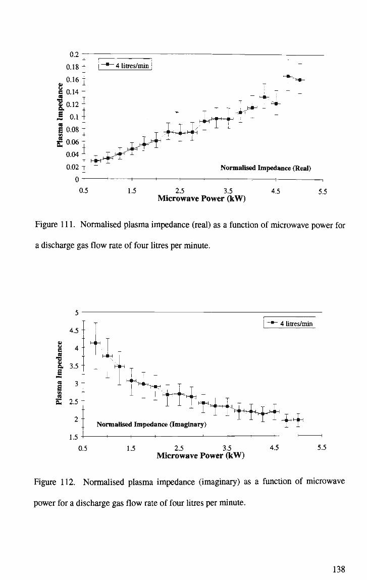
0.2 T
0.18 1
0.16
B 0.14 1
(0.12 -
M 0.11
g 0.08
"*~ 4 litres/min
0.5
T J J r*^
HKf4- T " * ' -i-
Normalised Impedance (Real)
1.5 2.5 3.5
Microwave Power (kW) 4.5 5.5
Figure 111. Normalised plasma impedance (real) as a function of microwave power for
a discharge gas flow rate of four litres per minute.
2
1.5
4 litres/min
Normalised Impedance (Imaginary) I+4H
- I 1
0.5 1.5 2.5 3.5
Microwave Power (kW) 4.5 5.5
Figure 112. Normalised plasma impedance (imaginary) as a function of microwave
power for a discharge gas flow rate of four litres per minute.
138

0.28 T-
0.24 |
g 0.2 08
-3 a 0.16 1
M g 0.12 1 E in
E 0.08 -
5 litres/min
0.04 - H£+^*4 * ***+
£r
Normalised Impedance (Real)
0.5 1.5 2.5 3.5
Microwave Power (kW) 4.5 5.5
Figure 113. Normalised plasma impedance (real) as a function of microwave power for
a discharge gas flow rate of five litres per minute.
4.5
4 -
2 3.5 08
a 3 -S
1 Z5 + ce
O, 2 1.5 4
1
^"SlH^H
T H W>.H
T-HN-I
51itres/rnin
T ^ ^ , Normalised Impedance (Imaginary)
^ ^ f ^
0.5 1.5 2.5 3.5
Microwave Power (kW) 4.5 5.5
Figure 114. Normalised plasma impedance (imaginary) as a function of microwave
power for a discharge gas flow rate of five litres per minute.
139

\J.&* -
0.2-
8 3 0.16 -
"8 B. S 0.12 -08 E S 0.08 -Cu
0.04-
0 -
—•— 6 litres/min
- Ir*
1 1-
~ T
•Jf-H
i 1 —
_ 1
t —
1 ¥
1
_ _ -
*
; v! ^ - - - -
i
Normalised Impedance (Real)
— I 1 1 1
0.5 1.5 2.5 3.5
Microwave Power (kW) 4.5 5.5
Figure 115. Normalised plasma impedance (real) as a function of microwave power for
a discharge gas flow rate of six litres per minute.
4.5
4 -
B 3.5 1 I-1H 08
a, 3 -E
2 2.5 E vi 08
i 2 + 1.5
1
0.5
hT +-HH
T
Normalised Impedance (Imaginary)
'*+.
1.5 2.5 3.5
Microwave Power (kW)
6 litres/min
4.5 5.5
Figure 116. Normalised plasma impedance (imaginary) as a function of microwave
power for a discharge gas flow rate of six litres per minute.
140

0.24 +
„ 0.2 1 u B
10.16 1 E 0.12 -
E 0 0 8
0.04
7 litres/min
^¥
1
Normalised Impedance (Real)
0.5 1.5 2.5 3.5 Microwave Power (kW)
4.5 5.5
Figure 117. Normalised plasma impedance (real) as a function of microwave power for
a discharge gas flow rate of seven litres per minute.
4.5
4
8 3.5 f ^ 4 H OS
a 3 E 08 9 «: -•
S 21
1.5 1
1
-"• H H > 1 H
Normalised Impedance (Imaginary)
0.5
7 litres/min
*+++^
1.5 2.5 3.5 Microwave Power (kW)
4.5 5.5
Figure 118. Normalised plasma impedance (imaginary) as a fiinction of microwave
power for a discharge gas flow rate of seven litres per minute.
141
4.8 Plasma Impedance Comparisons.
Cobine and Wilbur [4] measured the impedance of their microwave discharge for three
gas types and at a constant input power of 3.75 kW. The gases were nitrogen, oxygen
and air and the impedances are summarised in Table 2. Cobine reported that increasing
the gas flow rate had no effect on the real component but did increase the reactive
component. In contrast, an increase in gas flow rate led to an increase in the real and a
decrease in the reactive components for the water-cooled applicator and an increase in
the real and no change in the reactive components for the non-cooled applicator. In
Cobine's torch the reactive component was capacitive, as was the reactive component
for the water-cooled applicator. The reactive component for the non-cooled applicator
was inductive. The specific values of the impedance as determined by Cobine are not in
agreement with those determined for either the non-cooled or water-cooled applicator,
which is not surprising considering the vastly different plasma applicator.
Arata et al [14] determined the plasma impedance for a nitrogen plasma as a function of
both discharge gas flow rate and microwave power. His results showed that the real
component of the impedance increased sharply for a microwave power of 0.8 kW and
thereafter the increase was gradual. The reactive component, actually capacitive, became
more negative and changed proportionally with power. In contrast, the real component
decreased slightly with increasing flow rate whereas the capacitive component became
more positive. Neither of these situations is in agreement with the data obtained from
the waveguide applicator. Also, the numerical values differ by an order of magnitude
with the waveguide applicator having the smaller of the two values. This may be due to
142
the superior coupling achieved with the waveguide applicator, 99 % as opposed to 8 3 %
with the applicator of Arata.
4.9 Plasma Beam Length.
The length of the plasma beam increases almost linearly with a discharge gas flow rate
of 2 litres/min and for microwave powers up to 3.5 kW as can be seen in Figure 119 (the
"beam length" in this case refers to the luminous part of the beam. Though not a
quantitative measure, this description serves as a guide as to how the beam changes
when viewed by the naked eye). Beyond this power, the beam length plateaus due to the
transition of the plasma from a laminar to a turbulent flow pattern. This can be easily
seen in Figure 125 and Figure 127. The plasma in Figure 125 has an ordered, columnar
appearance whereas the appearance of the plasma in Figure 127 is "woolly". The
transition occurs due to an increase in the "temperature" of the plasma with increasing
microwave power. The hotter plasma expands at a greater rate and thus exits the
ionisation chamber with a greater velocity. The word "temperature" is used cautiously
because the plasma is not in LTE and hence the term "temperature" is meaningless.
What does increase with increasing power is the heat that can be extracted from the
plasma. This is due principally to an increase in the kinetic energy of the ions within the
plasma, though the electron recombination temperature does increase by a few percent
[14].
143

180
^-60 1
B140
ID120 1
J 100
3 80
| 40 S 20 1
- r 0
Discharge Gas Flow Rate = 2 litres/min;
1.5 2 2.5 3 3.5 4 Microwave Power (kW)
4.5
Figure 119. Plasma beam length as a function of microwave power.
Figure 120 through Figure 127 are photographs of the water-cooled applicator
generating a plasma beam with a microwave power of 1.0 k W through 4.5 k W in
increments of 0.5 k W . These photographs were taken using a S L R camera with ISO400
Kodak film at constant exposure (1/250 sec). N o filters were used. These plasmas were
generated using the non-commercial magnetron power supply which was unstable at
high powers. These Figures unfortunately do not tell the complete picture as they only
represent an instant in time. Because of the instability of the power supply at high
powers, the plasma length oscillated by as much as 50 m m making determination of the
true beam length as a function of power difficult. This oscillation in length at high
powers is the reason for the increase in the size of the error bars shown.
144

Figure 120. Photograph of a 1.0 k W plasma beam.
Figure 121. Photograph of a 1.5 k W plasma beam.

Figure 122. Photograph of a 2.0 k W plasma beam.
Figure 123. Photograph of a 2.5 k W plasma beam.
146

Figure 124. Photograph of a 3.0 k W plasma beam.
Figure 125. Photograph of a 3.5 k W plasma beam.
147

Figure 126. Photograph of a 4.0 k W plasma beam.
Figure 127. Photograph of a 4.5 k W plasma beam.
148

!
Figure 128. A 3.0 k W plasma beam operating with a 3.0 l/min discharge gas flow rate.
As can be seen from Figure 124, the plasma beam has a pink core approximately 30 mm
in length. The light given off by the plasma is due to electron transitions in excited
atoms, as such, the pink core corresponds to a region of plasma that is in a more excited
state than the body or mantle of the plasma beam. This highly excited region extends
back into the ionisation chamber, or the excitation region, as would be expected. As the
discharge gas flow rate increases the outer mantle of the plasma beam is "replaced" by
the highly excited plasma as it is ejected from the ionisation chamber and the overall
beam length is diminished. This effect can be easily seen in Figure 128 through Figure
132. Note that the photograph in Figure 130 is incorrectly labelled and should read 5.0
l/min. Though not apparent in this set of photographs, the beam is still columnar in
appearance even though the brightness of the plasma beam has saturated the
photographic emulsion. This saturation gives the beam a spherical appearance in the
photographs.
149

Figure 129. A 3.0 k W plasma beam operating with a 4.0 l/min discharge gas flow rate.
Figure 130. A 3.0 k W plasma beam operating with a 5.0 l/min discharge gas flow rate.
150
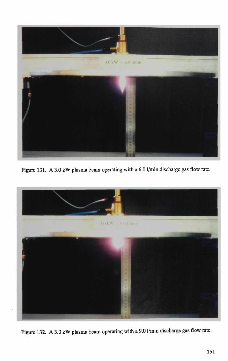
i.OkW
Figure 131. A 3.0 k W plasma beam operating with a 6.0 l/min discharge gas flow rate.
Figure 132. A 3.0 k W plasma beam operating with a 9.0 l/min discharge gas flow rate.
151
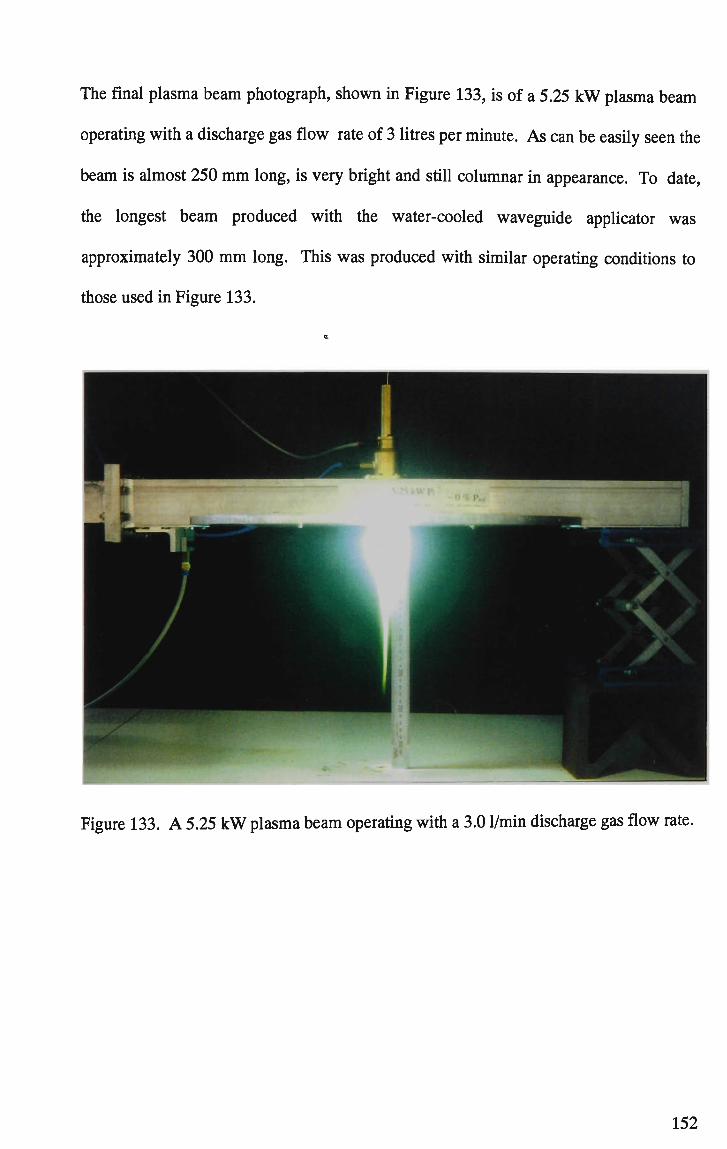
The final plasma beam photograph, shown in Figure 133, is of a 5.25 k W plasma beam
operating with a discharge gas flow rate of 3 litres per minute. As can be easily seen the
beam is almost 250 mm long, is very bright and still columnar in appearance. To date,
the longest beam produced with the water-cooled waveguide applicator was
approximately 300 mm long. This was produced with similar operating conditions to
those used in Figure 133.
Figure 133. A 5.25 k W plasma beam operating with a 3.0 l/min discharge gas flow rate.
152

4.10 Heat Capacity of the Plasma Beam.
The impetus for using indirect methods to determine the relative temperature was that
the plasma was too hot for conventional thermometry techniques. The use of
thermocouples was abandoned because it was easy to melt the platinum-
platinum/rhodium from which they are constructed. Optical pyrornetry of the plasma
was not feasible as the plasma was essentially transparent at the wavelength used by the
available equipment.
Two separate experiments were performed to qualitatively determine how the heat
capacity of the plasma beam varied with ionisation chamber diameter, discharge gas
flow rate and microwave power. The first used the non-cooled version of the waveguide
applicator and relied on the temperature rise of a known mass of water. The second
utilised the water-cooled applicator and used the temperature rise of a metal plate
immersed in the plasma. Factors that could influence the temperature rise of the water,
such as gas circulation patterns and turbulence, were not controlled and were assumed to
be the same for both experiments. The importance of knowing the heat capacity of the
beam becomes evident when materials welding and joining applications are considered.
To optimise the welding process, it is necessary to know in advance the heat input into
the weld pool and thus, the heat that can be extracted from the "welding torch". The
data for this section was generated collaboratively with another researcher [53] but was
analysed independently to provide the results given here. The experimental arrangement
used to determine the heat capacity of the plasma beam is shown in Figure 134 and the
power supply used was the non-commercial unit.
153

Water Filled Test Tube
Incident Microwaves
Discharge Gas Inlet
Figure 134. Experimental arrangement used to determine the heat capacity of the
plasma beam.
To determine the heat capacity it was necessary to monitor and record the incident
microwave power, the reflected microwave power, the initial and final temperature of
the water, the mass of water and the discharge gas flow rate. Two different diameter
alumina ionisation chambers were used. These had an I.D. and O.D. of 4 x 6.1 mm and
5 x 7.2 mm respectively. The distance x was not varied during the course of
experimentation to ensure uniformity of experimental conditions. An estimate of the
heat capacity of the plasma was then calculated from
Q = mciTf-Ti)
(W)
154

where:
m = mass of water (kg)
c = heat capacity of water (4184 J/kg.K)
Tf = final water temperature (K)
Tt = initial water temperature (K)
t = time interval (s)
160
140
^120 1
& 100 H
§ 80 u
5 60
s 03 40
20 0
I.D. x O.D. = 4x6.1 m m
N
5 litres/minute 10 litres/minute
15 litres/minute * 20 litres/minute
1.25 1.5 1.75 2 Microwave Power (kW)
2.25 2.5
Figure 135. Heat transfer data for the non-cooled plasma (small ionisation chamber).
The heat transfer results are given in Figure 135 and Figure 136. Both Figures show the
general trend of increasing heat capacity of the plasma beam with increasing power as
would be expected. Both ionisation chambers have a similar internal diameter and as
such, the results would be expected to be similar. This is born out by the results. What
is not clear from the results is whether there is a trend of increasing heat transfer from
the plasma beam with increasing flow rate. It is more likely that the heat transferred is
not a linear function of increasing flow rate but involves a turning point, i.e. a point in
155

the gas flow rate beyond which the available heat from the plasma starts to decrease.
This topic is investigated further in Chapter 5.
^
£ hi .<u CM ifi S OS u H
s a
180
160
140
120
100
80
60
40
20
0
I.D. x O.D. = 5 x 7.2 m m
x
'+- 5 litres/minute —"~ 10 litres/minute 4 15 litres/minute "*- 20 litres/minute
1.25 1.5 1.75 2 2.25 2.5 Microwave Power (kW)
2.75
Figure 136. Heat transfer data for the non-cooled plasma (large ionisation chamber).
The second experiment, to determine the relative heat capacity of the plasma beam, is
similar to that shown schematically in Figure 134 except the test-tube is replaced by a
section of 3 mm plate steel and the commercial power supply and water-cooled
applicator used. The experiment involved immersing a metal plate into the plasma for a
known period. A thermocouple was mounted on the rear of the plate to allow for
temperature determination and the standoff distance, x, was computer controlled. The
microwave power was set at 2.75 kW and the standoff distance of the metal plate at 6
mm where the standoff distance is the distance of the plate from the plasma exit nozzle.
The results shown in Figure 137 represent the heat capacity of the plasma beam as a
function of discharge gas flow rate and the results in Figure 138, a fixed microwave
power and discharge gas flow rate of 3 kW and 4 litres/minute respectively.
156

1300 Y 1200 4
£ 1100 i ~ 1000-3 900-U 800:; a 700-
E cu H
1
600: 500: 4oo-300-200 100 1 0
H-KH
2.75 kW Plasma, 6 m m Standoff Distance.
4 6 8 10 Discharge Gas Flow Rate (litres per minute)
12
Figure 137. Relative plasma beam temperature as a function of discharge gas flow rate.
The data shown in Figure 138 is consistent with that shown in Figure 135 and Figure
136 inasmuch as the beam temperature is not a linear function of discharge gas flow
rate. This consistency between data sets means that both the non-cooled and cooled
applicators behave in a similar manner. The maximum heat extracted from a 2.75 kW
beam with a 6 mm standoff distance occurred for a gas flow rate of 9 litres/minute. The
results shown in Figure 138 reveal that the beam temperature, or more correctly the heat
capacity of the beam, decreases with distance from the exit nozzle. This is totally as
expected since as the standoff distance is increased, so too is the distance from the
excitation source for the plasma. Even though Figure 137 and Figure 138 show relative
beam temperature, it should strictly be the heat capacity of the beam since the
temperature of the plasma is not a well defined quantity as the thermal equilibrium
status is not known. These experiments provide a direct measure of the heat that can be
extracted from the plasma beam, an important quantity in terms of use as a heating or
welding tool.
157

920
/^s i-r r _ -
5U
1 ee M
o» a E s H 5! •43 88
cu X
•
900 t
""
8 8 0 -
860"
8 4 0 -
T
8 2 0 -
800 -I ' 1 ' 1 ' 1 ' ' !
1 3 5 7 9 11 Plate Standoff Distance (mm)
Figure 138. Relative plasma beam temperature as a function of plate standoff distance.
4.11 Plasma B e a m Pressure.
Another important characteristic of the plasma beam, in terms of applicability as a
welding tool, is the pressure the beam exerts on the workpiece. A high beam pressure
will essentially eject the molten metal as the beam melts the workpiece instead of
allowing it to cool in situ. This results in a cutting action instead of the desired welding
or fusing action. Figure 139 shows schematically the experimental arrangement used to
determine the plasma beam pressure. The face of the water-cooled copper block was
positioned 0.3 mm away from the exit nozzle. This dimension is represented by x in
Figure 139. The copper block had a fine Pitot hole, which was connected to a
differential manometer from which the pressure could be read. The differential pressure
was measured with respect to atmospheric pressure.
3 k W Plasma, 4 l/min Gas Flow Rate
158

Water Cooled Copper Block
PitotHole Output to Differential Manometer
Coolant Out •
Incident Microwaves
Discharge Gas Inlet
Figure 139. Experimental arrangement used to determine plasma pressure.
Figure 140 gives the relative plasma pressure as a function of discharge gas flow rate for
various plasma beam powers. As can be seen, each curve is parabolic in nature and is
qualitatively explained by Bernoulli's principle. A full description can be found in Fox
and McDonald [54] but put simply, the density of the gas, or plasma, changes with
temperature and the pressure exerted by the gas is a function of the square of the mass
flow rate per unit area of the gas. Theoretically, if the pressure and mass flow rate are
known, then the temperature of the gas can be calculated from the density. This works
well for an idealised Pitot tube but was not applicable to the above experimental
arrangement.
159

1050
+- No Plasma -•- 2.5 kW • 3.25 kW • 3.5 kW
2.75 kW 4.0 kW
3.0 kW
08 X
08
I
1000-
950
900-
850
800
750
700 H h -I 1 1 y-
2.5 3.5 4.5 5.5 6.5 7.5 8.5 9.5 10.5
Discharge Gas Flow Rate (litres per minute)
Figure 140. Relative plasma pressure as a function of discharge gas flow rate.
Figure 141 is the data from Figure 140 presented in a different form, namely, the
relative plasma pressure as a function of microwave power. From this Figure, it is quite
evident that the plasma beam pressure increases with increasing plasma beam power,
which corresponds to an increasing temperature. The base pressure was 760 mm of
mercury and the maximum pressure obtained was 999 mm of mercury. This
corresponds to an increase of approximately 30 %, which is quite significant in terms of
the pressure exerted on the molten weld pool. Due to technical difficulties, data
corresponding to a microwave power of 3.25 kW and discharge gas flow rates from 7
through 10 litres per minute was not obtained. This was also the case for a power of 3.5
kW and a flow rate of 10 litres per minute.
The results presented in Figure 140 and Figure 141 are important from a welding and
joining applications standpoint. The pressure the plasma exerts on the molten weld pool
is a critical variable of which knowledge is necessary to perform good quality welds.
160

u 08 rO
s 1 a 9 88
E
a
1050
1000
950
900 -
850 -
800 -
750 -
700
-«— 3 litres/minute
*- 6 litres/minute -»— 9 litres/minute
4 litres/minute 7 litres/minute 10 litres/minute
*- 5 litres/minute *- 8 litres/minute
2.25 2.75 3.25 3.75 Microwave Power (kW)
4.25
Figure 141. Relative plasma pressure as a function of microwave power.
4.12 Conclusion.
This chapter has dealt with the characterisation of the plasma/applicator system through
determination of the electrical and physical properties of the plasma. In Section 4.3,
VSWR measurements on the non-cooled waveguide applicator revealed that there was a
small change in load impedance phase with power and a steady change in the load
impedance magnitude and phase with increasing sliding short-load distance. Also
revealed by the VSWR measurements was the existence of a resonance condition
whereby the load impedance was matched to that of the source. This occurred for a
sliding short-load distance of approximately 80 mm. Analysis of the resonance
condition for the cases with and without a plasma revealed that the quality factor of the
cavity, Q, was greater in the absence of the plasma. The broadening of the resonance
peak by the plasma is advantageous when constructing an applicator since the cavity
dimensions are not as critical and the applicator is less sensitive to drifts in the driving
frequency. The gradient of the VSWR linear regression line as a function of microwave
161
power was opposite on either side of the resonant position. Starting with the sliding
short-load distance less than the resonance length, as the sliding short was moved closer
to the resonance position, the slope of the regression line becomes less positive and the
magnitude of the VSWR was reduced for a given power level. Once the resonance
position has been passed however, the slope of the regression line took on ever larger
negative values and the VSWR for a given power increased. The positioning of external
chokes on the applicator to reduce microwave leakage had no effect on the recorded
VSWR.
Measurements of the electrical impedance of the plasma beam enabled a simple
electrical circuit model of the plasma to be developed (Section 4.4). The plasma
contained an inductive component that remained essentially unchanged with short
circuit stub position and this component was interpreted as the inductive component of
the plasma column. Modelling the plasma column as a perfectly conducting wire
stretched across the broadwall of the waveguide gave excellent agreement between the
experimentally and theoretically determined value for the inductive susceptance of the
plasma beam at resonance. Measurements of the electrical impedance of the plasma as a
function of sliding short-load distance revealed that the real component of the
impedance had a sharp maximum around resonance whilst the imaginary component of
the plasma impedance fell to zero at resonance (Section 4.5). Neither the real nor the
imaginary part of the plasma impedance varied much with microwave power over the
range 0.5 through to 1.5 kW though both these properties did increase marginally with
discharge gas flow rate.
162

Section 4.6 dealt with V S W R measurements on the water-cooled waveguide applicator.
The VSWR decreased for microwave powers of 0.75 through 5 kW and discharge gas
flow rates of 1 through 10 litres per minute. This is in agreement with the VSWR
characteristics of the non-cooled applicator. In Section 4.7 it was shown that the real
component of the plasma impedance increased with discharge gas flow rate as well as
microwave power whilst the imaginary component decreased with increasing gas flow
rate and microwave power. There was an important difference between the imaginary
components for the non-cooled and cooled applicators. Specifically, the plasma beam
produced by the non-cooled applicator contained an inductive component whereas the
cooled applicator produced a beam with a capacitive reactance. It is suggested that this
is the result of the physical arrangement of the cooling system having an electrical
resemblance to a cylindrical capacitor. When compared to the literature, there was little
agreement between the plasma impedance for a plasma generated by either the non-
cooled or the water-cooled applicator (Section 4.8). This is due to the use of different
discharge gases as well as the different physical arrangements of the applicators. Both
impedances reported in the literature had a capacitive reactance as did the water-cooled
applicator as previously mentioned.
Section 4.9 showed that the overall plasma beam length increased with increasing
microwave power as did the central core of the beam. As the discharge gas flow rate
was increased for a given power, the overall beam length decreased whilst the core
length remained essentially static. The heat capacity of the beam, as discussed in
Section 4.10, increased with increasing power as would be expected. However, the
relative temperature of the beam as a function of discharge gas flow rate had a concave
downward structure with a maxima beam temperature corresponding to a discharge gas
163

flow rate of 9 litres per minute. For a given microwave power and discharge gas flow
rate the plasma temperature decreases with increasing standoff distance as would be
expected. In Section 4.11, the pressure the plasma beam exerted on the workpiece was
measured using a differential pressure transducer. Results indicated that the pressure
exerted by the beam increased with increasing discharge gas flow rate and increasing
microwave power.
Welding has been an accepted method for joining disparate samples for many years and
techniques have been optimised through trial and error methods. Some aspects of
welding are still an art since many processes are not yet well understood. As discussion
of the use of a microwave induced plasma beam as a welding tool is largely absent from
the literature, much work at characterising the beam's properties as a function of
external parameters is necessary. For example, the beam temperature and the pressure
the plasma exerts on the molten weld pool are critical variables, prior knowledge of
which is necessary to perform good quality welds.
164

CHAPTER 5. PLASMA TEMPERATURE DETERMINATION BY LASER
SCATTERING TECHNIQUES.
5.1 Introduction.
This chapter deals with the determination of the plasma temperature through laser
scattering techniques. Scattering of photons by particles small compared to the
wavelength of light is known as Rayleigh scattering and is a useful diagnostic tool for
measuring particle densities [55]. The intensity of the Rayleigh scattered signal is
directly proportional to the number density of scattering centres, i.e. argon ions and
atoms in the present case, and provides a measure of the number of scattering centres in
the scattering volume. The temperature of the plasma can then be determined from the
ideal gas law, PV=nRT. Where P, V, n, R and T are pressure, volume, number of atoms,
universal gas constant and the temperature respectively. Boyle's Law for a perfect gas is
a valid approximation for Rayleigh measurements below about 10000 K since the
population of the neutral argon ground state is more that 99% of the total heavy particle
population. From the ideal gas law, for a given scattering volume at fixed pressure, a
rise in temperature corresponds to a decrease in the number of scattering centres
contained within the scattering volume. The temperature of the heavy particles in the
plasma can then be calculated from knowledge of the number density of scattering
centres in argon at room temperature and pressure. This section describes the use of
Rayleigh scattered Nd:YAG laser light to determine the particle density, and hence
heavy particle temperature, of an argon based microwave induced plasma beam
operating between 1 and 5 kW.
165
5.2 Temperature Determination.
The experimental arrangement is shown schematically in Figure 142 [56]. A frequency
doubled, pulsed Nd:YAG laser was used as the laser source. Pulse duration and
frequency were 6 ns and 20 Hz respectively. The output laser wavelength was 532 nm
and the maximum pulse energy available at this wavelength was 320 mJ. The laser
beam was brought to focus, at the scattering site, at 90° to the scattering-collection
optics optical axis and within the focal plane of these optics. The scattered signal was
collected by an ARC monochromator and measured using a Princeton Instruments Inc
image intensified charge coupled detector (ICCD), model 576G/RBE. The ICCD array
was 578 pixels wide and the spectral difference between adjacent pixels was 0.059 nm.
Vertically, the pixel separation represents 0.022 mm at the laser focus. The entire
optical apparatus, including laser and collection optics, was mounted on an XYZ table
allowing the scattering site to be driven to any point within the plasma beam.
Using software control, the ICCD was configured for use in "spatial" mode. Spatial
mode gives a spatially resolved image for a vertical slice through the scattering site by
binning the appropriate horizontal pixels. In this mode the vertical profile of the laser
beam was evident as was the plasma and any reflected laser light. The width of the slice
through the scattering site was about 0.1 mm and was dictated by the width of the
vertical slit at the monochromator input. The collection optics axis was centred on the
plasma beam by scanning the beam across the scattering site, firstly in the x and then in
the y direction, and finding the position corresponding to a maximum scattered signal.
The beam centring was performed as close as possible to the nozzle where the plasma is
most uniform.
166

A/2 Plate Focussing lens
Mirror /£— £ |i Scattering Site
Nd:YAG Laser
Figure 142. Schematic diagram of laser scattering experimental apparatus.
After leaving the laser, the beam passes through expansion optics and a half wave plate.
The half wave plate allows the intensity of beam to be adjusted whilst maintaining full
power output from the laser. The laser is most stable when operated at full power. The
laser output from the Brewster plate is plane polarised with the electric field vector
oriented in the z direction. This results in isotropic scattering in the x-y plane and
minimises, in conjunction with the polarising plate in the collection optics path,
unwanted radiation from entering the detector. The diaphragms or apertures situated
after the focussing lens are used to minimise stray light from entering the collection
optics. Finally, the laser beam is brought to focus in the plasma before continuing to a
conical beam dump. The plasma beam is parallel to the z axis and the laser beam
interacts with the plasma orthogonal to this axis in the x direction. The Rayleigh
scattered signal is viewed in the y direction.
167

The entire experimental apparatus was enclosed in light absorbent curtaining to further
reduce stray light. The level of stray light could be checked by determining the
Rayleigh scattered signal for both room temperature argon and helium. The helium
signal is expected to be small compared to that from argon since their Rayleigh cross
sections, OAr:ote, are in the ratio 66:1 [57]. Measurements of the Ar.He Rayleigh
scattered signal revealed that the level of stray light was consistently found to be of
order of 0.6 % of the scattered signal from room temperature argon. At this level, the
stray light contribution to the scattered signal is sufficiently small that it can be ignored.
However, since the Rayleigh scattered signal decreases with increasing temperature, this
stray light can represent a background signal amounting to 25 % of the true signal at an
argon gas temperature of 8500 K.
870 820-; 770-
^720
1 670 §620
J* 5 7 ° "" ^ 5 2 0 " | 470 -; g 420 -3 370 -m 320 -
270 220 1 170 0
Room Temperature Argon
50 100 150 200
Pixel # 250 300 350 400
Figure 143. Rayleigh scattered signal for room temperature argon.
168

210
0 50 100 150 200 250 300 350 400
Pixel #
Figure 144. Rayleigh scattered signal for a 5 kW argon plasma beam.
The data presented in the first section of this chapter (up to Figure 162) represents
measurements nominally made "on-axis" of the plasma beam. As shown later in this
chapter, errors in positioning the laser beam "on-axis" can lead to errors of between
1000 and 2000 K in the measured temperatures. The data presented in Figure 143 and
Figure 144 was collected for 100 accumulations, 25 seconds, and is typical of the laser
scattering data collected. Figure 143 gives the intensity of the Rayleigh scattered signal
as a function of CCD pixel number for a room temperature argon beam and Figure 144,
for a 4 litre per minute 5 kW argon plasma beam. After integrating the area under each
curve, the temperature is then derived by taking the ratio of these areas and multiplying
the resultant by the room temperature, in Kelvin. For the above case, this corresponds
to a temperature of approximately 6000 K.
Figure 145 gives the plasma temperature as a function of microwave power for z = 2
mm and a discharge gas flow rate of 5 litres per minute. The increase in the size of the
169
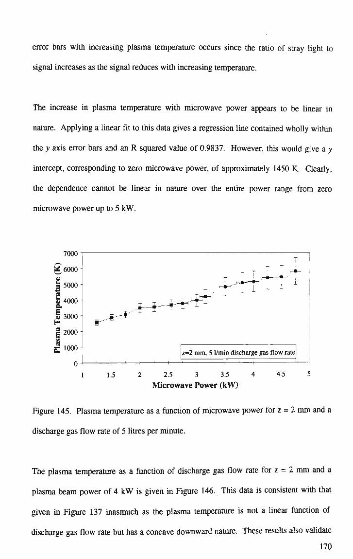
error bars with increasing plasma temperature occurs since the ratio of stray light to
signal increases as the signal reduces with increasing temperature.
The increase in plasma temperature with microwave power appears to be linear in
nature. Applying a linear fit to this data gives a regression line contained wholly within
the y axis error bars and an R squared value of 0.9837. However, this would give a y
intercept, corresponding to zero microwave power, of approximately 1450 K. Clearly,
the dependence cannot be linear in nature over the entire power range from zero
microwave power up to 5 kW.
7000
rl 6000
5000 2
i » 4000 a § 3000 H | 2000
a K IOOO
t r ^
1.5
1
z=2 mm, 5 l/min discharge gas flow rate
2.5 3 3.5
Microwave Power (kW) 4.5
Figure 145. Plasma temperature as a function of microwave power for z = 2 m m and a
discharge gas flow rate of 5 litres per minute.
The plasma temperature as a function of discharge gas flow rate for z = 2 m m and a
plasma beam power of 4 kW is given in Figure 146. This data is consistent with that
given in Figure 137 inasmuch as the plasma temperature is not a linear function of
discharge gas flow rate but has a concave downward nature. These results also validate
170
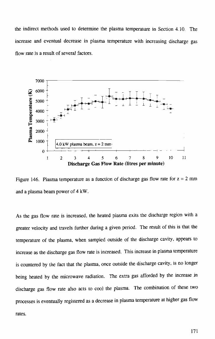
the indirect methods used to determine the plasma temperature in Section 4.10. The
increase and eventual decrease in plasma temperature with increasing discharge gas
flow rate is a result of several factors.
7000
o
4.0 kW plasma beam, z = 2 mm
1 2 3 4 5 6 7 8 9 10
Discharge Gas Flow Rate (litres per minute) ll
Figure 146. Plasma temperature as a function of discharge gas flow rate for z = 2 m m
and a plasma beam power of 4 kW.
As the gas flow rate is increased, the heated plasma exits the discharge region with a
greater velocity and travels further during a given period. The result of this is that the
temperature of the plasma, when sampled outside of the discharge cavity, appears to
increase as the discharge gas flow rate is increased. This increase in plasma temperature
is countered by the fact that the plasma, once outside the discharge cavity, is no longer
being heated by the microwave radiation. The extra gas afforded by the increase in
discharge gas flow rate also acts to cool the plasma. The combination of these two
processes is eventually registered as a decrease in plasma temperature at higher gas flow
rates.
171

a ^ r
2 a
I 88
E S
3 4500
4000 1
3500
3000
2500
2000
1500
1000
500
0
Hi
5 k W plasma beam, 4 l/min discharge gas flow rate
0 10 20 30 40 50 60 70 80 Height from Nozzle ( m m )
90 100 110
Figure 147. Plasma temperature as a function of distance from nozzle for a 5 k W , 4 litre
per minute plasma beam.
The plasma temperature as a function of distance from the exit nozzle for a 5 k W , 4 litre
per minute plasma beam is given in Figure 147. The scattering region was aligned with
the centre of the plasma beam and measurements taken at various distances along the
length of the plasma beam. Care was taken to ensure the scattering region was in the
centre of the plasma beam along its complete length, approximately 100 m m . As would
be expected, the plasma temperature decreases with increasing distance from the
excitation source. This is consistent with the findings of the heat capacity experiments
performed in Section 4.10 and the findings shown in Figure 146. This is important for
application to welding since they quantitatively describe the effects of two major
welding variables, gas flow rate and standoff distance. There is however a difference
between the data given in Figure 145 and that in Figure 147. Specifically, the
temperature shown in Figure 147 is approximately 2500 K less than that in Figure 145
172

for a similar discharge gas flow rate and plasma beam power. This is because the two
experiments were performed with different coolant flow rates.
The effect of coolant flow rate on plasma temperature is shown graphically in Figure
148. The increase in plasma temperature with decreasing coolant flow rate is because of
increased "ablation" of the inner surface of the ionisation chamber. The hotter the inner
surface the greater the number of electrons ejected into the plasma by thermionic
emission. These electrons are accelerated by the electric field of the microwaves and
contribute to increasing the plasma temperature through collisional processes. Also, as
the inner surface of the ionisation chamber is hotter with a decreased coolant flow rate,
less energy is taken from the plasma through conduction. Note that the curve shown in
Figure 148 appears to have a step like nature. This result is unexpected and the step in
plasma temperature may be the result of a change in coupling between the microwaves
and the plasma as the coolant flow rate is varied.
7000
6000-
5000-r-j - r ^
9 g 4000 u a S 3000 H 2 2000 | 5 1000
0
4 k W plasma beam, 3 l/min discharge gas flow rate
0.01 0.015 0.02 0.025 0.03
Coolant Flow Rate (litres per second) 0.035
Figure 148. Plasma temperature as a function of coolant gas flow rate for a 4.0 k W
argon plasma beam.
173

The applicator coolant temperature as a function of microwave power is shown in
Figure 149, and as a function of coolant flow rate in Figure 150. The curves presented
in these two Figures are consistent with expectations. That is, the coolant temperature
increases with increasing microwave power and decreases with increasing coolant flow
rate. The increase in coolant temperature with microwave power is principally due to
increased conduction of heat through the ceramic ionisation chamber associated with
increasing plasma temperature. Direct heating of the coolant by the microwaves is
comparatively insignificant since the annulus of coolant is 0.5 mm thick.
330
g> 320
2 « 315 ay | 310
Z 305 4 300 5 U 295
290
I
• i' a
T --
i i i i^-iy
5 l/min discharge gas flow rate
1.5 2 2.5 3 3.5 4
Microwave Power (kW) 4.5
Figure 149. Applicator coolant temperature as a function of microwave power for a
coolant flow rate of 0.01875 litres per second and a discharge gas flow rate of 5 litres
per minute.
174

s • r
2 cu
i ay
H e C8
335
330-
325 -
320 -
315 -
U 3 1 0 "
305
i
4 k W plasma beam, 3 l/min discharge gas flow ratej
0.01 0.015 0.02 0.025 0.03
Coolant Flow Rate (litres per second) 0.035
Figure 150. Applicator coolant temperature as a function of coolant flow rate for a 4
k W , 3 litre per minute plasma beam.
180
^ 1 6 0 "
E B 140 -|l20f
3 ioo
ay tt
80 1
60
40
20 1
0
0.01
rl^ ^i^k
"K ^
4 k W plasma beam, 3 l/min discharge gas flow rate
> *
0.015 0.02 0.025 0.03
Coolant Flow Rate (litres per second)
0.035
Figure 151. Plasma beam length as a function of coolant flow rate for a 4 k W , 3 litre
per minute plasma beam.
175

Figure 151 gives the plasma beam length as a function of coolant flow rate for a 4 k W , 3
litre per minute plasma beam. As can be readily seen from this graph, the maximum
beam length occurs for a coolant flow rate of approximately 0.02 litres per second. The
form of this curve is a result of a change in coupling of the microwaves to the plasma
with changing coolant flow rate. The fact that the ability of the microwave power to
couple with the plasma is dependent upon the flow characteristics of the coolant fluid is
important since it shows that thermionic emission of electrons from the hot ionisation
chamber is an important process in maintaining the plasma discharge. This is consistent
with the data given in Table 7 that showed that it was not possible to spontaneously
generate a plasma in a quartz ionisation chamber since this tube did not heat when
placed in the microwave field.
Figure 152 and Figure 153 give the plasma temperature and plasma beam length as a
function of sliding short-load distance for a 3 kW, 5 litre per minute plasma beam
respectively. The plasma temperature remains fairly constant at 3000 K for the sliding
short-load distance between 176 and 184 mm. At a distance of 184 mm and above the
temperature is reduced to approximately 2500 K. This transition in temperature
corresponds to the location of the resonance position for the water-cooled cavity. The
resonance position can be easily seen in Figure 153 as this position corresponds to a
maxima in plasma beam length. This result supports the hypothesis that the step like
nature of the plasma temperature in Figure 148 is the result of a change in coupling of
the microwaves with the plasma as the coolant flow rate is varied.
176

3500
£ 3000 1
j| 2500 88
|3 2000"
1 1500 H | 1000-
ei S 500-
0
i — * - - i-p-r^"
3 k W plasma beam, 5 l/min discharge gas flow rate, 3mm height
174 176 178 180 182 184 186
Sliding Short-Load Distance (mm) 188
Figure 152. Plasma temperature as a function of sliding short-load distance for a 3 kW,
5 litre per minute plasma beam.
no 100 1
i 90 5- 80-
f 70~ j 60 a 50 CQ
* 40 I 30 J 20-Qr
io -0
174
ir \--mr\
U-f
3 k W plasma beam, 5 l/min discharge gas flow rate
176 178 180 182 184 186
Sliding Short-Load Distance (mm) 188
Figure 153. Plasma beam length as a function of sliding short-load distance for a 3 kW,
5 litre per minute plasma beam.
177

7000
S 6000 -
0
-*~2.5kW
-*~4.5kW
3.0 kW
5.0 kW 3.5 kW
Height = 2 m m above nozzle
4.0 kW
4 5 6 7 8 9 Discharge Gas Flow Rate (litres per minute)
10
Figure 154. Plasma temperature as a function of discharge gas flow rate for various
argon plasma beam powers.
Figure 154 gives the plasma temperature as a function of discharge gas flow rate for
argon plasma beam of powers 2.5 through 5.0 kW in increments of 0.5 kW and for a
fixed standoff distance of 2 mm. For a given flow rate there is generally an increase in
temperature with increasing power whilst for a given power, the maximum temperature
occurs for a flow rate of between 5 and 8 litres per minute. Since steel melts at around
1800 K, any plasma beam power above 1.5 kW would be suitable for welding steel.
The plasma beam power used however would depend upon the speed and heat affected
zone that was acceptable for the weld being performed.
Figure 155 through Figure 161 gives the plasma temperature as a function of discharge
gas flow rate and various exit nozzle distances for an argon plasma beam of powers
1.5kW through 4.5 kW in increments of 0.5 kW. In each of these Figures, the
temperature of the beam does not vary much for a given discharge gas flow rate and a
standoff distance up to 5 mm away from the exit nozzle. At distances greater than 15
178

m m from the nozzle, the temperature is reduced sequentially with distance for a given
flow rate. In Figure 155, the temperature increases from around 2250 K up to 3250 K
for flow rates of 4 to 10 litres per minute and standoff distances up to about 10 mm.
The trend of increasing temperature is smooth with what appears to be a gradual
tapering off in temperature in the region above 3000 K. This same trend of a gradual
increase with a tapering off of temperatures towards higher gas flow rates occurs for
each of the Figures through to Figure 161. The results given in Figure 160 and Figure
161 show a reduced maximum temperature when compared to those given in Figure 158
and Figure 159. This is due to instrumentation failure prior to data collection. These
results are included however, because they show the temperature as a function of
discharge gas flow rate curves have the same form at these powers as at lower powers.
Q H • , • 1 • ! . 1 • 1 ' 1
4 5 6 7 8 9 10 Discharge Gas Flow Rate (litres per minute)
Figure 155. Plasma temperature as a function of discharge gas flow rate for a 1.5 kW
argon plasma beam.
179

Discharge Gas Flow Rate (litres per minute)
Figure 156. Plasma temperature as a function of discharge gas flow rate for a 2.0 k W
argon plasma beam.
1 mm "~•" 2 mm * 3 mm * 4 mm —*~~ 5 mm ~*~ 10 mm
15 mm ~~~~ 20 mm ~~~~ 30 mm 40 mm —6~ 50 mm
3 4 5 6 7 8 9 10
Discharge Gas Flow Rate (litres per minute)
Figure 157. Plasma temperature as a function of discharge gas flow rate for a 2.5 kW
argon plasma beam.
180
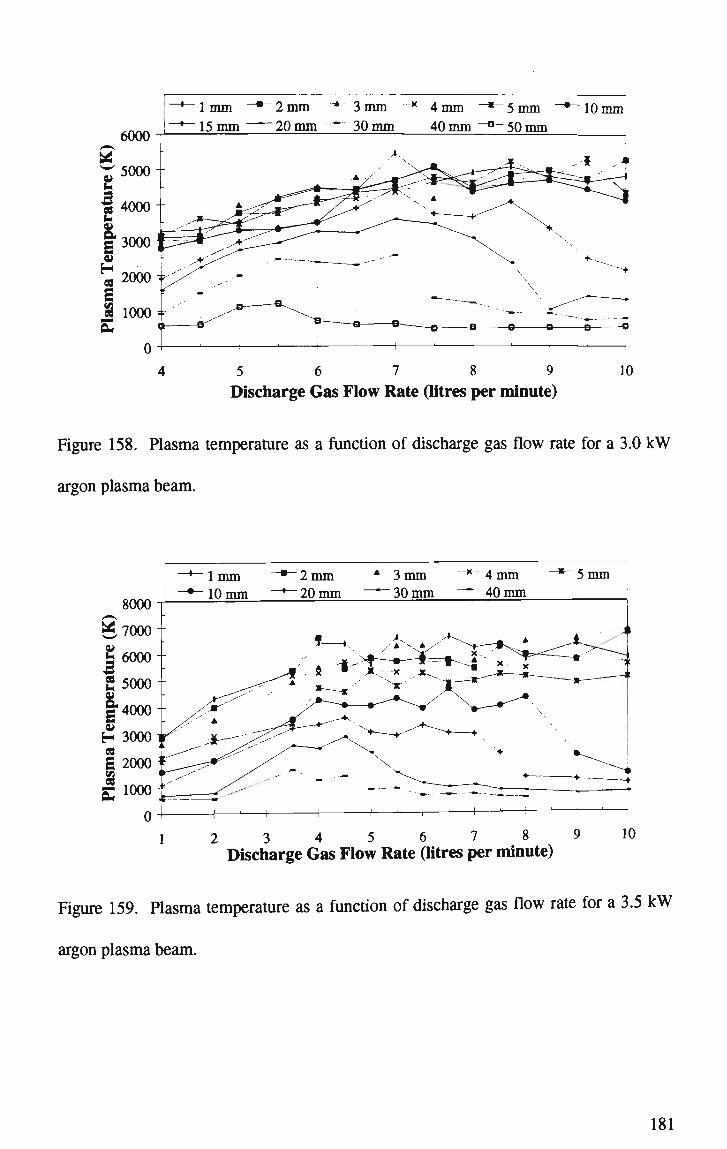
^-lmm -"-2mm ~* 3mm ~* 4mm -*-5mm ~*~10mm *— 15 mm ~~~~ 20 mm ~~~" 30 mm 40 mm ~&~ 50 mm
4 5 6 7 8 9 10 Discharge Gas Flow Rate (litres per minute)
Figure 158. Plasma temperature as a function of discharge gas flow rate for a 3.0 k W
argon plasma beam.
2 3 4 5 6 7 8 9 10 Discharge Gas Flow Rate (litres per minute)
Figure 159. Plasma temperature as a function of discharge gas flow rate for a 3.5 k W
argon plasma beam.

lmm —•"2mm "*" 3mm ^* 4mm -*-5mm ~•- 10mm
Discharge Gas Flow Rate (litres per minute)
Figure 160. Plasma temperature as a function of discharge gas flow rate for a 4.0 k W
argon plasma beam.
•-lmm -*~2mm * 3mm * 4mm ^"Smrn _#_10mm
Discharge Gas Flow Rate (litres per minute)
Figure 161. Plasma temperature as a function of discharge gas flow rate for a 4.5
argon plasma beam.

Figure 162 through to Figure 164 give the plasma temperature as a function of radial
distance for various microwave powers and discharge gas flow rates and at various
standoff distances. The plasma beam is about 3 mm wide at the exit nozzle and this is
reflected in these Figures by the rapid reduction in temperature with radial distance as
seen in the 0.5 and 1 mm standoff curves. This data suggests that errors in positioning
the laser beam "on-axis" can lead to errors of between 1000 and 2000 K in measured
temperatures. As the distance from the nozzle increases the surrounding air is heated by
the plasma and as a result the temperature falls away more slowly with radial distance.
The results given in Figure 163 and Figure 164 are for an identical plasma though the
data in Figure 163 was collected by sampling a cross section of the plasma in the x
direction whereas the data in Figure 164 has been sampled by scanning in the y
direction.
«r»N
5500
5000
4500
| 4000
g 3500
S, 3000
| 2500
« 2000
| 1500
gj 1000
500
0
"•-0.5 mm
-*—4mm -*^10mm * 20 mm "*—40 mm
5 kW plasma beam, 3 l/min discharge gas flow rate
-A . X
r" irK
I
1
V
X
X '.X
-r-
-3 - 2 - 1 0 1 Radial Distance ( m m )
Figure 162. Plasma temperature as a function of radial distance for a 5 k W , 3 litre per
minute plasma beam.
183

6000
tt 5000-
3 4000
2 1*3000
2 2000 £ 8 g; looo
L
•
-
•
1 1 mm
-+"3mm * 5 mm
~*~ 10 mm _*^20mm
-•- 40 mm 1 60mm
3 k W plasma beam, 5 l/min discharge gas flow rate • l^S.
x -
//
- 2 - 1 0 1 2 Radial Distance (mm)
Figure 163. Plasma temperature as a function of x-axis radial distance for a 3 kW, 5
litre per minute plasma beam
- 2 - 1 0 1 2 Radial Distance (mm)
Figure 164. Plasma temperature as a function of y-axis radial distance for a 3 kW, 5
litre per minute plasma beam.
184

The most obvious difference between these two sets of data is the maximum
temperature obtained for zero radial distance for the curves with a 1 through 10 mm
standoff distance. Clearly, there can be no difference as the plasma beam is identical.
In actuality, the temperatures shown are the same within experimental limits though the
error bars have been omitted from these graphs for reasons of clarity.
Figure 165 shows a contour map of plasma temperature as a function of y-axis radial
distance and distance from the nozzle for a 3 kW, 5 litre per minute plasma beam. This
graph was generated by applying a Gaussian fit to the data contained in Figure 164. The
correlation coefficient was greater than 0.975 in each case and the experimental data
along with the regression lines are given in Figure 166. Also shown on Figure 165 is an
outline of the visual plasma beam for comparison purposes. From this graph it can
deduced that the plasma is radially symmetric and decreases in temperature in a smooth
fashion away from the excitation source. Furthermore, even though the width of the
plasma does not vary appreciably over the length of the beam, the diameter of the hotter
core of the plasma beam does, tapering to zero at the 5 mm mark.
185
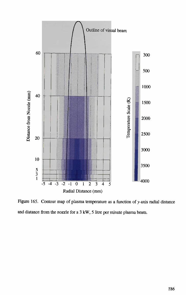
Outline of visual beam
e S •8 N &
e & o CO
a
300
500
1000
1500
2000
2500
3000
3500
-5 -4 -3 -2 - 1 0 1 2 3 4 5 4 0 0 °
Radial Distance (mm)
Figure 165. Contour map of plasma temperature as a function of y-axis radial distance
and distance from the nozzle for a 3 kW, 5 litre per minute plasma beam.
r-r
o CO p
S
186

4000
r~\
pm
ft B 2
E H cs E 8
3500
3000
2500
2000
1500
1000
500
1 m m Gaussian Fit 5 m m Gaussian Fit 10 m m Gaussian Fit 20 m m Gaussian Fit 60 m m Gaussian Fit
x 1 m m Experimental Data + 5 m m Experimental Data i
x o
10 m m Experimental Data 20 m m Experimental Data 60 m m Experimental Data
-5 - 2 - 1 0 1 2 Radial Distance ( m m )
Figure 166. Plasma temperature as a function of y-axis radial distance and distance
from the nozzle for a 3 kW, 5 litre per minute plasma beam.
Figure 167 through to Figure 171 give the plasma temperature as a function of x-axis
radial distance for various standoff distances and plasma beam powers. Again, error
bars have been purposefully omitted for reasons of clarity. These results show that, for
a given radial distance and standoff distance, the temperature of the plasma increases
with increasing microwave power. It should be noted here that, within experimental
limits, the curves for 4 and 5.75 kW in Figure 168 for example are the same. Note also
that the plasma temperature for each power level converges to the same value at a radial
distance of 3 mm. This distance places the sampling region outside of the plasma beam
and the temperature recorded is the ambient room air temperature. Since the sampling
region outside of the plasma beam does not contain argon, the temperatures recorded
will be in error. This is because the measurement procedure depends on the ideal gas
187

like behaviour of the discharge gas. To a first approximation though, these values are
reasonable. The same applies for each measurement taken on the fringe of the plasma
beam, i.e. essentially every figure from Figure 162 through to Figure 171. Note also that
as the standoff distance, or the distance from the nozzle, increases the temperature
gradient between the centre and the edge of the plasma beam decreases. This is due to
the thermalisation of the plasma beam with time after it leaves the excitation region
within the ionisation chamber.
0 0.5 1 1.5 2 2.5 3
Radial Distance ( m m )
Figure 167. Plasma temperature as a function of x-axis radial distance for z=l and 2
mm and various plasma beam powers.
188

7000
0.5 1 1.5 2 Radial Distance (mm)
2.5
Figure 168. Plasma temperature as a function of x-axis radial distance for z=5 m m and
various plasma beam powers.
tt
8000 T
7000
a 3 a ii
H
§ Sir
6000
5000
4000
3000
2000
1000
0.5 1 1.5 2
Radial Distance (mm)
2.5
Figure 169. Plasma temperature as a function of x-axis radial distance for z=10 m m and
various plasma beam powers.
189

7000
<-* 6000 tt
0.5 1 1.5 2 Radial Distance (mm)
2.5
Figure 170. Plasma temperature as a function of x-axis radial distance for z=20 m m and
various plasma beam powers.
4000
0.5 1 1.5 2
Radial Distance (mm)
Figure 171. Plasma temperature as a function of x-axis radial distance for z=40 m m and
various plasma beam powers.
190

5.3 Temperature Comparisons.
Cobine and Wilbur [4] give an estimation of the gas temperature of a plasma flame as
1870-3740 K though it is not clear from the text what frequency or power was used to
generate this data. The temperature was determined using buoyancy methods in which
the upward deflection of a horizontally directed flame was measured and the trajectory
determined. From this, an estimation of the temperature was made. The results of
Cobine and Wilbur are in good agreement with those in Chapter 5 as they fall well
within the gas temperature range generated by the water-cooled waveguide applicator.
Though this result is interesting, since neither the discharge gas, applicator type or
operating frequency are similar to those used above, it is difficult to say whether this
agreement is significant.
Direct comparison of the temperatures contained within Chapter 5 with those of Arata et
al [14] is difficult since the applicator of Arata is not a cavity but rather a coaxial design.
The same is true of the temperatures determined by Murayama [13]. Also the discharge
gas used by Arata was nitrogen, not argon. The temperatures determined by both Arata
and Murayama were not directly measured but determined from methods such as
electron density measurements and the Saha equation. Thus the temperatures were
derived with the assumption that the plasma was in a state of LTE. Acknowledging this,
it is possible however to look at the trends contained in the data and compare this to the
data obtained using Rayleigh scattering techniques. Murayama obtained the gas
temperature in the mantle of 200 and 400 W plasmas from measurements of the Doppler
broadening of the CaIlA,3934 Angstrom line, where calcium chloride was used to seed
the plasma. The values obtained were 4500±900 K and 4600±1000K respectively.
191

These two temperatures are within the range of temperatures determined using laser
scattering techniques though an order of magnitude more power was necessary to
achieve an identical temperature using the water-cooled waveguide applicator. If both
applicators produced similar plasmas then this discrepancy may have been due to the
probe element calcium. Calcium has a much lower ionisation potential than argon and
this would have had an impact on the temperature measured since the ionised calcium
would obtain energy from the oscillating electromagnetic field of the microwaves as
well as from collisional processes. From the work by Arata et al, Figure 41 is
qualitatively similar in form to Figure 147, that is, the temperature increases with axial
distance before decreasing for a given power and discharge gas flow rate. The
temperature measured by Arata is the electron temperature even though it is referred to
as the plasma temperature. The distinction is made between the electron temperature as
measured by Arata and Murayama and the gas temperature as measured by Murayama
and that measured using laser scattering since the electron temperature is generally
higher than the gas or heavy particle temperature. Strictly speaking, this is true only
when the plasma is not in LTE as happens in the majority of cases. Arata justifies the
assumption of LTE for nitrogen and air at atmospheric pressure from generally stated
arc plasma results.
The plasma temperatures as a function of microwave power, as given in Figure 42 and
Figure 145, are also qualitatively similar in form. The temperature discrepancy here is a
factor of two and both curves show the same linear dependence over the power regime
examined. Figure 43 and Figure 164 show the plasma temperature as a function of
radial distance. In both instances, the temperature profile as a function of radial distance
is qualitatively similar. Arata also examines the plasma temperature as a function of
192
discharge gas flow rate, Figure 44. Again, the form of this curve is qualitatively similar
to that of Figure 146. It should be stated here that although the discharge gas flow rates
used for this thesis were an order of magnitude smaller than those of Arata, the velocity
of the discharge gas was two orders of magnitude larger. This is due to the much
smaller effective cross section of the ionisation chamber as compared to the coaxial
applicator of Arata.
The fact that the plasma temperature dependence curves are similar for the two different
applicator types, as well as discharge gases, implies that after the plasma leaves the
excitation region it has no memory of how it was formed and thus decays in an identical
manner for any type of applicator. As the temperature measured by Arata was not the
gas temperature, again direct comparison cannot be made unless the thermodynamic
properties of the plasma are known. The literature has both cases in support of [13, 58]
and against [4, 59] LTE conditions existing in a microwave generated plasma. In
actuality, the LTE condition most likely varies both axially and radially along the
plasma beam as the plasma has had more time to thermalise the further from the exit
nozzle the temperature is measured.
193

5.4 Conclusion.
This chapter has dealt with the determination of the plasma temperature through laser
scattering techniques and has shown that the temperature recorded is a function of
microwave power, discharge gas flow rate, applicator coolant flow rate, height from the
plasma exit nozzle and the state of tuning of the applicator. More specifically, the
plasma temperature increased with increasing microwave power, decreased coolant flow
rate and decreased height from the nozzle. For a temperature of 8500 K, the error
associated with this measurement is of order 25%. This falls to less than 1 % for
temperatures in the 500 K region. This is the first time that laser scattering techniques
have been applied to a microwave generated plasma for the purposes of temperature
determination.
The maximum temperature recorded was 7200 K and corresponded to measurements
taken on a 5.75 kW argon plasma beam, 2 mm away from the plasma exit nozzle. At
these temperatures, the equilibrium composition of the argon plasma consists mainly of
excited neutrals with less than 0.01 % of singly ionised argon [60]. Two-dimensional
temperature scans through the plasma beam have shown that a line scan of plasma
temperature taken through the plasma at each standoff distance could be successfully
modelled by a Gaussian distribution. This was done at various distances from the exit
nozzle to produce a spectral map of the plasma showing temperature contours in 500 K
steps. The temperature gradient from the centre to the edge of the plasma beam
decreased with distance from the excitation source of the plasma due to thermalisation
of the plasma.
194
The ability of the microwaves to couple to the plasma depends on the flow rate of the
coolant through the applicator and manifests itself in a variation in plasma temperature
and plasma beam length. A higher coolant flow rate corresponded to a lower plasma
temperature for a given microwave power and a shorter plasma beam length. The terms
microwave power and plasma beam power are used interchangeably since it is assumed
that essentially all the microwave power goes into producing the plasma as losses to the
walls are negligible as is the level of reflected power.
Variation of the sliding short-load distance, or the tuning of the applicator, had little
effect on the plasma temperature on the near side of the resonance position. However,
after the resonance position was passed, the temperature of the plasma beam decreased
rapidly with distance. This attribute is mirrored in the effect of sliding short-load
distance on the plasma impedance tabulated in Table 10. The implication here is that
the plasma temperature is a function of the load presented to the microwave source,
which is in turn a function of the tuning of the system.
Temperatures determined by laser scattering techniques compared well with those
determined using spectroscopic techniques in terms of the trends of temperature
dependence as a function of external variables. The absolute values for the temperatures
however did not though they were of the same order of magnitude. This was principally
due to the measurement of different species by the two techniques. Specifically, laser
scattering measures the temperature of the heavy particles within the plasma (both ions
and neutrals) whereas the spectroscopic methods used generated an electron temperature
through measurement of the electron density. This involved the assumption of LTE
conditions existing within the plasma. Technically speaking, temperatures are
195

determined from density measurements using laser scattering techniques also and the
assumption is the plasma behaves as an ideal gas. As the discharge gas is argon, this
assumption is more valid than an assumption of LTE. The use of different discharge
gases and applicator configurations also contributed to the discrepancy between the
temperatures measured by the two techniques. The temperatures measured using laser
scattering techniques were in better agreement with the gas temperatures than the
electron temperatures reported in the literature indicating the plasma may not be in LTE.
The temperature measurements presented provide strong evidence that the plasma is not
in LTE. For example, Figure 165 shows the extent of the "visual beam" being
associated with measured gas temperatures ranging from 3000 K to below 500 K.
The characterisation given in this chapter of the plasma beam temperature with
microwave power, discharge gas flow rate, coolant flow rate, state of tuning and
standoff distance is important in the application of the plasma beam to welding since
fine control over the temperature of the beam as well as the heat input into the sample is
critical to overall weld strength and quality.
196
CHAPTER 6. APPLICATION OF THE PLASMA BEAM TO WELDING OF
SHEET STEEL.
6.1 Introduction.
As previously mentioned the goal of this thesis was to develop a microwave generated
plasma device that could produce a beam of plasma capable of welding sheet steel. To
that end, this Chapter describes the culmination of research efforts to attain that goal.
Also contained in this Chapter are a set of experiments that were used to develop an
analytical model of the plasma beam operating conditions necessary to achieve
maximum weld strength in 1 mm G550 uncoated cold rolled sheet steel [61]. The
microstructure of the welded steel is examined, as is the weld strength across the fusion
zone. Weld strength tests were performed to Australian Standard AS2205 (Transverse
butt tensile test) and hardness test to Australian Standard AS 1817 (Vickers hardness
test). All samples were autogenously butt-welded and analytical modelling was
performed using Response Surface Modelling (RSM). RSM was used to model the
dependent variable response using mathematical models which were then used to
predict new response values, determine optimal variable settings and to produce contour
plots. The model generated is not so much predictive but a multiple regression best fit
of the variables to the weld strength of the generated welds.
The microwave plasma beam parameters that have an impact on weld quality, as well as
the ability to weld, have been quantified in Chapters 4 and 5. These are plasma beam
temperature and beam pressure. The beam temperature is a function of microwave
power, discharge gas flow rate, the state of tuning of the applicator, standoff distance
and the ionisation chamber coolant flow rate. To optimise the quality of the weld being
197

performed, as much heat as possible needs to be used so as to allow increased welding
speeds. Faster welding speeds mean reduced heat input per unit length into the sample
which limits the size of the heat affected zone (HAZ). Beam pressure is also a function
of microwave power and discharge gas flow rate. The complex inter-relationship
between these variables and their impact on weld performance was the principal impetus
for determining the way each variable impacted on the beam properties in previous
chapters.
6.2 Results of welding trials.
In order to perform a successful weld it was necessary to first determine what
combination of microwave power, discharge gas flow rate and welding speed should be
used. A sample measuring 180 x 120 mm was clamped in the welding table and a
combination of the aforementioned variables chosen such that the sample would melt
with full penetration when passed below the plasma beam. For a microwave power of
3.1 kW, this corresponded to a gas flow rate of six litres per minute and a welding table
translation speed of approximately 150 mm per minute. This technique was easy and
relatively quick to perform. Firstly, the power and gas flow rate were chosen and then
the sample set in motion below the plasma beam. If a cutting action ensued the table
speed was increased incrementally until the desired melting action was achieved. The
single sample was then replaced by the two samples to be welded
To best simulate industrial conditions, sample preparation was kept to a minimum and
all samples were cut into blanks using shears. The samples were a uniform size, had
dimensions of 90 x 120 mm and were prepared from 1 mm thick, uncoated mild steel.
198
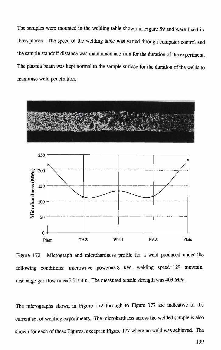
The samples were mounted in the welding table shown in Figure 59 and were fixed in
three places. The speed of the welding table was varied through computer control and
the sample standoff distance was maintained at 5 mm for the duration of the experiment.
The plasma beam was kept normal to the sample surface for the duration of the welds to
maximise weld penetration.
2 100
i § 50
0 ] 1 J 1 Plate H A Z Weld H A Z Plate
Figure 172. Micrograph and microhardness profile for a weld produced under the
following conditions: microwave power=2.8 kW, welding speed=129 rnm/min,
discharge gas flow rate=5.5 l/min. The measured tensile strength was 403 MPa.
The micrographs shown in Figure 172 through to Figure 177 are indicative of the
current set of welding experiments. The microhardness across the welded sample is also
shown for each of these Figures, except in Figure 177 where no weld was achieved. The
199

data points from left to centre correspond to the following regions; parent material or
plate, (HAZ) and fusion or weld zone. As can be clearly seen from all the welded
samples, the micro-hardness has a minimum in the region of the HAZ. The HAZ of the
welds generated using a microwave induced plasma beam can be further subdivided into
fine grained and coarse grained regions [62]. This fine grain structure is due to the
recrystallisation of the cold rolled ferrite grains at subcritical temperatures and
reaustenisation at supercritical temperatures, followed by transformation on cooling to
fine ferrite grains. The coarse grained HAZ is the result of significant growth of
austenite grains adjacent to the fusion boundary, followed by transformation to
relatively coarse ferrite on cooling. The slight increase in the microhardness of the
fusion zone is due to the formation of bainitic and/or martensitic ferrite on fast cooling
of the coarse columnar austenitic grains in the weld bead. These phases are relatively
hard and brittle. Welding reduces the strength and hardness in the weldment relative to
the cold rolled sheet. Under load conditions, the weld would fail in either the fine
grained HAZ or in the weld region itself. This is the principal impetus for reducing the
size of both the weld bead and the HAZ. This reduction can be achieved by increasing
both the welding speed and the plasma beam power. The shape and width of the HAZ
away from the fusion zone reflects the thermal profile of the weld.
200

Plate H A Z Weld H A Z Plate
Figure 173. Micrograph and microhardness profile for a weld produced under the
following conditions: microwave power=2.8 kW, welding speed=129 mm/min,
discharge gas flow rate=6.0 l/min. The measured tensile strength was 363 MPa.
Figure 172 and Figure 173 demonstrate the effect of discharge gas flow rate on the
measured tensile strength when all else is kept constant. The microstructure is similar
for both samples though there is a slightly higher number of larger grains Figure 173.
The existence of these larger grains leads to the reduction in weld strength.
Figure 174 shows good fusion but poor alignment. The misalignment is due to
limitations in the clamping mechanism of the welding table. This result is important
because it shows that tight fit-up tolerances are not necessary for the plasma beam
201
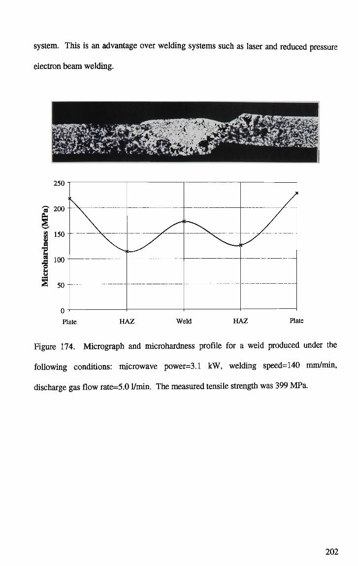
system. This is an advantage over welding systems such as laser and reduced pressure
electron beam welding.
250
| 150
I J 100
Plate
- r / r - r -
!
HAZ Weld HAZ Plate
Figure 174. Micrograph and microhardness profile for a weld produced under the
following conditions: microwave power=3.1 kW, welding speed--140 mm/min,
discharge gas flow rate=5.0 l/min. The measured tensile strength was 399 MPa.
202

Plate H A Z Weld H A Z Plate
Figure 175. Micrograph and microhardness profile for a weld produced under the
following conditions: microwave power=3.1 k W , welding speed--151 mm/min,
discharge gas flow rate=6.0 l/min. The measured tensile strength was 385 MPa.
Figure 175 and Figure 176 show the effect on the microstructure of varying the welding
speed for a given gas flow rate and microwave power. The microhardness and weld
strength is essentially the same for both samples even though there is a marked
difference in the grain structure at the fusion zone. This difference is due to the various
cooling rates of the H A Z and molten metal at different welding speeds. Note also the
existence of the inclusion in Figure 176. A s each welded sample is sectioned and
polished only once, it is not clear whether this inclusion is indicative of the entire weld
bead or an isolated occurrence. In all probability it is an isolated feature. Figure 177
shows a typical micrograph of a sample that has not been successfully welded because
203

the welding speed was too high or the microwave power too low. This sample was
welded, inasmuch as when it was removed from the welding table it did not separate
into the two blanks, even though there was no clearly defined fusion zone. Welds of
this nature could be easily broken by fatigue bending along the "weld bead".
Plate H A Z Weld H A Z Plate
Figure 176. Micrograph and microhardness profile for a weld produced under the
following conditions: microwave power=3.1 kW, welding speed=161 mm/min,
discharge gas flow rate=6.0 l/min. The measured tensile strength was 399 MPa.
204

Figure 177. Typical micrograph of an unsuccessful weld resulting from non optimum
welding conditions.
At a microwave power of 3.4 kW and welding speeds less than about 0.11 m/min, a
weld was not achieved due to the cutting action of the plasma beam. At speeds greater
than about 0.19 m/min, there was not enough time for the metal to reach melting point
before the beam had moved on. The opposite was true for the gas flow rate. A low gas
flow rate would not provide enough energy to weld whereas a high flow rate would cut
instead of weld. The increase in temperature provided by an increase in gas flow rate is
a double edged sword since not only does the temperature rise but so too does the
pressure exerted by the plasma on the weld pool. This can be readily seen in Figure
178. The plasma pressure increases as the square of the exit velocity of the plasma with
exit velocity being a function of temperature. At high enough velocities, the combined
effect of gravity and beam pressure overcomes the surface tension of the molten weld
pool and a cutting action is initiated. This is also true as the power is increased for a
given flow rate and weld speed, i.e. for a given flow rate, the exit velocity of the plasma
increases as the power is increased thereby exerting a greater pressure on the weld pool
or pressure transducer.
205

1100
S3- 'SlOOO ^ -8
£, -| 900 | -800 1 ^ 7 0 0 U 4)
| 1500 H £ 400
| | 300
| J 200 * K 100
0
Temperature " Pressure
4 6 8 10 Discharge Gas Flow Rate (litres per minute)
12
Figure 178. Effect of Plasma gas flow rate on plasma temperature and plasma pressure.
As discussed in Section 5.2, the levelling off of temperature with increasing flow rate in
Figure 178 is due to the cooling effect of the extra gas. The excited or heated gas loses
energy to the cool gas and with a limited amount of excitation energy, the overall
temperature of the plasma beam is reduced. Below about 9 l/min, there is enough
energy to excite the increase in gas afforded by the increase in flow rate.
0.5 m m
Figure 179. Micrograph of butt welded samples of different thickness' as used in
tailored blank technology.
206

Figure 179 shows the results of butt welding two samples of differing thickness', 0.5
mm and 1.0 mm. The microwave power used for welding these two samples was less
than that for two 1 mm samples being 2.1 kW. Welding of samples of different
thickness' is commonly used in the automotive industry and is referred to as tailored
blank technology. Tailored blank technology is designed to keep car component weight
down whilst still providing the key component strength by having thicker steel only in
the regions necessary. Examples of this are the hinge and lock regions of door
members.
Figure 180. Micrograph of 1 m m butt welded samples showing the effect of fit-up
misalignment.
In Figure 180, the results of welding two seriously misaligned samples are shown. As
previously mentioned, this misalignment is due to limitations in the clamping
mechanism of the welding table. Specifically, each sample is clamped in only three
places leading to sample buckling as the welding progresses. This micrograph is
included because it shows quite clearly the transformation of the grain structure
resulting from the welding process.
The weld strengths for the various combinations of microwave power, welding speed
and gas flow rate are tabulated in Table 11. Some combinations are duplicated for
207
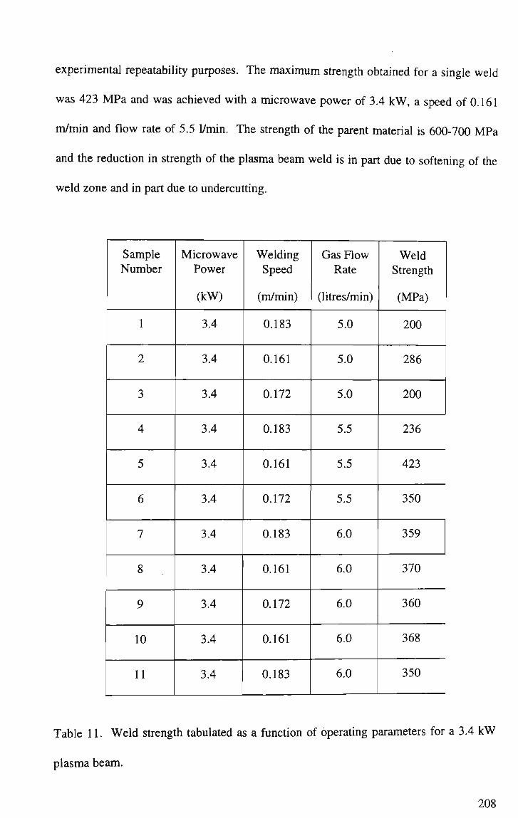
experimental repeatability purposes. The maximum strength obtained for a single weld
was 423 MPa and was achieved with a microwave power of 3.4 kW, a speed of 0.161
m/min and flow rate of 5.5 l/min. The strength of the parent material is 600-700 MPa
and the reduction in strength of the plasma beam weld is in part due to softening of the
weld zone and in part due to undercutting.
Sample Number
1
2
3
4
5
6
7
8
9
10
11
Microwave Power
(kW)
3.4
3.4
3.4
3.4
3.4
3.4
3.4
3.4
3.4
3.4
3.4
Welding Speed
(m/min)
0.183
0.161
0.172
0.183
0.161
0.172
0.183
0.161
0.172
0.161
0.183
Gas Flow Rate
(litres/min)
5.0
5.0
5.0
5.5
5.5
5.5
6.0
6.0
6.0
6.0
6.0
Weld Strength
(MPa)
200
286
200
236
423
350
359
370
360
368
350
Table 11. Weld strength tabulated as a function of operating parameters for a 3.4 k W
plasma beam.
208

Undercutting is inherent in butt-welded samples and leads to a reduction in sample
thickness along the weld line and hence a reduction in welded sample strength. The
weld strengths obtained are comparable with techniques such as mash seam welding;
however the welding speed is too low by almost an order of magnitude for practical
industrial applications. In order to increase the welding speed the energy density at the
weld pool needs to be increased by an order of magnitude. This could be achieved by
decreasing the exit nozzle orifice diameter from the current 3.2 mm down to 1 mm.
This is left as an exercise for future researchers.
6.3 Modelling of Welding Parameters.
Using the experimental results from Section 6.2, it was possible to analytically fit the
plasma beam operating conditions necessary to achieve maximum weld strength in 1
mm G550 uncoated cold rolled mild steel. Analytical regression analysis was
performed using a computer software package based on Response Surface Modelling
(RSM), with the dependent and independent variables used listed in Table 12.
Preliminary welding trials showed that for each power setting there was a unique
welding speed range that would result in acceptable welds. At the extremes of this
range, the results of the fit can be biased since there may not be enough heat for fusion
or too much resulting in a cutting action. This bias occurs since the software cannot
differentiate between too much power or too little power when a low or zero weld
strength is recorded. To overcome this problem, weld speeds were selected for the
various power settings that gave acceptable welds. This resulted in variable
combinations for the eleven welding experiments previously tabulated in Table 11. By
maintaining a constant microwave power of 3.4 kW and a constant butt pressure of 535
209
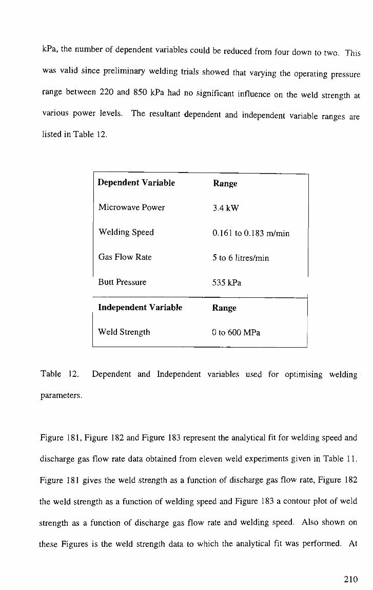
kPa, the number of dependent variables could be reduced from four down to two. This
was valid since preliminary welding trials showed that varying the operating pressure
range between 220 and 850 kPa had no significant influence on the weld strength at
various power levels. The resultant dependent and independent variable ranges are
listed in Table 12.
Dependent Variable
Microwave Power
Welding Speed
Gas Flow Rate
Butt Pressure
Independent Variable
Weld Strength
Range
3.4 k W
0.161 to 0.183 m/min
5 to 6 litres/min
535 kPa
Range
0 to 600 M P a
Table 12. Dependent and Independent variables used for optimising welding
parameters.
Figure 181, Figure 182 and Figure 183 represent the analytical fit for welding speed and
discharge gas flow rate data obtained from eleven weld experiments given in Table 11.
Figure 181 gives the weld strength as a function of discharge gas flow rate, Figure 182
the weld strength as a function of welding speed and Figure 183 a contour plot of weld
strength as a function of discharge gas flow rate and welding speed. Also shown on
these Figures is the weld strength data to which the analytical fit was performed. At
210

first glance the fit to the data given in Figure 181 seems poor and if it were not a
multiple regression then this would be the case. However, a multiple regression was
performed and as such there are compromises between the fit for each dependent
variable in order to obtain the best overall fit to the data.
-mu :
-
350: -
g 300:
^ 250 :
f : | 200: •_-2 150-
100:
50 :
i i i i i i i i i
y /
/ / / r
/
/
1 1 1 1 1 1 I 1 1
i i i ' I ' I I I I i ! i ; • i •
> ^ ^ ^ ^ " / ^
Welding Speed = 0.172 m/min
i i i • i r i i i i • i "• r • : • i • -
_, H
l : -:
-
--i
1
J
--
4.9 5.0 5.1 5.2 5.3 5.4 5.5 5.6 5.7 5.8 5.9 6.0 6.1
Gas Flow Rate (litres per minute)
Figure 181. Weld strength as a function of discharge gas flow rate for a microwave
power of 3.4 kW and a welding speed of 172 millimetres per minute.
From Figure 183 it can be seen that maximum weld strength of 400+ M P a was achieved
for a microwave power of 3.4 kW, for a flow rate of between 5.3 and 5.9 l/min, and a
welding speed of less than 0.166 m/min. This is not unexpected since a lower welding
speed was found to be necessary to generate a sound weld for the range of microwave
powers examined.
211

500
450-^
s f a Ir
-to-CC
2 "a>
400
350-:
3 00-
250-
200 Gas Flow Rate = 5.5 l/min
160 162 164 166 168 170 172 174 176 178 180 182 184
Welding Speed (millimetres per minute)
Figure 182. Weld strength as a function of welding speed for a microwave power of 3.4
k W and a discharge gas flow rate of 5.5 litres per minute.
-ta-
s o E 3 d oc IN
09
t
6.0
5.9
5.8
5.7
5.6
5.5
5.4
5.3
5.2
5.1
5.0
Weld Strength (MPa)
162 164 166 168 170 172 174 176 178 180 182
Welding Speed (millimetres per minute)
Figure 183. Contour plot of weld strength as a function of discharge gas flow rate and
welding speed.
212

6.4 Comparison with Conventional Welding Techniques
To determine where the plasma beam sits with respect to commercially available
autogenous welding systems it is necessary to present an overview of the capabilities of
each of the competing systems in terms of the types of materials that can be welded. An
excellent comparison between the microwave induced plasma beam system and
commercially available welding systems can be found in Reference 63. These systems
are:
• Gas Tungsten Arc Welding (GTAW or more conventionally TIG)
• Plasma Arc Welding
• Laser Welding
• Electron Beam Welding (Reduced Pressure Systems)
Gas Tungsten Arc Welding (GTAW) welding systems can be used to autogenously weld
most metals. The metals commonly welded are steels (carbon, alloy, and stainless),
copper based alloys, beryllium, nickel based alloys, refractory and reactive metal alloys,
and cast irons. GTAW is especially suited to welding aluminium alloys and magnesium
alloys since the arc can be used to clean and remove the refractory surface oxides
electronically. Plasma arc welding systems are capable of welding low carbon steels
and stainless steels, nickel based superalloys, titanium and zirconium based alloys,
refractory metals, and aluminium based and copper based alloys. Laser welding systems
are capable of welding low carbon and stainless steels, nickel based superalloys,
titanium and zirconium based alloys, refractory metals, and aluminium based and copper
based alloys. There are difficulties for lasers to weld aluminium based and copper based
213

alloys due to their high light reflectivity and high thermal conductivity. Electron beam
welding systems are capable of welding in both vacuum and reduced pressure
environments. Electron beam welding systems are capable of welding low carbon and
stainless steels, nickel based superalloys, titanium and zirconium based alloys,
refractory metals, and aluminium based and copper based alloys. Electron beam
welding systems have difficulty welding high vapour pressure metals such as cadmium
and zinc. The microwave induced plasma beam welder is similar to plasma arc welding
system in operation and should be able to weld all metals that plasma arc welding
systems are capable of. One of the great strengths of this plasma beam welder over
many conventional welding systems is the ability to weld non-conducting workpieces.
This opens the arena of welding refractory/metal composite as well as ceramic/ceramic
components. Of the welding systems listed above, laser and electron beam welding are
capable of welding non-conducting workpieces though the capital costs of such systems
are orders of magnitude greater than the microwave plasma beam welder. The welding
of non-conducting workpieces is not pursued as it outside the scope of this thesis.
Each of the welding systems examined have both advantages and disadvantages in terms
of capabilities, operation etc. These are examined below:
For GTAW the advantages are: High quality welds can be produced for low capital cost.
The system can weld most metals and can weld dissimilar metals together with or
without filler. Because the arc operates in an inert environment, it is considered the best
currently available method to weld reactive or refractory metals.
214

For G T A W the disadvantages are: G T A W is less economical than some other processes
for welds greater than 10 mm in thickness due to lower metal deposition rates,. The
maximum useful speed is limited by undercut and weld bead humping. This can be
overcome by using multiple electrodes, known as multi-cathode TIG, although this is
costly as a separate power source is required for each electrode.
For plasma arc welding the advantages are: Plasma arc welding, though similar to
GTAW, produces a collimated plasma arc with a greater energy density than GTAW.
The collimated plasma arc has a better standoff distance tolerance and can weld with
less likelihood of tungsten contamination. Thicker welds can be accomplished in a
single pass using the keyhole mode.
For plasma arc welding the disadvantages are: The great number of welding set-up
variables requires a greater level of operator skill. The plasma torch nozzle requires
regular maintenance for consistent weld quality and sample fit-up or joint alignment
needs to be better than for GTAW welding.
For laser welding the advantages are: The heat affected zone and detrimental
metallurgical effects are minimised because the heat input is highly localised due to the
very small beam dimensions, diameter < 0.15 mm. High welding speeds means the
distortion of the workpiece is minimal. The system is ideal for close fit-up autogenous
welding because of the reduced need for joint preparation and filler wire. The optical
systems of the laser allow the beam to reach difficult areas not accessible to other
systems as well as allowing closely spaced welds.
215
For laser welding the disadvantages are: The requirement of accurate positioning and
control of the weld joint with respect to the laser beam. The maximum practical weld
joint thickness in steel is 19 mm. Additionally, aluminium and copper alloys are
difficult to weld due to their high thermal conductivity and light reflectivity. For thin
section welds, the high cooling rates at the weld can cause metallurgical problems.
For reduced pressure electron beam welding the advantages are: The electron beam
welding system has high efficiency since the electrical energy is converted directly into
beam energy. The beam is capable of single pass welding of thick joints. For instance
in air, it is capable of welding steel 25 mm thick at 56 kW with a 16 mm working
distance and a speed of 1.9m/min. Due to the narrow beam, the heat affected zone is
minimal whilst providing reduced distortion and deep penetration. Electron beam
welding systems can easily weld aluminium and copper alloys as well as refractory
metals due to the low total thermal energy input.
For reduced pressure electron beam welding the disadvantages are: The working
distance between weld joint and beam source must be kept to less than 38 mm due to
beam dispersion at atmospheric pressure. This close working distance limits the
geometry of the weld that can be made and there is also the difficulty of tracking the
weld seam whilst welding. High depth to width ratio welds require precision machining
with tight fit-up tolerances and accurate alignment. To prevent deflection of the
electron beam during welding, the workpiece needs to be demagnetised prior to
welding. Radiation shielding is also necessary since x-rays are generated by the
interaction of the electron beam with the weld sample. Rapid solidification of the weld
216
metal can cause cracking of the weld in some metals and configurations. The large
physical size of the electron beam generator limits welding agility.
For microwave induced plasma beam welding the advantages are: The plasma jet
welding system is able to do the same types of welds as the plasma arc welding system.,
It has a better standoff distance and weld penetration than plasma arc due to the highly
collimated beam with no possibility of tungsten contamination. The plasma beam is
inherently safer than the plasma arc since no currents flow from the beam to the sample
and less radiation is produced (UV, visible, and x-ray) in all but the 2.45 GHz
microwave band. The profile of the plasma beam can be elongated to produce pre and
post weld treatment with minor modifications to the ionisation chamber assembly.
Also, powder or reactive gases can be easily added to the plasma discharge gas stream.
The ability to weld non-conducting materials, when coupled to the ability to dial a beam
temperature from ambient up to 7000 K, enables the plasma beam system to weld
plastics, ceramics and metals.
For microwave induced plasma beam welding the disadvantages are: There are more
and different process weld variables than GTAW or plasma arc welding. The system, in
its current incarnation, cannot be used manually as with the GTAW and plasma arc
methods. The low cost non-flexible microwave waveguide limits welding agility and
necessitates the requirement of automated sample jigs as in laser and electron beam
welding.
217

6.5 Conclusion.
The prototype microwave induced plasma beam device developed for materials welding
applications has proven successful in welding 1 mm sheet steel. The operating
parameters necessary to achieve a maxima in weld strength for a microwave power of
3.4 kW are; plasma gas flow rate - 5.5 l/min; welding speed - 0.161 m/min. Regression
analysis on the experimental data has shown that an acceptable weld can be produced at
3.4 kW when operating within the welding envelope which includes a flow rate of
between 5.3 and 5.9 l/min and a welding speed of less than 0.166 m/min but greater than
0.161 rn/min. Operating within these confines will produce a weld with two-thirds the
strength of the parent material which is consistent with mash seam welding techniques.
Mash seam techniques can weld an order of magnitude faster than the present
microwave induced plasma beam system meaning that use of this technology in an
industrial application is limited. To weld an order of magnitude faster the energy
density at the weld pool would need to be an order of magnitude greater. This increase
in energy density could be achieved by reducing the internal diameter of the ionisation
chamber from 3.2 mm to 1 mm. This corresponds to a change in cross-sectional area of
the beam by a factor of approximately 10. The ability to increase the microwave energy,
and corresponding beam energy, from 3.4 kW to 6 kW should more than make up for
any energy losses involved with the smaller diameter ionisation chamber. Pre and post
weld treatment of the weld bead can be accomplished by beam shaping techniques
involving minor modifications to the ionisation chamber. The ability to weld non
conducting materials, when coupled to the ability to dial a beam temperature from
ambient up to 7000 K, enables the plasma beam system to weld plastics, ceramics and
metals. A summary and comparison of the various welding techniques available is
given in Section 6.4 to emphasise the characteristics of microwave plasma welding.
218

CHAPTER 7. CONCLUSION.
As discussed in Chapter 1, applications for microwave induced plasmas are diverse;
research ranges from use as a heat source to applications in the area of space propulsion.
By far the most interest for microwave induced plasma applications comes from the
spectroscopy community. Microwaves are capable of generating high power, inert,
stable and luminous plasmas at atmospheric pressure. The use of a large diameter
ionisation chamber (or cooling of the tube) leads to reduced atomic and molecular
emission since ablation of the tube walls does not occur from contact with the plasma
thereby increasing sensitivity and reducing detection limits.
Though microwave plasma applicators have been in development since the late 1940's,
applicators with small diameter plasma ionisation chambers and operating at high
powers have not been described in the literature. Application of microwave generated
plasmas to welding of sheet steel is also not covered in the literature. This is because a
microwave induced plasma applicator capable of welding sheet steel requires: i) a well
collimated beam with a diameter as small as possible, ii) a plasma beam with sufficient
power to rapidly melt steel, iii) a discharge gas flow rate low enough to ensure molten
metal is not ejected from the weld pool, iv) and the ability to shape the cross section of
the plasma beam. A small diameter, well-collimated beam can be most easily produced
by use of a ionisation chamber that has a small inside diameter. This translates to using
a cavity applicator, as there is no provision for a ionisation chamber in a coaxial design.
219
Chapter 2 discussed experimental design and development of equipment and procedures
necessary for production of a suitable plasma. It was shown that a cylindrical resonant
cavity applicator suitable for materials welding applications was not feasible. The use
of rapid prototyping, a network analyser and high power tests showed that the maximum
efficiency attainable for the investigated cylindrical cavity design was only 60 %. Rapid
prototyping of the cavity involved sculpting the desired cavity from Polystyrene foam
and then wrapping it in conducting aluminium tape. When examined using the network
analyser, these prototypes behaved as machined aluminium cavities but take a fraction
of the time to construct. Being made from foam however, meant that operation was
limited to low power tests only. The low power limitation meant that it was not possible
to use the network analyser to model the cavity whilst generating a plasma. To
overcome this, a method was developed whereby a small diameter brass tube was used
to simulate the plasma for the low power tests. The dimensions of the brass tube were
selected such that it gave the same VSWR and load phase impedance when examined on
the network analyser. Rapid prototyping of the cavity as well as simulation of the
plasma by a brass insert allowed the electrical properties of the cavity to be determined
at low powers.
High power tests were performed on a 100 mm long cavity fashioned from aluminium.
The internal diameter of the cavity started at 60 mm and was increased in 2 mm steps
until it reached 92 mm. For each of these increments a high power test was performed.
Results of these measurements showed that it was possible to generate a plasma for each
cavity I.D. when using argon as the discharge gas though these plasmas were not
generated spontaneously. The electric field strength of the microwaves in the cavity was
insufficient to cause dielectric breakdown in argon and thus a secondary mechanism was
220

necessary to initiate the plasma. In the case of pulsed power and an impure boron
nitride ionisation chamber, this mechanism was thermionic emission of electrons from
the heated tube. For the case of CW microwave power and either quartz or pure boron
nitride as the ionisation chamber, it was necessary to insert a length of tungsten wire
into the ionisation chamber to initiate the plasma.
It was also not possible to generate a plasma in a rectangular cavity with dimensions 45
x 45 x 43 mm because the dimensions are below cutoff, and thus insufficient microwave
energy penetrates into the cavity to sustain a plasma.
In Chapter 3 the task of designing, building and testing a microwave plasma applicator
suitable for welding applications was successfully completed using a waveguide
applicator. The applicator is efficient, stable, operates at high powers and produces a
highly collimated pencil like plasma beam. Routine operating efficiencies are greater
than 98% without the use of a coupling aperture and extended operation at microwave
power levels of 6 kW is possible. Before the development of this device, power levels
for comparable applicators were limited to sustained operation below about 1 kW (a
non-cooled version of the waveguide applicator operated with comparable efficiencies
and stability as the water-cooled version but was limited to sustained operation below
1.5 kW). The design detailed here is unique in that it uses a small diameter water-
cooled ionisation chamber to produce the high power collimated beam. A systematic
investigation of these operating parameters is all but absent from the literature, and this
is the first time that a high power plasma generated in a small diameter ionisation
chamber has been demonstrated. Previous attempts by researchers at producing high
power plasmas in small diameter ionisation chambers have resulted in failure due to
221

materials limitations. In effect, the ionisation chambers have melted due to thermal
runaway. A provisional patent has been taken out on this applicator design.
In Chapter 4, parameters vital to welding are discussed and the plasma investigated
accordingly. Welding has been an accepted method for joining disparate samples for
many years and techniques have been optimised through trial and error methods.
Aspects of welding are not well understood and as the use of a microwave induced
plasma beam as a welding tool is absent from the literature, much work at characterising
the beam's properties as a function of external parameters is necessary. For example,
the beam temperature and the pressure the plasma exerts on the molten weld pool are
critical variables, prior knowledge of which is necessary to perform good quality welds.
The plasma/applicator system was characterised through determination of the electrical
and physical properties of the plasma. VSWR measurements on the non-cooled
waveguide applicator revealed that there was a small change in load impedance phase
with power and a steady change in the load impedance magnitude and phase with
increasing sliding short-load distance. Also revealed by the VSWR measurements was
the existence of a resonance condition whereby the load impedance was matched to that
of the source. This occurred for a sliding short-load distance of approximately 80 mm.
Analysis of the resonance condition for the cases with and without a plasma revealed
that the quality factor of the cavity, Q, was greater in the absence of the plasma. The
broadening of the resonance peak by the plasma is advantageous when constructing an
applicator since the cavity dimensions are not as critical and the applicator is less
sensitive to drifts in the driving frequency. The gradient of the VSWR linear regression
line as a function of microwave power was opposite on either side of the resonant
222

position. Starting with the sliding short-load distance less than the resonance length, as
the sliding short was moved closer to the resonance position, the slope of the regression
line becomes less positive and the magnitude of the VSWR was reduced for a given
power level. Once the resonance position had been passed however, the slope of the
regression line took on ever larger negative values and the VSWR for a given power
increased. The positioning of external chokes on the applicator to reduce microwave
leakage had no effect on the recorded VSWR. This is an important practical result since
it means that an effective microwave plasma welder can be fitted with chokes to
minimise microwave leakage without impacting on the operational characteristics of the
device.
Measurements of the electrical impedance of the plasma beam enabled a simple
electrical circuit model of the plasma to be developed. The plasma contained an
inductive component that remained essentially unchanged with short circuit stub
position and this component was interpreted as the inductive component of the plasma
column. Modelling the plasma column as a perfectly conducting wire stretched across
the broadwall of the waveguide gave excellent agreement between the experimentally
and theoretically determined value for the inductive susceptance of the plasma beam at
resonance. Measurements of the electrical impedance of the plasma as a function of
sliding short-load distance revealed that the real component of the impedance had a
sharp maximum around resonance whilst the imaginary component of the plasma
impedance fell to zero at resonance. Neither the real nor the imaginary part of the
plasma impedance varied much with microwave power over the range 0.5 through to 1.5
kW though both these properties did increase marginally with discharge gas flow rate.
223

V S W R measurements on the water-cooled waveguide applicator revealed that the
VSWR decreased for microwave powers of 0.75 through 5 kW and discharge gas flow
rates of 1 through 10 litres per minute. This is in agreement with the VSWR
characteristics of the non-cooled applicator. It was also found that the real component
of the plasma impedance increased with discharge gas flow rate as well as microwave
power whilst the imaginary component decreased with increasing gas flow rate and
microwave power. There was an important difference between the imaginary
components for the non-cooled and cooled applicators. Specifically, the plasma beam
produced by the non-cooled applicator contained an inductive component whereas the
cooled applicator produced a beam with a capacitive reactance. It is suggested that this
is the result of the physical arrangement of the cooling system having an electrical
resemblance to a cylindrical capacitor. When compared to the literature, there was little
agreement between the plasma impedance for a plasma generated by either the non-
cooled or the water-cooled applicator. This is due to the use of different discharge gases
as well as the different physical arrangements of the applicators. Both impedances
reported in the literature had a capacitive reactance as did the water-cooled applicator as
previously mentioned.
The overall plasma beam length increased with increasing microwave power as did the
central core of the beam. As the discharge gas flow rate was increased for a given
power, the overall beam length decreased whilst the core length remained essentially
static. The heat capacity of the beam increased with increasing power as would be
expected. However, the relative temperature of the beam as a function of discharge gas
flow rate had a concave downward structure with a maximum beam temperature
corresponding to a discharge gas flow rate of 9 litres per minute. For a given
224

microwave power and discharge gas flow rate, the plasma temperature decreases with
increasing standoff distance as would be expected. The pressure the plasma beam
exerted on the workpiece was measured using a differential pressure transducer. Results
indicated that the pressure exerted by the beam increased with increasing discharge gas
flow rate and increasing microwave power. This characterisation is of interest because
this pressure affects the weld quality and if too great leads to cutting rather than
welding. It is shown that an adequate range of pressures for welding is available.
In Chapter 5 it is shown that characterisation of the plasma beam temperature with
microwave power, discharge gas flow rate, coolant flow rate, state of tuning and
standoff distance is important in the application of the plasma beam to welding since
fine control over the temperature of the beam as well as the heat input into the sample is
critical to overall weld strength and quality.
Quantitative determination of the plasma temperature, performed using laser scattering
techniques, has shown that the temperature recorded is a function of microwave power,
discharge gas flow rate, applicator coolant flow rate, height from the plasma exit nozzle
and the state of tuning of the applicator. More specifically, the plasma temperature
increased with increasing microwave power, decreased coolant flow rate and decreased
height from the nozzle. As far as can be determined from the literature, this is the first
time that laser scattering techniques have been applied to a microwave generated plasma
for the purposes of temperature determination. The maximum temperature recorded
was 7200 K and corresponded to measurements taken on a 5.75 kW argon plasma beam,
2 mm away from the plasma exit nozzle. Two-dimensional temperature scans through
the plasma beam have shown that a line scan of plasma temperature taken through the
225
plasma at each standoff distance could be successfully modelled by a Gaussian
distribution. This was done at various distances from the exit nozzle to produce a
spectral map of the plasma showing temperature contours in 500 K steps. The
temperature gradient from the centre to the edge of the plasma beam decreased with
distance from the excitation source of the plasma due to thermalisation of the plasma.
The ability of the microwaves to couple to the plasma depends on the flow rate of the
coolant through the applicator and manifests itself in a variation in plasma temperature
and plasma beam length. A higher coolant flow rate corresponded to a lower plasma
temperature for a given microwave power and a shorter plasma beam length. The terms
microwave power and plasma beam power are used interchangeably since it is assumed
that essentially all the microwave power goes into producing the plasma as losses to the
walls are negligible as is the level of reflected power.
Variation of the sliding short-load distance, or the tuning of the applicator, had little
effect on the plasma temperature on the near side of the resonance position. However,
after the resonance position was passed, the temperature of the plasma beam decreased
rapidly with distance. This attribute is mirrored in the effect of sliding short-load
distance on the plasma impedance. The implication here is that the plasma temperature
is a function of the load presented to the microwave source, which is in turn a function
of the tuning of the system. Relative temperatures determined using indirect techniques
were in agreement with those determined using Rayleigh scattering in terms of the
dependence of the temperature on the operating variables.
226

Temperatures determined by laser scattering techniques compared well with those
determined using spectroscopic techniques in terms of temperature dependence as a
function of external variables. The absolute values for the temperatures however did not
though they were of the same order of magnitude. This was principally due to the
measurement of different species by the two techniques. Specifically, laser scattering
measures the temperature of the heavy particles within the plasma (both ions and
neutrals) whereas the spectroscopic methods used generated an electron temperature
through measurement of the electron density. This involved the assumption of local
thermodynamic equilibrium (LTE) conditions existing within the plasma. Strictly
speaking, temperatures are determined from density measurements using laser scattering
techniques also though the assumption was that the plasma behaves as an ideal gas. As
the discharge gas was argon, this assumption was more valid than an assumption of
LTE. The use of different discharge gases and applicator configurations also
contributed to the discrepancy between the temperatures measured by the two
techniques. Gas temperature measurements were in better agreement than the electron
temperatures reported in the literature indicating the plasma may not be in LTE. It is
clear from this work that both the range and distribution of temperatures available from
the microwave plasma are in principle sufficient for welding applications.
In Chapter 6, the suitability of microwave plasmas for welding is demonstrated by the
prototype microwave induced plasma beam device, developed for materials welding
applications, proving successful in welding 1 mm sheet steel. The operating parameters
necessary to achieve a maxima in weld strength for a microwave power of 3.4 kW are;
plasma gas flow rate - 5.5 l/min; welding speed - 0.161 m/min. Regression analysis on
the experimental data has shown that an acceptable weld can be produced at 3.4 kW
227

when operating within the welding envelope which includes a flow rate of between 5.3
and 5.9 l/min and a welding speed of less than 0.166 m/min but greater than 0.161
m/min. Operating within these confines will produce a weld with two-thirds the
strength of the parent material which is consistent with mash seam welding techniques.
The ability to weld non-conducting materials, when coupled to the ability to 'dial a
beam temperature' from ambient up to 7000 K, enables the plasma beam system to weld
plastics, ceramics and metals. Strengths and weaknesses of various welding techniques,
including microwave welding, are given in Section 6.4. The most likely applications for
microwave plasma welding are applications where fine control over sample heat input is
required or where heat energy needs to be "beamed" to inaccessible locations. The non-
transferred nature of the microwave plasma beam also means that application to
advanced ceramics welding is now possible.
228
CHAPTER 8. SUGGESTIONS FOR FURTHER WORK.
8.1 Introduction.
Now that the problems of creating and maintaining a high power, stable atmospheric
pressure plasma beam have been overcome, the obvious question is "Where to from
here?" Further work on the microwave plasma can be broadly divided into two parts.
The first is further development and characterisation of the plasma beam and the second,
applications of the beam.
8.2 The Use of Different Discharge Gases.
Characterisation of the beam has not been performed for different discharge gas
combinations and or mixtures. The addition of hydrogen to the discharge aids in
wetting whereas oxygen increases available heat through exothermic processes.
Different discharge gases will change the operating parameters of the plasma beam
which will have an impact on welding performance.
8.3 Increasing the Energy Density at the Weld Pool.
To bolster industrial acceptance of the microwave plasma beam as a viable welder,
welding speeds need to be increased. Mash seam techniques can weld an order of
magnitude faster than the present microwave induced plasma beam system meaning that
use of this technology in an industrial application is limited. To weld an order of
magnitude faster the energy density at the weld pool would need to be an order of
magnitude greater. This increase in energy density could be achieved by reducing the
internal diameter of the ionisation chamber from 3.2 mm to 1 mm. This corresponds to
230

a change in cross-sectional area of the beam by a factor of approximately ten, thereby
leading to an increase in the energy density at the weld pool by a factor of ten. The
ability to increase the microwave energy, and corresponding beam energy, from 3.4 kW
to 6 kW should more than make up for any energy losses involved with the smaller
diameter ionisation chamber.
8.4 Beam Shaping Techniques.
Pre and post weld treatment of the weld bead can be accomplished by beam shaping
techniques involving minor modifications to the ionisation chamber. Essentially the
internal cross-section of the ionisation chamber is machined into an oval instead of a
circular cross-section. In doing so, the leading edge of the beam acts to preheat the
sample, the core of the beam then creates the weld pool and the trailing edge of the
beam performs the post weld heat treatment.
8.5 Application to Welding Steel.
To date, efforts at welding have concentrated on welding uncoated mild sheet steel. The
applicability of welding coated sheet steel needs to be assessed as there is considerable
interest from industry for such a process. The ability to weld through zinc and
zinc/aluminium alloy coatings will save both time and money since post weld
processing is eliminated (whilst cutting zinc coated steel with the plasma beam system,
it was noted that the molten zinc coating flowed back to the cut edge re-solidifying to
form a protective layer).
231
8.6 Application to Welding Ceramics.
The non-transferred nature of the microwave plasma beam means it is ideally suited to
the welding of ceramics. The industrial ceramic Alumina, A1203, was easily melted
with the plasma beam and rudimentary welding of 9 x 6 mm (O.D. x I.D.) alumina tube
was performed. The plasma beam was also used as a form of drill to create a 1.5 mm
diameter hole through the wall of the tubing. A highly energetic plasma beam has
distinct advantages over conventional microwave plasma joining and brazing techniques
since the beam can be directed at the interface between the two samples to be joined
thereby raising only this region to the temperatures necessary for fusion to occur.
Development in this area is a natural progression from welding of conducting samples.
8.7 Application to Welding of Plastics.
Again, the non-transferred nature of the plasma beam means it can be used for welding
plastics. The non-cooled applicator was used to weld 0.4 mm polyethylene sheet by
detuning the system. At a later stage, the water-cooled applicator was used to weld
thick walled (30 mm) polyethylene pipe. This experiment was not exhaustive and was
performed only as a demonstration of "proof of principle". The ability to "dial a
temperature" and have that temperature distributed along a beam makes the microwave
plasma beam unique in this ability. By comparison, an oxy-fuel flame burns at
essentially a non-variable temperature far in excess of the fusion temperature of all
plastics.
232

8.8 Application to Chemical Vapour Deposition of Diamond Films.
Chemical vapour deposition, CVD, of diamond and diamond-like films at atmospheric
pressure using a high power microwave beam as both the discharge and carrier gas is
largely absent from the literature. The welding vessel was constructed to facilitate
flexibility of use since it can also be used for controlled atmosphere experiments such as
CVD. All that is necessary is the addition of a gas manifold system, a water-cooled
sample stage and appropriate oxygen level detectors.
8.9 Application to Plasma Spraying.
The hollow cylindrical design of the ionisation chamber places it in an ideal position to
be used for plasma spraying applications. There is no central electrode to interfere with
the flow of the discharge gas and metallic, reactive alloy, plastic and other non
conducting powders can be fed into the discharge gas flow upstream from the discharge
region. The molten material is then carried forth to the substrate by the flow of the
plasma. As a variation on plasma spraying on substrates, it is totally feasible to direct
the plasma stream upwards and have microspheres form from precipitates of the molten
powder allowed to cool as they fall earthward. This would obviously need to be
performed within a clean collection vessel. As an example of a possible application,
sub-micrometre titanium spheres could be used instead of grease as a lubricant in harsh
industrial environments.
233

REFERENCES.
1. Adapted from J.D Kraus and K.R Carver, Electromagnetics, New York: McGraw-
Hill, 583 (1953).
2. Adapted from D. K. Cheng, Field and Wave Electromagnetics, New York, Addison-
Wesley, 582 (1989).
3. Adapted from S. Ramo, J. R. Whinnery and T. Van Duzer, Fields and Waves in
Communication Electronics, New York, Wiley & Sons, 492 (1994).
4. J. D. Cobine and D. A. Wilbur, J. Appl. Phys., Vol. 22, No. 6, 835 (1951).
5. F. C. Fehsenfeld, K. M. Evenson, and H. P. Broida, Rev. Sci. Instrum., Vol. 36, No.
3, 294 (1965).
6. H. P. Broida and M. W. Chapman, Anal. Chem., Vol. 30, 2049 (1950).
7. M. Zellikoff, P. H. Wykoff, L. M. Aschenbrand and R. S. Loomis, J. Opt. Soc. Am.,
Vol. 42, 818 (1952).
8. L. Bovey, Spectrochim. Acta., Vol. 10,432 (1958).
9. H. E. Radford, Phys. Rev., Vol. 126, 1035 (1962).
10. E. F. Worden, R. G. Gutmacher and J. G. Conway, Appl. Opt., Vol. 2,707 (1963).
11. S. A. Gower, C. Montross and F. J. Paoloni, 12th Australian Inst. Phys. Congress,
Hobart Tasmania, (1996).
12. J. Swift, Electron. Eng.,152, March 1966.
13. S. Murayama, J. Appl. Phys., Vol. 39, No. 12, 5478 (1968).
14. Y. Arata, S. Miyake and S. Takeuchi, Trans. JWRI, Vol. 2, No. 1, 27 (1973).
15. Y. Arata, S. Miyake, S. Takeuchi and A. Kobayashi, Trans. JWRI, Vol. 3, No. 1, 21
(1973).
16. Y. Arata, S. Miyake, A. Kobayashi and S. Takeuchi, Trans. JWRI, Vol. 3, No. 2, 11
(1974).
17. Y. Arata, S. Miyake, T. Innami and Y. Yoshioka, Trans. JWRI, Vol. 4, No. 2, 1
(1975).
18. J. Asmussen Jr., R. Mallavarpu, J. R. Hamann and H. C. Park, Proc. IEEE, Vol. 62,
No. 1,109(1974).
19. C. I. M. Beenakker, Tech. Note, Spectrochim. Acta., Vol. 3IB, 483 (1976).
20. M. Moisan, R. Pantel, J. Hubert, E. Bloyet, P. Leprince, J. Marec and A. Ricard, J.
Microwave Power, Vol. 14, No. 1, 81 (1979).
21. E. Bloyet and P. Leprince, US Patent, No. 4473736 (1984).
22. E. Bloyet and P. Leprince, US Patent, No. 4609808 (1986).
23. M. Moisan, M. Chaker, Z. Zakzrewski and J. Paraszczak, J. Phys. Sci. Instrum.,
Vol. 20, 1356(1987).
24. M. Chaker, P. Ngheim, P. Bloyet, P. Leprince and J. Marec, J. Physique Lett., Vol.
43,71 (1982).
25. D. J. Helfritch, Hazardous Waste Consultant, 1-11 Sept/Oct 1987.
26. Y. Mitsuda, T. Yoshida and K. Akashi, Rev. Sci. Instrum., Vol. 60, No. 2, 249
(1989).
27. M. P. J. Gaudreau and D. K. Smith, US Patent No. 4866346 (1989).
28. H. Tahara, Y. Tanaka, M. Abuku, T. Yasui, K. Onoe and T. Yoshikawa, Elec. Eng.
in Japan, Vol. 110, No. 5, 12 (1990).
29. Sekita, Saito, Iida, Nagashima, Kitamura and Imano. J. Japan Soc. Aeronaut. &
Astronaut., Vol. 33, 82 (1985).
30. J. J. Sullivan, US Patent, No. 4965540 (1990)
235

31. K. A. Forbes, E. E. Reszke, P. C. Uden and R. M. Barnes, J. Anal. Atom.
Spectrosc, Vol. 6, 57 (1991).
32. B. Burns and C. Boss, J. Microwave Power & Electromagnetic Energy, Vol. 26, No.
1,52(1991).
33. Q. Jin, C. Zhu, M. W. Borer and G. M. Hiefjet, Spectrochim. Acta., Vol. 46B, No.
3,417(1991).
34. H. Matusiewicz, Spectrochim. Acta., Vol. 47B, No. 10, 1221 (1992).
35. W. Lucas and J. Lucas, International Patent, No. WO 92/10077 (1992).
36. Private communication.
37. J. L. Power, IEEE Transactions on Microwave Theory and Techniques, Vol. 40, No.
6,1179(1992).
38. H. Matusiewicz and R. E. Sturgeon, Spectrochim. Acta., Vol. 48B, No. 4, 515
(1993).
39. R. L. A. Sing, C. Lauzon, K. C. Tran and J. Hubert, Appl. Spectrosc, Vol. 46, 430
(1992).
40. M. Moisan, Z. Zakrzewski, R. Grenier and G. Sauve, J. Microwave Power &
Electromagnetic Energy, Vol. 30, No. 1, 123 (1995).
41. Adapted from Spellman High Voltage Corporation MG10 specification sheet,
(1995).
42 . Adapted from S. Ramo, J. R. Whinnery and T. Van Duzer, Fields and Waves in
Communication Electronics, New York, Wiley & Sons, 723 (1994)
43. Adapted from D. K. Cheng, Field and Wave Electromagnetics, New York,
Addison-Wesley, 505 (1989).
236
44. R. C. Metaxis & R. J. Meredith, Industrial Microwave Heating, London, Peter
Peregrinus, 30(1983).
45. The Inaugural JWRI-CRC for Materials Welding and Joining Technical Exchange,
Wollongong University, 6th of March (1995).
46. A detailed discussion can be found in J. D. Kraus and K. R. Carver,
Electromagnetics, New York, McGraw-Hill, 382 (1973).
47. J. D. Kraus and K. R. Carver, Electromagnetics, New York, McGraw-Hill, 387
(1973).
48. Boron nitride data sheet, ORPAC Inc., Oak Ridge, Tennessee.
49. D. K. Cheng, Field and Wave Electromagnetics, New York, Addison-Wesley, 531
(1989).
50. W. B. W. Alison, A Handbook for the Mechanical Tolerancing of Wave-guide
Components, Norwood, Artech House, 142 (1978).
51. S. Ramo, J. R. Whinnery and T. Van Duzer, Fields and Waves in Communication
Electronics, New York, Wiley & Sons, 235 (1989).
52. Y. Arata, S. Miyake, A. Kobayashi and S. Takeuchi, Trans. JWRI, Vol. 3, No. 2, 11
(1974).
53. S. A. Gower, D. Do Rego and A. Basu, Australasian Welding Journal - Welding
Research Supplement, Vol. 42, No. 4,40 (1997).
54. R. W. Fox and A. T. McDonald, Introduction to Fluid Dynamics, New York, Wiley
& Sons, 1994.
55. Adapted from A. J. D. Farmer and G. N. Haddad, J. Phys. D, Vol. 21,426 (1988).
56. Adapted from R. E. Bently, J. Phys. D, Vol. 30, 2880 (1997).
57. J. P. Geindre, J. C. Ganthier and J. F. Delpech, Phys. Lett., Vol. 44A, 149 (1973).
237

58. L. M. Baltin et al., Thermal Phys. - High Temp (Russia), Vol 9, No. 6, 1105 (1971).
59. L. Mollwo, Ann. Phys. (Germany), Vol 2,97 (1958).
60. M. I. Boulos, P. Fauchais and E. Pfender, Thermal Plasmas, New York, Plenum
Press, 24 (1994).
61. S. A. Gower, D. Do Rego and A. Basu, Aust. Welding-Research Supp., Vol. 42, 40
(1997).
62. S.A. Gower, D. Do Rego and D. McLean, Proc. Conf. Scientific and Industrial RF
and Microwave Applications, RMIT, July 1996.
63. S. A. Gower and C. Montross, CRC Project 95/26 Annual Technical Report, 1996.
238
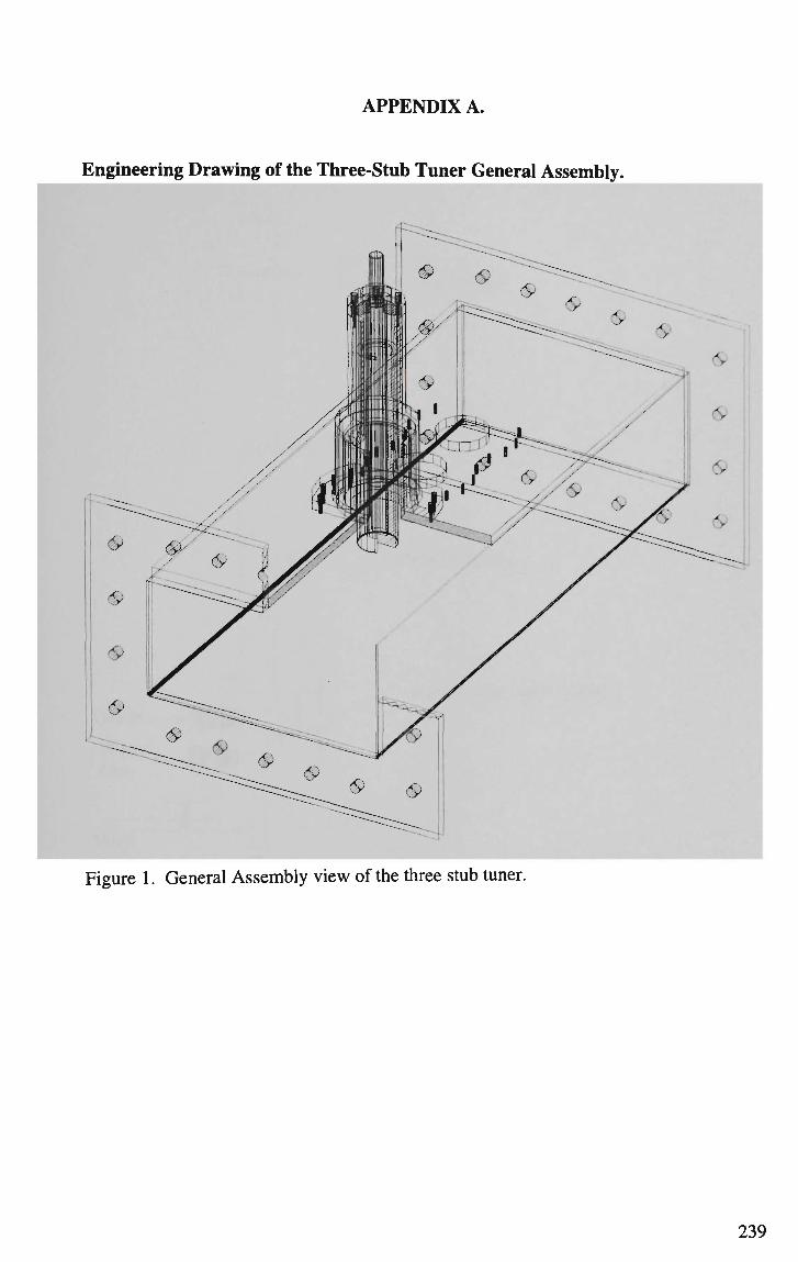
APPENDIX A.
Engineering Drawing of the Three-Stub Tuner General Assembly.
Figure 1. General Assembly view of the three stub tuner.
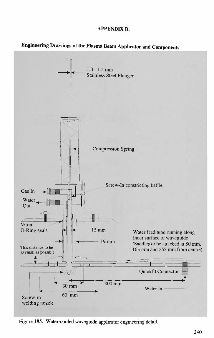
APPENDIX B.
Engineering Drawings of the Plasma Beam Applicator and Components
1.0- 1.5 mm Stainless Steel Plunger
Compression Spring
Screw-In constricting baffle
T
Viton O-Ring seals
This distance to be as small as possible
Water feed tube running along inner surface of waveguide (Saddles to be attached at 80 m m , 163 m m and 252 m m from centre)
± Quickfit Connector
30 m m 300 m m -rri
Water In
'
Screw-in welding nozzle
60 mm
Figure 185. Water-cooled waveguide applicator engineering detail.
240

Standard I Waveguide Flange
Vacuum/Pressure vessel lid constructed from 10 m m aluminium plate. Solid plate machined and welded to uprights to form a waveguide chamber.
86 mm
o
o
/4 m m tapped holes at 25 m m centres. r-110 x 106 m m cover plate attached by Allen key head bolts. -I-
V* BSP tapped hole
-G-Centreline
1.5 m m gap for electrical gasket (to be supplied at time of fabrication)
o
10 m m thick aluminium
o
Cover Plate Detail : Side View
«( 210mm •
< 190 m m •
Cover welded to upright walls to form waveguide
10 mm thick walls
o :5
o
£ VI
a CD
Machined from 6 to 3 m m thick
Machined to 3 m m thick
Machined from 6 to 3 m m thick
Plunger
-* <J
-C *d £
P. VO
•o
u c _-u £ V
s 0Q
-*(-
•a o T3
"SI y
1 _= a. £ £ Vt
o
•o
o •a
u •a ra <u £ o T5 a o
9] 00 B =1
a o S
Hole drilled from underside and tapped. N B Hole not to pierce upper surface. Diagonally opposite hole similar.
:
80 mm [180 mm
! 190 mm 210mm
10 mm holes
r )
350 m m
240 mm 400 mm
75 mm
T
Figure 186. Vacuum/Pressure vessel lid engineering detail. Plan view.
241
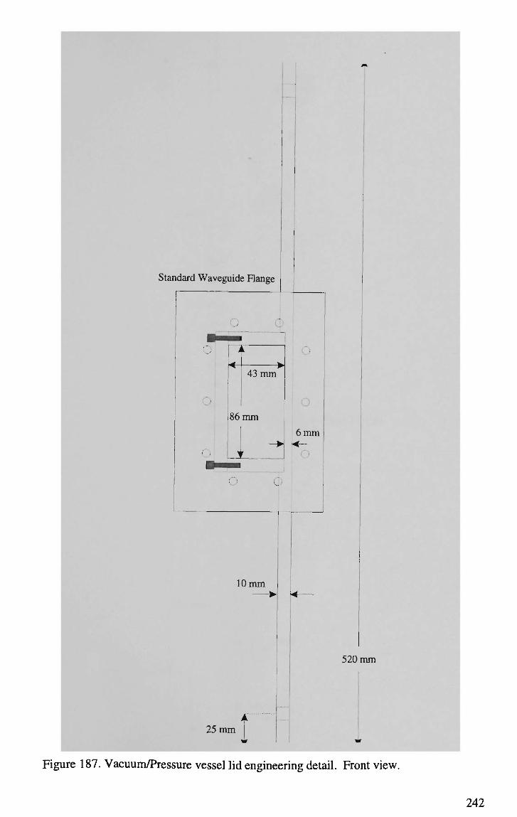
10 mm
25 mm
520 mm
Figure 187. Vacuum/Pressure vessel lid engineering detail. Front view.
242

Standard Waveguide Flange
520 m m (Diameter of Vessel Flange)
6 m m
Movable Plunger
^^^^^^^^m Figure 188. Vacuum/Pressure vessel lid engineering detail. Side view.
243

o
o
o
10 mm Holes " -XJ<
O-Ring Seal
10 m m holes 10 m m
Vacuum Flange
J
i
75 x 50 m m vacuum sealed perspex viewing port.
Side View Vacuum/Pressure vessel constructed
from 10 m m aluminium plate. Solid base plate and upper flange welded to cylindrical vessel.
32 mm
Solid Base
Annular Flange
-> <
300 mm
10mm
10mm Holes
400 mm
Figure 189. Vacuum/Pressure vessel engineering detail.
244

a •'m i'r-H"
li
'Q'
y 10 m m holes for slide rails
140 m m
Synchronous pulley belt not shown.
D
n H 0.5 m m pitch thread on height adjusters.
10 mm 20 mm
Figure 190. Welding table engineering detail. Front view.
245

2.5
\
0.5 m m Pitch
\
\
95 mm
i
' mm
sr r "
b ( j :
© 0 c
© ' z
o ( ) o LJ
120 mm
1 1
*
'
Figure 191. Welding table engineering detail. Top view.
246

15 mm
Slide Rail
45 mm
( i
40 mm
Synchronous pulleys
5 m m
Slide rail
51 mm
0.5 m m Pitch height adjustment. 2 sides linked by synchronous
pulleys and toothed belts
Vertical slide rails for height adjustment
10 m m Steel baseplate
370 mm
280 mm
Figure 192. Welding table and mounting unit engineering detail. Side view. To fit
inside vacuum/pressure vessel.

o
© Q_
A A
70 mm
140 mm
" • <~
_t
140 mm
185 mm
Figure 193. Welding table in mounting unit and positioned in vacuum/pressure vessel.
Top View.
248

300 mm
60 mm annular flange
D
10 m m spacers
J
>:
( )
5 - ^ l
r' _
C, <' )
177
'\-rO^-
( )
61 mm
10 m m holes
400 m m
10 mm
* - 80 mm
.
10 m m holes
Figure 194. Welding table in mounting unit and positioned in vacuum/pressure vessel.
Front View.
249